Conformal Regge theory

Miguel S. Costa, Vasco Goncalves, João Penedones

Centro de Física do Porto
Departamento de Física e Astronomia
Faculdade de Ciências da Universidade do Porto
Rua do Campo Alegre 687, 4169–007 Porto, Portugal

Perimeter Institute for Theoretical Physics
Waterloo, Ontario N2J 2W9, Canada

We generalize Regge theory to correlation functions in conformal field theories. This is done by exploring the analogy between Mellin amplitudes in AdS/CFT and S-matrix elements. In the process, we develop the conformal partial wave expansion in Mellin space, elucidating the analytic structure of the partial amplitudes. We apply the new formalism to the case of four point correlation functions between protected scalar operators in ${\cal N}=4$ Super Yang Mills, in cases where the Regge limit is controlled by the leading twist operators associated to the pomeron-graviton Regge trajectory. At weak coupling, we are able to predict to arbitrary high order in the ’t Hooft coupling the behaviour near $J=1$ of the OPE coefficients $C_{{\cal OO}J}$ between the external scalars and the spin $J$ leading twist operators. At strong coupling, we use recent results for the anomalous dimension of the leading twist operators to improve current knowledge of the AdS graviton Regge trajectory - in particular, determining the next and next to next leading order corrections to the intercept. Finally, by taking the flat space limit and considering the Virasoro-Shapiro S-matrix element, we compute the strong coupling limit of the OPE coefficient $C_{{\cal LL}J}$ between two Lagrangians and the leading twist operators of spin $J$.

1 Introduction

Regge theory [1, 2] is a technique to study high energy scattering. It is particularly useful when an infinite number of resonances participate in a scattering process, like it happens in QCD or in string theory. In the 60s, Regge theory was very important in organizing the phenomenology of hadrons, which suggested a stringy description. String theory was later abandoned as a theory of hadrons in favour of gauge theory (more precisely, QCD). However, we now know that conformal gauge theories are equivalent to string theory in Anti-de Sitter (AdS) space [3, 4, 5]. It is then natural to look for a generalization of Regge theory to scattering in AdS. We believe this is a good starting point to understand AdS/CFT correlation functions in the stringy regime of finite string tension (or finite ’t Hooft coupling), beyond the gravity approximation.

The goal of this paper is to generalize Regge theory of scattering amplitudes to correlation functions of conformal field theory (CFT), building on the previous work [6, 7, 8]. The main tool that we shall use is the Mellin representation of conformal correlation functions introduced in [9]. As emphasized in [9, 10, 11, 12, 13, 14, 15, 16], Mellin amplitudes are the natural analogue of scattering amplitudes for AdS/CFT. In particular, for a four-point function the Mellin amplitude depends on two variables $s$ and $t$ that are similar to the Mandelstam invariants of a scattering process in flat spacetime. Following this analogy, we confirm that Mellin amplitudes are the appropriate observable to generalize Regge theory to AdS/CFT. The main ingredients involved in our construction are summarized in table 1, which also serves as a partial outline of the paper.

We dedicate the next section to a review of Regge theory applied to string theory in flat spacetime. This will be very useful to set up the language and to guide us in the generalization for CFTs. In section 3, we review some key properties of Mellin amplitudes and introduce the conformal partial wave expansion necessary for performing the Regge theory re-summation of section 4. This gives the main result of this paper, which is summarized in the last two rows of table 1. The Mellin amplitude associated to a conformal four-point function has Regge behavior controlled by the Reggeon spin $j(\nu)$ and residue $\beta(\nu)$. Moreover, the Reggeon spin $j(\nu)$ is the inverse function of the dimension $\Delta(J)$ of the operators in the leading Regge trajectory, and the residue $\beta(\nu)$ is determined by the OPE coefficients $C_{{\cal OO}J}$ of the same operators in the OPE ${\cal OO}$ of the external operators.

In section 5, we apply the above results to the study of the Pomeron-graviton Regge trajectory in maximally supersymmetric Yang-Mills theory (SYM). One of the great values of Regge theory is that the relation between the Reggeon spin $j(\nu)$ and dimension $\Delta(J)$ of the exchanged operators does not commute with perturbation theory [17]. We shall see that the same statement applies for the relation between Regge residue $\beta(\nu)$ and OPE coefficient $C_{{\cal OO}J}$. In particular, from the two-loop calculation of the four point function of dimension two chiral primaries $\mathcal{O}$, we obtain the Regge residue at leading order in perturbation theory, and are able to compute the leading behaviour of the OPE coefficient $C_{{\cal OO}J}$ near $J=1$ to any order in the ’t Hooft coupling $\lambda=g_{\rm YM}^{2}N$. More concretely, we show that

$$C_{{\cal OO}J}^{2}=\frac{1}{N^{2}}\,\sum_{k=0}^{\infty}\lambda^{k}\left[\frac{a_{k}}{(J-1)^{k-1}}+O\left(\frac{1}{(J-1)^{k-2}}\right)\right],$$ (1)

and compute the coefficients $a_{k}$. Actually, since the Regge residue is known at next to leading order, we are also able to compute the next to leading order behaviour around $J=1$ of $C_{{\cal OO}J}$. The relation between Reggeon spin $j(\nu)$ and dimension $\Delta(J)$ also has implications to the strong coupling expansion. In particular, recent results for the anomalous dimension of the leading twist operators imply the following expansion of the AdS graviton intercept

$$j(0)=2-\frac{2}{\sqrt{\lambda}}-\frac{1}{\lambda}+\frac{1}{4\lambda^{3/2}}+\dots\,.$$ (2)

The intercept of the Pomeron-graviton Regge trajectory should interpolate between this strong coupling expansion and the BFKL weak coupling expansion. Finally, we show how the flat space limit of the correlation function in the Regge limit, together with known type IIB S-matrix elements, gives predictions for the OPE coefficients $C_{{\cal OO}J}$ involving the operators dual to the short string states in the leading Regge trajectory.

In section 6, we summarize our main findings and discuss some open avenues.

Strings in flat spacetime	CFTd or Strings in AdSd+1
Scattering amplitude	Correlation function or Mellin amplitude
$\mathcal{T}(s,t)$	$M(s,t)$
Tree-level: $g_{s}\to 0$	Planar level: $N\to\infty$
Finite string length	Finite ’t Hooft coupling
$l_{s}=\sqrt{\alpha^{\prime}}$	$\displaystyle{g^{2}\sim g_{YM}^{2}N=\frac{R^{4}}{\alpha^{\prime 2}_{\phantom{1}}}}$
Partial wave expansion	Conformal partial wave expansion
$\displaystyle{\mathcal{T}(s,t)=\sum_{J}a_{J}(t)\,\underbrace{P_{J}(\cos\theta)}_{\rm partial\ wave}}$	$\displaystyle{M(s,t)=\sum_{J_{\phantom{1}}}\int d\nu\,b_{J}(\nu^{2})\,\underbrace{M_{\nu,J}(s,t)}_{\rm partial\ wave}}$
On-shell poles	On-shell poles
$\displaystyle{a_{J}(t)\sim\frac{C^{2}(J)}{t-m^{2}(J)}}$	$\displaystyle{b_{J}(\nu^{2})\sim\frac{C^{2}(J)}{\nu^{2}+\big{(}\Delta(J)-\frac{d}{2}\big{)}^{2}_{\phantom{\frac{1}{1}}}}}$
Leading Regge trajectory	Leading twist operators
$\displaystyle{\phantom{\frac{1}{1_{1_{1}}}}m^{2}(J)=\frac{2}{\alpha^{\prime}}(J-2)\phantom{\frac{1}{1_{1_{1}}}}}$	$\Delta(J)=d-2+J+\underbrace{\gamma(J,g^{2})}_{\rm anomalous\atop dimension}$
Cubic couplings	3-pt functions or OPE coefficients
$C(J)\sim$​	$C(J)\sim$​
Regge limit: $s\to\infty$ with fixed $t$	Regge limit: $s\to\infty$ with fixed $t$
$P_{J}(\cos\theta)\approx\left(\frac{2s}{t}\right)^{J}$	$\displaystyle{M_{\nu,J}(s,t)\approx\omega_{\nu,J}(t)\,s^{J}}$
$T(s,t)\approx\beta(t)\,s^{j(t)}$	$\displaystyle{M(s,t)\approx\int_{\phantom{\frac{1}{1}}}d\nu\,\omega_{\nu,j(\nu)}(t)\,\beta(\nu)\,s^{j(\nu)}}$
Regge pole and residue	Regge pole and residue
$t-m^{2}(J)=0$ $\ \Rightarrow\$ $J=j(t)$	$\left(\Delta(J)-\frac{d}{2}\right)^{2}+\nu^{2}=0$ $\ \Rightarrow\$ $J=j(\nu)$
$\beta(t)\sim C^{2}\!\big{(}j(t)\big{)}$	$\beta(\nu)\sim C^{2}\!\big{(}j(\nu)\big{)}$

Table 1: Analogy between standard Regge theory for scattering amplitudes in flat spacetime and conformal Regge theory. The notation will be explained later, but the analogy should already be clear for readers familiarized with Regge theory (and AdS/CFT).

2 Regge theory review

This section can be safely skipped by the knowledgeable reader. We include it mostly for pedagogical purposes and to emphasize the similarity between standard Regge theory in flat space and the conformal Regge theory we introduce in section 4.

In type II superstring theory, the scattering amplitude of 4 dilatons is given by the Virasoro-Shapiro amplitude [18],

$$\mathcal{T}(s,t)=8\pi G_{N}\left(\frac{tu}{s}+\frac{su}{t}+\frac{st}{u}\right)\frac{\Gamma\big{(}1-\frac{\alpha^{\prime}s}{4}\big{)}\,\Gamma\big{(}1-\frac{\alpha^{\prime}u}{4}\big{)}\,\Gamma\big{(}1-\frac{\alpha^{\prime}t}{4}\big{)}}{\Gamma\big{(}1+\frac{\alpha^{\prime}s}{4}\big{)}\,\Gamma\big{(}1+\frac{\alpha^{\prime}u}{4}\big{)}\,\Gamma\big{(}1+\frac{\alpha^{\prime}t}{4}\big{)}}\,,$$ (3)

where $G_{N}$ is the 10-dimensional Newton constant, $\alpha^{\prime}$ is the square of the string length and

$$s=-(p_{1}+p_{3})^{2}\ ,\ \ \ \ \ \ t=-(p_{1}+p_{2})^{2}\ ,\ \ \ \ \ \ u=-(p_{1}+p_{4})^{2}\ ,$$ (4)

are the Mandelstam invariants. As the dilaton is massless the Mandelstam invariants satisfy $s+t+u=0.$ This amplitude has an infinite number of poles that correspond to the exchange of an infinite number of particles, which can be organized in Regge trajectories as shown in figure 1.

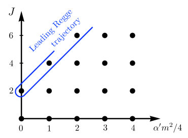
Figure 1: Chew-Frautschi plot of the spectrum of exchanged particles in the Virasoro-Shapiro amplitude.

This follows from the partial wave expansion

$$\mathcal{T}(s,t)=\sum_{J=0}^{\infty}a_{J}(t)\,P_{J}(z)\,,$$ (5)

where $P_{J}(z)$ are partial waves for 10-dimensional spacetime and

$$z=\cos\theta=1+2\,\frac{s}{t}$$ (6)

encodes the scattering angle $\theta$. In the present example only even spins contribute because the initial particles are identical scalars. To determine the spectrum of exchanged particles we use the fact that each exchanged particle of mass $m$ and spin $J$ gives rise to a pole of $a_{J}(t)$ at $t=m^{2}$. The full scattering amplitude has poles at $t=4n/\alpha^{\prime}$, for $n=0,1,2,\dots$, as can be seen in figure 1. Computing the residues of equations (3) and (5), we obtain

$$\sum_{J=0}^{\infty}P_{J}(z)\,{\rm Res}_{t=\frac{4n}{\alpha^{\prime}}}a_{J}(t)={\rm Res}_{t=\frac{4n}{\alpha^{\prime}}}\mathcal{T}(s,t)=-\frac{128\pi G_{N}}{(\alpha^{\prime}n!)^{2}}\left(\frac{nz}{2}\right)^{2+2n}+O(z^{2n})\,,$$ (8)

where the RHS is a polynomial of degree $2n+2$ in $z$, whose leading term we wrote explicitly. In fact, this equation is satisfied with a finite sum over $J$ because this is just an equality between polynomials of $z$. More precisely, it tells us that $a_{J}(t)$ has poles at $t=4n/\alpha^{\prime}$ for $n=\frac{J}{2}-1,\frac{J}{2},\frac{J}{2}+1,\dots$. The first pole in this series gives

$$a_{J}(t)\approx\frac{r(J)}{t-m^{2}(J)}\,,$$ (9)

where

$$m^{2}(J)=\frac{2}{\alpha^{\prime}}(J-2)\,,\ \ \ \ \ \ \ \ \ r(J)=-\frac{128\pi G_{N}}{\alpha^{\prime 2}\Gamma^{2}(J/2)}\left(\frac{J-2}{4}\right)^{J}\,.$$ (10)

This pole describes the leading Regge trajectory, i.e. the lightest exchanged particle for each spin $J$. The residue of the pole encodes the cubic couplings between the external particles and the exchanged particles in the leading Regge trajectory.

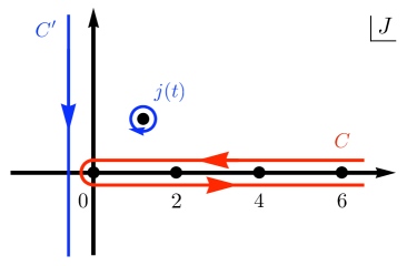
Figure 2: Integration contours in the $J$-plane involved in the Sommerfeld-Watson transform. Initially, the sum is written as an integral over the contour $C$ encircling all positive integers. Then, the contour is deformed to the contour $C^{\prime}$ plus the contribution of the Regge poles.

The goal of Regge theory is to describe the high energy limit of scattering processes. We shall think of the amplitude (3) describing elastic scattering of the initial particles 1 and 3 to the final particles 2 and 4, respectively. Thus, the Regge regime is defined by large $s$ and fixed $t$ given by (4). In this limit the amplitude (3) simplifies to

$$\mathcal{T}(s\pm i\epsilon,t)\approx\frac{32\pi G_{N}}{\alpha^{\prime}}\,e^{\mp\frac{i\pi\alpha^{\prime}t}{4}}\frac{\Gamma\big{(}-\frac{\alpha^{\prime}t}{4}\big{)}}{\Gamma\big{(}1+\frac{\alpha^{\prime}t}{4}\big{)}}\left(\frac{\alpha^{\prime}s}{4}\right)^{2+\frac{\alpha^{\prime}t}{2}}\,.$$ (11)

In this example, it was trivial to obtain the Regge limit of the scattering amplitude because we knew the exact amplitude (3). However, the achievement of Regge theory is to derive the behaviour of the amplitude in the Regge limit without knowing the full result. To understand how this works, it is instructive to stick to this example and ask the question: what is the minimal amount of information that we need to fix the amplitude in the Regge limit? The answer is the spectrum of particles in the leading Regge trajectory and their cubic couplings to the external particles. Let us review how this works.

The first step is to analytically continue the partial waves as a function of the spin $J$, and then transform the sum (5) into a contour integral in the $J$-plane,

$$\mathcal{T}(s,t)=\int_{\rm C}\frac{dJ}{2\pi i}\frac{\pi}{2\sin(\pi J)}\,a_{J}(t)\big{(}P_{J}(z)+P_{J}(-z)\big{)}\,,$$ (12)

where the contour $C$ is shown in figure 2. The symmetry property $P_{J}(-z)=(-1)^{J}P_{J}(z)$ ensures that we are only summing over even spins. The final step is to continuously deform the integration contour $C$ to the contour $C^{\prime}$ also shown in figure 2. This is possible because of the large $J$ behaviour of the partial wave

$$P_{J}(\cos\theta)\approx\frac{\cos\!\left(J\theta+\frac{7}{2}\theta+\frac{\pi}{4}\right)}{2^{J+\frac{5}{2}}\sin^{\frac{7}{2}}(\theta)}\,,$$ (13)

and because the analytically continued partial amplitude $a_{J}(t)$ does not increase exponentially in any direction in the right half of the complex $J$–plane [2]. In the contour deformation process, one picks up contributions from poles of $a_{J}(t)$ with $\text{Re}(J)>0$. These are Regge poles and are directly related to the physical poles of the scattering amplitude. In particular, the pole with largest $\text{Re}(J)$ follows from the leading Regge trajectory (9) and can be written as

$$a_{J}(t)\approx-\frac{j^{\prime}(t)\,r\big{(}j(t)\big{)}}{J-j(t)}\,,$$ (14)

where $j(t)=2+\alpha^{\prime}t/2$. The contribution of this Regge pole for the scattering amplitude reads

$$j^{\prime}(t)\,r\big{(}j(t)\big{)}\,\frac{\pi}{2\sin\!\big{(}\pi j(t)\big{)}}\left(P_{j(t)}(z)+P_{j(t)}(-z)\right)\,,$$ (15)

and therefore in the Regge limit of large $s$ we obtain

$$\mathcal{T}(s,t)\approx-\frac{32\pi^{2}G_{N}}{\alpha^{\prime}\Gamma^{2}\big{(}j(t)/2\big{)}}\left(\frac{\alpha^{\prime}}{4}\right)^{j(t)}\frac{s^{j(t)}+(-s)^{j(t)}}{\sin\!\big{(}\pi j(t)\big{)}}\,.$$ (16)

This gives exactly the Regge limit (11) of the Virasoro-Shapiro amplitude. This precise matching follows from the fact that the other Regge poles have smaller $\text{Re}(J)$ and therefore are subdominant in the Regge limit.

3 Mellin amplitudes

Mellin amplitudes were introduced by Mack in [9]. They are very convenient because they make manifest the analogy between scattering amplitudes and conformal correlation functions [10, 11, 12, 13, 14, 15, 16]. In this section, we will review the definition and discuss the main properties of Mellin amplitudes. In addition, we shall build the necessary tools for the conformal Regge theory developed in section 4.

The Mellin amplitude $M(\delta_{ij})$ associated to the connected part of the four-point function of scalar primary operators is defined by

$$A(x_{i})=\langle\mathcal{O}_{1}(x_{1})\dots\mathcal{O}_{4}(x_{4})\rangle_{\rm c}=\int[d\delta]\,M(\delta_{ij})\prod_{1\leq i<j\leq 4}\Gamma(\delta_{ij})(x_{ij}^{2})^{-\delta_{ij}}\,,$$ (17)

where the integrals run parallel to the imaginary axis. Conformal invariance constraints the integration variables to satisfy

$$\sum_{j=1}^{4}\delta_{ij}=0\,,$$ (18)

where $-\delta_{ii}\equiv\Delta_{i}$ is the dimension of the operator $\mathcal{O}_{i}$. Imposing these four constraints leaves us with two independent integration variables. The analogy with flat space scattering amplitudes becomes more explicit if we introduce fictitious momenta $p_{i}$ such that

$$\sum_{i=1}^{4}p_{i}=0\,,\ \ \ \ \ \ \ \ \ \ \ \ \delta_{ij}=p_{i}\cdot p_{j}\,.$$ (19)

Notice that due to momentum conservation the constraints (18) are automatically satisfied. It is natural to introduce the analogue of the Mandelstam invariants

$$t=-(p_{1}+p_{2})^{2}=\Delta_{1}+\Delta_{2}-2\delta_{12}\,,\ \ \ \ \ \ \ s=-(p_{1}+p_{3})^{2}-\Delta_{1}-\Delta_{4}=\Delta_{3}-\Delta_{4}-2\delta_{13}\,,$$ (20)

which we shall use as independent Mellin variables. The reduced correlator $\mathcal{A}$ is defined by

$$A(x_{i})=\frac{1}{(x_{12}^{2})^{\frac{\Delta_{1}+\Delta_{2}}{2}}(x_{34}^{2})^{\frac{\Delta_{3}+\Delta_{4}}{2}}}\left(\frac{x_{24}^{2}}{x_{14}^{2}}\right)^{\frac{\Delta_{1}-\Delta_{2}}{2}}\left(\frac{x_{14}^{2}}{x_{13}^{2}}\right)^{\frac{\Delta_{3}-\Delta_{4}}{2}}\mathcal{A}(u,v)\,,$$ (21)

such that it only depends on the conformal invariant cross ratios

$$u=\frac{x_{12}^{2}x_{34}^{2}}{x_{13}^{2}x_{24}^{2}}\ ,\ \ \ \ \ \ \ v=\frac{x_{14}^{2}x_{23}^{2}}{x_{13}^{2}x_{24}^{2}}\ .$$ (22)

Then, the reduced correlator has the following Mellin representation

$$\mathcal{A}(u,v)= \int_{-i\infty}^{i\infty}\frac{dtds}{(4\pi i)^{2}}\,M(s,t)\,u^{t/2}v^{-(s+t)/2}\,\Gamma\!\left(\frac{\Delta_{1}+\Delta_{2}-t}{2}\right)\Gamma\!\left(\frac{\Delta_{3}+\Delta_{4}-t}{2}\right)$$ (23)

$$\Gamma\!\left(\frac{\Delta_{34}-s}{2}\right)\Gamma\!\left(\frac{-\Delta_{12}-s}{2}\right)\Gamma\!\left(\frac{t+s}{2}\right)\Gamma\!\left(\frac{t+s+\Delta_{12}-\Delta_{34}}{2}\right)\,,$$

where $\Delta_{ij}=\Delta_{i}-\Delta_{j}$. The integration contours run parallel to the imaginary axis and should be placed such that the infinite series of poles produced by each $\Gamma$-function stays entirely to one side of the contour. The same requirement applies to the poles of the Mellin amplitude $M(s,t)$ itself, which are described in equation (30) below.

3.1 Operator product expansion

The structure of the OPE implies a very simple analytic structure for the Mellin amplitude if the CFT has a discrete spectrum of operator dimensions [9]. In appendix A, we explain how this works in detail.

The OPE of two scalar primary operators only contains totally symmetric and traceless tensors. It reads

$$\mathcal{O}_{1}(x)\mathcal{O}_{2}(0)=\sum_{k}\frac{C_{12k}}{(x^{2})^{\frac{1}{2}(\Delta_{1}+\Delta_{2}-\Delta)}}\left[\frac{x_{\mu_{1}}\dots x_{\mu_{J}}}{(x^{2})^{\frac{J}{2}}}\,\mathcal{O}_{k}^{\mu_{1}\dots\mu_{J}}(0)+{\rm descendants}\right],$$ (24)

where $\Delta$ and $J$ are respectively the dimension and spin of the operator $\mathcal{O}_{k}$, and all operators are normalized to have two-point function

$$\left\langle\mathcal{O}_{\mu_{1}\dots\mu_{J}}(x)\mathcal{O}_{\nu_{1}\dots\nu_{J}}(0)\right\rangle=\frac{1}{J!}\sum_{{\rm perm}\ \sigma}\frac{I_{\mu_{1}\nu_{\sigma(1)}}I_{\mu_{J}\nu_{\sigma(J)}}}{(x^{2})^{\Delta}}-{\rm traces}\,,$$ (25)

with

$$I_{\mu\nu}=\eta_{\mu\nu}-2\,\frac{x_{\mu}x_{\nu}}{x^{2}}\,.$$ (26)

This implies the following conformal block expansion of the reduced correlator

$$\mathcal{A}(u,v)=\sum_{k}C_{12k}C_{34k}\,G_{\Delta_{k},J_{k}}(u,v)\,,$$ (27)

where, in the limit $u\to 0,\ v\to 1$ with $(v-1)/\sqrt{u}$ fixed, the conformal block $G_{\Delta,J}(u,v)$ satisfies

$$G_{\Delta,J}(u,v)\approx\frac{J!}{2^{J}\left(h-1\right)_{J}}\,u^{\frac{\Delta}{2}}C_{J}^{h-1}\!\left(\frac{v-1}{2\sqrt{u}}\right).$$ (28)

In this expression $C_{J}^{h-1}$ is the Gegenbauer polynomial and we shall use throughout this paper

$$h=\frac{d}{2}\,.$$ (29)

In order to reproduce the power law behavior of $\mathcal{A}$ at small cross ratio $u$ predicted by the OPE, the Mellin amplitude must have poles in the variable $t$. More precisely,

$$M(s,t)\approx\frac{C_{12k}C_{34k}\,\mathcal{Q}_{J,m}(s)}{t-\Delta+J-2m}\,,\ \ \ \ \ \ \ \ m=0,1,2,\dots\,,$$ (30)

where, as before, $\Delta$ and $J$ are the dimension and spin of an operator $\mathcal{O}_{k}$ that appears in both OPEs $\mathcal{O}_{1}\mathcal{O}_{2}$ and $\mathcal{O}_{3}\mathcal{O}_{4}$. This shows that the $m>0$ poles correspond to conformal descendant operators with twist greater than $\Delta-J$. The residues of the poles are kinematical polynomials $\mathcal{Q}_{J,m}(s)$ of degree $J$ in the Mellin variable $s$. It is convenient to write $\mathcal{Q}_{J,m}(s)$ in terms of new polynomials $Q_{J,m}(s)$ defined by

$$\mathcal{Q}_{J,m}(s)= -\frac{2\Gamma(\Delta+J)(\Delta-1)_{J}}{4^{J}\Gamma\!\left(\frac{\Delta+J+\Delta_{12}}{2}\right)\Gamma\!\left(\frac{\Delta+J-\Delta_{12}}{2}\right)\Gamma\!\left(\frac{\Delta+J+\Delta_{34}}{2}\right)\Gamma\!\left(\frac{\Delta+J-\Delta_{34}}{2}\right)}$$ (31)

$$\frac{Q_{J,m}(s)}{m!(\Delta-h+1)_{m}\,\Gamma\!\left(\frac{\Delta_{1}+\Delta_{2}-\Delta+J}{2}-m\right)\Gamma\!\left(\frac{\Delta_{3}+\Delta_{4}-\Delta+J}{2}-m\right)}\,,$$

where we used the Pochhammer symbol

$$(a)_{m}=\frac{\Gamma(a+m)}{\Gamma(a)}=a(a+1)\dots(a+m-1)\,.$$ (32)

In appendix A we study these kinematical polynomials in detail and show, in particular, that with the above normalization

$$Q_{J,m}(s)=s^{J}+O(s^{J-1})\,.$$ (33)

In order to obtain the conformal block $G_{\Delta,J}(u,v)$ we only kept the contribution from the series of poles (30) in the integral (23). However, the integrand in (23) has more poles in the variable $t$. These poles occur at $t=\Delta_{1}+\Delta_{2}+2m$ and $t=\Delta_{3}+\Delta_{4}+2m$, which is the twist of the composite operators $\mathcal{O}_{1}\partial_{\mu_{1}}\dots\partial_{\mu_{J}}\partial^{2m}\mathcal{O}_{2}$ and $\mathcal{O}_{3}\partial_{\mu_{1}}\dots\partial_{\mu_{J}}\partial^{2m}\mathcal{O}_{4}$, in the limit where the external operators $\mathcal{O}_{i}$ interact weakly. In this paper, we shall focus on the planar part of the four-point function of single-trace operators in large $N$ gauge theories. In this case, the poles of the $\Gamma$-functions in the integrand of (23) automatically account for the contribution of double-trace operators in the OPE and the Mellin amplitude only has poles associated to single-trace contributions to the OPE.

3.2 Conformal partial waves

The first step to study Regge theory is to write down a partial wave expansion. For our purposes, the best starting point is the partial wave expansion described in [9], which is the Mellin space version of [19]. We write

$$M(s,t)=\sum_{J=0}^{\infty}\int_{-\infty}^{\infty}d\nu\,b_{J}(\nu^{2})\,M_{\nu,J}(s,t)\,,$$ (34)

with the partial waves $M_{\nu,J}(s,t)=M_{-\nu,J}(s,t)$ given by

$$M_{\nu,J}(s,t)=\omega_{\nu,J}(t)\,P_{\nu,J}(s,t)\,,$$ (35)

where

$$\omega_{\nu,J}(t)=\ \frac{\Gamma\!\left(\frac{\Delta_{1}+\Delta_{2}+J+i\nu-h}{2}\right)\Gamma\!\left(\frac{\Delta_{3}+\Delta_{4}+J+i\nu-h}{2}\right)\Gamma\!\left(\frac{\Delta_{1}+\Delta_{2}+J-i\nu-h}{2}\right)\Gamma\!\left(\frac{\Delta_{3}+\Delta_{4}+J-i\nu-h}{2}\right)}{8\pi\Gamma(i\nu)\Gamma(-i\nu)}$$

$$\frac{\Gamma\!\left(\frac{h+i\nu-J-t}{2}\right)\Gamma\!\left(\frac{h-i\nu-J-t}{2}\right)}{\Gamma\!\left(\frac{\Delta_{1}+\Delta_{2}-t}{2}\right)\Gamma\!\left(\frac{\Delta_{3}+\Delta_{4}-t}{2}\right)}\,,$$ (36)

and $P_{\nu,J}(s,t)$ is a Mack polynomial of degree $J$ in both variables $s$ and $t$. We normalized these polynomials such that they obey $P_{\nu,J}(s,t)=s^{J}+O(s^{J-1})$. The precise definition is given in appendix B.

The conformal partial wave expansion (34) is closely related to the conformal block decomposition (27). This is more easily seen if we transform (34) to position space,

$$\mathcal{A}(u,v)=\sum_{J=0}^{\infty}\int_{-\infty}^{\infty}d\nu\,b_{J}(\nu^{2})\,F_{\nu,J}(u,v)\,,$$ (37)

where $F_{\nu,J}(u,v)$ is the transform (23) of a single partial wave $M_{\nu,J}(s,t)$,

$$F_{\nu,J}(u,v)= \int_{-i\infty}^{i\infty}\frac{dtds}{(4\pi i)^{2}}\,M_{\nu,J}(s,t)\,u^{t/2}v^{-(s+t)/2}\,\Gamma\!\left(\frac{\Delta_{1}+\Delta_{2}-t}{2}\right)\Gamma\!\left(\frac{\Delta_{3}+\Delta_{4}-t}{2}\right)$$ (38)

$$\Gamma\!\left(\frac{\Delta_{34}-s}{2}\right)\Gamma\!\left(\frac{-\Delta_{12}-s}{2}\right)\Gamma\!\left(\frac{t+s}{2}\right)\Gamma\!\left(\frac{t+s+\Delta_{12}-\Delta_{34}}{2}\right).$$

In fact, $F_{\nu,J}(u,v)$ is given by the sum of two conformal blocks with dimensions $h+i\nu$ and $h-i\nu$. More precisely, one can write

$$F_{\nu,J}(u,v)=\kappa_{\nu,J}\,G_{h+i\nu,J}(u,v)+\kappa_{-\nu,J}\,G_{h-i\nu,J}(u,v)\,,$$ (39)

where the normalization constant

$$\kappa_{\nu,J}=\frac{i\nu}{2\pi K_{h+i\nu,J}}$$ (40)

can be fixed by comparing the residues of $M_{\nu,J}(s,t)$ at $t=h\pm i\nu-J+2m$ with the general expression (30), and

$$K_{\Delta,J}=\ \frac{\Gamma(\Delta+J)\,\Gamma(\Delta-h+1)\,(\Delta-1)_{J}}{4^{J-1}\Gamma\!\left(\frac{\Delta+J+\Delta_{12}}{2}\right)\Gamma\!\left(\frac{\Delta+J-\Delta_{12}}{2}\right)\Gamma\!\left(\frac{\Delta+J+\Delta_{34}}{2}\right)\Gamma\!\left(\frac{\Delta+J-\Delta_{34}}{2}\right)}$$ (41)

$$\frac{1}{\Gamma\!\left(\frac{\Delta_{1}+\Delta_{2}-\Delta+J}{2}\right)\Gamma\!\left(\frac{\Delta_{3}+\Delta_{4}-\Delta+J}{2}\right)\Gamma\!\left(\frac{\Delta_{1}+\Delta_{2}+\Delta+J-d}{2}\right)\Gamma\!\left(\frac{\Delta_{3}+\Delta_{4}+\Delta+J-d}{2}\right)}\,.$$

Notice that the two conformal blocks in (39) satisfy the same differential equation (128) because they have the same Casimir $C_{h+i\nu,J}=C_{h-i\nu,J}$. The second conformal block is usually called the shadow of the first (see for example [21] for details). Inserting (39) in (37), one can write

$$\mathcal{A}(u,v)=2\sum_{J=0}^{\infty}\int_{-\infty}^{\infty}d\nu\,b_{J}(\nu^{2})\,\kappa_{\nu,J}\,G_{h+i\nu,J}(u,v)\,,$$ (42)

which can be easily converted into the usual conformal block decomposition (27) by deforming the $\nu$-contour into the lower-half plane and picking the contribution from all poles of the integrand with negative imaginary part of $\nu$. Notice that the contribution from infinity vanishes because the conformal block $G_{h+i\nu,J}(u,v)$ decays exponentially for $\text{Im}(\nu)\to-\infty$. Thus, in order to reproduce the contribution of a single-trace operator $\mathcal{O}_{k}$ of dimension $\Delta$ and spin $J$ that appears in both OPEs $\mathcal{O}_{1}\mathcal{O}_{2}$ and $\mathcal{O}_{3}\mathcal{O}_{4}$, the partial amplitude $b_{J}(\nu^{2})$ must have poles of the form

$$b_{J}(\nu^{2})\approx C_{12k}C_{34k}\,\frac{K_{\Delta,J}}{\nu^{2}+(\Delta-h)^{2}}\,.$$ (43)

We rederive this result in appendix A.5 where we discuss the analytic structure of the partial amplitude $b_{J}(\nu^{2})$ more systematically.

4 Conformal Regge theory

We are ready to generalize Regge theory to Mellin amplitudes. To avoid cluttering of the formulae we shall restrict to the case $\Delta_{12}=\Delta_{34}=0$. It is convenient to change from the variable $s$ to the variable $z=1+\frac{2s}{t}$. We define

$$\mathcal{P}_{\nu,J}(z,t)=P_{\nu,J}\!\left(\frac{t(z-1)}{2},t\right).$$ (44)

Then, for integer spin $J$, we have the symmetry

$$\mathcal{P}_{\nu,J}(-z,t)=(-1)^{J}\mathcal{P}_{\nu,J}(z,t)\,.$$ (45)

The starting point for Regge theory is the conformal partial wave expansion (34). The construction is now analogous to that reviewed in section 2. Firstly, we analytically continue the partial amplitudes $b_{J}(\nu^{2})$ to complex values of $J$. Even and odd spins give rise to different analytic continuations $b_{J}^{+}(\nu^{2})$ and $b_{J}^{-}(\nu^{2})$, respectively. Secondly, we perform a Sommerfeld-Watson transform in (34),

$$M(s,t)=M^{+}(s,t)+M^{-}(s,t)\,,$$ (46)

with

$$M^{\pm}(s,t)=\int_{-\infty}^{\infty}d\nu\int_{\rm C}\frac{dJ}{2\pi i}\frac{\pi}{2\sin(\pi J)}\,b_{J}^{\pm}(\nu^{2})\,\omega_{\nu,J}(t)\,\big{(}\mathcal{P}_{\nu,J}(-z,t)\pm\mathcal{P}_{\nu,J}(z,t)\big{)}\,.$$ (47)

The next step in Regge theory is to deform the $J$-contour and pick up the pole with maximal real part of $J$, i.e. the leading Regge pole. Before doing this we need to consider the poles (159) of the partial amplitude $b_{J}(\nu^{2})$. We will be mostly interested in the poles associated to the leading Regge trajectory $\Delta(J)$ for $J=2,4,6,\dots$. These are the operators of lowest dimension for each even spin. This means that

$$b_{J}^{+}(\nu^{2})\approx\frac{r(J)}{\nu^{2}+\big{(}\Delta(J)-h\big{)}^{2}}\,,$$ (48)

where the residue

$$r(J)=C_{12J}C_{34J}\,K_{\Delta(J),J}\,,$$ (49)

is determined by the OPE coefficients of the operators in the leading Regge trajectory that appear in the OPEs of the external operators (see equation (43)). After analytic continuation in $J$ this pole becomes a pole in $J$, more precisely

$$b_{J}^{+}(\nu^{2})\approx-\frac{j^{\prime}(\nu)\,r(j(\nu))}{2\nu\big{(}J-j(\nu)\big{)}}\,,$$ (50)

where $j(\nu)$ is essentially the inverse function of $\Delta(J)$ defined by

$$\nu^{2}+\big{(}\Delta(j(\nu))-h\big{)}^{2}=0\,.$$ (51)

The contribution of this Regge pole is then

$$\int_{-\infty}^{\infty}d\nu\,\frac{\pi}{2\sin(\pi j(\nu))}\,\frac{j^{\prime}(\nu)\,r(j(\nu))}{2\nu}\,\omega_{\nu,j(\nu)}(t)\left(\mathcal{P}_{\nu,j(\nu)}(-z,t)+\mathcal{P}_{\nu,j(\nu)}(z,t)\right).$$ (52)

In the Regge limit ($s\to\infty$) this pole dominates and we obtain the result

$$M(s,t)\approx\int d\nu\,\beta(\nu)\,\omega_{\nu,j(\nu)}(t)\,\frac{s^{j(\nu)}+(-s)^{j(\nu)}}{\sin\!\big{(}\pi j(\nu)\big{)}}\,,$$ (53)

where

$$\beta(\nu)=\frac{\pi}{4\nu}\,j^{\prime}(\nu)\,r\big{(}j(\nu)\big{)}=\frac{\pi}{4\nu}\,j^{\prime}(\nu)\,K_{h\pm i\nu,j(\nu)}\,C_{12j(\nu)}C_{34j(\nu)}\,.$$ (54)

Equation (53) is our main result. It encodes the contribution of a Regge trajectory to the Mellin amplitude, which is fixed by conformal symmetry up to the dynamical observables $j(\nu)$ and $\beta(\nu)$. The Reggeon spin $j(\nu)$ is determined by the dimensions $\Delta(J)$ of the physical operators in the leading Regge trajectory through (51). The residue $\beta(\nu)$ is controlled by the OPE coefficients of the leading twist operators in the OPE of the external operators. This result should be valid in any CFT that has a large $N$ expansion. At leading order in $1/N$ the CFT is described by the dual AdS theory at tree-level, which implies the absence of poles in the complex $J$-plane from multi-particle states. This justifies our assumption of single Regge pole dominance.

The definition of the Regge limit of the Mellin amplitude (large $s$ and fixed $t$) corresponds to the Regge limit defined in position space in [7, 8]. This is shown in detail in appendix C. For the sake of clarity, here we just state how to relate the result (53) to the Regge limit of the correlator in position space, leaving the details to the appendix. First one needs to consider a specific Lorentzian kinematical limit where all the points are taken to null infinity. In such limit, it is convenient to introduce the variables $\sigma$ and $\rho$ that are related to the cross ratios $u$ and $v$ defined in (22) by

$$u=\sigma^{2}\,,\ \ \ \ \ \ \ v=(1-\sigma e^{\rho})(1-\sigma e^{-\rho})\approx 1-2\sigma\cosh\rho\,.$$ (55)

The Regge limit corresponds to $\sigma\to 0$ with fixed $\rho$. The position space version of equation (53) is then

$$\mathcal{A}(\sigma,\rho)\approx 2\pi i\int d\nu\,\alpha(\nu)\,\sigma^{1-j(\nu)}\Omega_{i\nu}(\rho)\,,$$ (56)

where $\Omega_{i\nu}(\rho)$ is a harmonic function on $(2h-1)$-dimensional hyperbolic space. In appendix C, we show that the residues $\alpha(\nu)$ in (56) and $\beta(\nu)$ in (53) are related by

$$\alpha(\nu)=-\frac{\pi^{h-1}2^{j(\nu)-1}e^{i\pi j(\nu)/2}}{\sin\!\left(\frac{\pi j(\nu)}{2}\right)}\,\gamma(\nu)\gamma(-\nu)\beta(\nu)\,,$$ (57)

where

$$\gamma(\nu)=\Gamma\!\left(\frac{2\Delta_{1}+j(\nu)+i\nu-h}{2}\right)\Gamma\!\left(\frac{2\Delta_{3}+j(\nu)+i\nu-h}{2}\right).$$ (58)

The form (56) was first derived in [7] applying Regge theory to the conformal partial wave expansion. Here, we have improved the result because we related the functions $\alpha(\nu)$ and $\beta(\nu)$ to the product of OPE coefficients (see equation (54)).

5 Pomeron-graviton Regge trajectory in SYM

The result (53) relates, through equation (54), the four-point function of a CFT in the Regge limit to the analytic continuation of the OPE coefficients of the operators in the leading Regge trajectory in the OPEs $\mathcal{O}_{1}\mathcal{O}_{2}$ and $\mathcal{O}_{3}\mathcal{O}_{4}$ of the external operators. In particular, (54) will allow us to make non-trivial predictions about these OPE coefficients. In this section we shall consider in detail the case of $\mathcal{N}=4$ SYM in the planar limit and its string dual, so we set $d=2h=4$.

We will consider the case of correlation functions that exchange the quantum numbers of the vacuum, so that they are dominated in the Regge limit by the exchange of the pomeron Regge trajectory. Furthermore, as external operators we shall consider BPS scalars operators, such that their dimensions are protected. At weak coupling, the operators in the pomeron-graviton Regge trajectory are a linear combination of the following twist two operators

$${\rm tr}\left(F_{\mu\nu_{1}}D_{\nu_{2}}\dots D_{\nu_{J-1}}F_{\nu_{J}}^{\ \ \mu}\right),\ \ {\rm tr}\left(\phi_{AB}D_{\nu_{1}}\dots D_{\nu_{J}}\phi^{AB}\right),\ \ {\rm tr}\left(\overline{\psi}_{A}D_{\nu_{1}}\dots D_{\nu_{J-1}}\Gamma_{\mu_{J}}\psi^{A}\right).$$ (59)

At finite ’t Hooft coupling the degeneracy is lifted and there are three different Regge trajectories. We will consider the operators in the leading Regge trajectory. In appendix E, we give the precise linear combination of the above operators that yields the spin $J$ and twist two operators of lowest dimension, to first order in perturbation theory. At strong coupling these operators are dual to massive string states, on the leading Regge trajectory of type IIB strings in AdS.

Below we shall divide the discussion in two parts, to address both weak and strong coupling expansions. We start by reviewing the consequences of conformal Regge theory to the spin-anomalous dimension function of twist two operators, as first considered in [17], and also derive some new results. We then consider the OPE coefficients.

5.1 Weak coupling

The anomalous dimension of the operators in the leading Regge trajectory is a function of the spin and of the ’t Hooft coupling. It admits the following weak coupling expansion

$$\gamma(J)=\Delta(J)-J-2=\sum_{n=1}^{\infty}g^{2n}\gamma_{n}(J)\,.$$ (60)

We use notation with coupling $g$ related to the ’t Hooft coupling $\lambda=g^{2}_{YM}N$ by

$$g^{2}=\frac{\lambda}{16\pi^{2}}\,.$$ (61)

The anomalous dimensions $\gamma_{n}$ are known up to five loops [22, 23, 24, 25] and obey the principle of maximal transcendentality [22]. The first two terms in this expansion are

$$\gamma_{1} =8S_{1}(x)\,,$$

$$\gamma_{2} =-32\big{(}S_{3}(x)+S_{-3}(x)\big{)}+64S_{-2,1}(x)-64\big{(}S_{1}(x)S_{2}(x)+S_{1}(x)S_{-2}(x)\big{)}\,,$$ (62)

where $x=J-2$ and the functions $S$ are (nested) harmonic sums, which are recursively defined by

$$S_{a_{1},a_{2},\dots,a_{n}}(x)=\sum_{y=1}^{x}\frac{({\rm sign}(a_{1}))^{y}}{y^{|a_{1}|}}\,S_{a_{2},\dots,a_{n}}(y)\,,$$ (63)

starting from the trivial seed without indices, $S(y)=1$. Some properties of these functions are given in appendix D. This weak coupling expansion of the function $\Delta(J)$ is an expansion around the free theory line $\Delta(J)=J+2$ (see figure 3).

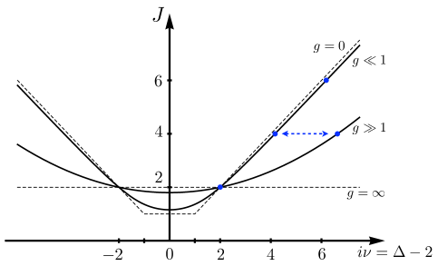
Figure 3: Leading Regge trajectory in the dimension–spin plane for various values of the ’t Hooft coupling. The physical operators have even spin $J$ and positive dimension, and are represented by blue dots along the curves. The horizontal dashed line $J=2$ corresponds to the strong coupling limit $g\to\infty$. The weak coupling limit $g\to 0$, is described by the other dashed line, with 3 branches: $J=1$, $\Delta-2=J$ and $2-\Delta=J$. The intercept $j(0)$ moves from $1$ to $2$, as the coupling $g$ goes from 0 to $\infty$.

The function $\Delta(J)$ defines the Reggeon spin $j(\nu)$. By inverting (51) we have

$$\Delta\big{(}j(\nu)\big{)}=2\pm i\nu\,.$$ (64)

However, the Reggeon spin can also be computed directly from the Regge limit of the four point correlation function [8]. At weak coupling, BFKL methods [26, 27, 28] give an expansion around the free theory value $j=1$, also shown in figure 3, associated to the exchange of two free gluons in a colour singlet. The function $j(\nu)$ is known up to next to leading order. Let us first transcribe the result presented in [22]

$$j(\nu)=1+4g^{2}\Big{(}\chi(\nu)+g^{2}\delta(\nu)\Big{)}+O(g^{6})\,,$$ (65)

with

$$\chi(\nu) =2\Psi(1)-\Psi\!\left(\frac{1+i\nu}{2}\right)-\Psi\!\left(\frac{1-i\nu}{2}\right),$$ (66)

$$\delta(\nu) =4\chi^{\prime\prime}(\nu)+6\zeta(3)-2\zeta(2)\chi(\nu)\,-2\Phi\!\left(\frac{1+i\nu}{2}\right)-2\Phi\!\left(\frac{1-i\nu}{2}\right),$$ (67)

where $\Psi(x)=\Gamma^{\prime}(x)/\Gamma(x)$ is the Euler $\Psi$-function and the function $\Phi$ is defined by

$$\Phi(x)=\frac{1}{2}\sum_{k=0}^{\infty}\frac{\Psi^{\prime}\!\left(\frac{k+2}{2}\right)-\Psi^{\prime}\!\left(\frac{k+1}{2}\right)}{k+x}\,.\ \ \ \ \ \ \ \ \ \ \ \ \ \$$ (68)

We remark that the variable $\nu$ in the spin $j(\nu)$, which appears in the BFKL amplitude as an integration variable, is exactly the same as the one in our treatment of conformal Regge theory [8]. After some manipulation, $j(\nu)$ can be written in a form which makes maximal transcendentality manifest,

$$j(\nu)=1+\sum_{n=1}^{\infty}g^{2n}\left[F_{n}\!\left(\frac{i\nu-1}{2}\right)+F_{n}\!\left(\frac{-i\nu-1}{2}\right)\right],$$ (69)

where

$$F_{1}(x) =-4S_{1}(x)\,,$$ (70)

$$F_{2}(x) =4\left(-\frac{3}{2}\,\zeta(3)+\pi^{2}\ln(2)+\frac{\pi^{2}}{3}\,S_{1}(x)+2S_{3}(x)+\pi^{2}S_{-1}(x)-4S_{-2,1}(x)\right).$$

It is important to realize that, although the functions $\Delta(J)$ and $j(\nu)$ are basically the inverse of each other, their perturbative expansions, either at weak or at strong coupling, contain different information [17]. In other words, the process of inverting the functions does not commute with perturbation theory. Let us consider first the limit $j\to 1$ and $g^{2}\to 0$, with $(j-1)/g^{2}$ fixed, of the BFKL spin (69). In this limit, only the leading order term in the expansion (69) survives, and we have

$$\frac{j(\nu)-1}{g^{2}}=-4S_{1}\!\left(\frac{i\nu-1}{2}\right)-4S_{1}\!\left(\frac{-i\nu-1}{2}\right).$$ (71)

Now, the function in the RHS of this equation has simple poles at $i\nu=\pm 1$. If we expand this equation around one of this points, say around $i\nu=1$, the fixed quantity in the LHS of this equation will be very large. This expansion has the following form

$$\frac{j(\nu)-1}{-4g^{2}}=\frac{2}{i\nu-1}-2\sum_{k=1}^{\infty}\zeta(2k+1)\,\left(\frac{i\nu-1}{2}\right)^{2k}\,,$$ (72)

where the coefficients can be read from formulae presented in appendix D. We can now invert this equation, solving for $i\nu-1=\Delta(j)-3$, to obtain the behaviour of $\Delta(J)$ around $J=1$, as a power expansion in the small quantity $g^{2}/(J-1)$. The result for the first order terms in this expansion is [17]

$$\Delta(J)-3=2\left(\frac{-4g^{2}}{J-1}\right)+0\left(\frac{-4g^{2}}{J-1}\right)^{2}+0\left(\frac{-4g^{2}}{J-1}\right)^{3}-4\zeta(3)\left(\frac{-4g^{2}}{J-1}\right)^{4}+\dots\,.$$ (73)

The remarkable thing about this expression is that, after inversion of the leading order BFKL spin, one has a prediction for the leading singularities of the anomalous dimension function (60) around $J=1$ at all orders in perturbation theory. This fact was explored in [17] and served as a guide for the computation of anomalous dimensions using integrability, most notably to check wrapping corrections that appear at four loops [29]. In the next section we shall follow a similar procedure to study the behaviour of OPE coefficients.

Let us close these introductory remarks by explaining how higher order terms in the BFKL expansion can be taken into account in the above argument. In this case one considers the expansion (69) with $(j-1)/g^{2}$ fixed, keeping all terms in the $g^{2}$ expansion, instead of only the leading term as we did in (72). Then one expands around $i\nu=1$ and inverts. The result is a prediction for the expansion of the anomalous dimension around $J=1$ at all orders in perturbation theory. In particular, the next to leading BFKL spin allows one to predict the next to leading singularity around $J=1$ at all orders in perturbation theory [17]

$$\Delta-3= \,\Big{(}0+(J-1)\Big{)}+\Big{(}2+0\left(J-1\right)\Big{)}\left(\frac{-4g^{2}}{J-1}\right)+\Big{(}0+0\left(J-1\right)\Big{)}\left(\frac{-4g^{2}}{J-1}\right)^{2}$$ (74)

$$-\Big{(}0+\zeta(3)(J-1)\Big{)}\left(\frac{-4g^{2}}{J-1}\right)^{3}-\left(4\zeta(3)+\frac{5\zeta(4)}{4}\,(J-1)\right)\left(\frac{-4g^{2}}{J-1}\right)^{4}+\dots\,.$$

Finally let us also note that we can twist around these arguments, and use the knowledge of the anomalous dimension function (60) to some fixed order in perturbation theory, to study the behaviour of the BFKL spin around $i\nu=1$. Considering the first two orders in perturbation theory for the anomalous dimension given in (62), one obtains the prediction

$$j(\nu)-1= \,\Big{(}1+0(i\nu-1)\Big{)}\left(\frac{8g^{2}}{i\nu-1}\right)+\left(\frac{1}{i\nu-1}+0\left(i\nu-1\right)\right)\left(\frac{8g^{2}}{i\nu-1}\right)^{2}$$ (75)

$$+\!\left(\frac{2}{\left(i\nu-1\right)^{2}}+\frac{0}{i\nu-1}\right)\!\left(\frac{8g^{2}}{i\nu-1}\right)^{3}\!+\left(\frac{5}{\left(i\nu-1\right)^{3}}+\frac{0}{\left(i\nu-1\right)^{2}}\right)\!\left(\frac{8g^{2}}{i\nu-1}\right)^{4}+\dots\,.$$

This result agrees with the known leading order and next to leading order BFKL spin.

5.1.1 OPE coefficients - leading order prediction

The idea is to use the knowledge of the Regge residue $\beta(\nu)$ to derive non-trivial predictions for OPE coefficients. We remind the reader that we are considering OPE coefficients with operators normalized as in (25). The product of these normalized OPE coefficients is also defined by the ratio of correlators

$$C^{2}(J)\equiv C_{11J}C_{33J}\sim\frac{\langle{\mathcal{O}}_{1}(x_{1}){\mathcal{O}}_{1}^{*}(x_{2}){\mathcal{O}}_{J}(x_{5})\rangle\,\langle{\mathcal{O}}_{J}(x_{6}){\mathcal{O}}_{3}(x_{3}){\mathcal{O}}_{3}^{*}(x_{4})\rangle}{\langle{\mathcal{O}}_{1}(x_{1}){\mathcal{O}}_{1}^{*}(x_{2})\rangle\,\langle{\mathcal{O}}_{J}(x_{5}){\mathcal{O}}_{J}(x_{6})\rangle\,\langle{\mathcal{O}}_{3}(x_{3}){\mathcal{O}}_{3}^{*}(x_{4})\rangle}\,.$$ (76)

The precise relation between the OPE coefficients and the ratio of correlators involves many kinematical factors that we give in appendix E. We omit these details to avoid dealing with all the indices in the main text. From direct computation of the the four point correlator in the Regge limit we can extract the Regge residue that appears in the correlation function (53). Then, using (54), this is related to the analytic continuation of the product of OPE coefficients $C^{2}\!\big{(}j(\nu)\big{)}$.

We start with the weak coupling side of the story. We can compute in free theory the OPE coefficient $C(J)$ of the spin $J$ operator of the leading Regge trajectory in the OPE of two protected scalar operators of the form ${\mathcal{O}}_{1}={\rm tr}(\phi_{12}\phi^{12})$, where $\phi_{12}$ is a complex scalar field of SYM. This requires lifting the degeneracy of the twist two operators and some combinatorics in doing Wick contractions. The computation is presented in appendix E, and the result is

$$C^{2}(J)=\frac{1}{N^{2}}\frac{2^{1+J}J(J-1)\Gamma^{2}(J+1)}{\left(4J^{2}-1\right)\Gamma(2J+1)}+O(g^{2})\,.$$ (77)

In particular, we can continue this result to the region around $J=1$, with an expansion of the form

$$C^{2}(J)=\frac{J-1}{N^{2}}\left(\frac{2}{3}+O(J-1)\right)+O(g^{2})\,.$$ (78)

Now let us look at the Regge residue $r(j(\nu))$ computed in perturbation theory from the four point correlation function. In [8] the Regge residue in position space $\alpha(\nu)$ was shown to be

$$\alpha(\nu)=i\,\frac{16\pi^{5}g^{4}}{N^{2}}\frac{\tanh\!\left(\frac{\pi\nu}{2}\right)}{\nu\cosh^{2}\!\left(\frac{\pi\nu}{2}\right)}+O(g^{6})\,.$$ (79)

Using (54) and (57) this translates into a residue $r(j(\nu))$ given by

$$r\big{(}j(\nu)\big{)}=-\frac{2^{8}\pi g^{2}}{N^{2}}\frac{\tanh\!\left(\frac{\pi\nu}{2}\right)}{\chi^{\prime}(\nu)(1+\nu^{2})^{2}}+O(g^{4})\,,$$ (80)

where we used the leading term in the BFKL spin as written in (65). It is clear that (80) computes the behaviour of the function $r(J)$ around $J=1$, which starts with a power of $J-1\sim g^{2}$. The same thing happens to the square of the OPE coefficients (78) computed directly in free theory. This is not a coincidence because both $r(J)$ and $C^{2}(J)$ are related by (49). Thus, for $J=j(\nu)$, we can use (49) in the form

$$r\big{(}j(\nu)\big{)}=C^{2}\!\big{(}j(\nu)\big{)}\,K_{\Delta(j({\nu})),j(\nu)}\,,$$ (81)

to compute the OPE coefficients from the Regge residue in the region $J-1\sim g^{2}$, i.e. in the double limit $g^{2}\to 0$ and $J\to 1$ with $g^{2}/(J-1)$ fixed. In particular, we will recover the above free field theory result and also make predictions to arbitrary high order in perturbation theory. The analysis is entirely analogous to that of the anomalous dimension reviewed above.

From (78) we conclude that the continuation of the OPE coefficients $C(J)$ to the region where $J-1\sim g^{2}$ admits the following general perturbative expansion

$$C^{2}(J)=(J-1)\,a\!\left(\frac{g^{2}}{J-1}\right)+O(g^{4})\,,$$ (82)

for some function $a$ that will be determined bellow. More precisely, for $J=j(\nu)$ given by (69), we have the Regge theory prediction

$$C^{2}\!\big{(}j(\nu)\big{)}=4g^{2}\chi(\nu)\,a\!\left(\frac{1}{4\chi(\nu)}\right)=\frac{r\big{(}j(\nu)\big{)}}{K_{\Delta(j(\nu)),j(\nu)}}=-\frac{2^{8}\pi g^{2}}{N^{2}}\frac{\tanh\!\left(\frac{\pi\nu}{2}\right)}{\chi^{\prime}(\nu)(1+\nu^{2})^{2}K_{\Delta(j(\nu)),j(\nu)}}\,,$$ (83)

and therefore

$$a\!\left(\frac{1}{4\chi(\nu)}\right)=-\frac{2^{6}\pi}{N^{2}}\frac{\tanh\!\left(\frac{\pi\nu}{2}\right)}{\chi(\nu)\chi^{\prime}(\nu)(1+\nu^{2})^{2}K_{2\pm i\nu,j(\nu)}}\,.$$ (84)

We want a prediction for the OPE coefficients around $J=1$, so that the function $a(x)$ can be expanded as

$$a(x)=\frac{1}{N^{2}}\left(a_{0}+a_{1}x+a_{2}x^{2}+\dots\right)\,,$$ (85)

with small $x=g^{2}/(J-1)$, therefore giving a prediction to all loops for the OPE coefficients. Thus, just like in (72) for the anomalous dimension, we need to consider equality (84) for $i\nu=\pm 1$. Notice that the function $\chi(\nu)$ has poles at $\nu=\pm i(1+2n)$, with $n=0,1,2,\dots$, so indeed we are expanding the function $a(x)$ around the origin. Moreover, we started the expansion (85) with a constant term because the RHS of (84) is regular at the origin. Doing the computation we obtained the following prediction for the first order terms in this expansion

$$a_{0}=\frac{2}{3}\,,\ \ \ \ \ a_{1}=\frac{64}{9}\,,\ \ \ \ \ a_{2}=\frac{32}{27}\left(61-3\pi^{2}\right),\ \ \ \ \ a_{3}=\frac{256}{81}\left(223-12\pi^{2}-27\zeta(3)\right),\ \dots\,.$$ (86)

The first term matches the free theory result, the other terms give a prediction for the behaviour of the OPE coefficients to any order in perturbation theory.

5.1.2 OPE coefficients - next to leading order prediction

The next to leading order correction to the function $\alpha(\nu)$ was computed in [30], with the result

$$\alpha(\nu)\!=\!i\frac{16\pi^{5}g^{4}\tanh\!\left(\frac{\pi\nu}{2}\right)}{N^{2}\nu\cosh^{2}\!\left(\frac{\pi\nu}{2}\right)}\!\left(\!1+8g^{2}\!\left(\!\frac{i\pi\chi\!\left(\nu\right)}{4}+\frac{\pi^{2}}{4}-\frac{4}{1+\nu^{2}}-\Psi^{\prime}\!\left(\frac{1-i\nu}{2}\right)-\Psi^{\prime}\!\left(\frac{1+i\nu}{2}\right)\!\right)\!\right)\,.$$ (87)

In order to reproduce this result using Regge theory, we consider the continuation of the OPE coefficients to the region close to $J=1$, keeping $g^{2}/(J-1)$ fixed, in the form

$$C^{2}(J)=\left(J-1\right)\left[a\!\left(\frac{g^{2}}{J-1}\right)+\left(J-1\right)b\!\left(\frac{g^{2}}{J-1}\right)\right]+O(g^{6})\,.$$ (88)

The first terms in the expansion of the function $a(x)$ were obtained in the previous section. Following the same procedure of matching expansions around $\nu=\pm i$, we can obtain the predictions for the function $b\left(x\right)=\sum_{k=0}^{\infty}b_{k}x^{k}$. In particular, from the result (87) for $\alpha(\nu)$ one obtains for the first term in the expansion of $b(x)$ the coefficient

$$b_{0}=\frac{2}{9}\big{(}-14+3\ln(2)\big{)}\,.$$ (89)

The prediction can be tested against the expansion of (77) computed in free theory around $J=1$. The results do not match, since (77) gives

$$b_{0}=\frac{2}{9}\big{(}-8+3\ln(2)\big{)}\,.$$ (90)

The two values differ by the rational number $4/3$, though the $log$’s do agree. Given that the free theory result is by far more trivial to derive, we speculate that perhaps some term in $\alpha(\nu)$, given by (87), is not correct. In fact, all the terms in (87) have definite transcendentality, with the exception of the term $-8/(1+\nu^{2})$. We find that if this term, which violates maximal transcendentality, is not present then there is agreement. To see this we study the dependence of $b_{0}$ on the next leading order correction to $\alpha(\nu)$. First we write,

$$\alpha(\nu)=i\,\frac{16\pi^{5}g^{4}\tanh\!\left(\frac{\pi\nu}{2}\right)}{N^{2}\nu\cosh^{2}\!\left(\frac{\pi\nu}{2}\right)}\left(1+4g^{2}\left(\sum_{k=-2}^{\infty}d_{k}(\nu-i)^{k}\right)\right)\,.$$ (91)

Matching with the expansion of $C^{2}\!\big{(}j(\nu)\big{)}$ around $\nu=\pm i$, we find that the coefficient $d_{-2}$ needs to have the value 8, in exact agreement with (87). However, in order to match the free theory result for the coefficient $b_{0}$, we must have a vanishing coefficient $d_{-1}$. This suggests that the term $-8/(1+\nu^{2})$ should indeed be absent from (87). Assuming this is the case, the conformal Regge theory prediction for the first next to leading order coefficients $b_{k}$ is,

$$b_{0}=\frac{2}{9}\big{(}-8+3\ln(2)\big{)}\,,\ \ \ \ \ b_{1}=\frac{4}{27}\big{(}-244+9\pi^{2}+48\ln(2)\big{)}\,,\ \ \ \ \$$

$$b_{2}=\frac{16}{27}\big{(}-892+122\ln(2)-2\pi^{2}\big{(}-20+3\ln(2)\big{)}+225\zeta(3)\big{)}\,,\,\dots\,.\ \ \ \$$ (92)

5.2 Strong coupling

Let us turn to the strong coupling expansion, starting again with the relation between spin and anomalous dimension of the operators in the leading Regge trajectory.

The anomalous dimensions of the leading twist operators can be computed at strong coupling from the energy of short strings in AdS, and admit an expansion of the type

$$\Delta(J)\big{(}\Delta(J)-4\big{)}=x\sum_{n=0}^{\infty}g^{1-n}H_{n}(x)\,,$$ (93)

where we conveniently defined $x=J-2$. The overall factor of $x$ guarantees that the energy momentum tensor has protected dimension. The latest results for this expansion include the one and the two loop corrections [32, 33, 34]. It is simpler to present these results in terms of the quantity $\Delta(\Delta-4)$, instead of $\Delta$, because this is the combination that appears in the Casimir of the conformal group and makes the symmetry $\Delta\to 4-\Delta$ (or $\nu\to-\nu$) explicit. The results of [32, 33, 34] then give (recall that $\sqrt{\lambda}=4\pi g$)

$$\Delta(J)\big{(}\Delta(J)-4\big{)}=x\left[2\sqrt{\lambda}+\left(-1+\frac{3x}{2}\right)-\frac{3}{8}\Big{(}-10+(8\zeta(3)-1)x+x^{2}\Big{)}\frac{1}{\sqrt{\lambda}}+\cdots\right]\,.$$ (94)

This structure suggests that $H_{n}(x)$ is a polynomial of degree $n$.

On the other hand, at strong coupling the Reggeon spin was computed using the dual string description [6, 7]

$$j(\nu)=2-\sum_{n=1}^{\infty}\frac{j_{n}(\nu^{2})}{g^{n}}=2-\frac{4+\nu^{2}}{2\sqrt{\lambda}}\left(1+\sum_{n=2}^{\infty}\frac{\widetilde{j}_{n}(\nu^{2})}{\lambda^{(n-1)/2}}\right)\,,$$ (95)

where $\widetilde{j}_{n}(\nu^{2})$, defined for $n\geq 2$, is a polynomial of degree $n-2$. The $n=1$ term in this expansion was computed in [6] and gives the linear Regge trajectory of strings in the flat space limit. The general form that constrains the degree of the polynomial $\widetilde{j}_{n}(\nu^{2})$ was derived in [7] by requiring that such limit is well defined. We will actually see that this polynomial can be further restricted.

Next we consider the limit $J\rightarrow 2$ and $\lambda\rightarrow\infty$ , with $(J-2)\sqrt{\lambda}$ fixed, of the expression for the anomalous dimension (94). Noting that $-\Delta(\Delta-4)=4+\nu^{2}$, we can equate both expansion (94) and (95) to obtain new data for the polynomials $\widetilde{j}_{n}(\nu^{2})$, with $n\geq 2$, that characterise the AdS graviton Regge trajectory. Writing

$$\widetilde{j}_{n}(\nu^{2})=\sum_{k=0}^{n-2}c_{n,k}\nu^{2k}\,,$$ (96)

we can fix the coefficients $c_{n,n-2}$ and $c_{n,n-3}$. More precisely, we obtained that

$$c_{2,0}=\frac{1}{2}\,,\ \ \ c_{3,0}=-\frac{1}{8}\,,\ \ \ c_{3,1}=\frac{3}{8}\,,\ \ \ c_{4,1}=-\frac{3}{32}\big{(}8\zeta(3)-7\big{)}\,,\ \ \ c_{5,2}=\frac{21}{64}\,,$$ (97)

and the remaining coefficients of this type vanish ($c_{n,n-2}=0$ for $n\geq 4$, $c_{n,n-3}=0$ for $n\geq 6$). In particular, we derived the next and the next to next leading order correction to the intercept

$$j(0)=2-\frac{2}{\sqrt{\lambda}}-\frac{1}{\lambda}+\frac{1}{4\lambda^{3/2}}+\dots\,.$$ (98)

From figure 4 we conclude that this strong coupling expansion works reasonably well for $g\lower 3.01385pt\hbox{$\;\stackrel{{\scriptstyle\textstyle>}}{{\sim}}\;$}0.3$. Such a strong coupling expansion has been recently used to construct phenomenological models of high energy processes in QCD that are dominated by Pomeron exchange, following the proposal of [6]. These models start from the conformal limit here studied, and then introduce a hard wall in AdS to cut off the IR scale. Data analysis of deep inelastic scattering (DIS) [36, 37, 38] and deeply virtual Compton scattering (DVCS) [39] gives an intercept in the region $j(0)=1.2-1.3$. At a first glance it may seem surprising how the fits of data in a region reasonably close to $j(0)=1$ are so successful, even better than those fits that use the weak coupling expansion (see [40] for the latest analysis on DIS). However, in SYM, figure 4 shows that indeed the strong coupling expansion seems to already work reasonably well around the region of $j(0)=1.2-1.3$.

Figure 4: Weak (in blue) and strong (in red) coupling expansions of the BFKL intercept $j(0)$. The plot suggests a smooth interpolation, like the black dashed curve, from 1 at $g=0$ to 2 at $g=\infty$.

Finally, we remark that the coefficients $c_{n,k}$ can be further restricted if we assume that $H_{l}(x)$ is a polynomial of degree $l$. This assumption leads to the conclusion that for $n\geq 4$ the coefficients satisfy

$$c_{n,k}=0\ \ \ \textrm{for}\ \ \ \left[\frac{n}{2}\right]\leq k\leq n-2\,.$$ (99)

5.2.1 OPE coefficients

Let us start with the simple case of graviton exchange in AdS between external scalar fields dual to operators of protected dimension $\Delta_{1}$ and $\Delta_{3}$. In this strict $\lambda\to\infty$ limit the spin $j(\nu)=2$ and the scattering is elastic. The Regge amplitude in position space (56) has real residue and is given by

$$\alpha(\nu)=-\frac{4\pi}{N^{2}}\,\frac{1}{4+\nu^{2}}\,\frac{\Gamma\!\left(\Delta_{1}+\frac{i\nu}{2}\right)\Gamma\!\left(\Delta_{1}-\frac{i\nu}{2}\right)\Gamma\!\left(\Delta_{3}+\frac{i\nu}{2}\right)\Gamma\!\left(\Delta_{3}-\frac{i\nu}{2}\right)}{\Gamma\!\left(\Delta_{1}\right)\Gamma\!\left(\Delta_{1}-1\right)\Gamma\!\left(\Delta_{3}\right)\Gamma\!\left(\Delta_{3}-1\right)}\,.$$ (100)

Using (57) and (54) we can relate the function $\alpha(\nu)$ to the residue $r(j(\nu))$, and therefore to the product of OPE coefficients. In the particular case of graviton exchange, we can use the first term in the expansion (95), $j(\nu)=2-(4+\nu^{2})/(2\sqrt{\lambda})+O(\lambda^{-1})$, to obtain the $\lambda\to\infty$ result

$$\alpha(\nu)=-r(2)\,\frac{16\pi^{2}}{4+\nu^{2}}\,\Gamma\!\left(\Delta_{1}+\frac{i\nu}{2}\right)\Gamma\!\left(\Delta_{1}-\frac{i\nu}{2}\right)\Gamma\!\left(\Delta_{3}+\frac{i\nu}{2}\right)\Gamma\!\left(\Delta_{3}-\frac{i\nu}{2}\right).$$ (101)

Equating the previous two equations, we can determine $r(2)$ and therefore, using (49), the product of OPE coefficients

$$C^{2}(2)=\frac{2\Delta_{1}\Delta_{3}}{45N^{2}}\,.$$ (102)

This is actually independent of $\lambda$ because the three point function with the stress-energy tensor is determined by a Ward identity [41, 42]

$$C^{2}(2)=\frac{16\Delta_{1}\Delta_{3}}{9C_{T}}\,,$$ (103)

for $\Delta_{2}=\Delta_{1}$ and $\Delta_{3}=\Delta_{4}$. Note that the central charge $C_{T}$ appears in the denominator because, as explained in (76), we are considering normalized operators. The central charge is known from gravity in AdS [43, 44]

$$C_{T}=20\,\frac{\pi R^{3}}{G_{N}^{(5)}}\,.$$ (104)

Using $G_{N}^{(5)}R^{-3}=\pi/(2N^{2})$, we obtain $C_{T}=40N^{2}$, and reproduce exactly the result (102).

The above was just a warm up exercise to make sure numerical factors are in place. We can actually compute the leading term in the strong coupling expansion of the function $C^{2}(J)$ for arbitrary $J$, therefore computing the OPE coefficients between the leading twist operators in the pomeron-graviton Regge trajectory and two external scalar operators. This can be done by considering the flat space limit of the CFT amplitude in the Regge limit, and then equating it to the flat space string theory S-matrix element with external scalar fields, also in the Regge limit, to read the function $C^{2}(J)$. As a specific example we shall consider the Virasoro-Shapiro amplitude reviewed in section 2 with external dilaton fields, which are dual to the Lagrangian operator of protected dimension $\Delta_{i}=4$.

The string theory S-matrix for four external scalars in the Regge limit can be recovered from the flat space limit introduced in [10],

$$\mathcal{T}\big{(}S,T\big{)}=\frac{1}{{\cal N}}\lim_{R\to\infty}V(S^{5})\,R\int_{-i\infty}^{i\infty}\frac{d\alpha}{2\pi i}\,\alpha^{2-\frac{\sum_{i}\Delta_{i}}{2}}e^{\alpha}\,M\!\left(\frac{R^{2}S}{2\alpha},\frac{R^{2}T}{2\alpha}\right)\,,$$ (105)

with the Mellin amplitude given by the Regge theory form (53), the volume of the 5-sphere $V(S^{5})=\pi^{3}R^{5}$ and the constant $\mathcal{N}$ given by (133). The computation now is entirely similar to the one of appendix A.2.1 for the flat space limit of a single conformal partial wave, so we will not be so detailed here (see equation (137)). The integration over $\alpha$ produces a delta function in $\nu^{2}$ with a characteristic width $L$, so in this case we have

$$\mathcal{T}\big{(}S,T\big{)}\approx \ \frac{1}{{\cal N}}\lim_{R\to\infty}V(S^{5})\,R\int_{-\infty}^{\infty}d\nu\,\beta(\nu)\,\left(\frac{R^{2}S}{2}\right)^{j(\nu)}\frac{e^{i\frac{\pi}{2}j(\nu)}}{\sin\!\left(\frac{\pi j(\nu)}{2}\right)}$$ (106)

$$\hskip 93.89418pt\frac{1}{\sqrt{\nu^{2}}}\left(\frac{-\nu^{2}}{R^{2}T}\right)^{\frac{1}{2}\sum\Delta_{i}+j(\nu)-2}\left(-R^{2}T\right)\delta_{L}\!\left(\nu^{2}+R^{2}T\right).$$

The function $\delta_{L}$ should be understood as a delta function when integrated against functions that vary in a scale $\delta\nu^{2}\gg L$. On the other hand, for functions with characteristic scale $\delta\nu^{2}\ll L$ one should take the average. For the above integral this gives

$$\mathcal{T}\big{(}S,T\big{)}\approx\ \frac{\pi R^{6}}{{\cal N}}\,\langle\beta\rangle_{T}\left(\frac{R^{2}S}{2}\right)^{J(T)}\frac{e^{i\frac{\pi}{2}J(T)}}{\sin\!\left(\frac{\pi J(T)}{2}\right)}\,,$$ (107)

where for $R\to\infty$ the graviton Regge trajectory becomes the usual linear trajectory

$$J(T)=2+\frac{\alpha^{\prime}}{2}\,T\,.$$ (108)

As explained in section A.2.1, the integration of the function $\beta(\nu)$ against the delta function $\delta_{L}$ in (106) produces the average $\langle\beta\rangle_{T}$. We shall see bellow that this is important because $\beta(\nu)$ contains a rapidly varying function of $\nu$. Note that in this case we can take the strong coupling limit of $\beta(\nu)$ given in (54), so that

$$\beta(\nu)=-\frac{\pi}{4}\,\frac{\alpha^{\prime}}{R^{2}}\,K_{\Delta\!\left(j(\nu)\right),j(\nu)}\,C^{2}\!\big{(}j(\nu)\big{)}\,.$$ (109)

Before we analyse in more detail the implications of (107), let us check that in the simplest case of $T=0$ (i.e. $J=2$) we can derive again (102). We consider the case of scattering of four dilaton fields (dual to the Lagragian operator of dimension $\Delta_{i}=4$), so that in this case $K_{\Delta\!\left(2\right),2}=5/256$ is constant. Thus there is no issue with averaging. It is then a simple exercise to equate (107) near $T=0$, to the S-matrix for graviton exchange between four dilatons, $T(S,T)=-8\pi G_{N}S^{2}/T$, checking again (102).

The S-matrix element (107) can be equated to a type IIB string theory S-matrix element in the Regge limit. Let us consider again the case of external fields given by the dilaton. Then we can equate (106) to the Virasoro Shapiro S-matrix element (3). Although the S-matrix element (107) was derived in the physical scattering region of $T<0$, we can analytically continue this expression to positive $T$. In particular this means that we can consider $J$ a positive even integer, and compute $C^{2}(J)$ at strong coupling. In this kinematical region the dimension of the exchanged leading twist operators is real. Since we work in the strong limit we have

$$\Delta(J)\approx i\nu\approx\lambda^{1/4}\sqrt{2(J-2)}\,.$$ (110)

To compute the function $C^{2}(J)$ we need to be careful with the average $\langle\beta\rangle_{T}$ of $\beta(\nu)$ in (109). Let us first look at the expansion of the function $K_{\Delta(J),J}$ at large $\Delta$ and for external operators of dimension four,

$$K_{\Delta(J),J}\approx\frac{2^{9+2J+2\Delta(J)}\big{(}\Delta(J)\big{)}^{-10-2J}}{\pi^{3}}\sin^{2}\!\left(\frac{\pi\Delta(J)}{2}\right).$$ (111)

Thus, when integrating $\beta(\nu)$ given by (109) against the function $\delta_{L}$, this $sin^{2}$ piece is rapidly varying and averages to $1/2$. In addition, we shall assume that the remaining dependence on $\beta(\nu)$ in $\nu$ is power law, so its integration with the function $\delta_{L}$ works like with a delta function. Thus, after some straightforward algebra, we can write the flat space limit of this CFT amplitude in the following form

$$\mathcal{T}(S,T)\approx \ \frac{1}{{\cal N}}\,\frac{N^{2}G_{N}}{2\pi\alpha^{\prime}}\,\left\langle K_{\Delta\!\left(j(\nu)\right),j(\nu)}\,C^{2}\!\big{(}j(\nu)\big{)}\right\rangle_{T}$$ (112)

$$\left(\frac{R^{4}}{\alpha^{\prime 2}}\right)^{\frac{\alpha^{\prime}T}{4}}e^{\mp i\pi\frac{\alpha^{\prime}T}{4}}\,\Gamma\!\left(1+\frac{\alpha^{\prime}T}{4}\right)\Gamma\!\left(-\frac{\alpha^{\prime}T}{4}\right)\left(\frac{\alpha^{\prime}S}{2}\right)^{J(T)},$$

where, for the external operators under consideration, ${\cal N}=1/(1152\pi^{2})$. Finally equating to the Virasoro-Shapiro amplitude in the Regge limit (11), we obtain the following strong coupling prediction for the OPE coefficient involving two Lagrangians and a spin $J$ operator in the leading Regge trajectory,

$$C_{{\cal L}{\cal L}J}\approx\frac{\pi^{\frac{3}{2}}}{3N}\,\frac{(J-2)^{\frac{5+J}{2}}}{2^{1+J}\Gamma\!\left(\frac{J}{2}\right)}\,\lambda^{\frac{7}{4}}\,2^{-\lambda^{1/4}\sqrt{2(J-2)}}\,.$$ (113)

The exponential dependence on the coupling comes precisely from the dimension of the spin $J$ operator. This is expected since the AdS computation of the three point function should be dominated by the saddle point of the dual heavy short string. It would be very interesting to derive this result using the methods of [45, 46, 47].

6 Conclusion

The first lesson of this work is that the analogy between Mellin amplitudes and scattering amplitudes can be very fruitful to guide the exploration of AdS/CFT at finite or strong coupling. In this paper, we studied the regime of high energy scattering and successfully developed conformal Regge theory following the analogy summarized in table 1. Then, in section 5, we applied the formalism to SYM and obtained non-trivial predictions for the dimension $\Delta(J)$ of the spin $J$ leading twist operator and its OPE coefficient $C(J)$ in the OPE of two protected scalar operators, both at weak and strong coupling.

We conclude by discussing some questions for the future. In the context of SYM, there are two obvious directions to pursue. Firstly, we can study other Regge trajectories with different quantum numbers. In particular, it would be interesting to study the Regge limit of the four-point function

$$\left\langle{\rm Tr}\!\left(XZ\right)\!(x_{1})\,{\rm Tr}\!\left(\overline{X}Z\right)\!(x_{2})\,{\rm Tr}\!\left(Y\overline{Z}\right)\!(x_{3})\,{\rm Tr}\!\left(\overline{Y}\overline{Z}\right)\!(x_{4})\right\rangle,$$ (114)

where $X$, $Y$ and $Z$ are complex scalar fields of SYM. This would give information about the (simpler) three-point functions

$$\left\langle{\rm Tr}\!\left(Y\overline{Z}\right)\!(x_{1})\,{\rm Tr}\!\left(\overline{Y}\overline{Z}\right)\!(x_{2})\,{\rm Tr}\!\left(ZD^{J}Z\right)\!(x_{3})\right\rangle,$$ (115)

that describe the coupling of the external operators to the leading Regge trajectory in this charged sector. These were recently computed to three-loop order in [48], and were also studied in [49]. Secondly, we can apply the conformal Regge theory formalism to higher orders in perturbation theory, exploring the abundance of available data for four-point functions in SYM [50, 51]. Notice that from the four-point function at order $g^{2l}$, it is possible to extract the pomeron spin at order $g^{2l-4}$. This means that from the six loops ($l=6$) integral representation of the four-point function given in [51], one can, in principle, obtain the BFKL pomeron spin at order $g^{8}$ or next to next to next to leading order!

More generally, one can pose the question: Are all planar n-point functions of SYM determined by the planar two and three point functions of single-trace operators? It is clear that single-trace data is not sufficient information from the OPE point of view. However, it is sufficient information to fix all poles and residues of the Mellin amplitudes. Therefore, as speculated in [10], it should be possible to fix all Mellin amplitudes if we understand their asymptotic behaviour. The main result (53) of this paper, can be thought as a first step in this direction. Indeed, we were able to determine the Regge limit of the four-point function solely in terms of dimensions and OPE coefficients of single-trace operators. We believe there is a refined OPE formalism for planar (conformal) gauge theories, that distinguishes single-trace from multi-trace operators, waiting to be discovered.

In this paper, we discussed an analogy between standard Regge theory for scattering amplitudes and conformal Regge theory. However, in some theories, one can interpolate from one to the other. Consider a conformal gauge theory deformed by a relevant operator that leads to confinement in the infrared. As an example, one can think of weakly coupled SYM with a large mass $M$ for the matter fields, such that there is a large hierarchy between $M$ and the lightest glueball mass $M_{g}$. Glueball scattering in this theory will be described by standard Regge theory for $M_{g}^{2},T\ll S\ll M^{2}$, and by conformal Regge theory in the extreme high energy regime $S\gg T\gg M^{2}\gg M_{g}^{2}$. It would be interesting to understand this transition in detail. The basic mechanism is that the continuous variable $\nu$ of conformal Regge theory, becomes a discrete variable labelling several Regge trajectories in the confining theory. In other words, one conformal Regge trajectory breaks up into many standard Regge trajectories [52, 53, 6].

Appendix A Mellin amplitudes in more detail

In this appendix, we collect several results that complement the description of Mellin amplitudes of section 3.

A.1 Mellin Poles

As stated in the main text, the structure of the conformal OPE implies a very simple analytic structure for the Mellin amplitude if the CFT has a discrete spectrum of operator dimensions [9]. Here we shall explain how this works in more detail. Some of the results of this section were already discussed in [9, 10, 20, 13], however we shall take the risk of repetition with the hope of making more transparent key features that are needed in Regge theory.

The OPE implies the conformal block expansion (27) of the reduced correlator, which we rewrite here for convenience

$$\mathcal{A}(u,v)=\sum_{k}C_{12k}C_{34k}\,G_{\Delta_{k},J_{k}}(u,v)\,.$$ (116)

As explained in [42], the conformal blocks have a series expansion of the form

$$G_{\Delta,J}(u,v)=u^{\frac{\Delta-J}{2}}\sum_{m=0}^{\infty}u^{m}g_{m}(v)\,,$$ (117)

where the first term reads

$$g_{0}(v)=\left(\frac{v-1}{2}\right)^{J}\ _{2}F_{1}\!\left(\frac{\Delta+J-\Delta_{12}}{2},\frac{\Delta+J+\Delta_{34}}{2},\Delta+J,1-v\right)\,.$$ (118)

In order to reproduce the power law behavior of $\mathcal{A}$ at small cross ratio $u$ predicted by the OPE, the Mellin amplitude must have poles in the variable $t$. More precisely,

$$M(s,t)\approx\frac{C_{12k}C_{34k}\,\mathcal{Q}_{J,m}(s)}{t-\Delta+J-2m}\,,\ \ \ \ \ \ \ \ m=0,1,2,\dots\,,$$ (119)

where, as before, $\Delta$ and $J$ are the dimension and spin of an operator $\mathcal{O}_{k}$ that appears in both OPEs $\mathcal{O}_{1}\times\mathcal{O}_{2}$ and $\mathcal{O}_{3}\times\mathcal{O}_{4}$. The integer $m$ that labels the poles in (119) corresponds precisely to the label $m$ in (117). This shows that the $m>0$ poles correspond to conformal descendant operators with twist greater than $\Delta-J$. The residues of the poles are the kinematical polynomials $\mathcal{Q}_{J,m}(s)$ given in (31). To determine these polynomials we require that the contribution of the series of poles (119) reproduces the conformal block $G_{\Delta,J}(u,v)$. Picking the poles (119) in the integral (23) one obtains a series of the form (117) with

$$g_{m}(v)=\frac{2\Gamma(\Delta+J)(\Delta-1)_{J}}{4^{J}m!(\Delta-h+1)_{m}\,\Gamma\!\left(\frac{\Delta+J+\Delta_{12}}{2}\right)\Gamma\!\left(\frac{\Delta+J-\Delta_{12}}{2}\right)\Gamma\!\left(\frac{\Delta+J+\Delta_{34}}{2}\right)\Gamma\!\left(\frac{\Delta+J-\Delta_{34}}{2}\right)}$$ (120)

$$\int_{-i\infty}^{i\infty}\frac{ds}{8\pi i}\,v^{-(s+\tau)/2}Q_{J,m}(s)\,\Gamma\!\left(\frac{\Delta_{34}-s}{2}\right)\Gamma\!\left(\frac{-\Delta_{12}-s}{2}\right)\Gamma\!\left(\frac{\tau+s}{2}\right)\Gamma\!\left(\frac{\tau+s+\Delta_{12}-\Delta_{34}}{2}\right),$$

where $\tau=\Delta-J+2m$. This explains the position of the poles (119) of the Mellin amplitude.

Let us consider first the $m=0$ case. Expanding (120) in powers of $(1-v)$ and using the explicit expression of $g_{0}(v)$ in (118), we obtain the following set of equations

$$\frac{(-2)^{J}\Gamma\!\left(\frac{\Delta-J-\Delta_{12}}{2}+n\right)\Gamma\!\left(\frac{\Delta-J+\Delta_{34}}{2}+n\right)\Gamma\!\left(\frac{\Delta+J+\Delta_{12}}{2}\right)\Gamma\!\left(\frac{\Delta+J-\Delta_{34}}{2}\right)n!}{\Gamma(\Delta+n)(\Delta-1)_{J}(n-J)!}=$$ (121)

$$= \int_{-i\infty}^{i\infty}\frac{ds}{4\pi i}\,Q_{J,0}(s)\,\Gamma\!\left(\frac{\Delta_{34}-s}{2}\right)\Gamma\!\left(\frac{-\Delta_{12}-s}{2}\right)\Gamma\!\left(\frac{\tau+s}{2}+n\right)\Gamma\!\left(\frac{\tau+s+\Delta_{12}-\Delta_{34}}{2}\right).$$

For $n<J$ the LHS vanishes and this equation can be written as follows

$$0= \int_{-i\infty}^{i\infty}\frac{ds}{4\pi i}\,Q_{J,0}(s)\left(\frac{\tau+s}{2}\right)_{n}$$ (122)

$$\Gamma\!\left(\frac{\Delta_{34}-s}{2}\right)\Gamma\!\left(\frac{-\Delta_{12}-s}{2}\right)\Gamma\!\left(\frac{\tau+s}{2}\right)\Gamma\!\left(\frac{\tau+s+\Delta_{12}-\Delta_{34}}{2}\right).$$

Taking linear combinations of this equation with $n<J$, we conclude that it defines an inner product under which $Q_{J,0}(s)$ is orthogonal to all polynomials of $s$ with degree less than $J$. In other words, the polynomials $Q_{J,0}(s)$ must satisfy

$$\delta_{J,J^{\prime}}\propto \int_{-i\infty}^{i\infty}\frac{ds}{4\pi i}\,Q_{J,0}(s)\,Q_{J^{\prime},0}(s)$$ (123)

$$\Gamma\!\left(\frac{\Delta_{34}-s}{2}\right)\Gamma\!\left(\frac{-\Delta_{12}-s}{2}\right)\Gamma\!\left(\frac{\tau+s}{2}\right)\Gamma\!\left(\frac{\tau+s+\Delta_{12}-\Delta_{34}}{2}\right).$$

This fixes the polynomials $Q_{J,0}(s)$ uniquely, up to normalization. The normalization can be fixed by imposing (121) for any $n\geq J$.

The orthogonality of the polynomials $Q_{J,0}(s)$ suggests that they are the solutions of a Sturm-Liouville problem. Indeed, the difference operator $\mathcal{D}_{s}$, defined by

$$\mathcal{D}_{s}Q(s)=(s+\tau+\Delta_{12}-\Delta_{34})\Big{[}(s+\tau)Q(s+2)-2sQ(s)\Big{]}+(s+\Delta_{12})(s-\Delta_{34})Q(s-2)\,,$$ (124)

is self-adjoint with respect to the inner product above. Therefore, eigenfunctions of $\mathcal{D}_{s}$ with different eigenvalues are automatically orthogonal. By construction, the action of $\mathcal{D}_{s}$ on a polynomial of $s$ of degree $J$ produces another polynomial of $s$ of degree $J$. Thus, we can look for polynomial eigenfunctions of $\mathcal{D}_{s}$,

$$\mathcal{D}_{s}\,Q_{J,0}(s)=\lambda_{J}\,Q_{J,0}(s)\,.$$ (125)

The eigenvalue $\lambda_{J}$ is fixed by comparing the coefficient of the highest degree term $s^{J}$, with the result

$$\lambda_{J}=4J^{2}+4J(\tau-1)+(\tau+\Delta_{12})(\tau-\Delta_{34})\,.$$ (126)

Finally, the solution can be written in terms of hypergeometric functions

$$Q_{J,0}(s)=\frac{2^{J}\left(\frac{\Delta_{12}+\tau}{2}\right)_{J}\left(\frac{\Delta_{34}+\tau}{2}\right)_{J}}{\left(\tau+J-1\right)_{J}}\,_{3}F_{2}\!\left(-J,J+\tau-1,\frac{\Delta_{34}-s}{2};\frac{\tau+\Delta_{12}}{2},\frac{\tau+\Delta_{34}}{2};1\right).$$ (127)

Consider now the case $m>0$. The best way to determine the functions $g_{m}(v)$ is to use the differential equation that the conformal block satisfies,

$$\mathcal{D}\,G_{\Delta,J}(u,v)=\frac{1}{2}\,C_{\Delta,J}\,G_{\Delta,J}(u,v)\,,$$ (128)

where

$$\mathcal{D}= \,(1-u-v)\,\frac{\partial}{\partial v}\left(v\frac{\partial}{\partial v}+\frac{\Delta_{34}-\Delta_{12}}{2}\right)+u\frac{\partial}{\partial u}\left(2u\frac{\partial}{\partial u}-d\right)$$ (129)

$$-(1+u-v)\left(u\frac{\partial}{\partial u}+v\frac{\partial}{\partial v}-\frac{\Delta_{12}}{2}\right)\left(u\frac{\partial}{\partial u}+v\frac{\partial}{\partial v}+\frac{\Delta_{34}}{2}\right),$$

and $C_{\Delta,J}=\Delta(\Delta-d)+J(J+d-2)$ is the conformal quadratic Casimir. This equation was derived in [55] and it has a simple meaning: the conformal block is an eigenfunction of the conformal Casimir operator $(J^{AB}_{1}+J^{AB}_{2})^{2}$ that acts on points 1 and 2. When applied to the power series (117) this partial differential equation turns into the following (differential) recursion relation for the functions $g_{m}(v)$,

$$4v(v-1)^{2}g_{m}^{\prime\prime}(v)-2(v-1)g_{m}^{\prime}(v)\big{(}2v(-\Delta+J-2m-1)+\Delta_{12}(v-1)-\Delta_{34}(v-1)+2\big{)}$$

$$+g_{m}(v)\Big{(}4m(-2h+mv+m)+J^{2}(v-1)-2J\big{(}\Delta+2m(v+1)+\Delta v-2\big{)}$$

$$+(v-1)\big{(}\Delta_{12}\left(-\Delta-\Delta_{34}+J-2m\right)+\Delta_{34}(\Delta-J+2m)\big{)}+4\Delta m(v+1)+\Delta^{2}(v-1)\Big{)}$$

$$=\ 4v(v+1)g_{m-1}^{\prime\prime}(v)+2g_{m-1}^{\prime}(v)\big{(}2v(\Delta-J+2m-1)-\Delta_{12}(v+1)+\Delta_{34}(v+1)+2\big{)}$$

$$+g_{m-1}(v)\left(-\Delta+\Delta_{12}+J-2m+2\right)\left(-\Delta-\Delta_{34}+J-2m+2\right)\,.$$ (130)

This is an ugly equation which the reader should not read in detail. Nevertheless, it is not hard to check that $g_{0}(v)$ given by (118) solves the $m=0$ equation. Most importantly, if we replace $g_{m}(v)$ given by (120) in equation (130), we obtain a set of recursion relations for the polynomials $Q_{J,m}(s)$,

$$\left(\mathcal{D}_{s}-\lambda_{J}\right)Q_{J,m}(s)=4m(h-\Delta-m)\big{(}2Q_{J,m}(s)-Q_{J,m-1}(s+2)-Q_{J,m-1}(s)\big{)}\,,$$ (131)

where $\mathcal{D}_{s}$ and $\lambda_{J}$ are respectively given by (124) and (126) with $\tau=\Delta-J+2m$. This equation, plus the boundary condition $Q_{J,0}(s)=s^{J}+O(s^{J-1})$ which follows from (127), determine the polynomials $Q_{J,m}(s)$ for all $m\geq 0$. In particular, it is clear that the leading behaviour is given by (33) for all $m$. This follows from the fact that the LHS of (131) is automatically a polynomial of degree $(J-1)$, if we assume that $Q_{J,m}(s)$ is a polynomial of degree $J$. Imposing the same condition to the RHS implies that $Q_{J,m}(s)$ and $Q_{J,m-1}(s)$ have the same leading behaviour.

A.2 Flat space limit

In AdS/CFT, the radius $R$ of AdS in units of the string length $l_{s}$ is a free parameter related to the ’t Hooft coupling of the gauge theory. Therefore, it should be possible to recover bulk flat space physics by taking the limit $R/l_{s}\to\infty$ and keeping energies fixed in string units. Given the similarity between Mellin amplitudes and scattering amplitudes it is not surprising that there is a simple formula that relates them. Such a formula was proposed in [10] and rederived in [13] using localized wavepackets. It reads

$$\mathcal{T}(p_{i})=\frac{1}{\mathcal{N}}\lim_{R\to\infty}R^{2h-3}\int_{-i\infty}^{i\infty}\frac{d\alpha}{2\pi i}\,\alpha^{h-\frac{1}{2}\sum\Delta_{i}}\,e^{\alpha}\,M\!\left(\delta_{ij}=\frac{R^{2}}{2\alpha}\,p_{i}\cdot p_{j}\right),$$ (132)

where the integration contour runs to the right of all poles of the integrand and

$$\mathcal{N}=\frac{1}{8\pi^{h}}\prod_{i=1}^{4}\frac{1}{\sqrt{\Gamma(\Delta_{i})\Gamma(\Delta_{i}-h+1)}}\,.$$ (133)

In formula (132), $M$ is the Mellin amplitude of a CFT four-point function of single-trace operators $\mathcal{O}_{i}$ and $\mathcal{T}$ is the scattering amplitude of the dual bulk fields $\phi_{i}$.

A relevant example for the present paper is the tree-level exchange of a spin $J$ and mass $m$ particle. In flat space, this gives rise to

$$\mathcal{T}=g^{2}\,T^{J-1}f\!\left(\frac{S}{T},\frac{m^{2}}{T}\right),$$ (134)

where $S$ and $T$ are the Mandelstam invariants, $g$ is a dimensionful coupling constant and $f$ is a dimensionless function. Then, formula (132) tells us that the Mellin amplitude associated to the tree-level exchange of a spin $J$ and dimension $\Delta$ field in AdS has the following asymptotic behaviour

$$M(s,t)=g^{2}R^{5-2h-2J}\,t^{J-1}\widetilde{f}\!\left(\frac{s}{t},\frac{\Delta^{2}}{t}\right)+O(t^{J-2})\,,$$ (135)

with

$$f\left(x,y\right)=\frac{2^{1-J}}{\mathcal{N}}\int_{-i\infty}^{i\infty}\frac{d\alpha}{2\pi i}\,\alpha^{h-\frac{1}{2}\sum\Delta_{i}-J+1}\,e^{\alpha}\,\widetilde{f}(x,2y\alpha)\,.$$ (136)

A.2.1 Flat space limit of conformal partial wave expansion

Next we study the flat space limit (132) of the conformal partial wave expansion (34),

$$\mathcal{T}(p_{i})=\frac{1}{\mathcal{N}}\sum_{J=0}^{\infty}\lim_{R\to\infty}R^{2h-3}\int_{-\infty}^{\infty}d\nu\,b_{J}(\nu^{2})\int_{-i\infty}^{i\infty}\frac{d\alpha}{2\pi i}\,\alpha^{h-\frac{1}{2}\sum\Delta_{i}}\,e^{\alpha}\,M_{\nu,J}\!\left(\frac{R^{2}S}{2\alpha},\frac{R^{2}T}{2\alpha}\right).$$ (137)

In order to compute the large $R$ limit of the integral it would be useful to know what is the integration region in $\nu$ and $\alpha$ that dominates the integral for large $R$. We shall start by assuming that the integral is dominated by $\nu^{2}\gg 1$ and later check that this is indeed the case. Using the Stirling expansion of the $\Gamma$-function we find

$$\omega_{\nu,J}(t)\approx\frac{1}{\sqrt{\nu^{2}}}\left(\frac{-\nu^{2}}{2t}\right)^{\frac{1}{2}\sum\Delta_{i}+J-h}\exp\left\{\nu\arctan\!\left(\frac{\nu}{t}\right)-\frac{t}{2}\log\!\left(1+\frac{\nu^{2}}{t^{2}}\right)\right\},$$ (138)

where we are assuming $-t=-\frac{R^{2}T}{2\alpha}\gg|\nu|\gg 1$. In appendix B we consider the limit $|t|\sim|s|\gg|\nu|\gg 1$ of the Mack polynomials, and obtain

$$P_{\nu,J}(s,t)\approx\left(\frac{t}{2}\right)^{J}P_{J}(z)\,,$$ (139)

where $P_{J}(z)$ are the partial waves in $(2h+1)$-dimensional flat spacetime and $z=1+\frac{2s}{t}$. Using these two approximations (137) becomes

$$\mathcal{T}(p_{i})=\ \frac{1}{\mathcal{N}}\sum_{J=0}^{\infty}P_{J}(z)\lim_{R\to\infty}R^{2h-3}\left(\frac{R^{2}T}{4}\right)^{J}\int_{-\infty}^{\infty}d\nu\,b_{J}(\nu^{2})\,\frac{1}{\sqrt{\nu^{2}}}\left(\frac{-\nu^{2}}{R^{2}T}\right)^{\frac{1}{2}\sum\Delta_{i}+J-h}$$

$$\int_{-i\infty}^{i\infty}\frac{d\alpha}{2\pi i}\exp\left\{\alpha+\nu\arctan\!\left(\frac{2\alpha\nu}{R^{2}T}\right)-\frac{R^{2}T}{4\alpha}\log\!\left(1+\left(\frac{2\alpha\nu}{R^{2}T}\right)^{2}\right)\right\},$$ (140)

where now $z=\cos\theta=1+\frac{2S}{T}$ encodes the flat space scattering angle. Let us discuss the integral (140). If we expand the exponent at large $R$, we obtain

$$\int_{-i\infty}^{i\infty}\frac{d\alpha}{2\pi i}\exp\left\{\alpha\left(1+\frac{\nu^{2}}{R^{2}T}\right)-\frac{2\alpha^{3}\nu^{4}}{3R^{6}T^{3}}+O\!\left(\frac{1}{R^{10}}\right)\right\}.$$ (141)

Keeping only the first term in this exponential, the integral over $\alpha$ gives rise to a delta-function $\delta\!\left(1+\frac{\nu^{2}}{R^{2}T}\right)$. This justifies the initial assumption of large $\nu^{2}$. However, one must be careful because the delta-function follows from taking the integrand to be a plane wave in $\alpha$, for all values of $\alpha$. This is clearly wrong since for $\alpha\sim R^{2}T/\nu^{4/3}$ the second term in the exponent becomes of order 1. In fact, we can perform the integral over $\alpha$ keeping only the first two terms in the exponent, obtaining

$$\frac{R^{2}T}{(2\nu^{4})^{1/3}}\,{\rm Ai}\!\left(\frac{\nu^{2}+R^{2}T}{(2\nu^{4})^{1/3}}\right),$$ (142)

where Ai is the Airy function. This expression means that the integral over $\nu$ is dominated by the region $\nu^{2}\sim-R^{2}T\pm\nu^{4/3}\sim-R^{2}T\pm(-R^{2}T)^{2/3}$. At large $R$, both the mean value of $\nu^{2}$ and the width of the region are large, but the mean is much larger than the width. Including higher order corrections in (141), leads to corrections to the function of $\nu^{2}$ (142) in smaller scales than $(-R^{2}T)^{2/3}$ but still much larger than 1. Therefore, we conclude that the flat space limit of the conformal partial wave expansion gives the standard partial wave expansion,

$$\mathcal{T}=\sum_{J=0}^{\infty}P_{J}(z)\,a_{J}(T)\,,$$ (143)

with the flat space partial amplitudes given by the limit

$$a_{J}(T)=\frac{1}{\mathcal{N}}\lim_{R\to\infty}R^{2h-3}\left(\frac{R^{2}T}{4}\right)^{J}\,\langle b_{J}\rangle_{T}\,,$$ (144)

where

$$\langle b_{J}\rangle_{T}=\int dx\,\delta_{L}(x)\,b_{J}\big{(}-R^{2}T+x\big{)}$$ (145)

is an averaging of the conformal partial amplitudes $b_{J}(\nu^{2})$ around $\nu^{2}=-R^{2}T$ with a function $\delta_{L}(x)$ which is a regulated delta-function with characteristic width $L=(-R^{2}T)^{2/3}$.

The flat space limit of conformal blocks in Mellin space was first studied in [13]. The main novelty of our result is the averaging (145). As we saw in the specific example studied in section 5.2.1, the practical effect of this averaging is simply to smooth out rapid oscillations of $b_{J}(\nu^{2})$, which should not be present in the flat space partial waves $a_{J}(T)$.

A.3 Example: Witten diagrams

Consider the Witten diagram in figure 5a associated with the exchange of a dimension $\Delta$ and spin $J$ field in AdS. The OPE expansion of the corresponding four-point function in the (12)(34) channel contains double-trace operators and the single-trace operator dual to the exchanged field in AdS [56, 57, 58]. The OPE expansion in the other channels only contains double-trace operators. This means that the only poles of the associated Mellin amplitude are given by equation (30). In addition, we know from the flat space limit analysis of the previous section that this Mellin amplitude is polynomially bounded at large values of $s$ and $t$. Thus, we conclude that it can be written as a sum of poles plus an analytic piece, which is a polynomial $\mathcal{R}_{J-1}$ of degree $J-1$ in both variables $s$ and $t$,

$$M(s,t)=C_{12k}C_{34k}\sum_{m=0}^{\infty}\frac{\mathcal{Q}_{J,m}(s)}{t-\Delta+J-2m}+\mathcal{R}_{J-1}(s,t)\,.$$ (146)

Let us see if this results agrees with the expectations from the bulk point of view. To compute the Witten diagram in figure 5a we need to know what is the precise form of the cubic vertices. However, there is a unique cubic vertex between 2 scalar fields and a spin $J$ field if we are allowed to use the equations of motion.

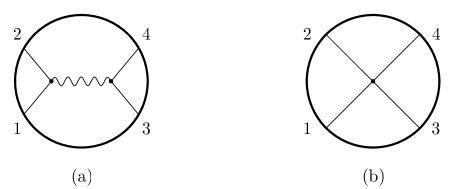
Figure 5: Witten diagrams of (a) exchange of a dimension $\Delta$ and spin $J$ field in AdS and (b) contact interaction.

This is directly related to the fact that there is a unique conformal three-point function between 2 scalar operators and a spin $J$ operator (see [59] for a more complete discussion of this correspondence). On the other hand, the internal line of the diagram 5a is not on-shell and, therefore, the equations of motion will not give zero, but will transform the internal propagator into a delta-function. This means that different cubic vertices will produce correlation functions that differ by contact diagrams like the one in figure 5b. In fact, it is not hard to convince ourselves that this contact diagrams can have at most $2J-2$ derivatives. As explained in [10], this implies that the associated Mellin amplitude is a polynomial of degree $J-1$. Thus, the result (146) is exactly what one expects from the bulk point of view. The Mellin amplitude contains a polynomial $\mathcal{R}_{J-1}$ that encodes the precise choice of cubic couplings, and a sum of poles completely fixed by the OPE coefficients of the exchanged operator $\mathcal{O}_{k}$ in the OPEs of $\mathcal{O}_{1}\mathcal{O}_{2}$ and $\mathcal{O}_{3}\mathcal{O}_{4}$. Similar arguments were recently given in [16].

A.3.1 Regge limit

Something nice happens in the Regge limit of large $s$ and fixed $t$. Firstly, the non-universal part $\mathcal{R}_{J-1}$ of the Mellin amplitude (146) drops out. Secondly, the polynomials $Q_{J,m}(s)$, introduced in (31), can be replaced by their asymptotic behavior (33). This gives

$$M(s,t)\approx C_{12k}C_{34k}\,f(t)\,s^{J}\,,$$ (147)

with

$$f(t)= -\frac{2\Gamma(\Delta+J)(\Delta-1)_{J}}{4^{J}\Gamma\!\left(\frac{\Delta+J+\Delta_{12}}{2}\right)\Gamma\!\left(\frac{\Delta+J-\Delta_{12}}{2}\right)\Gamma\!\left(\frac{\Delta+J+\Delta_{34}}{2}\right)\Gamma\!\left(\frac{\Delta+J-\Delta_{34}}{2}\right)}$$ (148)

$$\sum_{m=0}^{\infty}\frac{1}{m!(\Delta-h+1)_{m}\,\Gamma\!\left(\frac{\Delta_{1}+\Delta_{2}-\Delta+J-2m}{2}\right)\Gamma\!\left(\frac{\Delta_{3}+\Delta_{4}-\Delta+J-2m}{2}\right)(t-\Delta+J-2m)}\,.$$

Fortunately, this sum has a nice integral representation [10]

$$f(t)=K_{\Delta,J}\int d\nu\,\frac{\omega_{\nu,J}(t)}{(\Delta-h)^{2}+\nu^{2}}\,\,,$$ (149)

where $\omega_{\nu,J}(t)$ is given in (36) and the normalization constant $K_{\Delta,J}$ is given in (41).

In the Regge limit, it is striking how similar is the behavior of the Mellin amplitude (147) for an exchange of a spin $J$ field in AdS, and the corresponding flat space scattering amplitude. Both grow as $s^{J}$ (or $S^{J}$) times a function of $t$ (or $T$). In the integral representation (149) the infinite sequence of poles in $t$ is generated by a single pole in $\nu^{2}$. Indeed, this pole is the best analogue to the unique pole in $T$ of the flat space scattering amplitude.

A.4 Double trace operators

Let us briefly remark how double trace operators, that also appear in the conformal block decomposition (27), are generated in the conformal partial wave expansion (34). The double traces are generated by poles of $\kappa_{\nu,J}$ at

$$i\nu =\Delta_{1}+\Delta_{2}+J+2m-h\,, m =0,1,2,\dots\,,$$ (150)

$$i\nu =\Delta_{3}+\Delta_{4}+J+2m-h\,, m =0,1,2,\dots\,.$$ (151)

The product of the OPE coefficients of a double-trace operator $\widetilde{\mathcal{O}}_{k}\sim\mathcal{O}_{1}\partial_{\mu_{1}}\dots\partial_{\mu_{J}}\partial^{2m}\mathcal{O}_{2}$, of dimension $\widetilde{\Delta}_{k}=\Delta_{1}+\Delta_{2}+\widetilde{J}+2m$ and spin $\widetilde{J}$, in the OPE $\mathcal{O}_{1}\mathcal{O}_{2}$ and $\mathcal{O}_{3}\mathcal{O}_{4}$, is given by

$$\widetilde{C}_{12k}\widetilde{C}_{34k}=\ \frac{4^{J}\Gamma\!\left(\frac{\widetilde{J}+\Delta_{3}+\Delta_{4}-\widetilde{\Delta}_{k}}{2}\right)\Gamma\!\left(\frac{-2h+\widetilde{J}+\Delta_{3}+\Delta_{4}+\widetilde{\Delta}_{k}}{2}\right)\Gamma\!\left(\frac{\widetilde{J}-\Delta_{34}+\widetilde{\Delta}_{k}}{2}\right)\Gamma\!\left(\frac{\widetilde{J}+\Delta_{34}+\widetilde{\Delta}_{k}}{2}\right)}{m!\Gamma\!\left(\widetilde{J}+\widetilde{\Delta}_{k}\right)\left(h-\widetilde{\Delta}_{k}+1\right)_{m}\left(\widetilde{\Delta}_{k}-1\right)_{\widetilde{J}}}$$

$$\Gamma\!\left(\widetilde{J}+m+\Delta_{1}\right)\Gamma\!\left(\widetilde{J}+m+\Delta_{2}\right)b_{\widetilde{J}}\!\left(-\left(\widetilde{\Delta}_{k}-h\right)^{2}\right)\,.$$ (152)

To illustrate the use of this formula consider the correlator associated to the Witten diagram of figure 5a describing the exchange of a spin $J$ and dimension $\Delta$ field in AdS. In the previous section, we concluded that the corresponding Mellin amplitude was a polynomial of degree $J$ in the variable $s$. This implies that the conformal partial wave expansion (34) obeys $b_{J^{\prime}}(\nu^{2})=0$ for $J^{\prime}>J$. Thus, the Regge limit of (34) is simply given by

$$M(s,t)\approx s^{J}\,\int_{-\infty}^{\infty}d\nu\,b_{J}(\nu^{2})\,\omega_{\nu,J}(t)\,.$$ (153)

Comparing with the results (147) and (149) for the Regge limit of the Witten diagram of figure 5a, we conclude that

$$b_{J}(\nu^{2})=C_{12k}C_{34k}\,\frac{K_{\Delta,J}}{\nu^{2}+(\Delta-h)^{2}}\,,$$ (154)

where $C_{12k}C_{34k}$ is the product of the OPE coefficients of the operator dual to the field exchanged in AdS. Notice that in this case, the partial amplitude $b_{J}(\nu^{2})$ is exactly given by the sum of the two simple poles predicted in (43). The partial amplitudes $b_{J^{\prime}}(\nu^{2})$ for $J^{\prime}<J$ are more complicated and are not determined by the Regge limit. It is then trivial to use $b_{J}(\nu^{2})$ given by (154) in (152), to immediatelly obtain the OPE coefficients of the double trace operators of maximal spin $\widetilde{J}=J$ produced by the Witten diagram of figure 5a.

A.5 Analytic structure of partial amplitudes

The pole structure of the partial amplitudes $b_{J}(\nu)$ is directly related to the spectrum of single-trace operators that appear in both OPEs $\mathcal{O}_{1}\mathcal{O}_{2}$ and $\mathcal{O}_{3}\mathcal{O}_{4}$. The mechanism is the following: the poles (30) of the Mellin amplitude arise from the integral over $\nu$ in (34) when the integration contour is pinched between two poles of the integrand as depicted in figure 6. The partial wave $M_{\nu,J}(s,t)$ introduced in (35) has the following poles in the variable $\nu$,

$$\pm i\nu =\Delta_{1}+\Delta_{2}+J-h+2m\,, \ \ \ m =0,1,2,\dots\,,$$ (155)

$$\pm i\nu =\Delta_{3}+\Delta_{4}+J-h+2m\,, \ \ \ m =0,1,2,\dots\,,$$ (156)

$$\pm i\nu =h-J-t+2m\,, m =0,1,2,\dots\,,$$ (157)

$$\pm i\nu =h-1+J-q\,, \ \ \ q =1,2,\dots,J\,,$$ (158)

where the first three sets of poles come from the function $\omega_{\nu,J}(t)$ defined in (36), and the last line are poles of the polynomial $P_{\nu,J}(s,t)$ defined in appendix B.

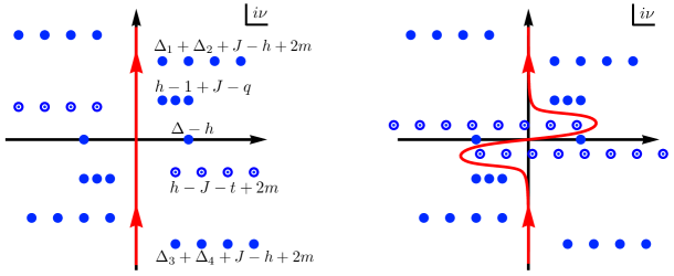
Figure 6: Integration contour in the $i\nu$ complex plane used in the conformal partial wave expansion (34). The blue dots represent poles of the integrand given by (155-158) and (159). In order to make the figure readable, we have complexified several parameters to separate the poles better. The poles (157) that depend on $t$ are marked with a small dot enclosed by a circle. As $t$ varies these poles move and can collide with other poles pinching the integration contour, as shown on the right panel. This is the mechanism that generates the poles (30) of the Mellin amplitude.

In order to obtain poles in the variable $t$ from the integral over $\nu$ in (34), a pole from (157) must collide with another $\nu$ pole. In fact, in order to reproduce the poles (30) with the correct residue one needs the partial amplitudes $b_{J}(\nu^{2})$ to have the following pair of $\nu$ poles

$$b_{J}(\nu^{2})\approx C_{12k}C_{34k}\,\frac{K_{\Delta,J}}{\nu^{2}+(\Delta-h)^{2}}\,,$$ (159)

where the normalization constant $K_{\Delta,J}$ is given in (41). When $t$ approaches $\Delta-J+2m$ with $m=0,1,2,\dots$, two poles from (157) collide with the two poles (159), pinching the $\nu$-contour in (34) and producing a divergent integral (see figure 6). To check that the resulting poles in $t$ of the Mellin amplitude have the correct residues it is sufficient to keep the contribution from the poles (159) to the integral (34) using the Cauchy theorem,

$$M(s,\Delta-J+2m+\delta t) \approx C_{12k}C_{34k}\,K_{\Delta,J}\,\frac{2\pi}{\Delta-h}\,M_{i(\Delta-h),J}(s,\Delta-J+2m+\delta t)$$

$$\approx C_{12k}C_{34k}\,\frac{\mathcal{Q}_{J,m}(s)}{\delta t}\,,$$ (160)

in perfect agreement with (30). To obtain this result it was crucial to use the property (176) of the Mack polynomials. We conclude that for every single-trace operator that appears in both OPEs $\mathcal{O}_{1}\mathcal{O}_{2}$ and $\mathcal{O}_{3}\mathcal{O}_{4}$, the partial amplitudes $b_{J}(\nu^{2})$ will have a pair of poles of the form (159).

Unfortunately, the story is slightly more complicated and cumbersome because $b_{J}(\nu^{2})$ has other (spurious) poles that do not correspond to any operators appearing in the OPEs. To explain this let us systematically analyze all possible contour pinchings in (34) that can give rise to poles in $t$. Suppose a pole from (157) collides with a pole from (155). This would give rise to a pole at $t=\Delta_{1}+\Delta_{2}+2m$ for $m=0,1,2,\dots$. However, this pole is cancelled by a zero of $\omega_{\nu,J}(t)$ produced by the last $\Gamma$-functions in the denominator of (36). A similar statement applies to collision with the poles (156). Another possibility is the collision of 2 poles of the form (157) themselves. This happens when $J+t-h$ is a non-negative integer, which means that the colliding poles are located at integer values of $i\nu$. Thus, this collision also does not generate poles in $t$ because the function $\omega_{\nu,J}(t)$ has zeros at integer values of $i\nu$. The final possibility is for the poles (157) to collide with the poles (158) of the Mack polynomials. Let us focus on the contribution of one the poles (158) for a fixed value of $J$ and $q$. This gives rise to a series of poles in $t$ of the form (30) with dimension $\Delta^{\prime}$, spin $J^{\prime}$ and OPE coefficients $C_{12k}^{\prime}C_{34k}^{\prime}$ given by

$$\Delta^{\prime} =2h-1+J\,,$$ (161)

$$J^{\prime} =J-q\,,$$ (162)

$$C_{12k}^{\prime}C_{34k}^{\prime} =\frac{\mathcal{Z}_{J,q}}{K_{\Delta^{\prime},J^{\prime}}}\,b_{J}\big{(}-(h-1+J-q)^{2}\big{)}\,,$$ (163)

where $K_{\Delta,J}$ is given in (41) and

$$\mathcal{Z}_{J,q}=\frac{J!}{(J-q)!q!}\frac{2(-2)^{q}\left(\frac{\Delta_{1}+\Delta_{2}+1-2h-q}{2}\right)_{q}\left(\frac{\Delta_{3}+\Delta_{4}+1-2h-q}{2}\right)_{q}\left(\frac{\Delta_{12}+1-q}{2}\right)_{q}\left(\frac{\Delta_{34}+1-q}{2}\right)_{q}}{\Gamma(q)(h+J-q)_{q-1}}\,.$$ (164)

In order to derive this result we used the property (179) of the Mack polynomials given in appendix B. This result looks strange because it says that the OPE will generically contain primary operators of dimension $\Delta^{\prime}$ (which is an integer or half-integer). This can not be the case. In fact, what happens is that the partial amplitudes $b_{J^{\prime}}(\nu^{2})$, with $J^{\prime}=J-q$ have other poles that cancel this effect. This requirement fixes the new residues to be

$$b_{J-q}(\nu^{2})\approx-\frac{\mathcal{Z}_{J,q}\,b_{J}\big{(}-(h-1+J-q)^{2}\big{)}}{\nu^{2}+(h-1+J)^{2}}\,,\ \ \ \ \ \ \ \ \ \ q=1,2,3,\dots\,J.$$ (165)

These poles were termed spurious poles in [7]. We believe that the relation (165) is the translation to our language of the identity (2.59b) of [19], which discusses a similar conformal partial wave expansion (although in position space).

Appendix B Mack polynomials

With our normalizations, the polynomials introduced in [9] can be written as

$$P_{\nu,J}(s,t)= \,\sum_{r=0}^{[J/2]}a_{J,r}\frac{2^{J+2r}\left(\frac{h+i\nu-J-t}{2}\right)_{r}\left(\frac{h-i\nu-J-t}{2}\right)_{r}(J-2r)!}{\left(h+i\nu-1\right)_{J}\left(h-i\nu-1\right)_{J}}$$ (166)

$$\sum_{\sum k_{ij}=J-2r}(-1)^{k_{13}+k_{24}}\prod_{(ij)}\frac{(\delta_{ij})_{k_{ij}}}{k_{ij}!}\prod_{n=1}^{4}\left(\alpha_{n}\right)_{J-r-\sum_{j}k_{jn}}\,.$$

In this expression the labels $(ij)$ run over the 4 possibilities (13), (14), (23) and (24). The variables $\delta_{ij}$ are as before,

$$\delta_{13}=\frac{\Delta_{34}-s}{2}\,,\ \ \ \delta_{24}=-\frac{\Delta_{12}+s}{2}\,,\ \ \ \delta_{23}=\frac{t+s}{2}\,,\ \ \ \delta_{14}=\frac{t+s+\Delta_{12}-\Delta_{34}}{2}\,.$$ (167)

The variables $\alpha_{n}$ are given by

$$\alpha_{1}=1-\frac{h+i\nu+J+\Delta_{12}}{2}\,,\ \ \ \ \ \ \alpha_{2}=1-\frac{h+i\nu+J-\Delta_{12}}{2}\,,$$ (168)

$$\alpha_{3}=1-\frac{h-i\nu+J+\Delta_{34}}{2}\,,\ \ \ \ \ \ \alpha_{4}=1-\frac{h-i\nu+J-\Delta_{34}}{2}\,.$$

The coefficients $a_{J,r}$ define the flat $(2h+1)$-dimensional spacetime partial waves

$$P_{J}(z)=\sum_{r=0}^{[J/2]}a_{J,r}\,z^{J-2r}\,,\ \ \ \ \ \ a_{J,r}=(-1)^{r}\,\frac{J!(h+J-1)_{-r}}{2^{2r}r!(J-2r)!}\,.$$ (169)

It is clear from the definition (166) that $P_{\nu,J}(s,t)$ is indeed a polynomial of degree $J$ in both variables $t$ and $s$. Let us check that the leading term is $s^{J}$, as stated in the main text. This must come from the $r=0$ term in the sum (166),

$$P_{\nu,J}(s,t)\approx\frac{s^{J}J!}{\left(h+i\nu-1\right)_{J}\left(h-i\nu-1\right)_{J}}\,\sum_{\sum k_{ij}=J}\,\prod_{(ij)}\frac{1}{k_{ij}!}\,\prod_{n=1}^{4}\left(\alpha_{n}\right)_{J-\sum_{j}k_{jn}}\,,$$ (170)

where we have kept only the leading term in $s$ in the Pochhammer symbols $(\delta_{ij})_{k_{ij}}$. To perform the last sum we change to the variables $q_{1}=J-k_{13}-k_{14}$ and $q_{3}=J-k_{13}-k_{23}$. Then the sum over $k_{ij}$ in (170) can be written as

$$\sum_{q_{1}=0}^{J}\,\sum_{q_{3}=0}^{J}\,\sum_{k_{13}=0}^{J-q_{1}}\,\frac{\left(\alpha_{1}\right)_{q_{1}}\left(\alpha_{2}\right)_{J-q_{1}}\left(\alpha_{3}\right)_{q_{3}}\left(\alpha_{4}\right)_{J-q_{3}}}{k_{13}!\,(J-q_{1}-k_{13})!\,(J-q_{3}-k_{13})!\,(q_{1}+q_{3}-J+k_{13})!}$$ (171)

$$= \ J!\,\sum_{q_{1}=0}^{J}\,\frac{\left(\alpha_{1}\right)_{q_{1}}\left(\alpha_{2}\right)_{J-q_{1}}}{q_{1}!\,(J-q_{1})!}\,\sum_{q_{3}=0}^{J}\,\frac{\left(\alpha_{3}\right)_{q_{3}}\left(\alpha_{4}\right)_{J-q_{3}}}{(q_{3})!\,(J-q_{3})!}=\frac{\left(\alpha_{1}+\alpha_{2}\right)_{J}\left(\alpha_{3}+\alpha_{4}\right)_{J}}{J!}\,.$$

Using the definitions (168) it follows that $P_{\nu,J}(s,t)\approx s^{J}$.

There are several symmetry properties that follow from the formula (166) by relabelling the summation variables,

$$k_{13}\leftrightarrow k_{24}\ \ \ \Rightarrow\ \ P_{-\nu,J}\big{(}s,t,\Delta_{12},\Delta_{34}\big{)}=P_{\nu,J}\big{(}s,t,-\Delta_{34},-\Delta_{12}\big{)}$$ (172)

$$k_{14}\leftrightarrow k_{23}\ \ \ \Rightarrow\ \ P_{-\nu,J}\big{(}s,t,\Delta_{12},\Delta_{34}\big{)}=P_{\nu,J}\big{(}s+\Delta_{12}-\Delta_{34},t,\Delta_{34},\Delta_{12}\big{)}$$ (173)

and

$$\left\{{k_{13}\leftrightarrow k_{14}\atop k_{23}\leftrightarrow k_{24}}\right.\ \ \ \Rightarrow\ \ P_{\nu,J}\big{(}s,t,\Delta_{12},-\Delta_{34}\big{)}=(-1)^{J}P_{\nu,J}\big{(}-s-t-\Delta_{12},t,\Delta_{12},\Delta_{34}\big{)}$$ (174)

$$\left\{{k_{13}\leftrightarrow k_{23}\atop k_{14}\leftrightarrow k_{24}}\right.\ \ \ \Rightarrow\ \ P_{\nu,J}\big{(}s,t,-\Delta_{12},\Delta_{34}\big{)}=(-1)^{J}P_{\nu,J}\big{(}-s-t+\Delta_{34},t,\Delta_{12},\Delta_{34}\big{)}$$ (175)

In fact, there is a more basic invariance, $P_{-\nu,J}(s,t)=P_{\nu,J}(s,t)$, which is not obvious from the definition (166). These symmetries were first discussed in [20].

Another important property is that the Mack polynomials, at specific values of $t$, reduce to the polynomials $Q_{J,m}(s)$ that control the OPE as explained in section 3.1,

$$P_{i(\Delta-h),J}(s,\Delta-J+2m)=Q_{J,m}(s)\,.$$ (176)

Consider now the limit $t\sim s\gg 1$ and $\nu^{2}\gg 1$. In equation (166), it is sufficient to replace the Pochhammer symbols $(x)_{n}$ of a large quantity $x$ by the leading term $x^{n}$. This gives

$$P_{\nu,J}(s,t)\approx \sum_{r=0}^{[J/2]}a_{J,r}\,4^{r-J}\left(t^{2}+\nu^{2}\right)^{r}(J-2r)!\sum_{\sum k_{ij}=J-2r}\frac{s^{k_{13}+k_{24}}(t+s)^{k_{14}+k_{23}}}{k_{13}!\,k_{24}!\,k_{14}!\,k_{23}!}$$

$$= \sum_{r=0}^{[J/2]}a_{J,r}\,2^{-J}\left(t^{2}+\nu^{2}\right)^{r}\sum_{q=0}^{J-2r}\frac{(J-2r)!}{q!\,(J-2r-q)!}\,s^{q}(t+s)^{J-2r-q}$$ (177)

$$= \left(\frac{t^{2}+\nu^{2}}{4}\right)^{\frac{J}{2}}\,\sum_{r=0}^{[J/2]}a_{J,r}\,\left(\frac{t+2s}{\sqrt{t^{2}+\nu^{2}}}\right)^{J-2r}=\left(\frac{t^{2}+\nu^{2}}{4}\right)^{\frac{J}{2}}P_{J}\!\left(\frac{t+2s}{\sqrt{t^{2}+\nu^{2}}}\right).$$

If we further assume $|t|\gg|\nu|$, we obtain

$$P_{\nu,J}(s,t)\approx\left(\frac{t}{2}\right)^{J}P_{J}(z)\,,$$ (178)

where $z=1+2s/t$. This limit was first studied in [13].

The definition (166) also makes it clear that $P_{\nu,J}(s,t)$ is polynomial in the parameters $\Delta_{12}$ and $\Delta_{34}$. On the other hand, we see that $P_{\nu,J}(s,t)$ has poles at $\nu=\pm i(h+J-q-1)$ for $q=1,2,\dots,J$. We checked that the residues of these poles are described by the formula,

$$P_{\nu,J}(s,t)\approx\frac{2^{q}J!\left(\frac{\Delta_{12}-q+1}{2}\right)_{q}\left(\frac{\Delta_{34}-q+1}{2}\right)_{q}\left(\frac{2h-t-q+1}{2}\right)_{q}}{\left(h+J-q-1\pm i\nu\right)q!\,(J-q)!\,\Gamma(q)\,(h-1+J-q)_{q}}\,P_{i(h+J-1),J-q}(s,t)\,,$$ (179)

for all $J\leq 8$. We believe that this is an identity, but were unable to prove it.

Appendix C Regge limit in position space

This appendix has two goals. The first one is to show that our definition of the Regge limit of the Mellin amplitude (large $s$ and fixed $t$) corresponds to the Regge limit defined in position space in [7, 8]. This limit can be defined by $x_{1}^{+}\to\lambda x_{1}^{+}$, $x_{2}^{+}\to\lambda x_{2}^{+}$, $x_{3}^{-}\to\lambda x_{3}^{-}$, $x_{4}^{-}\to\lambda x_{4}^{-}$ and $\lambda\to\infty$, keeping the causal relations $x_{14}^{2},x_{23}^{2}<0$ and all the other $x_{ij}^{2}>0$. This is depicted in figure 7. We remark that by Fourier transforming to momentum space the position of the operators $x_{i}$, and defining the corresponding Mandelstam invariants, the Regge limit is just the usual Regge limit of large $s$ and fixed $t$. The second goal of this appendix is to derive an expression for the position space correlator in the Regge limit corresponding to our main equation (53).

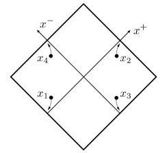
Figure 7: Conformal compactification of the light cone plane. In the Regge limit the positions of the operators $x_{i}$ go to null infinity.

Let us then start by the definition of the Mellin representation for the time ordered Lorentzian correlation function [9]

$$A(x_{i})=\int[d\delta]\,M(\delta_{ij})\prod_{i<j}\Gamma(\delta_{ij})\big{(}x_{ij}^{2}+i\epsilon\big{)}^{-\delta_{ij}}\,.$$ (180)

Given the chosen causal relations for the Regge limit, we should rotate

$$v^{-(s+t)/2}\to v^{-(s+t)/2}e^{-i\pi(s+t)}$$ (181)

in the integral (23). With this phase, the convergence of the integral is not obvious when $s=ix$, $x\to+\infty$. To study this question, we approximate the second line of (23) using

$$\Gamma\!\left(a+i\,\frac{x}{2}\right)\Gamma\!\left(b-i\,\frac{x}{2}\right)\approx 2\pi\,e^{i\frac{\pi}{2}(a-b)}\left(\frac{x}{2}\right)^{a+b-1}e^{-\frac{\pi}{2}x}\,,\ \ \ \ \ \ \ x\to+\infty\,.$$ (182)

This gives

$$\mathcal{A}(u,v)\approx\int_{-i\infty}^{i\infty}\frac{dt}{4i}\,u^{t/2}v^{-t/2}\,\Gamma\!\left(\frac{2\Delta_{1}-t}{2}\right)\Gamma\!\left(\frac{2\Delta_{3}-t}{2}\right)e^{-i\pi\frac{t}{2}}\int^{\infty}\!\!dx\,M(ix,t)\left(\frac{x}{2}\right)^{t-2}v^{-\frac{i}{2}x}\,,$$ (183)

where we have restricted to the case $\Delta_{12}=\Delta_{34}=0$. Following [7, 8], we introduce the variables $\sigma$ and $\rho$ via

$$u=\sigma^{2}\,,\ \ \ \ \ \ \ v=(1-\sigma e^{\rho})(1-\sigma e^{-\rho})\approx 1-2\sigma\cosh\rho\,,$$ (184)

such that the Regge limit corresponds to $\sigma\to 0$ with fixed $\rho$. In this limit,

$$\mathcal{A}\approx\int_{-i\infty}^{i\infty}\frac{dt}{4i}\,\sigma^{t}\,\Gamma\!\left(\frac{2\Delta_{1}-t}{2}\right)\Gamma\!\left(\frac{2\Delta_{3}-t}{2}\right)e^{-i\pi\frac{t}{2}}\int^{\infty}\!\!dx\,M(ix,t)\left(\frac{x}{2}\right)^{t-2}e^{ix\sigma\cosh\rho}\,,$$ (185)

which shows that the small $\sigma$ behavior of $\mathcal{A}$ is controlled by the large $s$ behavior of the Mellin amplitude. We can now use our main result (53) to write

$$M(ix,t)\approx\int d\nu\,\beta(\nu)\,\frac{x^{j(\nu)}}{\sin\!\left(\frac{\pi j(\nu)}{2}\right)}\,\omega_{\nu,j(\nu)}(t)\,,$$ (186)

where we have chosen the appropriate phase for $s=ix$, $x\to+\infty$. After performing the integral over $x$, we find

$$\mathcal{A}\approx -\pi i\int d\nu\,\beta(\nu)\,\frac{e^{i\pi j(\nu)/2}}{\sin\!\left(\frac{\pi j(\nu)}{2}\right)}\,\sigma^{1-j(\nu)}2^{j(\nu)}$$ (187)

$$\int_{-i\infty}^{i\infty}\frac{dt}{2\pi i}\,\Gamma\!\left(\frac{2\Delta_{1}-t}{2}\right)\Gamma\!\left(\frac{2\Delta_{3}-t}{2}\right)\frac{\Gamma\big{(}j(\nu)+t-1\big{)}}{(2\cosh\rho)^{j(\nu)+t-1}}\,\omega_{\nu,j(\nu)}(t)\,.$$

Finally, using the following integral representation for the harmonic functions $\Omega_{i\nu}(\rho)$ on $(2h-1)$-dimensional hyperbolic space

$$\Omega_{i\nu}(\rho) =\int\frac{dz}{2\pi i}\frac{\Gamma(z)\,\Gamma\!\left(\frac{h+i\nu-z-1}{2}\right)\Gamma\!\left(\frac{h-i\nu-z-1}{2}\right)}{8\pi^{h}\Gamma(i\nu)\Gamma(-i\nu)}\,(2\cosh\rho)^{-z}$$ (188)

$$=\frac{\nu\sinh(\pi\nu)\Gamma(h-1+i\nu)\Gamma(h-1-i\nu)\!\ _{2}F_{1}\!\left(h-1+i\nu,h-1-i\nu,h-\frac{1}{2},-\sinh^{2}\!\big{(}\frac{\rho}{2}\big{)}\right)}{2^{2h-1}\pi^{h+\frac{1}{2}}\Gamma\!\left(h-\frac{1}{2}\right)}$$

we recover the general Regge behavior in position space written in (56), with residue given by (57).

Appendix D Harmonic Sums

The Harmonic sums are usefull functions to express the principle of transcendentality. They appear for example in the BFKL spin, anomalous dimensions and also in the three point functions [48, 60, 61]. Usually defined as a sum, they can be anallytically continued quite easily [62, 63]. The simplest Harmonic sums are defined as,

$$S_{n}\left(x\right)= \,\left(-1\right)^{n-1}\frac{\Psi^{(n-1)}(x+1)-\Psi^{(n-1)}(1)}{\Gamma(n)}\overset{\textrm{{integer x}}}{=}\sum_{l=1}^{x}\frac{1}{l^{n}}\,,$$ (189)

$$S_{-n}(x)= \,(-1)^{n}\frac{\Psi^{(n-1)}\!\left(\frac{1}{2}+\frac{x}{2}\right)-\Psi^{(n-1)}\!\left(1+\frac{x}{2}\right)-\Psi^{(n-1)}\!\left(\frac{1}{2}\right)+\Psi^{(n-1)}(1)}{2^{n}\Gamma(n)}\overset{\textrm{even x}}{=}\sum_{m=1}^{x}\frac{(-1)^{m}}{m^{n}}\,,$$

$$S_{-a,b}(x)= \,\zeta(-a,b)+\zeta(-(a+b))-\sum_{l=1}^{\infty}\frac{\left(-1\right)^{l}}{\left(l+x\right)^{a}}\,S_{b}(l+x)\,,$$

where $\zeta(-a)=\left(\frac{1}{2^{a-1}}-1\right)\zeta(a)$ and $\zeta(-a,b)$ are the Euler Zagier sums (or multivariate Zeta functions). The Euler Zagier $\zeta(-2,1)=\zeta(3)/8$. Notice that the analytically continued functions $S_{a_{1},\dots,a_{n}}(x)$ with one or more negative indices $a_{i}$, only match the definition (63) in terms of nested sums, for $x$ an even integer.

The expansion of the Harmonic sums around the point $x=-1$ is

$$S_{n}(-1+\omega)= \,-\frac{1}{\omega^{n}}-\sum_{k=1}^{\infty}\left(-1\right)^{k}\left(\begin{array}[]{c}n+k-1\\ k\end{array}\right)\zeta(n+k)\,\omega^{k}\,,$$ (192)

$$S_{-n}(-1+\omega)= \,\frac{1}{\omega^{n}}+\zeta(-n)-\sum_{k=1}^{\infty}\left(-1\right)^{k}\left(\begin{array}[]{c}n+k-1\\ k\end{array}\right)\zeta(-n-k)\,\omega^{k}\,,$$ (195)

$$S_{-2,1} \,(-1+\omega)=\frac{\zeta(2)}{\omega}-\frac{9\zeta(3)}{4}+\frac{33\zeta(4)}{16}\omega\,.$$

The Harmonic sum can be related to the sine function through the equality,

$$S_{-1}(x)+S_{-1}(-1-x)+\frac{\pi}{\sin(\pi x)}=-2\ln 2\,.$$ (196)

In [17] there is a function $\widetilde{\Phi}(x)$ defined by

$$\widetilde{\Phi}(x)=\sum_{k=0}^{\infty}\frac{\left(-1\right)^{k}}{\left(k+x\right)^{2}}\,\big{[}\Psi(k+x+1)-\Psi(1)\big{]}\,,$$ (197)

that appears in the BFKL spin. This function can be related to (68) by

$$\Phi(-x)+\Phi(1+x)=2\widetilde{\Phi}(-x)+2\widetilde{\Phi}(1+x)+\frac{\pi^{3}}{2\sin(\pi x)}\,.$$ (198)

The function $\widetilde{\Phi}$ can be written in terms of $S_{-2,1}$ through,

$$\widetilde{\Phi}(x)=S_{-2,1}(x-1)+\frac{5}{8}\,\zeta(3)\,.$$ (199)

Appendix E Leading twist two operators in SYM

Conformal symmetry imposes constrains on the form of two and three point functions between scalar and symmetric traceless operators [59]. In particular, the ratio of correlators like the one in (76) contains information about the OPE coefficients. More precisely, the structure of this ratio is fixed by conformal symmetry to be

$$\hskip 113.81102pt\frac{\left\langle{\mathcal{O}}_{1}(x_{1}){\mathcal{O}}_{1}^{*}(x_{2}){\mathcal{O}}_{J}(x_{5})\right\rangle\,\left\langle{\mathcal{O}}_{J}(x_{6}){\mathcal{O}}_{3}(x_{3}){\mathcal{O}}_{3}^{*}(x_{4})\right\rangle}{\left\langle{\mathcal{O}}_{1}(x_{1}){\mathcal{O}}_{1}^{*}(x_{2})\right\rangle\left\langle{\mathcal{O}}_{J}(x_{5}){\mathcal{O}}_{J}(x_{6})\right\rangle\left\langle{\mathcal{O}}_{3}(x_{3}){\mathcal{O}}_{3}^{*}(x_{4})\right\rangle}=$$ (200)

$$C_{11J}C_{33J}\left(\frac{x^{2}_{13}x^{4}_{56}x^{2}_{24}}{x^{2}_{15}x^{2}_{35}x^{2}_{26}x^{2}_{46}}\right)^{\frac{\Delta+J}{2}}\frac{\big{(}(w\cdot x_{15})\,x^{2}_{35}-(w\cdot x_{35})\,x^{2}_{15}\big{)}^{J}\big{(}(w^{\prime}\cdot x_{26})\,x^{2}_{46}-(w^{\prime}\cdot x_{46})\,x^{2}_{26}\big{)}^{J}}{x^{2J}_{13}x^{2J}_{24}\big{(}(w\cdot w^{\prime})\,x^{2}_{56}-2(w\cdot x_{56})\,(w^{\prime}\cdot x_{56})\big{)}^{J}}\,,$$

where $x_{ij}=x_{i}-x_{j}$ and $w$ and $w^{\prime}$ are null polarization vectors that allow us to write the symmetric traceless operator ${\cal O}_{J}$ as the polynomial ${\cal O}_{J}=w^{\mu_{1}}\dots w^{\mu_{J}}{\cal O}_{\mu_{1}\dots\mu_{J}}$ (see for example [59] for details).

In this appendix we compute the OPE coefficients $C_{11J}$ to leading order in perturbation theory. The first step in the computation is to obtain the exact linear combination of operators that makes up the leading twist operator, as already mentioned in (59). This is achieved by diagonalizing the 1-loop dilatation operator and finding its eigenstates. The second step is to perform the perturbative (Wick contractions) computation of the three point functions.

E.1 Diagonalizing the 1-loop dilatation operator

The twist two operators are degenerate at tree level, however at finite t’Hooft coupling the degeneracy is lifted, making explicit which operator is in the leading Regge trajectory. This is done using the dilatation operator which can be written, at first order, using harmonic oscillators. By restricting its action to the subspace generated by states of the form (59) we find the eigenfunctions and eigenvalues of the dilatation operator.

In the following we review some definitions needed for the computation, following closely [64] and then apply it to our case.

E.1.1 Definitions

The elementary fields in SYM are $F_{\mu\nu},\psi_{\alpha a},\dot{\psi}_{\dot{\alpha}}^{a}$ and $\Phi_{m}$, which can be written using harmonic oscillators as

$${\cal D}^{k}{\cal F}\equiv \left(a^{\dagger}\right)^{k+2}\left(b^{\dagger}\right)^{k}\left(c^{\dagger}\right)^{0}\left|0\right\rangle,$$

$${\cal D}^{k}\psi\equiv \left(a^{\dagger}\right)^{k+1}\left(b^{\dagger}\right)^{k}\left(c^{\dagger}\right)^{1}\left|0\right\rangle,$$

$${\cal D}^{k}\phi\equiv \left(a^{\dagger}\right)^{k}\left(b^{\dagger}\right)^{k}\left(c^{\dagger}\right)^{2}\left|0\right\rangle,$$ (201)

$${\cal D}^{k}\dot{\psi}\equiv \left(a^{\dagger}\right)^{k}\left(b^{\dagger}\right)^{k+1}\left(c^{\dagger}\right)^{3}\left|0\right\rangle,$$

$${\cal D}^{k}\dot{{\cal F}}\equiv \left(a^{\dagger}\right)^{k}\left(b^{\dagger}\right)^{k+2}\left(c^{\dagger}\right)^{4}\left|0\right\rangle,$$

where $F_{\mu\nu}\sim\sigma_{\mu}^{\alpha\dot{\gamma}}\epsilon_{\dot{\gamma}\dot{\delta}}\sigma_{\nu}^{\dot{\delta}\beta}{\cal F}_{\alpha\beta}+\sigma_{\mu}^{\dot{\alpha}\gamma}\epsilon_{\gamma\delta}\sigma_{\nu}^{\delta\dot{\beta}}\dot{{\cal F}}_{\dot{\alpha}\dot{\beta}}$, $\Phi_{m}\sim\sigma^{ba}_{m}\phi_{ab}$, the oscillators $a_{\alpha}^{\dagger},b_{\dot{\alpha}}^{\dagger}$ have indices corresponding to the $\mathfrak{su}\left(2\right)\times\mathfrak{su}\left(2\right)$ Lorentz algebra and $c_{a}^{\dagger}$ has a $\mathfrak{su}\left(4\right)$ R-charge index. By definition ${\cal F}_{\alpha\beta},\dot{{\cal F}}_{\dot{\alpha}\dot{\beta}}$ are symmetric and $\phi_{ab}$ is antisymmetric in the indices. For example,

$${\cal D}_{\dot{\alpha}\beta}\phi_{ab}\sim a_{\beta}^{\dagger}b_{\dot{\alpha}}^{\dagger}c_{a}^{\dagger}c_{b}^{\dagger}\left|0\right\rangle.$$

As expected, bosonic oscillators commute and fermionic oscillators anticommute

$$\left[a^{\alpha},a_{\beta}^{\dagger}\right]=\delta_{\beta}^{\alpha}\,,\ \ \ \ \ \ \ \left[b^{\dot{\alpha}},b_{\dot{\beta}}^{\dagger}\right]=\delta_{\dot{\beta}}^{\dot{\alpha}}\,,\ \ \ \ \ \ \ \left\{c^{a},c_{b}^{\dagger}\right\}=\delta_{b}^{a}\,.$$ (202)

The state $\left|0\right\rangle$ is defined as the one annihilated by all oscillators $a^{\alpha},b^{\dot{\alpha}}\,\textrm{and}\,c^{a}$. Though this state is not physical state, as it gives a nonzero central charge

$$C=1-\frac{1}{2}\,a^{\dagger}_{\alpha}a^{\alpha}+\frac{1}{2}\,b^{\dagger}_{\dot{\alpha}}b^{\dot{\alpha}}-\frac{1}{2}\,c^{\dagger}_{a}c^{a}\,.$$ (203)

On the other hand, the elementary fields are obtained from the physical state $\phi_{34}\equiv c_{3}^{\dagger}c_{4}^{\dagger}\left|0\right\rangle\equiv\left|\mathcal{Z}\right\rangle$ that is the highest weight. This leads to the redefinition of the oscillators

$$d_{1}^{\dagger}=c^{4}\,,\ \ \ \ \ d_{2}^{\dagger}=c^{3}\,,\ \ \ \ \ d^{1}=c_{4}^{\dagger}\,,\ \ \ \ \ d^{2}=c_{3}^{\dagger}\,,$$ (204)

which breaks the $\mathfrak{su}(4)$ into $\mathfrak{su}(2)\times\mathfrak{su}(2)$. This redefinition makes the state $\left|\mathcal{Z}\right\rangle$ the natural vacuum, since it is annihilated by $a_{\alpha}$, $b_{\dot{\alpha}}$, $c_{1}$, $c_{2}$, $d_{1}$ and $d_{2}$.

E.1.2 Twist two operators

Twist two operators are defined by their classical dimension $\Delta_{0}=1+(n_{a}+n_{b})/2=2+J$, where $J$ is the spin. This implies that they are of the form

$$\textrm{Tr}\left({\cal W}_{A}{\cal W}_{B}\right),$$

where $\mathcal{W_{A}}\in\left\{{\cal D}^{k}{\cal F},{\cal D}^{k}\dot{{\cal F}},{\cal D}^{k}\phi,{\cal D}^{k}\psi,{\cal D}^{k}\dot{\psi}\right\}$, or using oscillators

$$\left(a^{\dagger}\right)^{n_{a}}\left(b^{\dagger}\right)^{n_{b}}\left(c^{\dagger}\right)^{n_{c}}\left(d^{\dagger}\right)^{n_{d}}\left(a^{\dagger}\right)^{J-n_{a}}\left(b^{\dagger}\right)^{J-n_{b}}\left(c^{\dagger}\right)^{p-n_{c}}\left(d^{\dagger}\right)^{p-n_{d}}\left|\mathcal{ZZ}\right\rangle.$$ (205)

This requires some explanation; the first four types of oscillators act on the first site and the others act on the second site; the number $n_{a}$ of oscillators of type $a^{\dagger}$ on the first site is arbitrary in principle but as we want spin J, the number of $a^{\dagger}$ on the second site has to be $J-n_{a}$; the same applies to oscillators of type $b^{\dagger}$; on the second site, there is no loss of generality when considering the number of oscillators of type $c^{\dagger}$ to be $p-n_{c}$, but the number of $d^{\dagger}$ on the same site follows because of the central charge condition, which now reads

$$C=\frac{1}{2}\sum_{\rm sites}\left(b^{\dagger}_{\dot{\alpha}}b^{\dot{\alpha}}-a^{\dagger}_{\alpha}a^{\alpha}+d^{\dagger}_{a}d^{a}-c^{\dagger}_{a}c^{a}\right)=0\ .$$ (206)

Requiring the state to be a $\mathfrak{su}(4)$ singlet, fixes $p=2$. In the original operator basis, the $\mathfrak{su}(4)$ part of the state is $\epsilon^{abcd}c_{a}^{\dagger}c_{b}^{\dagger}c_{c}^{\dagger}c_{d}^{\dagger}\left|00\right\rangle$, which in the new basis becomes $c_{1}^{\dagger}c_{2}^{\dagger}d^{1}d^{2}\left|00\right\rangle$ or $c_{1}^{\dagger}c_{2}^{\dagger}d_{1}^{\dagger}d_{2}^{\dagger}\left|\mathcal{ZZ}\right\rangle$. In the previous sentence, we did not specify in which site each operator acts because this is not relevant for the $\mathfrak{su}(4)$ singlet constraint. Note that, other $\mathfrak{su}(4)$ singlets, like $\mathcal{FF}$ or $\dot{\mathcal{F}}\dot{\mathcal{F}}$, are excluded because they do not have the required Lorentz structure. Thus, the states can be labelled as

$$\Big{|}\underbrace{1\dots 1}_{n_{a}}\,\underbrace{2\dots 2}_{J-n_{a}}\,\underbrace{1\dots 1}_{n_{b}}\,\underbrace{2\dots 2}_{J-n_{b}}\,i_{1}\dots i_{4};a^{\dagger}\dots a^{\dagger}b^{\dagger}\dots b^{\dagger}c_{1}^{\dagger}c_{2}^{\dagger}d_{1}^{\dagger}d_{2}^{\dagger}\Big{\rangle}\,,$$ (207)

where $n_{a}$ is the number of the first set of 1’s, $J-n_{a}$ is the number of the first set of 2’s and, similarly, for $n_{b}$ and $J-n_{b}$ in the following set of 1’s and 2’s. The $i_{j}$ can be $1$ or $2$ encoding the site where $c^{\dagger}$ and $d^{\dagger}$ act.

In this representation the Hamiltonian can be written in the following way

$$\mathcal{H}\left|s_{1}\dots s_{n};A\right\rangle=\sum_{s^{\prime}_{1}\dots s^{\prime}_{n}}c_{n,n_{12},n_{21}}\delta_{C_{1},0}\delta_{C_{2},0}\left|s^{\prime}_{1}\dots s^{\prime}_{n};A\right\rangle,$$ (208)

where $A$ is a list of $n$ operators, like the one in (207) and $s_{1}\dots s_{n}$ is a list of 1’s and 2’s that specifies in which site each operator acts. The variable $n_{12}$ counts the number of 1’s in $s_{1}\dots s_{n}$ that became 2’s in $s^{\prime}_{1}\dots s^{\prime}_{n}$. In other words, $n_{12}$ and $n_{21}$ is the number of oscillators hopping from site 1 to 2 and from 2 to 1, respectively. Finally,

$$c_{n,n_{12},n_{21}}=\left(-1\right)^{1+n_{12}n_{21}}\frac{\Gamma\!\left(\frac{n_{12}+n_{21}}{2}\right)\Gamma\!\left(1+\frac{n-n_{12}-n_{21}}{2}\right)}{\Gamma\!\left(1+\frac{n}{2}\right)}\,.$$ (209)

It is clear that the subspace generated by states of the form (207) is closed under the action of the Hamiltonian. We have implemented a Mathematica program to find the eigenstates and eigenvalues for values of $J=2,\dots,8$. The results allow us to confirm that, all the odd spin eigenstates are descendants, and that the eigenvalues for any $J$ are $2S_{1}(J-2)$, $2S_{1}(J)$ and $2S_{1}(J+2)$, where $S_{1}$ is a harmonic sum. It also enabled us to confirm that the eigenvectors are a linear combination of the form

$$a\left|\phi{\cal D}^{J}\phi\right\rangle+b\left|\mathcal{F}{\cal D}^{J-2}\dot{\mathcal{F}}\right\rangle+c\left|\psi{\cal D}^{J-1}\dot{\psi}\right\rangle,$$ (210)

where we use the shorthand notation [65],

$$\left|\phi{\cal D}^{J}\phi\right\rangle= \,\sum_{k=0}^{J}\left(-1\right)^{k}\left({J\atop k}\right)^{2}\textrm{Tr}\!\left({\cal D}^{k}\phi{\cal D}^{J-k}\phi\right),$$

$$\left|\psi{\cal D}^{J-1}\dot{\psi}\right\rangle= \ \sum_{k=0}^{J-1}\left(-1\right)^{k}\left({J\atop k}\right)\left({J\atop k+1}\right)\textrm{Tr}\!\left({\cal D}^{k}\psi{\cal D}^{J-k-1}\dot{\psi}\right),$$ (211)

$$\left|\mathcal{F}{\cal D}^{J-2}\dot{\mathcal{F}}\right\rangle= \,\sum_{k=0}^{J-2}\left(-1\right)^{k}\left({J\atop k}\right)\left({J\atop k+2}\right)\textrm{Tr}\!\left({\cal D}^{k}F{\cal D}^{J-k-2}\dot{F}\right),$$

with

$$\left({J\atop k}\right)=\frac{J!}{\left(J-k\right)!k!}\,.$$ (212)

This was expected as it is possible to construct twist two primary operators at zero order restricting only to scalar, gauge or fermionic fields [65], and so, at first order, the eigenvectors must be a linear combination of these zero order eigenstates.

The data collected also allowed to infer the matrix form of the Hamiltonian for general J in the (non-normalized) basis $\left\{\left|1\right\rangle,\left|2\right\rangle,\left|3\right\rangle\right\}\equiv\left\{\left|\phi{\cal D}^{J}\phi\right\rangle,\left|\psi{\cal D}^{J-1}\dot{\psi}\right\rangle,\left|\mathcal{F}{\cal D}^{J-2}\dot{\mathcal{F}}\right\rangle\right\}$. We found

$$h_{ij}=\left(\begin{array}[]{ccc}2S_{1}(J)&-\frac{2}{J+1}&\frac{1}{(J+1)(J+2)}\\ -\frac{6}{J}&2S_{1}(J)-\frac{4}{J(J+1)}&\frac{J^{2}+J+2}{J(J+1)(J+2)}\\ \frac{12}{(J-1)J}&\frac{4\left(J^{2}+J+2\right)}{(J-1)J(J+1)}&2S_{1}(J)-\frac{4\left(J^{2}+J+1\right)}{(J-1)J(J+1)(J+2)}\end{array}\right)$$ (213)

where

$$\mathcal{H}\left|i\right\rangle=\sum_{j=1}^{3}h_{ji}\left|j\right\rangle\ .$$ (214)

It is then simple to determine the eigenvectors of $\mathcal{H}$. From highest to lowest eigenvalue, the three eigenvectors obtained are

$$\left|V_{1}\right\rangle= \,\left|\phi{\cal D}^{J}\phi\right\rangle-2\left|\psi{\cal D}^{J-1}\dot{\psi}\right\rangle-2\left|\mathcal{F}{\cal D}^{J-2}\dot{\mathcal{F}}\right\rangle,$$ (215)

$$\left|V_{2}\right\rangle= \,\left|\phi{\cal D}^{J}\phi\right\rangle+\frac{3}{J}\left|\psi{\cal D}^{J-1}\dot{\psi}\right\rangle+\frac{6\left(2+J\right)}{J}\left|\mathcal{F}{\cal D}^{J-2}\dot{\mathcal{F}}\right\rangle,$$ (216)

$$\left|V_{3}\right\rangle= \,\left|\phi{\cal D}^{J}\phi\right\rangle+\frac{2\left(J+1\right)}{J}\left|\psi{\cal D}^{J-1}\dot{\psi}\right\rangle-\frac{2(J+2)(J+1)}{J(J-1)}\left|\mathcal{F}{\cal D}^{J-2}\dot{\mathcal{F}}\right\rangle.$$ (217)

E.2 Three-point function

In [65] two and three point between two scalars and the operator with highest eigenvalue (215) were computed. Their results can be easily adapted to the case of the leading twist operators, that corresponds to the state (217) with lowest eigenvalue. The only subtlety is that one needs to adapt field normalizations as follows $\phi\to\phi$, $F\rightarrow iF$ and $\psi\rightarrow\sqrt{2i}\psi$. Thus, in the conventions of [65], the leading twist operator is written as

$$\mathcal{O}_{J}=\left|\phi{\cal D}^{J}\phi\right\rangle+\frac{4i\left(J+1\right)}{J}\left|\psi{\cal D}^{J-1}\dot{\psi}\right\rangle+\frac{2(J+2)(J+1)}{J(J-1)}\left|\mathcal{F}{\cal D}^{J-2}\dot{\mathcal{F}}\right\rangle.$$ (218)

Its two and three point functions can then be obtained from [65],

$$\left\langle\mathcal{O}_{J}(x_{5})\mathcal{O}_{J}(x_{6})\right\rangle= \,\frac{2^{J+2}N^{2}}{\left(4\pi^{2}\right)^{2}}\left(12S_{p}+\left(\frac{J+1}{J}\right)^{2}S_{r}+\left(\frac{(J+2)(J+1)}{J(J-1)}\right)^{2}S_{s}\right)$$

$$\ \frac{\big{(}(w.w^{\prime})x_{56}^{2}-2(w.x_{56})\,(w^{\prime}.x_{56})\big{)}^{J}}{\left(x^{2}\right)^{2J+2}}\,,$$

$$\left\langle\mathcal{O}_{1}(x_{1})\mathcal{O}_{1}(x_{3})\right\rangle= \,\frac{N^{2}}{8\pi^{4}}\,\frac{1}{\left(x_{13}^{2}\right)^{2}}\,,$$ (219)

$$\left\langle\mathcal{O}_{1}(x_{1})\mathcal{O}_{1}(x_{3})\mathcal{O}_{J}(x_{5})\right\rangle= \,\frac{2^{J+4}N^{2}\,\Gamma(J+1)}{\left(4\pi^{2}\right)^{3}}\,\frac{\big{(}(w.x_{15})x_{35}^{2}-(w.x_{35})x_{15}^{2}\big{)}^{J}}{\left(x_{12}^{2}\right)^{3}\left(x_{23}^{2}\right)^{1+J}\left(x_{13}^{2}\right)^{1+J}}\,,$$

where

$$S_{p}(J)=\Gamma(2J+1)\,,\ \ \ \ S_{r}(J)=16J\,\frac{\Gamma(2J+1)}{J+1}\,,\ \ \ \ S_{s}(J)=4\,\frac{J\left(J-1\right)\Gamma(2J+1)}{(J+1)(J+2)}\,.$$ (220)

Notice that the result for the two point function of $\mathcal{O}_{J}$ satisfies the constraint that the two point function of the stress energy momentum of the fermion is twice the value of the scalar and gauge part [41].

Thus, we finally conclude that $C^{2}(J)\equiv C_{11J}C_{33J}$ is given by

$$C^{2}(J)=\frac{2^{1+J}(J-1)J\,\Gamma^{2}(J+1)}{N^{2}\left(4J^{2}-1\right)\Gamma(2J+1)}\,,$$ (221)

which satisfies the requirement $C^{2}(2)=8/(45N^{2})$ that must be satisfied independently of the t’ Hooft coupling.