Integrand Reduction for Two-Loop Scattering Amplitudes through Multivariate Polynomial Division

Abstract:

We describe the application of a novel approach for the reduction of scattering amplitudes, based on multivariate polynomial division, which we have recently presented. This technique yields the complete integrand decomposition for arbitrary amplitudes, regardless of the number of loops. It allows for the determination of the residue at any multiparticle cut, whose knowledge is a mandatory prerequisite for applying the integrand-reduction procedure. By using the division modulo Gröbner basis, we can derive a simple integrand recurrence relation that generates the multiparticle pole decomposition for integrands of arbitrary multiloop amplitudes. We apply the new reduction algorithm to the two-loop planar and nonplanar diagrams contributing to the five-point scattering amplitudes in $\mathcal{N}=4$ SYM and $\mathcal{N}=8$ SUGRA in four dimensions, whose numerator functions contain up to rank-two terms in the integration momenta. We determine all polynomial residues parametrizing the cuts of the corresponding topologies and subtopologies. We obtain the integral basis for the decomposition of each diagram from the polynomial form of the residues. Our approach is well suited for a seminumerical implementation, and its general mathematical properties provide an effective algorithm for the generalization of the integrand-reduction method to all orders in perturbation theory.

1 Introduction

The unitarity of the $S$ matrix encodes the most profound property of a quantum system, namely the probability conservation. The optical theorem, that relates the difference between the transition amplitude and its complex conjugate to their product, is the direct consequence of unitarity. Hence, at a given order in perturbation theory, it connects the discontinuity of the amplitude across a given branch cut to the sum of all the Feynman diagrams sharing that specific cut, which factorize into two lower-order amplitudes. By elaborating on the role of the optical theorem, and introducing the concept of generalised cuts  [1, 2, 3, 4], unitarity has been inspiring a novel organization of the perturbative calculus, where Feynman diagrams are grouped according to their multiparticle factorization channels.

Scattering amplitudes in quantum field theories are analytic functions of the momenta of the interacting particles; hence they are determined by their singularities. The singularity structure is retrieved when virtual particles go on shell, under the effect of complex deformations of the kinematic, as needed for solving multiple on-shell conditions simultaneously.

The investigation of the mathematical properties of the residues at the singularities led to the discovery of new relations involving scattering amplitudes, such as the BCFW recurrence relation [4], its link to the leading singularity of one-loop amplitudes [2], and the OPP integrand-decomposition formula [5].

Automating the evaluation of one-loop multiparticle amplitudes, for an accurate description of scattering processes that were considered prohibitive, has become feasible. Motivated by the challenging experimental program of the LHC, where the ubiquity of QCD manifests itself through the production of multijet events, several codes have been developed with the goal of reaching the next-to-leading order level of accuracy for the cross sections [6, 7, 8, 9, 10, 11, 12, 13, 14].

On the more mathematical side, it became clear that within the on-shell and unitarity-based methods, the theory of multivariate complex functions could play an important role in order to compute the generalized cuts efficiently. The holomorphic anomaly [15, 16] and the spinor integration [17, 18], as well as, Cauchy’s residue theorem [4, 2], Laurent series expansion [19, 20, 21], Stokes’ Theorem [22, 23], and Global residue theorem [24] have been employed for carrying out the integration of the phase-space integrals, left over after applying the on-shell cut conditions to the loop integrals.

Progress on the unitarity-based methods and the vivid research activity spun off has been recently reviewed in [25] and [26, 27, 28, 29, 30, 31, 32].

At two loops, generalized unitarity techniques have been introduced for supersymmetric amplitudes [33] and later for QCD amplitudes [34]. The multiple cuts of two-loop amplitudes were proposed to extend the simplicity of the one-loop quadruple cut [2] to the leading singularity techniques [35, 36] and to the maximal-cuts method [37]. The maximal-unitarity approach developed by Kosower, Larsen, Caron-Huot, and Johansson [38, 39, 40, 41] has refined this technique by a systematic application of the global residue theorem.

The singularity structure of multiloop scattering amplitudes can be also exposed in the integrand, before integrating over the loop momenta. The integrand-reduction methods use the singularity structure of the integrands to decompose the (integrated) amplitudes in terms of Master Integrals (MIs). The multiparticle pole expansion of the integrand is equivalent to the decomposition of the numerator in terms of products of denominators, multiplied by polynomials. These latter correspond to the residues at the multiple-cuts. In general, the coefficients of the MIs are a subset of the coefficients appearing in the polynomial residues. Therefore the complete determination of the residues leads to the complete decomposition of the amplitudes in terms of MI’s. The final result is then obtained by evaluating the latter.

The parametric form of the polynomial residues is process independent and it can be determined a priori, from the topology of the corresponding on-shell diagram, namely from the graph identified by the denominators that go simultaneously on shell. The actual value of the coefficients is clearly process dependent, and its determination is indeed the goal of the integrand reduction. Integrand-reduction methods determine the (unknown) coefficients by polynomial fitting, through the evaluation of the (known) integrand at values of the loop momenta fulfilling the cut conditions. The integrands contributing to the amplitude, which have to be evaluated in correspondence to the solutions of the on-shell conditions, are the only input required. They can be provided either as a product of tree-level amplitudes, like in unitarity-based approaches, or as a combination of Feynman diagrams, retaining the full loop-momentum dependence. In the former case the on-shell diagram represents a cut of the amplitude while in the latter case it is simply the cut of an integral where the on-shell conditions are applied to its numerator. The integrand-reduction methods have been originally developed at one loop [5]. Extensions beyond one loop were proposed in [42, 43]. A key point of the higher-loop extension is the proper parametrization of the residues of the multiparticle poles. Each residue is a multivariate polynomial in the irreducible scalar products (ISPs) among the loop momenta and either external momenta or polarization vectors constructed out of them. ISPs cannot be expressed in terms of denominators, thus any monomial formed by ISPs is the numerator of an integral which may be a MI appearing in the final result.

Both the numerator and the denominators of any integrand are multivariate polynomials in the components of the loop variables. As recently shown in [44, 45], the decomposition of the integrand can be obtained using basic principles of algebraic geometry, by performing the multivariate polynomial division between the numerator and the Gröbner basis generated by (a subset of) the denominators. Moreover, the multivariate polynomial divisions give a systematic classification of the polynomial structures of the residues, leading to both the identification of the MIs and the determination of their coefficients.

In [42] it was observed that the set of independent integrals which emerge from the integrand-reduction algorithms is not minimal. Integration-by-parts [46], Lorentz-invariance [47], and Gram-determinant [48] identities may constitute additional, independent relations which can further reduce the number of MI’s that have to be actually evaluated, after the reduction stage. Badger, Frellesvig and Zhang have explicitly shown that the number of independent ten-denominator integrals identified through the integrand decomposition of the three-loop four-point ladder box diagram is significantly reduced by using integration-by-parts identities [49]. In the case of one- and two-loop amplitudes, an alternative technique for counting the numbers of tensor structures and of the independent coefficients has been presented by Kleiss, Malamos, Papadopoulos and Verheyen in [50]. During the completion of this work, Feng and Huang [51] have shown that, by using multivariate polynomial division [44, 45], a systematic classification of a four-dimensional integral basis for two-loop integrands is doable.

In [45], we have set the mathematical framework for the multiloop integrand-reduction algorithm. We have shown that the residues are uniquely determined by the denominators involved in the corresponding multiple cut. We have derived a simple integrand recurrence relation generating the multiparticle pole decomposition. The algorithm is valid for arbitrary amplitudes, irrespective of the number of loops, the particle content (massless or massive), and of the diagram topology (planar or nonplanar). Interestingly, at one loop our algorithm allows for a simple derivation of the OPP reduction formula [5]. The spurious terms, when present, naturally arise from the structure of the denominators entering the generalized cuts.

In the same work [45], we gave the proof of the maximum-cut theorem. The theorem deals with cuts where the number of on-shell conditions is equal to the number of integration variables and therefore the loop momenta are completely localized. The theorem ensures that the number of independent solutions of the maximum cut is equal to the number of coefficients parametrizing the corresponding residue. The maximum-cut theorem generalizes at any loop the simplicity of the one-loop quadruple cut [2, 5], where the two coefficients parametrizing the residue are determined by the two solutions of the cut.

In this paper, we apply our algorithm to the two-loop five-point planar and nonplanar diagrams contributing to amplitudes in ${\cal N}=4$ super Yang-Mills (SYM) and ${\cal N}=8$ Supergravity (SUGRA) in four dimensions [52, 53]. We use the numerator functions computed in [53], which contain up to rank-two terms in each integration momenta. In particular, we derive the generic polynomial residues which are required by the reduction procedure. Later, we show that the integrand reduction can be performed both seminumerically, by polynomial fitting, and analytically. The latter computation has been performed generalizing the method of integrand reduction through Laurent expansion [54], which has been recently introduced to improve the integrand reduction of one-loop amplitudes.

All the numerical and analytic computations presented in this paper have been performed using c++, form [55] and the mathematica package S@M [56].

2 Integrand reduction

In this Section we describe the general strategy for the reduction of scattering amplitudes at the integrand level, following [42, 45]. In dimensional regularization, an $\ell$-loop amplitude can be written as a linear combination of $n$-denominator integrals of the form

$${\cal A}_{n} = \int d^{d}\bar{q}_{1}\ldots\int d^{d}\bar{q}_{\ell}\quad\mathcal{I}_{i_{1}\cdots i_{n}}(\bar{q}_{1},\ldots,\bar{q}_{\ell})$$

$$\equiv \int d^{d}\bar{q}_{1}\ldots\int d^{d}\bar{q}_{\ell}\ \frac{{\cal N}_{i_{1}\cdots i_{n}}(\bar{q}_{1},\ldots,\bar{q}_{\ell})}{D_{i_{1}}(\bar{q}_{1},\ldots,\bar{q}_{\ell})\cdots D_{i_{n}}(\bar{q}_{1},\ldots,\bar{q}_{\ell})}\,,$$

$$D_{i} = \left(\sum_{a}\alpha_{i,a}\bar{q}_{a}+p_{i}\right)^{2}-m_{i}^{2}$$ (1)

where $q_{1},\ldots,q_{\ell}$ are integration momenta and $\alpha_{i,a}\in\{0,\pm 1\}$. Objects living in $d=4-2\epsilon$ are denoted by a bar. We use the notation $\bar{q}_{a}^{\mu}=q_{a}^{\mu}+\vec{\lambda}_{q_{a}}$, where $q_{a}^{\mu}$ is the four-dimensional part of $\bar{q}_{a}$, while $\vec{\lambda}_{q_{a}}$ is its $(-2\epsilon)$-dimensional part [57]. In the following we will limit ourselves to the four-dimensional case. Extensions to higher-dimensional cases, according to the chosen dimensional regularization scheme, can be treated analogously.

The integrand-reduction methods [5, 58, 59, 60, 61, 62, 63, 64, 65, 54, 42, 43] trade the decomposition of the loop integrals in terms of MIs with the algebraic problem of building a general relation, at the integrand level, for the numerator functions of each integral contributing to the amplitude. In this paper we use the method introduced in  [45]. The algorithm relies solely on general properties of the loop integrand, i.e. on the maximum power of the loop momenta present in the numerator, and on the quadratic form of Feynman propagators. The residue of each multiparticle pole is determined by the on-shell conditions corresponding to the simultaneous vanishing of the denominators it is sitting on. In particular, we obtain the multipole decomposition of the integrand of Eq. (1) using an integrand recurrence relation based on multivariate polynomial division together with a criterion for the reducibility of the integrands. In the following subsections we will briefly review the two ingredients of the method.

2.1 Integrand recurrence relation

The four-dimensional version of the integrand of Eq. (1) is

$$\mathcal{I}_{i_{1}\cdots i_{n}}\equiv\frac{{\cal N}_{i_{1}\cdots i_{n}}(q_{1},\ldots,q_{\ell})}{D_{i_{1}}(q_{1},\ldots,q_{\ell})\cdots D_{i_{n}}(q_{1},\ldots,q_{\ell})}\;.$$ (2)

The numerator ${\cal N}_{i_{1}\cdots i_{n}}$ and any of the denominators $D_{i}$ are polynomial in the components of the loop momenta, say ${\mathbf{z}}\equiv(z_{1},\ldots z_{4\ell})$, i.e.

$$\mathcal{I}_{i_{1}\cdots i_{n}}=\frac{{\cal N}_{i_{1}\cdots i_{n}}({\mathbf{z}})}{D_{i_{1}}({\mathbf{z}})\cdots D_{i_{n}}({\mathbf{z}})}\;.$$ (3)

We construct the ideal generated by the $n$ denominators

$${\cal J}_{i_{1}\cdots i_{n}} = \langle D_{i_{1}},\cdots,D_{i_{n}}\rangle\equiv\left\{\sum_{\kappa=1}^{n}h_{\kappa}({\mathbf{z}})D_{i_{\kappa}}({\mathbf{z}}):h_{\kappa}({\mathbf{z}})\in P[{\mathbf{z}}]\right\},$$

where $P[{\mathbf{z}}]$ is the set of polynomials in ${\mathbf{z}}$. The common zeros of the elements of ${\cal J}_{i_{1}\cdots i_{n}}$ are exactly the common zeros of the denominators. We chose a monomial order and we construct a Gröbner basis generating the ideal ${\cal J}_{i_{1}\cdots i_{n}}$

$$\mathcal{G}_{i_{1}\cdots i_{n}}=\{g_{1}({\mathbf{z}}),\ldots,g_{{m}}({\mathbf{z}})\}\;.$$ (4)

The $n$-ple cut conditions $D_{i_{1}}=\ldots=D_{i_{n}}=0$ are equivalent to $g_{1}=\ldots=g_{m}=0$. The multivariate division of ${\cal N}_{i_{1}\cdots i_{n}}$ modulo $\mathcal{G}_{i_{1}\cdots i_{n}}$ leads to

$${\cal N}_{i_{1}\cdots i_{n}}({\mathbf{z}})={\Gamma}_{i_{1}\cdots i_{n}}+\Delta_{i_{1}\cdots i_{n}}({\mathbf{z}})\;,$$ (5)

where ${\Gamma}_{i_{1}\cdots i_{n}}=\sum_{i=1}^{m}\mathcal{Q}_{i}({\mathbf{z}})g_{i}({\mathbf{z}})$ is a compact notation for the sum of the products of the quotients $\mathcal{Q}_{i}$ and the divisors $g_{i}$. The polynomial $\Delta_{i_{1}\cdots i_{n}}$ is the remainder of the division. Since ${\cal G}_{i_{1}\cdots i_{n}}$ is a Gröbner basis, the remainder is uniquely determined once the monomial order is fixed. The term ${\Gamma}_{i_{1}\cdots i_{n}}$ belongs to the ideal ${\cal J}_{i_{1}\cdots i_{n}}$, thus it can be expressed in terms of denominators, as

$${\Gamma}_{i_{1}\cdots i_{n}}=\sum_{\kappa=1}^{n}{\cal N}_{i_{1}\cdots i_{\kappa-1}i_{\kappa+1}\cdots i_{n}}({\mathbf{z}})D_{i_{\kappa}}({\mathbf{z}})\,.$$ (6)

The explicit form of ${\cal N}_{i_{1}\cdots i_{\kappa-1}i_{\kappa+1}\cdots i_{n}}$ can be found by expressing the elements of the Gröbner basis in terms of the denominators. Using Eqs. (5) and (6), we cast the numerator in the suggestive form

$${\cal N}_{i_{1}\cdots i_{n}}({\mathbf{z}})=\sum_{\kappa=1}^{n}{\cal N}_{i_{1}\cdots i_{\kappa-1}i_{\kappa+1}\cdots i_{n}}({\mathbf{z}})D_{i_{\kappa}}({\mathbf{z}})+\Delta_{i_{1}\cdots i_{n}}({\mathbf{z}})\ .$$ (7)

Plugging Eq. (7) in Eq. (3), we get a nonhomogeneous recurrence relation for the $n$-denominator integrand,

$$\mathcal{I}_{i_{1}\cdots i_{n}}=\sum_{\kappa=1}^{n}\mathcal{I}_{i_{1}\cdots i_{\kappa-1}i_{\kappa+1}i_{n}}+\frac{\Delta_{i_{1}\cdots i_{n}}}{D_{i_{1}}\cdots D_{i_{n}}}.$$ (8)

According to Eq. (8), $\mathcal{I}_{i_{1}\cdots i_{n}}$ is expressed in terms of $(n-1)$-denominator integrands,

$$\mathcal{I}_{i_{1}\cdots i_{\kappa-1}i_{\kappa+1}i_{n}}=\frac{\mathcal{N}_{i_{1}\cdots i_{\kappa-1}i_{\kappa+1}i_{n}}}{D_{1}\cdots D_{i_{\kappa-1}}D_{i_{\kappa+1}}\cdots D_{i_{n}}}\,.$$ (9)

The nonhomogeneous term contains the remainder of the division (5). By construction, it contains only irreducible monomials with respect to ${\cal G}_{i_{1}\cdots i_{n}}$, and it is identified with the residue of the cut $(i_{1}\ldots i_{n})$.

The integrands $\mathcal{I}_{i_{1}\cdots i_{\kappa-1}i_{\kappa+1}\cdots i_{n}}$ can be decomposed repeating the procedure described in Eqs. (3)-(5). In this case the polynomial division of $\mathcal{N}_{i_{1}\cdots i_{\kappa-1}i_{\kappa+1}\cdots i_{n}}$ has to be performed modulo the Gröbner basis of the ideal ${\cal J}_{i_{1}\cdots i_{\kappa-1}i_{\kappa+1}\cdots i_{n}}$, generated by the corresponding $(n-1)$ denominators. The complete multi-pole decomposition of the integrand $\mathcal{I}_{i_{1}\cdots i_{n}}$ is obtained by successive iterations of Eqs. (3)-(5).

2.2 Reducibility criterion

An integrand $\mathcal{I}_{i_{1}\cdots i_{n}}$ is said to be reducible if it can be written in terms of lower-point integrands, i.e. when the numerator can be written as a linear combination of denominators. Eqs. (5) and (6) allow one to characterize the reducibility of the integrands:

Proposition 2.1

The integrand $\mathcal{I}_{i_{1}\cdots i_{n}}$ is reducible iff the remainder of the division modulo a Gröbner basis vanishes, i.e. iff ${\cal N}_{i_{1}\cdots i_{n}}\in\mathcal{J}_{i_{1}\cdots i_{n}}$.

A direct consequence of the Proposition 2.1 is

Proposition 2.2

An integrand $\mathcal{I}_{i_{1}\cdots i_{n}}$ is reducible if the cut $(i_{1}\cdots i_{n})$ leads to a system of equations with no solution.

Indeed if the system of equations $D_{i_{1}}({\mathbf{z}})=\cdots=D_{i_{n}}({\mathbf{z}})=0$ has no solution, the weak Nullstellensatz theorem ensures that $1\in\mathcal{J}_{i_{1}\cdots i_{n}}$, i.e. $\mathcal{J}_{i_{1}\cdots i_{n}}=P[{\mathbf{z}}]$. Therefore any polynomial in ${\mathbf{z}}$ is in the ideal. Any numerator function $\mathcal{N}_{i_{1}\cdots i_{n}}$ is polynomial in the integration momenta, thus $\mathcal{N}_{i_{1}\cdots i_{n}}\in\mathcal{J}_{i_{1}\cdots i_{n}}$ and it can be expressed as a combination of the denominators $D_{i_{1}}({\mathbf{z}}),\ldots,D_{i_{n}}({\mathbf{z}})$ [45, 50]. In this case Eq. (8) becomes

$$\mathcal{I}_{i_{1}\cdots i_{n}}=\sum_{\kappa=1}^{n}\mathcal{I}_{i_{1}\cdots i_{\kappa-1}i_{\kappa+1}i_{n}}\ .$$ (10)

The reducibility criterion and the recurrence relation (8) are the two mathematical properties underlying the integrand decomposition of scattering amplitudes, at any order in perturbation theory. If the $n$ denominators cannot vanish simultaneously, the corresponding integral is reducible, namely it can be written in terms of integrands with $(n-1)$ denominators. If the $n$-ple cut leads to a consistent system of equations, we extract the polynomial form of the residue as the remainder of the division of the numerator modulo the Gröbner basis associated to the $n$-ple cut. The quotients of the polynomial division generate integrands with $(n-1)$ denominators which should undergo the same decomposition. The algorithm will stop when all cuts are exhausted, and no denominator is left. Upon integration, the nonvanishing terms present in each residue may give rise to master integrals.

Each residue $\Delta_{i_{1}\cdots i_{n}}$ belongs to a vector subspace $Q_{i_{1}\cdots i_{n}}[{\mathbf{z}}]$ of $P[{\mathbf{z}}]$. Its dimension is independent of the choice of the basis. The residue can be expressed in terms of the ISPs writing the components ${\mathbf{z}}$ in terms of scalar products. A suitable choice of the bases of the loop momenta allow one to write the ISPs as multivariate monomials in ${\mathbf{z}}$ generating $Q_{i_{1}\cdots i_{n}}[{\mathbf{z}}]$. When the number of external legs of the cut diagram is less than five, then the ISPs may involve spurious terms. As in the one-loop case [5, 58, 59, 60, 61, 62, 63, 64, 54, 42, 43], they originate from the components of the loop momenta belonging to the orthogonal space, i.e. the space orthogonal to the one spanned by the independent external momenta of the cut diagram.

2.3 Maximum-cut Theorem

Following [45], we define Maximum cut an $n$-ple cut $D_{i_{1}}({\mathbf{z}})=\cdots=D_{i_{n}}({\mathbf{z}})=0$ fully constraining all the components ${\mathbf{z}}$ of the loop momenta. Examples of maximum cuts for the one-loop case are the $4$-ple ($5$-ple) cut in $4$ ($d=4-2\epsilon$) dimensions. We assume that, at nonexceptional phase-space points, a maximum cut has a finite number $n_{s}$ of solutions, each with multiplicity one. Under these assumptions one can prove the following theorem [45]

Theorem 2.1 (Maximum cut)

The residue at the maximum cut is a polynomial paramatrised by $n_{s}$ coefficients, which admits a univariate representation of degree $(n_{s}-1)$.

The maximum-cut theorem guarantees that the maximum number of terms needed to parametrize the residue of the maximum cut is exactly equal to $n_{s}$. Therefore it guarantees the full reconstruction of the residue by sampling the integrand on the $n_{s}$ solutions of the maximum cut. Theorem 2.1 generalizes at any loop the simplicity of the one-loop maximum cuts [2, 5]. Indeed, in $d=4-2\epsilon$ dimensions, the residue of the quintuple cut is parametrized by one coefficient, and can be reconstructed by sampling on the single solution of the cut itself. Similarly the two coefficients of the residue of the quadruple cut in four dimensions can be determined by sampling the integrand on the two solutions of the cut.

2.4 Two-loop integrand reduction

In four dimensions, the generic two-loop $n$-denominator integral ${\cal A}_{n}$ reads as follows

$${\cal A}_{n} = \int d^{4}q\int d^{4}k\ \mathcal{I}_{n}(q,k)=\int d^{4}q\int d^{4}k\ \frac{{\cal N}_{1\cdots n}(q,k)}{D_{1}\ D_{2}\ \cdots D_{n}}\ ,$$

$$D_{i} = (\alpha_{1,i}q+\alpha_{2,i}k+p_{i})^{2}-m_{i}^{2}$$ (11)

Every integrand with more than eight denominators $D_{i}$ leads to a system of equations with no solution for its cut. Proposition 2.2 implies that such an integrand is reducible and can therefore be expressed in terms of integrands with eight or less denominators. The recursive procedure described in Section 2.2 leads to the following multipole decomposition

$$\mathcal{I}_{n} = \sum_{i_{1}<\!<i_{8}=1}^{n}{\Delta_{i_{1}\cdots i_{8}}\over D_{i_{1}}\cdots D_{i_{8}}}+\sum_{i_{1}<\!<i_{7}=1}^{n}{\Delta_{i_{1}\cdots i_{7}}\over D_{i_{1}}\cdots D_{i_{7}}}+\cdots+\sum_{i_{1}<i_{2}=1}^{n}{\Delta_{i_{1}i_{2}}\over D_{i_{1}}D_{i_{2}}}+\sum_{i=1}^{n}{\Delta_{i}\over D_{i}}+{\cal Q}_{\varnothing}\;,\qquad$$ (12)

where $i_{a}<\!<i_{b}$ stands for a lexicographic order $i_{a}<i_{a+1}<\ldots<i_{b-1}<i_{b}$. Equivalently, the numerator decomposition formula reads

$$\mathcal{N}_{1\cdots n} = \sum_{i_{1}<\!<i_{8}=1}^{n}{\Delta_{i_{1}\cdots i_{8}}}\prod_{j\neq i_{1},\ldots,i_{8}}^{n}D_{j}+\sum_{i_{1}<\!<i_{7}=1}^{n}{\Delta_{i_{1}\cdots i_{7}}}\prod_{j\neq i_{1},\ldots,i_{7}}^{n}D_{j}+\cdots$$ (13)

$$+\sum_{i_{1}<i_{2}=1}^{n}{\Delta_{i_{1}i_{2}}}\prod_{j\neq i_{1},i_{2}}^{n}D_{j}+\sum_{i=1}^{n}{\Delta_{i}}\prod_{j\neq i}^{n}D_{j}+{\cal Q}_{\varnothing}\prod_{j=1}^{n}D_{j}\ .\qquad$$

The residue $\Delta_{i_{1}\cdots i_{k}}$ is obtained from the corresponding rank $r_{i_{1}\cdots i_{k}}$ integrand $\mathcal{I}_{i_{1}\cdots i_{k}}$ using the following procedure:

1. Decompose the loop momenta in using two bases $\{\tau_{i}\}_{i=1,\ldots,4}$ and $\{e_{j}\}_{j=1,\ldots,4}$:

   $$q^{\mu}=-p^{\mu}_{0}+\sum_{i=1}^{4}x_{i}\;\tau^{\mu}_{i},\qquad k^{\mu}=-r^{\mu}_{0}+\sum_{i=1}^{4}y_{j}\;e^{\mu}_{j}\;.$$ (14)

   In this case ${\mathbf{z}}\equiv(y_{1},\ldots,y_{4},x_{1},\ldots,x_{4})$.

2. Consider a generic rank $r_{i_{1}\cdots i_{k}}$ polynomial in ${\mathbf{z}}$

   $$\mathcal{N}_{i_{1}\cdots i_{k}}({\mathbf{z}}) =\sum_{\vec{j}\in J(r_{i_{1}\cdots i_{k}})}\alpha_{\vec{j}}\left(\prod_{i=1}^{8}z_{i}^{j_{i}}\right), J(r)\equiv\{\vec{j}\in\mathbb{N}^{8}:\sum_{i=1}^{8}j_{i}\leq r\}\,.$$ (15)

3. Choose a monomial order and construct a Gröbner basis $\mathcal{G}_{i_{1}\cdots i_{k}}=\{g_{1}({\mathbf{z}}),\ldots,g_{{m}}({\mathbf{z}})\}$, generating the ideal ${\cal J}_{i_{1}\cdots i_{k}}=\langle D_{i_{1}},\ldots,D_{i_{k}}\rangle$.

4. Divide $\mathcal{N}_{i_{1}\cdots i_{k}}$ modulo $\mathcal{G}_{i_{1}\cdots i_{k}}$ holding the remainder $\Delta_{i_{1}\cdots i_{k}}$.

The integrand decomposition (12) allows one to express the amplitude in terms of MIs, associated to diagrams with $8$, $7$,$\ldots$ , $2$ denominators. Depending on the powers of the integration momenta appearing in the numerator, the multivariate division may also generate the single-cut residues $\Delta_{i}$, and the quotients of the last divisions, ${\cal Q}_{\varnothing}$. These two contributions generate spurious terms only but they are needed for the complete reconstruction of the integrand. The term ${\cal Q}_{\varnothing}$ is non-cut-constructible: its determination requires to sample the numerator away from the solutions of the multiple cuts.

We expect that the integrand-reduction formula could be extended to $d$ dimensions, where additional degrees of freedom related to $\vec{\lambda}_{q}$ and $\vec{\lambda}_{k}$ enter [66].

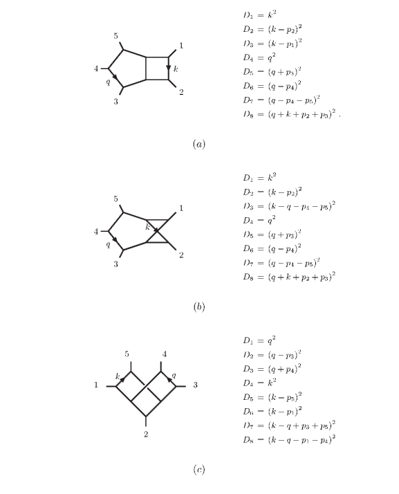
Figure 1: Five-point diagrams entering the amplitudes in $\mathcal{N}=4$ SYM and $\mathcal{N}=8$ SUGRA. They are the pentabox diagram $(a)$, the crossed pentabox diagram $(b)$ and the double pentagon diagram $(c)$. For each diagram, the definition of the denominators is shown as well.

3 Five-point amplitudes in ${\cal N}=4$ SYM

The five-point amplitude in ${\cal N}=4$ SYM can be expressed in terms of six diagrams [53]. The color ordered amplitude is given by a sum over the cyclic permutations of the external momenta. We apply the integrand reduction only to the three diagrams depicted in Fig. 1. The other three diagrams are trivially expressed in terms of scalar integrals, since their numerator is independent of the loop momenta. We consider one integrand at a time and we obtain its decomposition by evaluating its numerator on solutions of multiple cuts, i.e. on values of the loop momenta such that some of its denominators vanish.

We introduce the notation $\mathcal{I}^{(4,i)}$  ( $\mathcal{N}^{(4,i)}$) to denote the integrand (numerator) of the diagram in Fig. 1 $(i)$ in $\mathcal{N}=4$ SYM. The integrand of diagrams in Fig. 1 are

$${\cal I}^{(4,a)}_{1\cdots 8}(q,k)=\frac{{\cal N}^{(4,a)}_{1\cdots 8}(q,k)}{D_{1}\cdots D_{8}}\;, {\cal N}^{(4,a)}_{1\cdots 8}(q,k) =2\,q\cdot u_{1}+\beta_{1}\;,$$ (16)

$${\cal I}^{(4,b)}_{1\cdots 8}(q,k)=\frac{{\cal N}^{(4,b)}_{1\cdots 8}(q,k)}{D_{1}\cdots D_{8}}\;, {\cal N}^{(4,b)}_{1\cdots 8}(q,k) =2\,q\cdot u_{1}+\beta_{1}\;,$$ (17)

$${\cal I}^{(4,c)}_{1\cdots 8}(q,k)=\frac{{\cal N}^{(4,c)}_{1\cdots 8}(q,k)}{D_{1}\cdots D_{8}}\;, \mathcal{N}^{(4,c)}_{1\cdots 8}(q,k) =2\,q\cdot u_{2}+2\,k\cdot u_{3}+\beta_{2}+\beta_{3}\;,$$ (18)

The vectors $u_{1}^{\mu}$, $u_{2}^{\mu}$, and $u_{3}^{\mu}$ and the constants $\beta_{i}$ are defined as [53]

$$u_{1}^{\mu}= \frac{1}{4}\Big{(}\gamma_{35124}(p_{5}^{\mu}-p_{3}^{\mu})+\gamma_{34125}(p_{4}^{\mu}-p_{3}^{\mu})+\gamma_{45123}(p_{5}^{\mu}-p_{4}^{\mu})+2\,\gamma_{12345}(p_{2}^{\mu}-p_{1}^{\mu})\Big{)}\;,\quad$$ (19)

$$u_{2}^{\mu}= \frac{1}{4}\Big{(}\gamma_{23145}(p_{2}^{\mu}-p_{3}^{\mu})+\gamma_{24135}(p_{2}^{\mu}-p_{4}^{\mu})+\gamma_{34125}(p_{3}^{\mu}-p_{4}^{\mu})+2\,\gamma_{15234}(p_{1}^{\mu}-p_{5}^{\mu})\Big{)}\;,$$ (20)

$$u_{3}^{\mu}= \frac{1}{4}\Big{(}\gamma_{12345}(p_{1}^{\mu}-p_{2}^{\mu})+\gamma_{25134}(p_{2}^{\mu}-p_{5}^{\mu})+\gamma_{15234}(p_{1}^{\mu}-p_{5}^{\mu})+2\,\gamma_{34125}(p_{3}^{\mu}-p_{4}^{\mu})\Big{)}\;,$$ (21)

$$\beta_{1}= \frac{1}{4}\Big{(}\gamma_{35124}(s_{34}+s_{12}+s_{35})+2\,\gamma_{34125}\,s_{12}+\gamma_{45123}(s_{34}+s_{12}+s_{35})$$

$$+ 2\,\gamma_{12345}(s_{23}-s_{13})\Big{)}\;,$$ (22)

$$\beta_{2}= \frac{1}{4}\Big{(}-(\gamma_{23145}+\gamma_{24135})\,s_{23}+\gamma_{34125}(s_{15}+s_{34}+2\,s_{23})-2\,\gamma_{15234}(s_{13}-s_{35})\Big{)}\;,$$ (23)

$$\beta_{3}= \frac{1}{4}\Big{(}(\gamma_{12345}-\gamma_{25134})\,s_{12}+\gamma_{15234}(s_{34}+s_{15}+2\,s_{12})-2\,\gamma_{34125}(s_{13}-s_{14})\Big{)}\;.$$ (24)

where the kinematic invariants $s_{ij}$ and the functions $\gamma$ read as follows

$$s_{ij} \equiv(p_{i}+p_{j})^{2}=2\,(p_{i}\cdot p_{j})$$ (25)

$$\gamma_{12345} \equiv\left(\frac{[1\,2][2\,3][3\,4][4\,5][5\,1]}{[1\,4][2\,3]\langle 1\,2\rangle\langle 3\,4\rangle-[1\,2][3\,4]\langle 1\,4\rangle\langle 2\,3\rangle}\right)-\left(1\leftrightarrow 2\right).$$ (26)

In ${\cal N}=4$ SYM, given the simple form of the numerators, the multipole decomposition of the integrands only requires one iteration. The numerators can be decomposed as

$${\cal N}^{(4,x)}_{1\cdots 8}(q,k) = \Delta_{12345678}+\sum_{i=1}^{7}\Delta_{1\cdots(i-1)(i+1)\cdots 8}D_{i}\,\,\,,\,\,\,x=a,b,c\;.$$ (27)

The number of $7$-ple residues of the integrands ${\cal N}^{(4,a)}$ and ${\cal N}^{(4,b)}$ is almost halved since the numerator depends on $q$ only, thus $\Delta_{1\cdots(i-1)(i+1)\cdots 8}=0$ for $i\neq 4,5,6,7$.

In the next subsections, we list the parametrization of the residues entering our computation, namely of the residues in Eq. (27). All the eightfold residues are related to maximum cuts. According to the maximum-cut theorem [45], the number of coefficients needed to parametrize the residue of a maximum cut is finite and equal to the number of the solutions of the corresponding cut. We found the most general parametrization of the eightfold residue, which is process-independent and valid for numerators of any rank in both $q$ and $k$. The parametrization of the sevenfold residues is also process-independent and it is given for the case of renormalizable numerators of rank six at most, which is more than we need for the applications presented in this paper. The parametrization of higher rank numerators can be obtained including additional terms with higher powers of the loop momenta in the residues [54]. The number of coefficients required to parametrize the residues agrees with an independent computation performed using a technique based on Gram determinants.

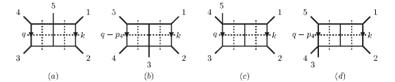
Figure 2: Cut diagrams of the sevenfold cuts. Starting from the left, we show the diagram of the cut $(1234568)$, $(1234678)$, $(1234578)$, and $(1235678)$.

cut	bases	${\mathbf{z}}$	Monomials in the residue
$(12345678)$	Eq. (28)	$(y_{4},y_{3},y_{2},y_{1},x_{4},x_{3},x_{2},x_{1})$	$\mathcal{S}_{12345678}=\{1,x_{1},y_{1},y_{2}\}$
$(1234568)$	Eq. (28)	$(y_{4},y_{3},y_{2},y_{1},x_{4},x_{3},x_{2},x_{1})$	$\mathcal{S}_{1234568}=\{1,x_{1},x_{1}^{2},x_{1}^{3},x_{1}^{4},x_{2},x_{1}x_{2},$
			$x_{1}^{2}x_{2},x_{1}^{3}x_{2},y_{1},x_{1}y_{1},x_{1}^{2}y_{1},x_{1}^{3}y_{1},x_{1}^{4}y_{1},$
			$x_{2}y_{1},x_{1}x_{2}y_{1},x_{1}^{2}x_{2}y_{1},x_{1}^{3}x_{2}y_{1},y_{1}^{2},x_{1}y_{1}^{2},$
			$x_{2}y_{1}^{2},y_{1}^{3},x_{1}y_{1}^{3},x_{2}y_{1}^{3},y_{1}^{4},x_{1}y_{1}^{4},x_{2}y_{1}^{4},y_{2},$
			$x_{1}y_{2},y_{1}y_{2},y_{1}^{2}y_{2},y_{1}^{3}y_{2}\}$
$(1234678)$	Eq. (28)	$(y_{4},y_{3},y_{2},y_{1},x_{4},x_{3},x_{2},x_{1})$	$\mathcal{S}_{1234678}=\mathcal{S}_{1234568}$
$(1234578)$	Eq. (29)	$(y_{4},y_{3},y_{2},y_{1},x_{4},x_{3},x_{2},x_{1})$	$\mathcal{S}_{1234578}=\{1,x_{2},x_{2}^{2},x_{2}^{3},x_{2}^{4},x_{4},x_{2}x_{4},$
			$x_{2}^{2}x_{4},x_{2}^{3}x_{4},y_{1},x_{2}y_{1},x_{2}^{2}y_{1},x_{2}^{3}y_{1},x_{2}^{4}y_{1},x_{4}y_{1},$
			$x_{2}x_{4}y_{1},x_{2}^{2}x_{4}y_{1},x_{2}^{3}x_{4}y_{1},y_{1}^{2},x_{2}y_{1}^{2},x_{4}y_{1}^{2},y_{1}^{3},x_{2}y_{1}^{3},$
			$x_{4}y_{1}^{3},y_{1}^{4},x_{2}y_{1}^{4},x_{4}y_{1}^{4},y_{4},x_{2}y_{4},y_{1}y_{4},$
			$y_{1}^{2}y_{4},y_{1}^{3}y_{4}\}$
$(1235678)$	Eq. (30)	$(y_{4},y_{3},y_{2},y_{1},x_{4},x_{3},x_{2},x_{1})$	$\mathcal{S}_{1235678}=\{1,x_{1},x_{1}^{2},x_{1}^{3},x_{1}^{4},x_{2},$
			$x_{1}x_{2},x_{1}^{2}x_{2},x_{1}^{3}x_{2},y_{1},x_{1}y_{1},x_{1}^{2}y_{1},$
			$x_{1}^{3}y_{1},x_{1}^{4}y_{1},x_{2}y_{1},x_{1}x_{2}y_{1},x_{1}^{2}x_{2}y_{1},x_{1}^{3}x_{2}y_{1},$
			$y_{1}^{2},x_{1}y_{1}^{2},x_{2}y_{1}^{2},y_{1}^{3},x_{1}y_{1}^{3},x_{2}y_{1}^{3},$
			$y_{1}^{4},x_{1}y_{1}^{4},x_{2}y_{1}^{4},y_{3},x_{1}y_{3},y_{1}y_{3},y_{1}^{2}y_{3},y_{1}^{3}y_{3}\}$

Table 1: Set of monomials parametrizing the residues entering the decomposition of the five-point pentabox diagram. They have all been found using degree lexicographic monomial ordering. For each cut the bases and the chosen ordering for loop variables are shown as well.

3.1 Residue of the planar pentabox

The decomposition of the pentabox diagram in Fig. 1 $(a)$ requires the parametrization of the residues of the eightfold cut $(12345678)$ and the sevenfold cuts depicted in Fig. 2. The parametrization is obtained using the procedure described in Section 2. The relevant bases are

$$\begin{cases}\begin{aligned} r_{0}^{\mu}&=0^{\mu},&e^{\mu}_{1}&=p_{3}^{\mu},&e^{\mu}_{2}&=p_{4}^{\mu},&e_{3}^{\mu}&=\frac{\langle 3|\gamma^{\mu}|4]}{2},&e_{4}^{\mu}&=\frac{\langle 4|\gamma^{\mu}|3]}{2},\quad\\ p_{0}^{\mu}&=0^{\mu},&\tau^{\mu}_{1}&=p_{2}^{\mu},&\tau^{\mu}_{2}&=p_{1}^{\mu},&\tau_{3}^{\mu}&=\frac{\langle 2|\gamma^{\mu}|1]}{2},&\tau_{4}^{\mu}&=\frac{\langle 1|\gamma^{\mu}|2]}{2},\quad\end{aligned}\\[21.52771pt] x_{1}=\frac{(q\cdot p_{1})}{(p_{1}\cdot p_{2})}\ ,\qquad x_{2}=\frac{(q\cdot p_{2})}{(p_{1}\cdot p_{2})}\ ,\qquad y_{1}=\frac{(k\cdot p_{4})}{(p_{3}\cdot p_{4})}\ ,\qquad y_{2}=\frac{(k\cdot p_{3})}{(p_{3}\cdot p_{4})}\ ;\end{cases}$$ (28)

$$\begin{cases}\begin{aligned} r_{0}^{\mu}&=0^{\mu},&e^{\mu}_{1}&=p_{1}^{\mu},&e^{\mu}_{2}&=p_{3}^{\mu},&e_{3,4}^{\mu}&=\frac{\langle 3|2|1]\langle 1|\gamma^{\mu}|3]\pm\langle 1|2|3]\langle 3|\gamma^{\mu}|1]}{4},\quad\\ p_{0}^{\mu}&=0^{\mu},&\tau^{\mu}_{1}&=p_{1}^{\mu},&\tau^{\mu}_{2}&=p_{3}^{\mu},&\tau^{\mu}_{3,4}&=\frac{\langle 3|2|1]\langle 1|\gamma^{\mu}|3]\pm\langle 1|2|3]\langle 3|\gamma^{\mu}|1]}{4},\quad\end{aligned}\\[21.52771pt] x_{1}=\frac{(q\cdot p_{3})}{(p_{1}\cdot p_{3})},\qquad x_{4}=\frac{(q\cdot\tau_{4})}{\tau_{4}^{2}},\qquad y_{1}=\frac{(k\cdot p_{3})}{(p_{1}\cdot p_{3})},\qquad y_{4}=\frac{(k\cdot e_{4})}{e_{4}^{2}};\end{cases}$$ (29)

$$\begin{cases}\begin{aligned} r_{0}^{\mu}&=0^{\mu},&e^{\mu}_{1,4}&=\frac{\langle 3|2|1]\langle 1|\gamma^{\mu}|3]\mp\langle 1|2|3]\langle 3|\gamma^{\mu}|1]}{4}&e^{\mu}_{2}&=p_{3}^{\mu},&e^{\mu}_{3}&=p_{1}^{\mu},\\ p_{0}^{\mu}&=-p_{4}^{\mu},&\tau^{\mu}_{1,4}&=\frac{\langle 3|2|1]\langle 1|\gamma^{\mu}|3]\mp\langle 1|2|3]\langle 3|\gamma^{\mu}|1]}{4},&\tau^{\mu}_{2}&=p_{3}^{\mu},&\tau^{\mu}_{3}&=p_{1}^{\mu},\end{aligned}\\[21.52771pt] x_{1}=\frac{((q-p_{4})\cdot e_{1})}{e_{1}^{2}},\qquad x_{2}=\frac{((q-p_{4})\cdot p_{1})}{(p_{1}\cdot p_{3})},\qquad y_{1}=\frac{(k\cdot\tau_{1})}{\tau_{1}^{2}},\qquad y_{3}=\frac{(k\cdot p_{3})}{(p_{1}\cdot p_{3})}.\qquad\end{cases}$$ (30)

The residue of each cut $(i_{1}\ldots i_{\kappa})$ is written in terms of a set of monomials $\mathcal{S}_{i_{1}\cdots i_{\kappa}}$, collected in Table 1.

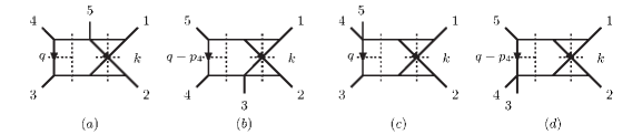
Figure 3: Cut diagrams of the sevenfold cuts. Starting from the left, we show the diagram of the cut $(1234568)$, $(1234678)$, $(1234578)$, and $(1235678)$.

cut	bases	${\mathbf{z}}$	Monomials in the residue
$(12345678)$	Eq. (28)	$(x_{4},x_{3},x_{2},y_{3},y_{4},x_{1},y_{2},y_{1})$	$\mathcal{S}_{12345678}=\{1,x_{1},y_{1},y_{2}\}$
$(1234568)$	Eq. (28)	$(y_{4},y_{3},y_{2},y_{1},x_{4},x_{3},x_{2},x_{1})$	$\mathcal{S}_{1234568}=\{1,x_{1},x_{1}^{2},x_{1}^{3},x_{1}^{4},x_{1}^{5},x_{1}^{6},x_{2},$
			$x_{1}x_{2},x_{1}^{2}x_{2},x_{1}^{3}x_{2},x_{1}^{4}x_{2},x_{1}^{5}x_{2},$
			$y_{1},x_{1}y_{1},x_{1}^{2}y_{1},x_{1}^{3}y_{1},x_{1}^{4}y_{1},x_{1}^{5}y_{1},x_{2}y_{1},$
			$x_{1}x_{2}y_{1},x_{1}^{2}x_{2}y_{1},x_{1}^{3}x_{2}y_{1},x_{1}^{4}x_{2}y_{1},y_{1}^{2},x_{1}y_{1}^{2},$
			$x_{2}y_{1}^{2},y_{1}^{3},x_{1}y_{1}^{3},x_{2}y_{1}^{3},y_{1}^{4},x_{1}y_{1}^{4},x_{2}y_{1}^{4},y_{2},$
			$x_{1}y_{2},y_{1}y_{2},y_{1}^{2}y_{2},y_{1}^{3}y_{2}\}$
$(1234678)$	Eq. (28)	$(y_{4},y_{3},y_{2},y_{1},x_{4},x_{3},x_{2},x_{1})$	$\mathcal{S}_{1234678}=\mathcal{S}_{1234568}$
$(1234578)$	Eq. (29)	$(y_{4},y_{3},y_{2},y_{1},x_{4},x_{3},x_{2},x_{1})$	$\mathcal{S}_{1234578}=\{1,x_{2},x_{2}^{2},x_{2}^{3},x_{2}^{4},x_{2}^{5},x_{2}^{6},x_{4},$
			$x_{2}x_{4},x_{2}^{2}x_{4},x_{2}^{3}x_{4},x_{2}^{4}x_{4},x_{2}^{5}x_{4},y_{1},x_{2}y_{1},$
			$x_{2}^{2}y_{1},x_{2}^{3}y_{1},x_{2}^{4}y_{1},x_{2}^{5}y_{1},x_{4}y_{1},x_{2}x_{4}y_{1},x_{2}^{2}x_{4}y_{1},$
			$x_{2}^{3}x_{4}y_{1},x_{2}^{4}x_{4}y_{1},y_{1}^{2},x_{2}y_{1}^{2},x_{4}y_{1}^{2},y_{1}^{3},x_{2}y_{1}^{3},$
			$x_{4}y_{1}^{3},y_{1}^{4},x_{2}y_{1}^{4},x_{4}y_{1}^{4},y_{4},x_{2}y_{4},y_{1}y_{4},y_{1}^{2}y_{4},y_{1}^{3}y_{4}\}$
$(1235678)$	Eq. (30)	$(y_{4},y_{2},y_{3},y_{1},x_{4},x_{3},x_{2},x_{1})$	$\mathcal{S}_{1235678}=\{1,x_{1},x_{1}^{2},x_{1}^{3},x_{1}^{4},x_{1}^{5},x_{1}^{6},x_{2},$
			$x_{1}x_{2},x_{1}^{2}x_{2},x_{1}^{3}x_{2},x_{1}^{4}x_{2},x_{1}^{5}x_{2},y_{1},$
			$x_{1}y_{1},x_{1}^{2}y_{1},x_{2}y_{1},x_{1}x_{2}y_{1},y_{1}^{2},x_{1}y_{1}^{2},x_{1}^{2}y_{1}^{2},$
			$x_{2}y_{1}^{2},x_{1}x_{2}y_{1}^{2},y_{1}^{3},x_{1}y_{1}^{3},x_{1}^{2}y_{1}^{3},x_{2}y_{1}^{3},x_{1}x_{2}y_{1}^{3},$
			$y_{1}^{4},x_{1}y_{1}^{4},x_{1}^{2}y_{1}^{4},x_{2}y_{1}^{4},x_{1}x_{2}y_{1}^{4},y_{3},x_{1}y_{3},$
			$y_{1}y_{3},y_{1}^{2}y_{3},y_{1}^{3}y_{3}\}$

Table 2: The same as Table 1, but for the five-point crossed pentabox diagram.

3.2 Residue of the crossed pentabox

The diagram in Fig. 1 $(b)$ is decomposed in terms of the residue of the eightfold cut $(12345678)$ and of the residue of the sevenfold cuts in Fig. 3. Each residue can be expressed in terms of a set of monomials, as shown in Table 2. The parametrization is obtained using the multivariate polynomial division described in Section 2.

cut	bases	${\mathbf{z}}$	Monomials in the residue
$(12345678)$	Eq. (33)	$(y_{4},y_{3},y_{2},y_{1},x_{4},x_{3},x_{1},x_{2})$	$\mathcal{S}_{12345678}=\{1,y_{1},x_{2},y_{1}x_{2},x_{2}^{2},x_{2}^{3},x_{1},x_{2}x_{1}\}$
$(1345678)$	Eq. (33)	$(x_{4},x_{3},x_{2},x_{1},y_{4},y_{3},y_{2},y_{1})$	$\mathcal{S}_{1345678}=\{1,y_{1},y_{1}^{2},y_{1}^{3},y_{1}^{4},y_{1}^{5},y_{1}^{6},y_{2},y_{1}y_{2},$
			$y_{1}^{2}y_{2},y_{1}^{3}y_{2},y_{1}^{4}y_{2},y_{1}^{5}y_{2},x_{1},$
			$y_{1}x_{1},y_{1}^{2}x_{1},y_{1}^{3}x_{1},y_{1}^{4}x_{1},y_{1}^{5}x_{1},$
			$y_{2}x_{1},y_{1}y_{2}x_{1},y_{1}^{2}y_{2}x_{1},y_{1}^{3}y_{2}x_{1},$
			$y_{1}^{4}y_{2}x_{1},x_{1}^{2},y_{1}x_{1}^{2},y_{2}x_{1}^{2},x_{1}^{3},y_{1}x_{1}^{3},$
			$y_{2}x_{1}^{3},x_{1}^{4},y_{1}x_{1}^{4},y_{2}x_{1}^{4},$
			$x_{2},y_{1}x_{2},x_{1}x_{2},x_{1}^{2}x_{2},x_{1}^{3}x_{2}\}$
$(1245678)$	Eq. (33)	$(x_{4},x_{3},x_{2},x_{1},y_{4},y_{3},y_{2},y_{1})$	$\mathcal{S}_{1245678}=\mathcal{S}_{1345678}$
$(2345678)$	Eq. (33)	$(x_{1},x_{3},x_{2},x_{4},y_{3},y_{4},y_{2},y_{1})$	$\mathcal{S}_{2345678}=\{1,y_{1},y_{1}^{2},y_{1}^{3},y_{1}^{4},y_{1}^{5},y_{1}^{6},y_{4},y_{1}y_{4},$
			$y_{1}^{2}y_{4},y_{1}^{3}y_{4},y_{1}^{4}y_{4},y_{1}^{5}y_{4},x_{2},y_{1}x_{2},$
			$x_{4},y_{1}x_{4},y_{1}^{2}x_{4},y_{1}^{3}x_{4},y_{1}^{4}x_{4},y_{1}^{5}x_{4},$
			$y_{4}x_{4},y_{1}y_{4}x_{4},y_{1}^{2}y_{4}x_{4},y_{1}^{3}y_{4}x_{4},$
			$y_{1}^{4}y_{4}x_{4},x_{2}x_{4},x_{4}^{2},y_{1}x_{4}^{2},y_{4}x_{4}^{2},$
			$x_{2}x_{4}^{2},x_{4}^{3},y_{1}x_{4}^{3},y_{4}x_{4}^{3},x_{2}x_{4}^{3},x_{4}^{4},y_{1}x_{4}^{4},y_{4}x_{4}^{4}\Big{\}}\;,$
$(1234567)$	Eq. (33)	$(x_{4},x_{3},x_{2},x_{1},y_{4},y_{3},y_{2},y_{1})$	$\mathcal{S}_{123567}=\{1,y_{1},y_{1}^{2},y_{1}^{3},y_{1}^{4},y_{2},y_{1}y_{2},y_{1}^{2}y_{2},y_{1}^{3}y_{2},$
			$x_{1},y_{1}x_{1},y_{1}^{2}x_{1},y_{1}^{3}x_{1},y_{1}^{4}x_{1},y_{2}x_{1},y_{1}y_{2}x_{1},$
			$y_{1}^{2}y_{2}x_{1},y_{1}^{3}y_{2}x_{1},x_{1}^{2},y_{1}x_{1}^{2},y_{2}x_{1}^{2},x_{1}^{3},$
			$y_{1}x_{1}^{3},y_{2}x_{1}^{3},x_{1}^{4},y_{1}x_{1}^{4},y_{2}x_{1}^{4},x_{2},y_{1}x_{2},$
			$x_{1}x_{2},x_{1}^{2}x_{2},x_{1}^{3}x_{2}\}$

Table 3: The same as Table 1, but for the five-point double pentagon diagram in Fig. 1 $(c)$.

3.3 Residue of the double pentagon

The decomposition of the double pentagon diagram requires the parametrization of the residues of the eightfold cut $(12345678)$ and all the sevenfold cuts. However, the topology in Fig. 1 $(c)$ is invariant under the transformation

$$p^{\mu}_{1}\leftrightarrow p^{\mu}_{3},\qquad p^{\mu}_{4}\leftrightarrow p^{\mu}_{5},\qquad q^{\mu}\leftrightarrow k^{\mu}\,;$$ (31)

thus the only sevenfold cut needed are $(1345678)$, $(1245678)$, $(2345678)$, and $(1234567)$, depicted in Fig. 4. The remaining sevenfold cuts can be obtained using the transformation (31). The eightfold cut is a maximum cut. It exhibits eight solutions and it is parametrized by eight coefficients, in accordance with the maxim-cut theorem.

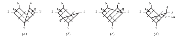
Figure 4: Cut diagrams of the sevenfold cuts. Starting from the left, we show the diagram of the cut $(1234567)$, $(1245678)$, $(1345678)$, and $(2345678)$.

The sets of monomials parametrizing the relevant residues are collected in Table 3. They are obtained by multivariate polynomial division using the following bases

$$\begin{cases}\begin{aligned} r_{0}^{\mu}&=0^{\mu},&e^{\mu}_{1}&=p_{4}^{\mu},&e^{\mu}_{2}&=p_{3}^{\mu},&e_{3}^{\mu}&=\frac{\langle 4|\gamma^{\mu}|3]}{2},&e_{4}^{\mu}&=\frac{\langle 3|\gamma^{\mu}|4]}{2},\quad\\ p_{0}^{\mu}&=0^{\mu},&\tau^{\mu}_{1}&=p_{5}^{\mu},&\tau^{\mu}_{2}&=p_{1}^{\mu},&\tau_{3}^{\mu}&=\frac{\langle 5|\gamma^{\mu}|1]}{2},&\tau_{4}^{\mu}&=\frac{\langle 1|\gamma^{\mu}|5]}{2},\quad\end{aligned}\\[21.52771pt] x_{1}=\frac{(q\cdot p_{1})}{(p_{5}\cdot p_{1})}\ ,\qquad x_{2}=\frac{(q\cdot p_{5})}{(p_{5}\cdot p_{1})}\ ,\qquad y_{1}=\frac{(k\cdot p_{3})}{(p_{3}\cdot p_{4})}\ ,\qquad y_{2}=\frac{(k\cdot p_{4})}{(p_{3}\cdot p_{4})}\ ;\end{cases}$$ (33)

$$\begin{cases}\begin{aligned} r_{0}^{\mu}&=0^{\mu},&e^{\mu}_{1}&=p_{1}^{\mu},&e^{\mu}_{2}&=p_{3}^{\mu},&e^{\mu}_{3,4}&=\frac{\langle 1|4|3]\langle 3|\gamma^{\mu}|1]\pm\langle 3|4|1]\langle 1|\gamma^{\mu}|3]}{4},\\ p_{0}^{\mu}&=-p_{3}^{\mu},&\tau^{\mu}_{1}&=p_{1}^{\mu},&\tau^{\mu}_{2}&=p_{3}^{\mu},&\tau_{3,4}^{\mu}&=\frac{\langle 1|4|3]\langle 3|\gamma^{\mu}|1]\pm\langle 3|4|1]\langle 1|\gamma^{\mu}|3]}{4},\\ \end{aligned}\\[21.52771pt] x_{2}=\frac{((q-p_{3})\cdot p_{1})}{(p_{1}\cdot p_{3})},\quad x_{4}=\frac{((q-p_{3})\cdot\tau_{4})}{\tau_{4}^{2}},\quad y_{1}=\frac{(k\cdot p_{3})}{(p_{1}\cdot p_{3})},\quad y_{4}=\frac{(k\cdot e_{4})}{e_{4}^{2}}.\end{cases}$$

4 Seminumerical integrand reduction

In the previous section we illustrated how to determine the general structure of the residues by means of the multivariate polynomial division. Knowing this structure, we can proceed and numerically perform the integrand reduction to extract the values of all process-dependent coefficients which appear in the residues. The decomposition can be checked by verifying the identity between the original numerator and its reconstruction, i.e. between l.h.s. and r.h.s. of Eq. (27), for arbitrary values of the integration momenta $q$ and $k$. This procedure is known as global $N=N$ test of the integrand reduction.

4.1 Planar pentabox diagram

Eightfold cut.

The residue of the eightfold cut can be parametrized using the monomials in Table 1:

$$\Delta_{12345678}=c_{12345678,\,0}+c_{12345678,\,1}(q\cdot p_{1})+c_{12345678,\,2}(k\cdot p_{3})+c_{12345678,\,3}(k\cdot p_{4})\,.$$ (34)

The number of solutions equals the number of coefficients, in accordance with the maximum-cut theorem. Therefore the four coefficients appearing in Eq. (34) can be obtained by sampling the numerator on the four solutions of the eightfold cut, where the decomposition (27) becomes

$${\cal N}^{(4,a)}_{1\cdots 8}=\Delta_{12345678}\;.$$ (35)

In our case we find that only $c_{12345678,\,0}$ and $c_{12345678,\,1}$ are nonvanishing.

Sevenfold cut.

The residue of the generic sevenfold cut $(i_{1}\cdots i_{7})$ appearing in Eq. (27) can be parametrized using the results listed in Table 1. For the process at hand, the structure of the numerator ensures that residue can be parametrized just by a constant term:

$$\Delta_{i_{1}\cdots i_{7}}=c_{i_{1}\cdots i_{7},\,0}\;.$$ (36)

The actual value of $c_{i_{1}\cdots i_{7},\,0}$ is obtained by sampling the numerator and the residue of the eightfold cut in correspondence of one solution of the sevenfold cut, where

$$\Delta_{i_{1}\cdots i_{7}}=\frac{{\cal N}^{(4,a)}_{1\cdots 8}(q,k)-\Delta_{12345678}}{\prod^{8}_{h\neq i_{1}\ldots i_{7}}D_{h}}\;.$$ (37)

The multipole decomposition of the integrand $\mathcal{I}^{(4,a)}_{1\cdots 8}$ becomes

$${\cal I}^{(4,a)}_{1\cdots 8}(q,k)=\frac{c_{12345678,\,0}+c_{12345678,\,1}(q\cdot p_{1})}{D_{1}\cdots D_{8}}+\sum_{i=4}^{7}\frac{c_{1\cdots(i-1)(i+1)\cdots 8,\,0}}{\prod_{h\neq i}^{8}D_{h}}\,.$$ (38)

This result also shows the decomposition of the integral as linear combination of two MIs with eight denominators and four MIs with seven denominators.

4.2 Crossed pentabox diagram

Eightfold cut.

The residue of the eightfold cut is parametrized as (cf. Table 2)

$$\Delta_{12345678}=c_{12345678,\,0}+c_{12345678,\,1}(q\cdot p_{1})+c_{12345678,\,2}(k\cdot p_{3})+c_{12345678,\,3}(k\cdot p_{4})\;.$$ (39)

The coefficients are obtained sampling the numerator at the four solutions of the maximum cut $(12345678)$, where

$${\cal N}^{(4,b)}_{1\cdots 8}=\Delta_{12345678}\;.$$ (40)

The only nonvanishing coefficients are $c_{12345678,\,0}$ and $c_{12345678,\,1}$.

Sevenfold cut.

The generic sevenfold cut appearing in the multipole decomposition of $\mathcal{I}_{1\cdots 8}^{(4,b)}$ is $(i_{1}\cdots i_{7})\in$ $\{(1234568),$ $(1234578),$ $(1234678),$ $(1235678)\}$. The structure of $\mathcal{N}^{(4,b)}_{1\cdots 8}$ guarantees that the only nonvanishing coefficient is the one of the monomial $1$, i.e.

$$\Delta_{i_{1}\cdots i_{7}}=c_{i_{1}\cdots i_{7},\,0}\;.$$ (41)

We sample the numerator and the residue of the eightfold cut at a solution of the cut $(i_{1}\cdots i_{7})$ and we get $c_{i_{1}\cdots i_{7},\,0}$ by using the relation

$$\Delta_{i_{1}\cdots i_{7}}=\frac{{\cal N}^{(4,a)}_{1\cdots 8}(q,k)-\Delta_{12345678}}{\prod^{8}_{h\neq i_{1}\ldots i_{7}}D_{h}}\;.$$ (42)

Within the numerical precision, the coefficients of the crossed pentabox turn out to be equal to the ones of the planar pentabox. This is expected since the two diagrams share the same numerator and also the denominators appearing in its decomposition are in common between the two.

The integrand $\mathcal{I}^{(4,b)}_{1\cdots 8}$ is decomposed as follows:

$${\cal I}^{(4,b)}_{1\cdots 8}(q,k)=\frac{c_{12345678,\,0}+c_{12345678,\,1}(q\cdot p_{1})}{D_{1}\cdots D_{8}}+\sum_{i=4}^{7}\frac{c_{1\cdots(i-1)(i+1)\cdots 8,\,0}}{\prod_{h\neq i}^{8}D_{h}}\,.$$ (43)

As for the previous diagram, this result yields the decomposition of the integral as linear combination of two MIs with eight denominators and four MIs with seven denominators.

4.3 Double pentagon diagram

Eightfold cut.

The parametrization of the residue of the eightfold cut is given in Table 3 and can be written as

$$\Delta_{12345678} = c_{12345678,\,0}+c_{12345678,\,1}(k\cdot p_{3})+c_{12345678,\,2}(q\cdot p_{5})$$ (44)

$$+ c_{12345678,\,3}(q\cdot p_{1})+c_{12345678,\,4}(q\cdot p_{5})^{2}+c_{12345678,\,5}(q\cdot p_{5})(q\cdot p_{1})$$

$$+ c_{12345678,\,6}(k\cdot p_{3})(q\cdot p_{5})+c_{12345678,\,7}(q\cdot p_{5})^{3}\,.$$

The eightfold cut is a maximum cut, thus the eight solutions of the eightfold cut allow one to determine the coefficients in Eq. (44) using the relation

$${\cal N}^{(4,b)}_{1\cdots 8}=\Delta_{12345678}\;,$$ (45)

which holds at the solutions of the eightfold cut. The nonvanishing coefficients are $c_{12345678,\,i}$ for $i\leq 4$.

Sevenfold cut.

The numerator has rank one and it is easy to see that the generic sevenfold residue $\Delta_{i_{1}\cdots i_{7}}$ entering Eq. (27) can be parametrized by a constant term, i.e.

$$\Delta_{i_{1}\cdots i_{7}}=c_{i_{1}\cdots i_{7},\,0}\;.$$ (46)

The value of $c_{i_{1}\cdots i_{7},\,0}$ is obtained by sampling the numerator and the residue of the eightfold cut at a solution of the cut $(i_{1}\cdots i_{7})$, where the relation

$$\Delta_{i_{1}\cdots i_{7}}=\frac{{\cal N}^{(4,c)}_{1\cdots 8}(q,k)-\Delta_{12345678}}{\prod^{8}_{h\neq i_{1}\ldots i_{7}}D_{h}}\;$$ (47)

holds. The multipole decomposition of the integrand of the double pentagon reads as follows

$${\cal I}^{(4,c)}_{1\cdots 8}(q,k) = \frac{c_{12345678,\,0}+c_{12345678,\,1}(k\cdot p_{3})}{D_{1}\cdots D_{8}}$$ (48)

$$+ \frac{c_{12345678,\,2}(q\cdot p_{5})+c_{12345678,\,3}(q\cdot p_{1})}{D_{1}\cdots D_{8}}$$

$$+ \sum_{i=1}^{8}\frac{c_{1\cdots(i-1)(i+1)\cdots 8,\,0}}{\prod_{h\neq i}^{8}D_{h}}\;.$$

The corresponding decomposition of the integral is a linear combination of four MIs with eight denominators and eight MIs with seven denominators.

4.4 Unitarity-based construction

In the previous subsections as well as in the following sections, we apply the multiloop integrand-reduction method in the case of integrands provided by a diagrammatic representation of the scattering amplitude, where the full dependence on the loop momenta is known. The method can, however, be applied also using a unitarity-based representation of the integrands, where the latter is known only in correspondence to multiple cuts in physical channels as a state sum over the product of tree-level amplitudes.

In this case, the integrand of the (color ordered) amplitude in $\mathcal{N}=4$ SYM reads as

$$\mathcal{I}^{(4)}(q,k)=\sum_{(i_{1}\cdots i_{8})}\frac{\Delta_{i_{1}\cdots i_{8}}}{D_{i_{1}}\cdots D_{i_{8}}}+\sum_{(i_{1}\cdots i_{7})}\frac{\Delta_{i_{1}\cdots i_{7}}}{D_{i_{1}}\cdots D_{i_{7}}}\,,$$ (49)

where the first (second) sum runs over all the eightfold (sevenfold) cuts.

The residue of the generic eightfold cut is given by

$$\Delta_{i_{1}\cdots i_{8}}=\mbox{Res}_{\,i_{1}\cdots i_{8}}\left\{\mathcal{I}^{(4)}\right\}\,,$$ (50)

where the (maximum-cut) residue $\mbox{Res}_{\,i_{1}\cdots i_{8}}\{\mathcal{I}^{(4)}\}$ is the state sum over the product of seven three-point tree-level amplitudes.

The residue of the generic sevenfold cut reads instead

$$\Delta_{i_{1}\cdots i_{7}}=\mbox{Res}_{\,i_{1}\cdots i_{7}}\left\{\mathcal{I}^{(4)}-\sum_{(i_{1}\cdots i_{8})}\frac{\Delta_{i_{1}\cdots i_{8}}}{D_{i_{1}}\cdots D_{i_{8}}}\right\}\,,$$ (51)

where $\mbox{Res}_{\,i_{1}\cdots i_{7}}\{\mathcal{I}^{(4)}\}$ is the state-sum product of six tree-level amplitudes, while the sum runs over all the sets $(i_{1}\cdots i_{8})$ containing $(i_{1}\cdots i_{7})$ as a subset.

The extension of the algorithm to lower cuts, if needed, is straightforward.

5 Five-point amplitudes in ${\cal N}=8$ SUGRA

The five-point amplitude in ${\cal N}=8$ SUGRA can be expressed in terms of the same six diagrams as in ${\cal N}=4$ SYM [53]. Again, the color ordered amplitude is given by a sum over the cyclic permutations of the external momenta. In ${\cal N}=8$ SUGRA, the numerator of each integrand is obtained by squaring the corresponding numerator in ${\cal N}=4$ SYM, as shown in [53]. We apply the integrand reduction only to the three diagrams depicted in Fig. 1, whose numerator exhibits a nontrivial dependence on the loop momenta. In the following we denote the integrand (numerator) of the diagram in Fig. 1 $(i)$ by $\mathcal{I}^{(8,i)}$ ( $\mathcal{N}^{(8,i)}$).

The numerators are of rank two in the loop momenta. Following the same machinery as in the case of ${\cal N}=4$ SYM, we show that their decomposition can be expressed in terms of 8-, 7-, and 6-denominator integrands:

$${\cal N}^{(8,x)}_{1\cdots 8}(q,k) = \Delta_{12345678}+\sum_{i=1}^{8}\Delta_{1\cdots(i-1)(i+1)\cdots 8}D_{i}$$ (52)

$$+\sum_{i<j=1}^{8}\Delta_{1\cdots(i-1)(i+1)\cdots(j-1)(j+1)\cdots 8}D_{i}D_{j}\,\,\,,\,\,\,x=a,b,c\;.$$

The corresponding decomposition for the integrands ${\cal I}^{(4,a)}_{1\cdots 8}$, ${\cal I}^{(4,b)}_{1\cdots 8}$ and ${\cal I}^{(4,c)}_{1\cdots 8}$ reads

$${\cal I}^{(4,x)}_{1\cdots 8}(q,k) = \frac{\Delta_{12345678}}{D_{1}\cdots D_{8}}+\sum_{i=1}^{8}\frac{\Delta_{1\cdots(i-1)(i+1)\cdots 8}}{\prod_{h\neq i}^{8}D_{h}}$$ (53)

$$+\sum_{i<j=1}^{8}\frac{\Delta_{1\cdots(i-1)(i+1)\cdots(j-1)(j+1)\cdots 8}}{\prod_{h\neq i,j}^{8}D_{h}}\,\,\,,\qquad\,\,\,x=a,b,c\;.$$

Since the numerators $\mathcal{N}^{(8,a)}_{1\cdots 8}$ and $\mathcal{N}^{(8,b)}_{1\cdots 8}$ are of rank two in $q$ and independent of $k$, their decomposition is significantly simplified. Indeed in these cases $\Delta_{1\cdots(i-1)(i+1)\cdots 8}=0$ for $i\neq 4,5,6,7$ and $\Delta_{1\cdots(i-1)(i+1)\cdots(j-1)(j+1)\cdots 8}=0$ for $i,j\neq 4,5,6,7$.

5.1 Seminumerical computation

In this section we briefly describe the numerical decomposition of the three numerators. We checked the decomposition by verifying that at arbitrary values of $q$ and $k$ the numerator and its reconstruction are equal.

Planar pentabox

Eightfold cut.

The computation of the residue of the eightfold cut $\Delta_{12345678}$ follows the same pattern as the $\mathcal{N}=4$ SYM planar pentabox, described in Section 4.1. The nonvanishing coefficients are $c_{12345678,\,0}$ and $c_{12345678,\,1}$.

Sevenfold cut.

The residue of the generic sevenfold cut $(i_{1}\cdots i_{7})$ in Eq. (52) can be parametrized in terms of the monomials collected in Table 1. The structure of the numerator guarantees that the residue contains rank-one terms at most:

$$\Delta_{i_{1}\cdots i_{7}} = c_{i_{1}\cdots i_{7},\,0}+c_{i_{1}\cdots i_{7},\,1}(q+w_{0})\cdot w_{1}+c_{i_{1}\cdots i_{7},\,2}(q+w_{0})\cdot w_{2}$$ (54)

$$+c_{i_{1}\cdots i_{7},\,3}(k+w_{3})\cdot w_{4}+c_{i_{1}\cdots i_{7},\,4}(k+w_{3})\cdot w_{5}\,.$$

The momenta $w^{\mu}_{i}$ depends on the cut $(i_{1}\cdots i_{7})$. The actual value of the coefficients can be obtained by sampling on five independent solutions of the sevenfold cut, where

$$\Delta_{i_{1}\cdots i_{7}}=\frac{{\cal N}^{(8,a)}_{1\cdots 8}(q,k)-\Delta_{12345678}}{\prod^{8}_{h\neq i_{1},\ldots,i_{7}}D_{h}}\;.$$ (55)

In this case, all the coefficients but $c_{i_{1}\cdots i_{7},\,0}$, $c_{i_{1}\cdots i_{7},\,1}$, and $c_{i_{1}\cdots i_{7},\,2}$ vanish.

Sixfold cut.

The numerator ${\cal N}^{(8,a)}_{1\cdots 8}$ has rank two in $q$ and is independent of $k$. The only nonvanishing term in the residue of the generic sixfold cut $(i_{1}\cdots i_{6})$ in (52) is the constant; therefore we have

$$\Delta_{i_{1}\cdots i_{6}} = c_{i_{1}\cdots i_{6},\,0}\,.$$ (56)

The actual value of the constant can be obtained evaluating the decomposition (52) at one solution of the sixfold cut, where

$$\Delta_{i_{1}\cdots i_{6}}=\frac{{\cal N}^{(8,a)}_{1\cdots 8}(q,k)-\Delta_{12345678}}{\prod^{8}_{h\neq i_{1},\ldots,i_{6}}D_{h}}-\sum_{h=4\atop h\neq i_{1},\ldots i_{6},}^{7}\frac{\Delta_{i_{1}\cdots h\cdots i_{6}}}{D_{h}}\;.$$ (57)

After polynomial fitting of $\Delta_{12345678}$, $\Delta_{i_{1}\cdots i_{7}}$ and $\Delta_{i_{1}\cdots i_{6}}$, the resulting multipole decomposition of Eq. (53) contains 20 nonvanishing coefficients two of which are spurious (i.e. their contribution vanishes upon integration) while the others give rise to MIs, namely two with eight denominators, ten with seven denominators and six with six denominators.

Crossed pentabox

As in the $\mathcal{N}=4$ SYM case, the crossed pentabox in Fig 1 $(b)$ has the same numerator and the same decomposition as the planar pentabox. Therefore the coefficients of the former are exactly the same as the coefficients of the latter.

Double pentagon

Eightfold cut.

The computation residue of the eightfold cut of the double pentagon follows the same lines of the $\mathcal{N}=4$ SYM double pentagon (see Section 4.3). The parametrization of the residue is given in Eq. (44). In this case the only vanishing coefficient is $c_{12345678,\,7}$.

Sevenfold cut.

The residue $\Delta_{i_{1}\cdots i_{7}}$ of the generic cut $(i_{1}\cdots i_{7})$ can be parametrized using Eq. (54). At the sevenfold cut $(i_{1}\cdots i_{7})$ the decomposition (52) reduces to

$$\Delta_{i_{1}\cdots i_{7}}=\frac{{\cal N}^{(8,c)}_{1\cdots 8}(q,k)-\Delta_{12345678}}{\prod^{8}_{h\neq i_{1},\ldots,i_{7}}D_{h}}\;.$$ (58)

The coefficients are then computed by sampling Eq. (58) at five solutions of the sevenfold cut. The nonvanishing ones are those multiplying constant or linear terms in the loop momenta.

Sixfold cut.

The residue $\Delta_{i_{1}\cdots i_{6}}$ of the generic sixfold cut $(i_{1}\cdots i_{6})$ can be parametrized by a constant, as in Eq. (56). The constant is computed using one solution of the sixfold cut and the expression of the decomposition (52) at the sixfold cut:

$$\Delta_{i_{1}\cdots i_{6}}=\frac{{\cal N}^{(8,a)}_{1\cdots 8}(q,k)-\Delta_{12345678}}{\prod^{8}_{h\neq i_{1},\ldots,i_{6}}D_{h}}-\sum_{h\neq i_{1},\ldots,i_{6}}^{8}\frac{\Delta_{i_{1}\cdots h\cdots i_{6}}}{D_{h}}\;.$$ (59)

We find that $\Delta_{123456}=0$, while the residues of all the other sixfold cuts are nonvanishing.

After polynomial fitting of $\Delta_{12345678}$, $\Delta_{i_{1}\cdots i_{7}}$ and $\Delta_{i_{1}\cdots i_{6}}$, the resulting multipole decomposition of Eq. (53) contains in this case 74 nonvanishing coefficients, four of which are spurious. The integral can be decomposed as a linear combination of seven MIs with eight denominators, 36 MIs with seven denominators and 27 MIs with six denominators.

6 Analytic integrand reduction

In this section we perform the reduction of the five-point diagrams analytically. We apply a two-loop generalization of the integrand reduction through Laurent expansion formulated in [54]. As in the one-loop case, the Laurent expansion allows one to find simpler formulas for the coefficients entering the decomposition. Moreover, the subtraction of the higher residues can be performed at the coefficient level rather than at the integrand level. Indeed the Laurent expansion makes each function entering the reduction separately polynomial. Therefore the subtraction can be omitted during the reduction and accounted for correcting the reconstructed coefficients. For simplicity we will focus on the rank-one numerators in the five-point integrands of ${\cal N}=4$ SYM. The method can, however, be extended to higher-rank numerators as described in Section 6.4 for the planar pentabox diagram in $\mathcal{N}=8$ SUGRA.

6.1 Planar pentabox diagram

The analytic decomposition of the pentabox diagram in Fig. 1 $(a)$ we are about to discuss, is valid for any numerator of the type (16), i.e. for any rank-one numerator depending on $q$ only. Indeed our computation is carried out for generic $u_{1}^{\mu}$ and $\beta_{1}$; the results for $\mathcal{N}=4$ SYM will be recovered at the very end, using Eqs. (19) and (22).

Eightfold cut.

The four solutions of the eightfold cut $(12345678)$ are

$$\left(q^{\mu}_{1},k^{\mu}_{1}\right)=\left(\frac{\langle 4\,5\rangle}{\langle 3\,5\rangle}\frac{\langle 3|\gamma^{\mu}|4]}{2},\;\frac{\langle 3\,2\rangle}{\langle 1\,3\rangle}\frac{\langle 1|\gamma^{\mu}|2]}{2}\right),\qquad \left(q^{\mu}_{2},k^{\mu}_{2}\right)=\left(\frac{\langle 4\,5\rangle}{\langle 3\,5\rangle}\frac{\langle 3|\gamma^{\mu}|4]}{2},\;\frac{\langle 1\,5\rangle}{\langle 2\,5\rangle}\frac{\langle 2|\gamma^{\mu}|1]}{2}\right),$$

$$\left(q^{\mu}_{3},k^{\mu}_{3}\right)=\left(\frac{[4\,5]}{[3\,5]}\frac{\langle 4|\gamma^{\mu}|3]}{2},\;\frac{[1\,5]}{[2\,5]}\frac{\langle 1|\gamma^{\mu}|2]}{2}\right),\qquad \left(q^{\mu}_{4},k^{\mu}_{4}\right)=\left(\frac{[4\,5]}{[3\,5]}\frac{\langle 4|\gamma^{\mu}|3]}{2},\;\frac{[3\,2]}{[1\,3]}\frac{\langle 2|\gamma^{\mu}|1]}{2}\right).$$

The general parametrization of the residue $\Delta_{12345678}$ is given in Eq. (34). The simple form of the numerator $\mathcal{N}^{(4,a)}_{1\cdots 8}$ implies that the coefficients $c_{12345678,\,2}$ and $c_{12345678,\,3}$ vanish. The nonvanishing coefficients are obtained by sampling at the solutions $(q_{1},k_{1})$ and $(q_{3},k_{3})$ only. The outcome is

$$c_{12345678,\,0} = -\frac{1}{\langle 5\,4\rangle\langle 3\,1\rangle[5\,3][4\,1]-\langle 5\,3\rangle\langle 4\,1\rangle[5\,4][3\,1]}$$ (60)

$$\quad\times\Big{(}\langle 5\,4\rangle\langle 4\,1\rangle\langle 3|u_{1}|4][5\,4][3\,1]-\langle 5\,4\rangle\langle 3\,1\rangle\langle 4|u_{1}|3][5\,4][4\,1]$$

$$\qquad-\beta_{1}\langle 5\,4\rangle\langle 3\,1\rangle[5\,3][4\,1]+\beta_{1}\langle 5\,3\rangle\langle 4\,1\rangle[5\,4][3\,1]\Big{)}$$

$$c_{12345678,\,1} = -2\frac{\langle 5\,4\rangle\langle 3|u_{1}|4][5\,3]-\langle 5\,3\rangle\langle 4|u_{1}|3][5\,4]}{\langle 5\,4\rangle\langle 3\,1\rangle[5\,3][4\,1]-\langle 5\,3\rangle\langle 4\,1\rangle[5\,4][3\,1]}.$$ (61)

Sevenfold cuts.

We discuss the generic sevenfold cut $(i_{1}\cdots i_{7})$ appearing the decomposition (27). For later convenience, we define the uncut propagator

$$D_{i_{8}}(q,k)=(q+P_{i_{8}})^{2},\quad\mbox{with}\;i_{8}\in\{1,\ldots,8\}\quad\mbox{and}\quad i_{8}\neq i_{1},\cdots,i_{7}.$$ (62)

The momentum $P^{\mu}_{i_{8}}$ is a linear combination of external momenta and it can be inferred from Fig. 1 $(a)$, for instance $P^{\mu}_{7}=-p^{\mu}_{4}-p^{\mu}_{5}$. The simplicity of the numerator allows one to parametrize the residue using the constant term $c_{i_{1}\cdots i_{7},\,0}$; cf. Eq. (36).

Every sevenfold cut of this topology exhibits a $t$-dependent family of solutions of the type

$$\left(q^{\mu}_{1},k^{\mu}_{1}\right) = \left(v^{\mu}_{q_{1},1}\,t+v^{\mu}_{q_{1},0},\;v^{\mu}_{k_{1}}\right)\;.$$ (63)

The coefficient $c_{i_{1}\cdot i_{7},\,0}$ can be computed evaluating Eq. (37) at the solutions (63). The computation can be simplified performing a Laurent expansion around $t=\infty$:

$$\left[\frac{\mathcal{N}^{(4,a)}_{1\cdots 8}(q_{1},k_{1})}{D_{i_{8}}(q_{1},k_{1})}-\frac{\Delta_{12345678}(q_{1},k_{1})}{D_{i_{8}}(q_{1},k_{1})}\right]_{t\to\infty}=c_{i_{1}\cdots i_{7},\,0}$$ (64)

Indeed in general neither

$$\frac{\mathcal{N}^{(4,a)}_{1\cdots 8}(q_{1},k_{1})}{D_{i_{8}}(q_{1},k_{1})}\qquad\mbox{nor}\qquad\frac{\Delta_{12345678}(q_{1},k_{1})}{D_{i_{8}}(q_{1},k_{1})}$$ (65)

are polynomial in $t$ but only their difference is. However, their truncated Laurent expansion obtained neglecting $\mathcal{O}(1/t)$ terms is polynomial in $t$, namely in this case a constant

$$\left.\frac{\mathcal{N}^{(4,a)}_{1\cdots 8}(q_{1},k_{1})}{D_{i_{8}}(q_{1},k_{1})}\right|_{t\to\infty}=n_{i_{1}\cdots i_{7},\,0}+\mathcal{O}\left(\frac{1}{t}\right),\qquad\left.\frac{\Delta_{12345678}(q_{1},k_{1})}{D_{i_{8}}(q_{1},k_{1})}\right|_{t\to\infty}=b_{i_{1}\cdots i_{7},\,0}+\mathcal{O}\left(\frac{1}{t}\right).\qquad$$ (66)

Therefore, similarly to the one-loop case [54], the coefficients $n_{i_{1}\cdots i_{7},\,0}$ and $b_{i_{1}\cdots i_{7},\,0}$ can be computed separately obtaining the coefficient $c_{i_{1}\cdots i_{7},\,0}$ by their difference:

$$c_{i_{1}\cdots i_{7},\,0}=n_{i_{1}\cdots i_{7},\,0}-b_{i_{1}\cdots i_{7},\,0}\;.$$ (67)

The subtraction can be performed at the coefficient level rather than at the integrand level. Moreover the known structure of $\Delta_{12345678}$ allows one to compute the coefficient $b_{i_{1}\cdots i_{7},\,0}$ once and for all, irrespective of the actual form of the numerator:

$$b_{i_{1}\cdots i_{7},\,0}=\frac{c_{12345678,\,1}(p_{1}\cdot v_{q_{1},1})}{2(P_{i_{8}}+v_{q_{1},0})\cdot v_{q_{1},1}}\;.$$ (68)

The coefficients $n_{i_{1}\cdots i_{7},\,0}$ read as follows:

$$n_{1234568,\,0}=-\frac{u_{1}\cdot v_{q_{1},1}}{p_{5}\cdot v_{q_{1},1}}\qquad \qquad v^{\mu}_{q_{1},1}=\frac{\langle 3|\gamma^{\mu}|4]}{2},$$ with

$$n_{1234678,\,0}=\frac{u_{1}\cdot v_{q_{1},1}}{p_{3}\cdot v_{q_{1},1}}\qquad \qquad v^{\mu}_{q_{1},1}=\frac{\langle 5|\gamma^{\mu}|4]}{2},$$ with

$$n_{1234578,\,0}=-\frac{u_{1}\cdot v_{q_{1},1}}{p_{4}\cdot v_{q_{1},1}}\qquad \qquad v^{\mu}_{q_{1},1}=\frac{\langle 3|\gamma^{\mu}|P_{345}]}{2},$$ with

$$n_{1235678,\,0}=-\frac{u_{1}\cdot v_{q_{1},1}}{p_{4}\cdot v_{q_{1},1}}\qquad \qquad v^{\mu}_{q_{1},1}=\frac{\langle 5|\gamma^{\mu}|P_{543}]}{2}.$$ with (69)

The massless momentum $P_{abc}$ is defined as

$$P_{abc}^{\mu}\equiv p_{b}^{\mu}+p_{c}^{\mu}-\frac{s_{bc}}{2(p_{b}+p_{c})\cdot p_{a}}p_{a}^{\mu}\;.$$ (70)

As already stated, the foregoing discussion applies to any numerator of the form given in Eq. (16). By using the explicit expressions of $u_{1}$ and $\beta_{1}$ given in Eqs. (19) and (22), we can write down the results for the coefficients in $\mathcal{N}=4$ SYM in terms of the functions $\gamma$ defined in Eq (26)

$$c_{12345678,\,0}={} \frac{1}{2}\left(\gamma_{12345}(s_{23}-s_{13}-s_{45})+s_{12}(\gamma_{34125}+\gamma_{35124}+\gamma_{45123})\right)$$

$$c_{12345678,\,1}={} -2\,\gamma_{12345}$$

$$c_{1234568,\,0}={} \frac{1}{4}(-\gamma_{35124}-\gamma_{45123}+2\,\gamma_{12345})$$

$$c_{1234578,\,0}={} \frac{1}{4}(-\gamma_{34125}+\gamma_{35124}+2\,\gamma_{45123})$$

$$c_{1234678,\,0}={} \frac{1}{4}(-\gamma_{35124}-\gamma_{34125}-2\,\gamma_{12345})$$

$$c_{1235678,\,0}={} \frac{1}{4}(-\gamma_{45123}+\gamma_{35124}+2\,\gamma_{34125}).$$ (71)

The complete integrand decomposition is obtained plugging the coefficients of Eq. (6.1) in Eq. (38). These results are in agreement with the ones found in the numerical computation of Section 4.1.

6.2 Crossed pentabox diagram

As already noticed in Section 4.2, the crossed pentabox of Fig. 1 $(b)$ and the planar pentabox have the same decomposition. Indeed the numerator $\mathcal{N}^{(4,a)}_{1\cdots 8}$ and the numerator $\mathcal{N}^{(4,b)}_{1\cdots 8}$, Eq. (17), are equal and are decomposed in terms of the same denominators; cf. Eqs. (43) and (38) multiplied by $D_{i_{1}}\ldots D_{i_{8}}$. Therefore the coefficients appearing in the multipole decomposition (43) are equal to the corresponding ones appearing in the decomposition (38) of the planar pentabox.

6.3 Double pentagon diagram

The numerator $\mathcal{N}^{(4,c)}_{1\cdots 8}$, Eq. (18), is highly symmetric in $q$ and $k$. Indeed the dependence on $q$ and $k$ can be disentangled and $\mathcal{N}^{(4,c)}_{1\cdots 8}$ can be cast in the following form:

$$\mathcal{N}^{(4,c)}_{1\cdots 8}(q,k)=\mathcal{R}^{(4,c)}_{1\cdots 8}(q)-\mathcal{T}^{(4,c)}_{1\cdots 8}(k)\,,$$ (72)

where

$$\mathcal{R}^{(4,c)}_{1\cdots 8}(\ell)\equiv 2\ell\cdot u_{2}+\beta_{2},\qquad\mathcal{T}^{(4,c)}_{1\cdots 8}(k)=\mathcal{R}^{(4,c)}_{1\cdots 8}(k)\,|_{p_{1}\leftrightarrow p_{3},\,p_{4}\leftrightarrow p_{5}}\;$$ (73)

The vector $u_{2}$ and the constant $\beta_{2}$ are defined in Eqs. (20) and (23), respectively. Although in principle there are no additional issues in performing the reduction of the full numerator, the computation can be simplified by performing the reduction of $\mathcal{R}^{(4,c)}_{1\cdots 8}(q)$ only. The reduction of $\mathcal{T}^{(4,c)}_{1\cdots 8}(q)$, and thus of the full numerator $\mathcal{N}^{(4,c)}_{1\cdots 8}(q,k)$, is then obtained by means of the substitutions (31). The numerator $\mathcal{R}^{(4,c)}_{1\cdots 8}(q)$ depends on $q$ only and can be decomposed as follows:

$$\mathcal{R}^{(4,c)}_{1\cdots 8}(q)=\Delta_{12345678}+\sum_{i=1}^{3}\Delta_{1\cdots(i-1)(i+1)\cdots 8}D_{i}\;.$$ (74)

Eightfold cut.

The solutions of the eightfold cut $(12345678)$ are eight and they can be used to compute the eight coefficients parametrizing the residue

$$\Delta_{12345678} = \hat{c}_{12345678,\,0}+\hat{c}_{12345678,\,1}(k\cdot p_{3})+\hat{c}_{12345678,\,2}(q\cdot p_{5})$$ (75)

$$+ \hat{c}_{12345678,\,3}(q\cdot p_{1})+\hat{c}_{12345678,\,4}(q\cdot p_{5})^{2}+\hat{c}_{12345678,\,5}(q\cdot p_{5})(q\cdot p_{1})$$

$$+ \hat{c}_{12345678,\,6}(k\cdot p_{3})(q\cdot p_{5})+\hat{c}_{12345678,\,7}(q\cdot p_{5})^{3}\;.$$

The rank of $\mathcal{R}^{(4,c)}_{1\cdots 8}$ implies that for $i\geq 4$ $\hat{c}_{12345678,\,i}=0$. The simplicity of the numerator simplifies the computation even further. Indeed decomposing $u_{2}^{\mu}$ in the basis $\{p_{i}\}_{i=1,\cdots,4}$, and using the conditions $D_{1}=D_{2}=D_{3}=0$ we get

$$\hat{c}_{12345678,\,0}=\beta_{2},\qquad\hat{c}_{12345678,\,1}=0\;.$$ (76)

The two remaining coefficients can be obtained by sampling the numerator on two solutions of the eightfold cut, e.g.

$$(k_{1}^{\mu},q_{1}^{\mu}) = \left(\frac{\langle 4\,1\rangle}{\langle 4\,5\rangle}\frac{\langle 5|\gamma^{\mu}|1]}{2},\;\frac{\langle 3\,5\rangle}{\langle 4\,5\rangle}\,\frac{\langle 4|\gamma^{\mu}|3]}{2}\right)\,,$$

$$(k_{2}^{\mu},q_{2}^{\mu}) = \left(\frac{[4\,1]}{[4\,5]}\,\frac{\langle 1|\gamma^{\mu}|5]}{2},\;\frac{[3\,5]}{[4\,5]}\frac{\langle 3|\gamma^{\mu}|4]}{2}\right)\,.$$

The missing coefficients read as follows:

$$\hat{c}_{12345678,\,2}=-2\frac{\langle 4|1|3]\langle 3|u_{2}|4]-\langle 3|1|4]\langle 4|u_{2}|3]}{\langle 4|5|3]\langle 3|1|4]-\langle 3|5|4]\langle 4|1|3]}\,,$$

$$\hat{c}_{12345678,\,3}=2\frac{\langle 4|5|3]\langle 3|u_{2}|4]-\langle 3|5|4]\langle 4|u_{2}|3]}{\langle 4|5|3]\langle 3|1|4]-\langle 3|5|4]\langle 4|1|3]}.$$ (77)

Sevenfold cuts.

We consider the generic sevenfold cut $(i_{1}\cdots i_{7})$ appearing in the decomposition (74). The solutions of the cut can be cast into one-parameter families. In particular each cut allows for a solution with the following asymptotic behavior

$$(k_{1}^{\mu},\;q_{1}^{\mu})=\left(v_{k_{1},1}^{\mu}t+v_{k_{1},0}^{\mu}+\mathcal{O}\left(\frac{1}{t}\right),\;v_{q_{1},1}^{\mu}t+v_{q_{1},0}^{\mu}+\mathcal{O}\left(\frac{1}{t}\right)\right)\qquad\mbox{for}\;t\to\infty\,.$$ (78)

We compute the coefficient $\hat{c}_{1345678,\,0}$ by evaluating the decomposition (74) at one solution of the sevenfold cut, and by expanding around $t=\infty$:

$$\left[\frac{\mathcal{R}^{(4,c)}_{1\cdots 8}(q_{1})}{D_{i_{8}}(q_{1},k_{1})}-\frac{\Delta_{12345678}(q_{1},k_{1})}{D_{i_{8}}(q_{1},k_{1})}\right]_{t\to\infty}=\hat{c}_{i_{1}\cdots i_{7},\,0}\;.$$ (79)

The denominator $D_{i_{8}}$ is written in terms of $P_{i_{8}}^{\mu}$ as in Eq. (62). The actual form of $P_{i_{8}}^{\mu}$ is inferred from Fig. 1 $(c)$. Also in this case the $t\to\infty$ limit makes both

$$\frac{\mathcal{R}^{(4,c)}_{1\cdots 8}(q_{1})}{D_{i_{8}}(q_{1},k_{1})}\qquad\mbox{and}\qquad\frac{\Delta_{12345678}(q_{1},k_{1})}{D_{i_{8}}(q_{1},k_{1})}$$ (80)

polynomial in $t$,

$$\left.\frac{\mathcal{R}^{(4,c)}_{1\cdots 8}(q_{1})}{D_{i_{8}}(q_{1},k_{1})}\right|_{t\to\infty}=\hat{n}_{i_{1}\cdots i_{7},\,0}+\mathcal{O}\left(\frac{1}{t}\right),\qquad\left.\frac{\Delta_{12345678}(q_{1},k_{1})}{D_{i_{8}}(q_{1},k_{1})}\right|_{t\to\infty}=\hat{b}_{i_{1}\cdots i_{7},\,0}+\mathcal{O}\left(\frac{1}{t}\right).$$ (81)

The coefficients $\hat{n}_{i_{1}\cdots i_{7},\,0}$ and $\hat{b}_{i_{1}\cdots i_{7},\,0}$ can be computed separately, and

$$\hat{c}_{i_{1}\cdots i_{7},\,0}=\hat{n}_{i_{1}\cdots i_{7},\,0}-\hat{b}_{i_{1}\cdots i_{7},\,0}\;.$$ (82)

Therefore the subtraction can be performed at the coefficient level via the universal function

$$\hat{b}_{i_{1}\cdots i_{7},\,0}=\frac{\hat{c}_{12345678,\,2}(v_{q_{1},1}\cdot p_{5})+\hat{c}_{12345678,\,3}(v_{q_{1},1}\cdot p_{1})}{2(v_{q_{1},0}+P_{i_{8}})\cdot v_{q_{1},1}}\;.$$ (83)

The coefficients $\hat{n}_{i_{1}\cdots i_{7},\,0}$ are given by

$$\hat{n}_{1345678,\,0}=-\frac{u_{2}\cdot v_{q_{1}}}{p_{3}\cdot v_{q_{1}}},\quad \quad v^{\mu}_{q_{1}}=\eta_{1}\frac{\langle 4|\gamma^{\mu}|3]}{2}+\eta_{2}p_{4}^{\mu},$$ with

$$\hat{n}_{1245678,\,0}=\frac{u_{2}\cdot v_{q_{1}}}{p_{4}\cdot v_{q_{1}}},\quad \quad v^{\mu}_{q_{1}}=\eta_{3}\frac{\langle 4|\gamma^{\mu}|3]}{2}+\eta_{4}p_{3}^{\mu},$$ with

$$\hat{n}_{1234578,\,0}=\frac{u_{2}\cdot v_{q_{1}}}{p_{3}\cdot v_{q_{1}}},\quad \quad v^{\mu}_{q_{1}}=\eta_{5}(p_{3}^{\mu}-p_{4}^{\mu})+\eta_{6}\frac{\langle 3|\gamma^{\mu}|4]}{2}+\eta_{7}\frac{\langle 4|\gamma^{\mu}|3]}{2}.$$ with (84)

We define

$$\eta_{1} = -\frac{\langle 5\,2\rangle[4\,1]}{\langle 4\,2\rangle[3\,4]}\,,$$

$$\eta_{2} = \frac{\langle 5\,2\rangle[3\,1]}{\langle 4\,2\rangle[3\,4]}\,,$$

$$\eta_{3} = \frac{\langle 3\,5\rangle[1\,2]}{\langle 3\,4\rangle[3\,2]}\,,$$

$$\eta_{4} = -\frac{\langle 4\,5\rangle[1\,2]}{\langle 3\,4\rangle[3\,2]}\,,$$

$$\eta_{5} = \frac{-\sigma_{1}+\sqrt{\sigma_{1}^{2}-4\sigma_{2}\sigma_{3}}}{2\sigma_{2}}\,,$$

$$\eta_{6} = \frac{2\sigma_{2}\sigma_{8}-\sigma_{1}\sigma_{4}+\sigma_{4}\sqrt{\sigma_{1}^{2}-4\sigma_{2}\sigma_{3}}}{2\sigma_{2}\sigma_{5}}\,,$$

$$\eta_{7} = -\frac{2\sigma_{2}\sigma_{7}-\sigma_{1}\sigma_{6}+\sigma_{6}\sqrt{\sigma_{1}^{2}-4\sigma_{2}\sigma_{3}}}{2\sigma_{2}\sigma_{5}}\,,$$ (85)

in terms of

$$\sigma_{1}={} -4(\sigma_{7}\sigma_{4}+\sigma_{6}\sigma_{8})(p_{1}\cdot p_{2})\,,$$

$$\sigma_{2}={} -4(\sigma_{6}\sigma_{4}-\sigma_{5}^{2})(p_{1}\cdot p_{2})\,,$$

$$\sigma_{3}={} -4\sigma_{7}\sigma_{8}(p_{1}\cdot p_{2})\,,$$

$$\sigma_{4}={} 2(p_{1}\cdot p_{5})\langle 4\,5\rangle[3\,1]-2(p_{2}\cdot p_{5})\langle 4\,5\rangle[3\,1]+\langle 3\,5\rangle\langle 4\,2\rangle[3\,1][3\,2]-\langle 4\,5\rangle\langle 4\,2\rangle[3\,2][4\,1]\,,$$

$$\sigma_{5}={} -\langle 3\,5\rangle\langle 4\,2\rangle[3\,2][4\,1]+\langle 3\,2\rangle\langle 4\,5\rangle[3\,1][4\,2]\,,$$

$$\sigma_{6}={} 2(p_{2},\cdot p_{3})\langle 3\,5\rangle[4\,1]-2(p_{2}\cdot p_{5})\langle 3\,5\rangle[4\,1]+\langle 3\,5\rangle\langle 3\,2\rangle[3\,1][4\,2]-\langle 3\,2\rangle\langle 4\,5\rangle[4\,1][4\,2]\,,$$

$$\sigma_{7}={} \langle 3\,5\rangle\langle 5\,2\rangle[4\,1][1\,2]\,,$$

$$\sigma_{8}={} \langle 4\,5\rangle\langle 5\,2\rangle[3\,1][1\,2].$$ (86)

This completes the reduction of a generic numerator $\mathcal{R}^{(4,c)}_{1\cdots 8}$ of the form given in Eq. (73). As previously stated, the reduction of the full numerator $\mathcal{N}^{(4,c)}_{1\cdots 8}$ of $\mathcal{N}=4$ SYM can be recovered from the one discussed in this section, by means of Eqs. (72) and (73). To that purpose, we observe that the substitutions (31) give the one-to-one mapping between denominators

$$D_{1}\leftrightarrow D_{4},\qquad D_{2}\leftrightarrow D_{6},\qquad D_{3}\leftrightarrow D_{5},\qquad D_{7}\leftrightarrow D_{8}.$$

Putting everything together and using the definitions of $u_{2}$ and $\beta_{2}$ of Eqs. (20) and (23) we recover the full multipole decomposition of Eq. (48), with coefficients

$$c_{12345678,\,0} =\frac{1}{4}\Big{(}\gamma_{34125}(2s_{13}-2s_{35}+2s_{23}+s_{15}+s_{34})$$

$$\qquad-\gamma_{15234}(2s_{13}-2s_{35}+2s_{12}+s_{15}+s_{34})$$

$$\qquad-(\gamma_{23145}+\gamma_{24135})\,s_{23}-(\gamma_{25134}-\gamma_{12345})(s_{35}-s_{14}-s_{12})\Big{)}\,,$$

$$c_{12345678,\,1} =-2\,\gamma_{34125}\,,$$

$$c_{12345678,\,2} =\frac{1}{2}(2\gamma_{34125}-\gamma_{23145}-\gamma_{24135}-2\gamma_{15234}+\gamma_{25134}-\gamma_{12345})\,,$$

$$c_{12345678,\,3} =\frac{1}{2}(2\gamma_{34125}-\gamma_{23145}-\gamma_{24135}+2\gamma_{15234}+\gamma_{25134}-\gamma_{12345})\,,$$

$$c_{2345678,\,0} =\frac{1}{4}(2\gamma_{34125}-\gamma_{23145}+\gamma_{24135})\,,$$

$$c_{1345678,\,0} =\frac{1}{4}(-3\gamma_{34125}+2\gamma_{23145}+\gamma_{24135}-\gamma_{25134}+\gamma_{12345})\,,$$

$$c_{1245678,\,0} =\frac{1}{4}(\gamma_{34125}-\gamma_{23145}-2\gamma_{24135}+\gamma_{25134}-\gamma_{12345})\,,$$

$$c_{1235678,\,0} =\frac{1}{4}(-2\gamma_{15234}-\gamma_{25134}-\gamma_{12345})\,,$$

$$c_{1234678,\,0} =\frac{1}{4}(-2\gamma_{34125}+\gamma_{15234}+\gamma_{25134})\,,$$

$$c_{1234578,\,0} =\frac{1}{4}(2\gamma_{34125}+\gamma_{15234}+\gamma_{12345})\,,$$

$$c_{1234568,\,0} =\frac{1}{4}(2\gamma_{34125}+\gamma_{25134}-\gamma_{12345})\,,$$

$$c_{1234567,\,0} =\frac{1}{4}(-2\gamma_{34125}-\gamma_{25134}+\gamma_{12345}).$$ (87)

The coefficients of Eq. (87) enter the integrand decomposition of Eq. (48). These results are in agreement with the numerical computation of Section 4.3.

6.4 Higher-rank integrands

The analytic reduction via Laurent expansion can be extended to numerators of higher rank. As an example we perform the computation of the sevenfold residues for the $\mathcal{N}=8$ SUGRA two-loop five-points planar pentabox, whose numerator has rank two in the loop momentum $q$.

The most general parametrization of the residue of the generic sevenfold cut $(i_{1}\cdots i_{7})$ is

$$\Delta_{i_{1}\cdots i_{7}}(q,k)=c_{i_{1}\cdots i_{7},\,0}+c_{i_{1}\cdots i_{7},\,1}(q+w_{0})\cdot w_{1}+c_{i_{1}\cdots i_{7},\,2}(q+w_{0})\cdot w_{2}.$$ (88)

The momenta $w_{0}^{\mu}$, $w_{1}^{\mu}$, and $w^{\mu}_{2}$ are a linear combination of the external momenta and depend on the cut $(i_{1}\cdots i_{7})$. Their actual form is not relevant for this discussion but can be inferred from Table 2. We consider two $t$-dependent solutions of the sevenfold cut:

$$(q_{i}^{\mu},k_{i}^{\mu})=\left(v^{\mu}_{q_{i},1}t+v^{\mu}_{q_{i},0},\;v^{\mu}_{k_{i}}\right)\quad\mbox{with}\quad=1,2\;.$$ (89)

The coefficients in Eq. (88) can be computed evaluating (52) at the solutions (89)

$$\frac{\mathcal{N}^{(8,a)}_{1\cdots 8}(q_{i},k_{i})-\Delta_{12345678}(q_{i},k_{i})}{D_{i_{8}}(q_{i},k_{i})} = \Delta_{i_{1}\cdots i_{7}}(q_{i},k_{i})$$ (90)

$$= c_{i_{1}\cdots i_{7},\,0}+c_{i_{1}\cdots i_{7},\,1}(v_{q_{i},0}+w_{0})\cdot w_{1}$$

$$+c_{i_{1}\cdots i_{7},\,2}(v_{q_{i},0}+w_{0})\cdot w_{2}+c_{i_{1}\cdots i_{7},\,1}(v_{q_{i},1}\cdot w_{1})t$$

$$+c_{i_{1}\cdots i_{7},\,2}(v_{q_{i},1}\cdot w_{2})t,\qquad$$

where $D_{i_{8}}$ is defined in Eq. (62). The Laurent expansion around $t=\infty$ simplifies the computation. Indeed in this limit both

$$\frac{\mathcal{N}^{(8,a)}_{1\cdots 8}(q_{i},k_{i})}{D_{i_{8}}(q_{i},k_{i})}\qquad\mbox{and}\qquad\frac{\Delta_{12345678}(q_{i},k_{i})}{D_{i_{8}}(q_{i},k_{i})}$$ (91)

have the same polynomial structure of the residue:

$$\left.\frac{\mathcal{N}^{(8,a)}_{1\cdots 8}(q_{i},k_{i})}{D_{i_{8}}(q_{i},k_{i})}\right|_{t\to\infty} = n_{i_{1}\cdots i_{7},\,0}^{[i]}+n_{i_{1}\cdots i_{7},\,1}^{[i]}t+\mathcal{O}\left(\frac{1}{t}\right)$$

$$\left.\frac{\Delta_{12345678}(q_{i},k_{i})}{D_{i_{8}}(q_{i},k_{i})}\right|_{t\to\infty} = b_{i_{1}\cdots i_{7},\,0}^{[i]}+\mathcal{O}\left(\frac{1}{t}\right)\;.$$ (92)

The expression of the coefficients is obtained by plugging the expansions (92) in Eq. (90) and by comparing both sides. In particular $c_{i_{1}\cdots i_{7},\,1}$ and $c_{i_{1}\cdots i_{7},\,2}$ are the solution of the system

$$\left\{\begin{array}[]{r l}c_{i_{1}\cdots i_{7},\,1}(v_{q_{1}}\cdot w_{1})+c_{i_{1}\cdots i_{7},\,2}(v_{q_{1}}\cdot w_{2})&=n_{i_{1}\cdots i_{7},\,1}^{[1]}\\[8.61108pt] c_{i_{1}\cdots i_{7},\,1}(v_{q_{2}}\cdot w_{1})+c_{i_{1}\cdots i_{7},\,2}(v_{q_{2}}\cdot w_{2})&=n_{i_{1}\cdots i_{7},\,1}^{[2]}\\ \end{array}\right..$$ (93)

The coefficient $c_{i_{1}\cdots i_{7},\,0}$ is given by

$$c_{i_{1}\cdots i_{7},\,0} = n_{i_{1}\cdots i_{7},\,0}^{[1]}-b_{i_{1}\cdots i_{7},\,0}^{[1]}-c_{i_{1}\cdots i_{7},\,1}(v_{q_{1},0}+w_{0})\cdot w_{1}-c_{i_{1}\cdots i_{7},\,2}(v_{q_{1},0}+w_{0})\cdot w_{2}$$ (94)

$$= n_{i_{1}\cdots i_{7},\,0}^{[2]}-b_{i_{1}\cdots i_{7},\,0}^{[2]}-c_{i_{1}\cdots i_{7},\,1}(v_{q_{2},0}+w_{0})\cdot w_{1}-c_{i_{1}\cdots i_{7},\,2}(v_{q_{2},0}+w_{0})\cdot w_{2},\qquad$$

in terms of the functions

$$b_{i_{1}\cdots i_{7},\,0}^{[i]}=\frac{c_{12345678,\,1}(p_{1}\cdot v_{q_{i},1})}{2(v_{q_{i},0}+P_{i_{8}})\cdot v_{q_{i},1}}\;.$$ (95)

Eq. (94) shows that the coefficient $c_{i_{1}\cdots i_{7},\,0}$ can be written as the constant term $n_{i_{1}\cdots i_{7},\,0}^{[i]}$ of the Laurent expansion of the integrand, corrected by two kinds of contributions. The first, $b_{i_{1}\cdots i_{7},\,0}^{[i]}$, implements the eightfold-cut subtraction as a correction at the coefficient level. The other terms are proportional to the higher-rank coefficients of the same cut found as solutions of the system in Eq. (93).

7 Conclusions

We recently proposed a new approach for the reduction of scattering amplitudes [45], based on multivariate polynomial division. This technique yields the complete integrand decomposition for arbitrary amplitudes, regardless of the number of loops. In particular it allows for the determination of (the polynomial form of) the residue at any multiparticle cut, whose knowledge is a mandatory prerequisite for applying the integrand-reduction procedure. We have also shown how the shape of the residues is uniquely determined by the on-shell conditions and, by using the division modulo Gröbner basis, we have derived a simple integrand recurrence relation generating the multiparticle pole decomposition for arbitrary multiloop amplitudes.

In the present paper, we applied the new reduction algorithm to planar and non planar diagrams appearing in the two-loop five-point amplitudes in $\mathcal{N}=4$ SYM and $\mathcal{N}=8$ SUGRA (in four dimensions), whose numerator functions contain up to rank-two terms in the integration momenta. We determined all polynomial residues parametrizing the cuts of the corresponding topologies and subtopologies. At the same time, the polynomial form of the residues defines the integral basis for the amplitude decomposition. For the considered cases, we found that the amplitude can be decomposed in terms of independent integrals with eight, seven, and six denominators.

Our presented approach is well suited for a seminumerical implementation. The mathematical framework it is based on is very general and provides an effective algorithm for the generalization of the integrand-reduction method to all orders in perturbation theory.

References

- [1] Z. Bern, L. J. Dixon, D. C. Dunbar, and D. A. Kosower, One-Loop n-Point Gauge Theory Amplitudes, Unitarity and Collinear Limits, Nucl. Phys. B425 (1994) 217–260, [hep-ph/9403226].
- [2] R. Britto, F. Cachazo, and B. Feng, Generalized unitarity and one-loop amplitudes in N = 4 super-Yang-Mills, Nucl. Phys. B725 (2005) 275–305, [hep-th/0412103].
- [3] F. Cachazo, P. Svrcek, and E. Witten, MHV vertices and tree amplitudes in gauge theory, JHEP 09 (2004) 006, [hep-th/0403047].
- [4] R. Britto, F. Cachazo, and B. Feng, New Recursion Relations for Tree Amplitudes of Gluons, Nucl. Phys. B715 (2005) 499–522, [hep-th/0412308].
- [5] G. Ossola, C. G. Papadopoulos, and R. Pittau, Reducing full one-loop amplitudes to scalar integrals at the integrand level, Nucl.Phys. B763 (2007) 147–169, [hep-ph/0609007].
- [6] C. Berger, Z. Bern, L. Dixon, F. Febres Cordero, D. Forde, et. al., An Automated Implementation of On-Shell Methods for One-Loop Amplitudes, Phys.Rev. D78 (2008) 036003, [arXiv:0803.4180].
- [7] W. Giele and G. Zanderighi, On the Numerical Evaluation of One-Loop Amplitudes: The Gluonic Case, JHEP 0806 (2008) 038, [arXiv:0805.2152].
- [8] S. Badger, B. Biedermann, and P. Uwer, NGluon: A Package to Calculate One-loop Multi-gluon Amplitudes, Comput.Phys.Commun. 182 (2011) 1674–1692, [arXiv:1011.2900].
- [9] G. Bevilacqua, M. Czakon, M. Garzelli, A. van Hameren, A. Kardos, et. al., HELAC-NLO, arXiv:1110.1499.
- [10] V. Hirschi, R. Frederix, S. Frixione, M. V. Garzelli, F. Maltoni, et. al., Automation of one-loop QCD corrections, JHEP 1105 (2011) 044, [arXiv:1103.0621].
- [11] G. Cullen, N. Greiner, G. Heinrich, G. Luisoni, P. Mastrolia, et. al., Automated One-Loop Calculations with GoSam, Eur.Phys.J. C72 (2012) 1889, [arXiv:1111.2034].
- [12] S. Agrawal, T. Hahn, and E. Mirabella, FormCalc 7, arXiv:1112.0124.
- [13] F. Cascioli, P. Maierhofer, and S. Pozzorini, Scattering Amplitudes with Open Loops, Phys.Rev.Lett. 108 (2012) 111601, [arXiv:1111.5206].
- [14] S. Badger, B. Biedermann, P. Uwer, and V. Yundin, Numerical evaluation of virtual corrections to multi-jet production in massless QCD, arXiv:1209.0100.
- [15] F. Cachazo, Holomorphic anomaly of unitarity cuts and one-loop gauge theory amplitudes, hep-th/0410077.
- [16] R. Britto, F. Cachazo, and B. Feng, Computing one-loop amplitudes from the holomorphic anomaly of unitarity cuts, Phys.Rev. D71 (2005) 025012, [hep-th/0410179].
- [17] R. Britto, E. Buchbinder, F. Cachazo, and B. Feng, One-loop amplitudes of gluons in SQCD, Phys.Rev. D72 (2005) 065012, [hep-ph/0503132].
- [18] R. Britto, B. Feng, and P. Mastrolia, The Cut-constructible part of QCD amplitudes, Phys.Rev. D73 (2006) 105004, [hep-ph/0602178].
- [19] D. Forde, Direct extraction of one-loop integral coefficients, Phys. Rev. D75 (2007) 125019, [arXiv:0704.1835].
- [20] S. D. Badger, Direct Extraction Of One Loop Rational Terms, JHEP 01 (2009) 049, [arXiv:0806.4600].
- [21] N. Arkani-Hamed, F. Cachazo, and J. Kaplan, What is the Simplest Quantum Field Theory?, JHEP 1009 (2010) 016, [arXiv:0808.1446].
- [22] P. Mastrolia, Double-Cut of Scattering Amplitudes and Stokes’ Theorem, Phys.Lett. B678 (2009) 246–249, [arXiv:0905.2909].
- [23] R. Britto and E. Mirabella, Single Cut Integration, JHEP 1101 (2011) 135, [arXiv:1011.2344].
- [24] N. Arkani-Hamed, F. Cachazo, C. Cheung, and J. Kaplan, A Duality For The S Matrix, JHEP 1003 (2010) 020, [arXiv:0907.5418].
- [25] R. Ellis, Z. Kunszt, K. Melnikov, and G. Zanderighi, One-loop calculations in quantum field theory: from Feynman diagrams to unitarity cuts, arXiv:1105.4319.
- [26] L. F. Alday and R. Roiban, Scattering Amplitudes, Wilson Loops and the String/Gauge Theory Correspondence, Phys.Rept. 468 (2008) 153–211, [arXiv:0807.1889].
- [27] R. Britto, Loop Amplitudes in Gauge Theories: Modern Analytic Approaches, J.Phys.A A44 (2011) 454006, [arXiv:1012.4493]. 34 pages. Invited review for a special issue of Journal of Physics A devoted to ’Scattering Amplitudes in Gauge Theories’.
- [28] J. M. Henn, Dual conformal symmetry at loop level: massive regularization, J.Phys.A A44 (2011) 454011, [arXiv:1103.1016].
- [29] Z. Bern and Y.-t. Huang, Basics of Generalized Unitarity, J.Phys.A A44 (2011) 454003, [arXiv:1103.1869].
- [30] J. J. M. Carrasco and H. Johansson, Generic multiloop methods and application to N=4 super-Yang-Mills, J.Phys.A A44 (2011) 454004, [arXiv:1103.3298].
- [31] L. J. Dixon, Scattering amplitudes: the most perfect microscopic structures in the universe, J.Phys.A A44 (2011) 454001, [arXiv:1105.0771].
- [32] H. Ita, Susy Theories and QCD: Numerical Approaches, J.Phys.A A44 (2011) 454005, [arXiv:1109.6527].
- [33] Z. Bern, J. Rozowsky, and B. Yan, Two loop four gluon amplitudes in N=4 superYang-Mills, Phys.Lett. B401 (1997) 273–282, [hep-ph/9702424].
- [34] Z. Bern, L. J. Dixon, and D. Kosower, A Two loop four gluon helicity amplitude in QCD, JHEP 0001 (2000) 027, [hep-ph/0001001].
- [35] E. I. Buchbinder and F. Cachazo, Two-loop amplitudes of gluons and octa-cuts in N=4 super Yang-Mills, JHEP 0511 (2005) 036, [hep-th/0506126].
- [36] F. Cachazo, Sharpening The Leading Singularity, arXiv:0803.1988.
- [37] Z. Bern, J. Carrasco, H. Johansson, and D. Kosower, Maximally supersymmetric planar Yang-Mills amplitudes at five loops, Phys.Rev. D76 (2007) 125020, [arXiv:0705.1864].
- [38] D. A. Kosower and K. J. Larsen, Maximal Unitarity at Two Loops, Phys.Rev. D85 (2012) 045017, [arXiv:1108.1180].
- [39] K. J. Larsen, Global Poles of the Two-Loop Six-Point N=4 SYM integrand, arXiv:1205.0297.
- [40] S. Caron-Huot and K. J. Larsen, Uniqueness of two-loop master contours, arXiv:1205.0801.
- [41] H. Johansson, D. A. Kosower, and K. J. Larsen, Two-Loop Maximal Unitarity with External Masses, arXiv:1208.1754.
- [42] P. Mastrolia and G. Ossola, On the Integrand-Reduction Method for Two-Loop Scattering Amplitudes, JHEP 1111 (2011) 014, [arXiv:1107.6041].
- [43] S. Badger, H. Frellesvig, and Y. Zhang, Hepta-Cuts of Two-Loop Scattering Amplitudes, arXiv:1202.2019.
- [44] Y. Zhang, Integrand-Level Reduction of Loop Amplitudes by Computational Algebraic Geometry Methods, arXiv:1205.5707.
- [45] P. Mastrolia, E. Mirabella, G. Ossola, and T. Peraro, Scattering Amplitudes from Multivariate Polynomial Division, arXiv:1205.7087.
- [46] F. Tkachov, A Theorem on Analytical Calculability of Four Loop Renormalization Group Functions, Phys.Lett. B100 (1981) 65–68.
- [47] T. Gehrmann and E. Remiddi, Using differential equations to compute two loop box integrals, Nucl.Phys.Proc.Suppl. 89 (2000) 251–255, [hep-ph/0005232].
- [48] J. Gluza, K. Kajda, and D. A. Kosower, Towards a Basis for Planar Two-Loop Integrals, Phys.Rev. D83 (2011) 045012, [arXiv:1009.0472].
- [49] S. Badger, H. Frellesvig, and Y. Zhang, An Integrand Reconstruction Method for Three-Loop Amplitudes, JHEP 1208 (2012) 065, [arXiv:1207.2976].
- [50] R. H. Kleiss, I. Malamos, C. G. Papadopoulos, and R. Verheyen, Counting to one: reducibility of one- and two-loop amplitudes at the integrand level, arXiv:1206.4180.
- [51] B. Feng and R. Huang, The classification of two-loop integrand basis in pure four-dimension, arXiv:1209.3747.
- [52] Z. Bern, M. Czakon, L. J. Dixon, D. A. Kosower, and V. A. Smirnov, The Four-Loop Planar Amplitude and Cusp Anomalous Dimension in Maximally Supersymmetric Yang-Mills Theory, Phys.Rev. D75 (2007) 085010, [hep-th/0610248].
- [53] J. J. Carrasco and H. Johansson, Five-Point Amplitudes in N=4 Super-Yang-Mills Theory and N=8 Supergravity, Phys.Rev. D85 (2012) 025006, [arXiv:1106.4711].
- [54] P. Mastrolia, E. Mirabella, and T. Peraro, Integrand reduction of one-loop scattering amplitudes through Laurent series expansion, arXiv:1203.0291.
- [55] J. A. M. Vermaseren, New features of FORM, math-ph/0010025.
- [56] D. Maitre and P. Mastrolia, S@M, a Mathematica Implementation of the Spinor-Helicity Formalism, Comput. Phys. Commun. 179 (2008) 501–574, [arXiv:0710.5559].
- [57] Z. Bern, A. De Freitas, and L. J. Dixon, Two loop helicity amplitudes for gluon-gluon scattering in QCD and supersymmetric Yang-Mills theory, JHEP 0203 (2002) 018, [hep-ph/0201161].
- [58] G. Ossola, C. G. Papadopoulos, and R. Pittau, Numerical evaluation of six-photon amplitudes, JHEP 0707 (2007) 085, [arXiv:0704.1271].
- [59] G. Ossola, C. G. Papadopoulos, and R. Pittau, CutTools: a program implementing the OPP reduction method to compute one-loop amplitudes, JHEP 03 (2008) 042, [arXiv:0711.3596].
- [60] G. Ossola, C. G. Papadopoulos, and R. Pittau, On the Rational Terms of the one-loop amplitudes, JHEP 0805 (2008) 004, [arXiv:0802.1876].
- [61] R. K. Ellis, W. T. Giele, and Z. Kunszt, A Numerical Unitarity Formalism for Evaluating One-Loop Amplitudes, JHEP 03 (2008) 003, [arXiv:0708.2398].
- [62] W. T. Giele, Z. Kunszt, and K. Melnikov, Full one-loop amplitudes from tree amplitudes, JHEP 0804 (2008) 049, [arXiv:0801.2237].
- [63] R. Ellis, W. T. Giele, Z. Kunszt, and K. Melnikov, Masses, fermions and generalized -dimensional unitarity, Nucl.Phys. B822 (2009) 270–282, [arXiv:0806.3467].
- [64] P. Mastrolia, G. Ossola, C. Papadopoulos, and R. Pittau, Optimizing the Reduction of One-Loop Amplitudes, JHEP 0806 (2008) 030, [arXiv:0803.3964].
- [65] P. Mastrolia, G. Ossola, T. Reiter, and F. Tramontano, Scattering AMplitudes from Unitarity-based Reduction Algorithm at the Integrand-level, JHEP 1008 (2010) 080, [arXiv:1006.0710].
- [66] R. Boughezal, K. Melnikov, and F. Petriello, The four-dimensional helicity scheme and dimensional reconstruction, Phys.Rev. D84 (2011) 034044, [arXiv:1106.5520].