Alpha/Beta Divergences and Tweedie Models

Abstract

We describe the underlying probabilistic interpretation of alpha and beta divergences. We first show that beta divergences are inherently tied to Tweedie distributions, a particular type of exponential family, known as exponential dispersion models. Starting from the variance function of a Tweedie model, we outline how to get alpha and beta divergences as special cases of Csiszár’s $f$ and Bregman divergences. This result directly generalizes the well-known relationship between the Gaussian distribution and least squares estimation to Tweedie models and beta divergence minimization.

I Introduction

In fitting a model to data, the error between the model prediction and observed data can be quantified by a divergence function. The sum-of-squares (Euclidean) cost is an example of such a divergence. It is well know, that minimizing the sum-of-squares error is equivalent to assuming a Gaussian distributed error term and leads to a least squares algorithm. In the recent years, researchers have started using alternative divergences in applications such as KL (Kullback-Leibler) [1] or Itakura-Saito (IS) [2] divergences. It turns out, that these divergences are special cases of a more general family of divergences known as $\beta$-divergence [3]. A different but related family are the $\alpha$-divergences. Iterative divergence minimization algorithms exist for both families [3], however it is often not clear which divergence should be used in an application and it is not clear what the equivalent noise distribution is. In this context, our goal is to survey and investigate results about the relationship between $\alpha$ and $\beta$-divergences and their statistical interpretation as a noise model. We believe that it is valuable to have a framework where different divergence functions can be handled without having to invent optimization algorithms from scratch, an aspect of central importance in practical work. We finish the paper by illustrating how the best divergence function can be chosen by maximum likelihood. Moreover, having a deeper understanding of the statistical interpretation of divergence functions could further facilitate model assessment, comparison and improvement.

The motivation of this technical report is i) to present the central role of the variance functions in unifying $\alpha$ and $\beta$-divergences and Tweedie distributions, ii) to provide a compact and simple derivation that unify many results scattered in the statistics and information theory literature about $\alpha$ and $\beta$-divergences related to Tweedie models. The main observations and contributions of this report are:

1. We show that the dual cumulant function of Tweedie distributions generates $\alpha$ and $\beta$-divergences.

2. We simplify and unify the connection between $\alpha$ and $\beta$-divergences, related scale-invariance properties, the fact that KL divergence is the unique divergence that is both an $\alpha$ and a $\beta$-divergence and conditions for symmetric $\alpha$-divergences.

3. The $\beta$-divergence is shown to be equivalent to statistical unit deviance, the scaled log-likelihood ratio of a full model to a parametric model.

4. The density of dispersion models is reformulated using $\beta$-divergences.

Probability models and divergences are inherently related concepts as shown by various studies; Banerjee et al. prove the bijection between Bregman divergences and exponential family distributions [4]. Cichocki et al. mention the connection between Tweedie distributions and $\beta$-divergences in their seminal book [3], but very briefly in a single paragraph. Our paper carries their observation one step further by establishing the mathematical formalization based on the the concept of variance functions [5]. A variance function defines the relationship between the mean and variance of a distribution. For example, the special choice of no functional relationship between the mean and variance (as in linear regression) implies Gaussianity. We show that a power relationship is sufficient to derive $\beta$-divergences from Bregman divergences and $\alpha$-divergences from $f$-divergences. This result shows us that using a $\beta$-divergence in a model is actually equivalent to assuming a Tweedie density. For $\alpha$-divergences, such a direct interpretation is less transparent; but we illustrate a very direct connection to $\beta$-divergences and the implicit invariance assumptions about data when $\alpha$-divergences are used.

II Background

In this paper, we only consider separable divergences

$$D(\mathbf{x},\mathbf{\mu})=\sum_{i}^{n}d(x_{i},\mu_{i}).$$ (1)

To make the notation simpler we drop the sum from the equations and simply work with scalar divergences $d$. In particular, $d_{f}(x,\mu)$ denotes $f$-divergence between $x$ and $\mu$ generated by the convex function $f$. Similarly $d_{\phi}(\cdot,\cdot)$ is the Bregman divergence generated by convex function $\phi$, whereas $d_{\alpha}(\cdot,\cdot)$ and $d_{\beta}(\cdot,\cdot)$, simply $\alpha/\beta$, will denote alpha ($\alpha$) and beta ($\beta$) divergences as special cases. Provided that type of divergence (alpha or beta) is clear from the context, we may replace alpha, beta symbols with the index parameter $p$ such as in $d_{p}(\cdot,\cdot)$. Log-likelihood is denoted by $\mathcal{L}_{x}(\mu)$. In this paper, we assume only univariate case and consider only scalar valued functions whereas the work can easily be extended to multivariate case.

II-A Exponential Dispersion Models and Tweedie Distributions

Exponential Dispersion Models (EDM) are a linear exponential family defined as [6]

$$p(x|\theta,\varphi)=h(x,\varphi)\exp\left\{\varphi^{-1}\left(\theta x-\psi(\theta)\right)\right\},$$ (2)

where $\theta$ is the canonical (natural) parameter, $\varphi$ is the dispersion parameter and $\psi$ is the cumulant generating function ensuring normalization. Here, $h(x,\varphi)$ is the base measure and is independent of the canonical parameter. The mean parameter (also called expectation parameter) is denoted by $\mu$ and is tied to the canonical parameter $\theta$ with the differential equations

$$\mu =\mu(\theta)=\frac{d\psi(\theta)}{d\theta},\qquad\theta=\theta(\mu)=\frac{d\phi(\mu)}{d\mu},$$ (3)

where $\phi(\mu)$ is the conjugate dual of $\psi(\theta)$ just as the canonical parameter $\theta$ is conjugate dual of expectation parameter $\mu$. The relationship between $\theta$ and $\mu$ is more direct and given as [6]

$$\frac{d\theta}{d\mu}=v(\mu)^{-1}.$$ (4)

Here $v(\mu)$ is the variance function [7, 8, 6], and is related to the variance of the distribution by the dispersion parameter

$$Var(x)=\varphi v(\mu).$$ (5)

As a special case of EDMs, Tweedie distributions $Tw_{p}(\mu,\varphi)$ specify the variance function as

$$v(\mu)=\mu^{p}$$ (6)

that fully characterizes the dispersion model. The variance function is related to the $p$’th power of the mean, therefore it is called a power variance function (PVF) [8, 6]. Here, the special choices of $p=0,1,2,3$ lead to well known distributions as Gaussian, Poisson, gamma and inverse Gaussian. For $1<p<2$, they can be represented as the Poisson sum of gamma distributions so-called compound Poisson distribution. Indeed, a distribution exist for all real values of $p$ except for $0<p<1$ [6]. History of Tweedie distributions goes back to Tweedie’s unnoticed work in 1947 [9]. Nelder and Wedderburn, in 1972, published a seminal paper on generalized linear models (GLMs) [10], however, without any reference to Tweedie’s work where the error distribution formulation was essentially identical to Tweedie’s formulation. In 1982, Morris used the term natural exponential models (NEF) [11], and 1987 Jorgensen [6] coined the name Tweedie distribution.

II-B Bregman Divergences and Csiszár $f$-Divergences

As detailed in the introduction, in many applications it is more convenient to think of minimization of the divergence between data and model prediction. Yet, probability models and divergences are inherently related concepts [4]. Two general families of divergences are Bregman divergences and Csiszár $f$-Divergences. Bregman divergences are introduced by Bregman in 1967. By definition, for any real valued differentiable convex function $\phi$ the Bregman divergence is given by [4]

$$d_{\phi}(x,\mu)=\phi(x)-\phi(\mu)-(x-\mu)\phi^{\prime}(\mu).$$ (7)

It is equal to tail of first-order Taylor expansion of $\phi(x)$ at $\mu$. Major class of the cost functions can be generated by the Bregman divergence with appropriate functions $\phi$ as [4]

$$d_{\phi}(x,\mu)=\left\{\begin{array}[]{ccc}\frac{1}{2}(x-\mu)^{2}&\text{EU}&\phi(x)=\frac{1}{2}x^{2}\\ x\log\frac{x}{\mu}-x+\mu&\text{KL}&\phi(x)=x\log x\\ \frac{x}{\mu}-\log\frac{x}{\mu}-1&\text{IS}&\phi(x)=-\log x\end{array}\right.$$

These functions may look arbitrary at a first sight but in the next section we will show that they follow directly from the power variance function assumption.

The f-divergences are introduced independently by Csiszár [12], Morimoto and Ali & Silvey during 1960s. They generalize Kullback-Liebler’s KL divergences dated back to 1954. By definition, for any real valued convex function $f$ providing that $f(1)=0$, the $f$-divergence is given by [12]

$$d_{f}(x,\mu)=\mu f(\frac{x}{\mu}).$$ (9)

The Bregman and $f$-divergences are non-negative quantities as $d_{f}(x,\mu)\geq 0$. It is zero iff $x=\mu$, i.e. $d_{f}(x,x)=0$. Note that the divergences are not distances since they provide neither symmetry nor triangular inequality in general.

III Tweedie distributions and Alpha/Beta Divergences

In this section, we will derive the link between the Tweedie distributions and $\alpha/\beta$-divergences. We will show that the power variance function assumption is enough to derive both divergences; i.e., if we minimize the $\beta$-divergence we are assuming a noise density with a power variance function and if we minimize the $\alpha$-divergence, we assume a certain invariance.

III-A Derivation of Conjugate (Dual) of Cumulant Function

Starting from the power variance assumption, we first obtain the canonical parameter $\theta$ by solving the differential equation $\frac{d\theta}{d\mu}=\mu^{-p}$ [8]

$$\int d\theta =\int\mu^{-p}d\mu\quad\Rightarrow\quad\theta=\theta(\mu)=\frac{\mu^{1-p}}{1-p}+m$$ (10)

with $m$ is the integration constant. Then we find dual cumulant function $\phi(\cdot)$ by integrating (3) and using $\theta(\mu)$ in (10)

$$\phi(\mu) =\int\theta(\mu)d\mu=\int\Big{(}\frac{\mu^{1-p}}{1-p}+m\Big{)}\;d\mu$$ (11)

$$=\frac{\mu^{2-p}}{(1-p)(2-p)}+m\mu+d.$$ (12)

The $f$-divergence requires $\phi(1)=0$, and for normalization we set $\phi^{\prime}(1)=0$. Using these two constraints, the constants of integration are determined as

$$m=-1/(1-p)\qquad d=1/(2-p)$$ (13)

so that the dual cumulant function becomes for $p\neq 1,2$

$$\phi(\mu) =\frac{\mu^{2-p}}{(1-p)(2-p)}-\frac{\mu}{1-p}+\frac{1}{2-p}$$ (14)

as the limit cases for $p=1,2$ are found by l’Hôpital’s rule

$$\phi(\mu) =\left\{\begin{array}[]{ll}\frac{1}{2}\mu^{2}-\mu+\frac{1}{2}&\qquad\text{ }p=0\\ \mu\log\mu-\mu+1&\qquad\text{ }p=1\\ -\log\mu+\mu-1&\qquad\text{ }p=2\end{array}\right.$$

The same function $\phi$ is used directly by [13, 3] to derive $\beta$-divergences without justification. Some others [14] obtain it under the name standardized convex form of the functions by the Bregman divergence as $\phi(\mu)=d_{\phi}(\mu,1)$.

The function $\phi$ is indeed an entropy function [3] and can generate a divergence. Similar to [15], the Shannon’s entropy is

$$H[\theta] =-\int p(x|\theta,\varphi)\log p(x|\theta,\varphi)\;d\mu(x)$$ (15)

$$=-\varphi^{-1}\big{(}\theta\mu-\psi(\theta)\big{)}-{E\left[\log h(x,\varphi)\right]}$$ (16)

$$H[\mu] =-\varphi^{-1}\phi(\mu)-{E\left[\log h(x,\varphi)\right]}$$ (17)

noting that $\phi(\cdot)$ is the best entropy estimate where we maximize $\theta\mu-\psi(\theta)$ to get $H[\mu]$ [16].

In the next section, by using the convex function $\phi$, we obtain $\beta$-divergence from the Bregman divergence and $\alpha$-divergence from the $f$-divergence.

III-B Beta Divergence

The $\beta$-divergence is proposed by [17, 18] and is related to the density power divergence [19] whereas Cichocki et al. [3, 2] show its relation to Bregman divergence. Indeed, by use of the dual cumulant function $\phi$, Bregman divergence is specialized to the $\beta$-divergence

$$d_{\beta}(x,\mu)=\frac{x^{2-p}}{(1-p)(2-p)}-\frac{x\mu^{1-p}}{1-p}+\frac{\mu^{2-p}}{2-p}$$ (18)

with special cases

$$d_{\beta}(x,\mu) =\left\{\begin{array}[]{ll}\frac{1}{2}x^{2}-x\mu+\frac{1}{2}\mu^{2}&\quad p=0\text{ (EU)}\\ x\log\frac{x}{\mu}-x+\mu&\quad p=1\text{ (KL)}\\ -\log\frac{x}{\mu}+\frac{x}{\mu}-1&\quad p=2\text{ (IS)}.\\ \end{array}\right.$$ (22)

Note that we can ignore the initial conditions by setting $m=d=0$ in (14), as for two convex functions $\phi_{1},\phi_{2}$ such that $\phi_{1}(x)=\phi_{2}(x)+ax+b$ for some reals $a,b$, $d_{\phi_{1}}(x,\mu)=d_{\phi_{2}}(x,\mu)$ [20]; the same divergence is generated if the function $\phi$ is tilted or translated. The class of distributions induced by the cumulant function $\psi$ are independent of the constants $m$ and $d$ [6]. After inverting (10) for solving the parameter $\mu$

$$\mu =\mu(\theta)=\left\{(1-p)(\theta-m)\right\}^{1/{(1-p)}},$$ (23)

we obtain the cumulant function for the Tweedie distributions as

$$\psi(\theta) =\frac{\left\{(1-p)(\theta-m)\right\}^{{(2-p)}/{(1-p)}}}{2-p}+d.$$ (24)

Indeed, we can re-parametrize the canonical parameter from $\theta$ to $\theta_{1}=\theta-m$ that changes $\psi(\theta_{1})=\psi(\theta+m)$ and use $\psi(\theta)$ and $\theta$ rather than $\psi(\theta_{1})$ and $\theta_{1}$ [8].

Remark 1.

The cumulant function parametrized by $\mu$ is obtained as

$$\psi(\theta(\mu)) =(2-p)^{-1}(\mu^{2-p}-1),$$ (25)

after plugging in $m=-1/(1-p)$ and $d=-1/(2-p)$ (solve $\psi(0)=0$ for $d$). Likewise, the canonical parameter is $\theta(\mu)=(\mu^{1-p}-1)/(1-p)$ with the limit $\log\mu$ at $p=1$.

III-C Alpha Divergence

The $\alpha$-divergence is a special case of the $f$-divergence [21] obtained by using $\phi$ in (14) as

$$d_{\alpha}(x,\mu)=\frac{x^{2-p}\mu^{p-1}}{(1-p)(2-p)}-\frac{x}{1-p}+\frac{\mu}{2-p},$$ (26)

with the special cases

$$d_{\alpha}(x,\mu)=\left\{\begin{array}[]{ll}\frac{1}{2}\frac{(x-\mu)^{2}}{\mu}&\text{for }p=0\\ x\log\frac{x}{\mu}-x+\mu&\text{for }p=1\\ \mu\log\frac{\mu}{x}+x-\mu&\text{for }p=2\\ 2\left(x^{1/2}-\mu^{1/2}\right)^{2}&\text{for }p=3/2.\\ \end{array}\right.$$

Note the symmetry for $p=1$ and $p=2$. Here, $p=3/2$ is for the Hellinger distance, which is a metric satisfying symmetry and the triangular inequality. It is a general rule, in fact, that $\alpha$-divergences indexed by $p_{1},p_{2}$ enjoy dual relation as illustrated by Figure 1

$$d_{p_{1}}(x,\mu)=d_{p_{2}}(\mu,x)\quad\Leftrightarrow\quad p_{1}+p_{2}=3.$$ (27)

The proof is based on the symmetric $f$-divergence $d_{f}(x,\mu)=d_{f^{*}}(\mu,x)$, where $f^{*}$ is Csiszár dual $f^{*}(\mu)=\mu f(1/\mu)$ [22, 20]. Note that $d_{3/2}(x,\mu)=d_{3/2}(\mu,x)$, which proves the symmetry for the Hellinger distance.

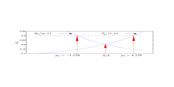
Figure 1: Illustration of the symmetric alpha divergence. Whenever $d_{p_{1}}(x,\mu)=d_{p_{2}}(\mu,x)$ (here both are 0.3) the corresponding index values sum to 3, i.e. $p_{1}+p_{2}=3$ that consequently at the point of intersection between two curves is $p_{1}=p_{2}=3/2$.

Remark 2.

Interestingly setting $p=2-q$ in PVF as ${v(\mu)}=\mu^{2-q}$ results to more commonly used form of $\alpha/\beta$-divergences in the literature [3, 22, 2]:

$$d_{\alpha}(x,\mu) ={\left(q(q-1)\right)}^{-1}\left\{x^{q}\mu^{1-q}-qx+(q-1)\mu\right\},$$ (28)

$$d_{\beta}(x,\mu) =\left(q(q-1)\right)^{-1}\left\{x^{q}-(1-q)\mu^{q}-qx\mu^{q-1}\right\}.$$ (29)

III-D Connection between Alpha and Beta Divergences

The $\beta$-divergence can be written as

$$d_{\beta}(x,\mu) ={\mu^{1-p}}\frac{x^{2-p}\mu^{p-1}-x(2-p)+\mu(1-p)}{(1-p)(2-p)},$$ (30)

where the fraction can be identified as $\alpha$-divergence. Thus the relation between two divergences is

$$d_{\beta}(x,\mu)=\mu^{1-p}d_{\alpha}(x,\mu),$$ (31)

whereas [23, 22] give other connections. Note that equality holds for either if $p=1$ or $\mu=1$

$$\mu^{1-p}=1\qquad\Rightarrow\qquad p=1\text{ or }\mu=1.$$ (32)

The solution for $p=1$, we obtain the KL divergence, the only divergence common to $\alpha/\beta$-divergences [3]. For $\mu=1$ the divergences are trivially reduced to dual cumulant

$$d_{\beta}(x,1)=d_{\alpha}(x,1)=\phi(x).$$ (33)

Here, $\mu=1$ is related to standard uniform distribution [22] with the entropy of zero that can be regarded as origin. Also note the relation [24]

$$d_{\alpha}(x,\mu)=\mu\phi(\frac{x}{\mu})=\mu d_{\beta}(\frac{x}{\mu},1).$$ (34)

Table I: Divergences, distributions and entropies indexed by $p$. The second column is ratio of $\beta$-and $\alpha$-divergences. Note also symmetry condition is $p_{1}+p_{2}=3$ for two $\alpha$-divergences.

$\mathbf{p}$	$\mathbf{\mu^{1-p}}$	Distribution	Beta	Alpha	Entropy
$0$	$\mu$	Gaussian	EU	Pearson ($\frac{1}{2}\mathcal{X}^{2}$)	L2
$1$	$1$	Poisson	KL	KL	Shannon
$\frac{3}{2}$	$\mu^{-\frac{1}{2}}$	Comp. Poisson	$-$	Hellinger dist.	$-$
$2$	$\mu^{-1}$	Gamma	IS	Reversed KL	Burg
$3$	$\mu^{-2}$	Inv. Gaussian	$-$	Rev. Pearson	$-$

The findings are summarized by Table I that presents the links between $\alpha$–type [14] and $\beta$–type divergences.

III-E Scale Transformation

Tweeide models $Tw_{p}(\mu,\varphi)$ are the only dispersion models that provide scale transformation property [5] as $\forall c\in\mathbb{R}$

$$c\;Tw_{p}(\mu,\varphi)=\;Tw_{p}(c\mu,c^{2-p}\varphi),$$ (35)

whose variance function $v(\mu)=\mu^{p}$ is scale-invariant since $v(c\mu)=c^{p}v(\mu)$. This has corresponding result in divergence side that $\alpha/\beta$-divergences are scale invariant [22, 2]

$$d_{\beta}(cx,c\mu) =c^{2-p}d_{\beta}(x,\mu),$$ (36)

$$d_{\alpha}(cx,c\mu) =cd_{\alpha}(x,\mu).$$ (37)

IV Statistical View of Beta Divergence

IV-A Density Formulation for Dispersion Models

Density of EDMs can be re-formulated based on $\beta$-divergence by using the dual form of $\beta$-divergence [4]

$$d_{\beta}(x,\mu)-\phi(x) =-x\theta+\psi(\theta)$$ (38)

that by plugging it in the EDM density, we obtain

$$p(x;\mu,\varphi) =h(x,\varphi)\exp\{\varphi^{-1}(\phi(x)-d_{\beta}(x,\mu))\}$$ (39)

$$=g(x,\varphi)\exp\{-\varphi^{-1}d_{\beta}(x,\mu)\}.$$ (40)

Here the base measures $h(\cdot,\cdot)$ and $g(\cdot,\cdot)$ are related as

$$g(x,\varphi)=h(x,\varphi)\exp\{\varphi^{-1}\phi(x)\}.$$ (41)

Example 1.

The Gaussian distribution with dispersion $\varphi=\sigma^{2}$ can be expressed as a EDM [5]

$$p(x;\mu,\sigma^{2}) =\underbrace{(2\pi\sigma^{2})^{-\frac{1}{2}}\exp\frac{-x^{2}}{2\sigma^{2}}}_{h(x,\varphi)}\exp\Big{\{}\frac{1}{\sigma^{2}}\Big{(}x\underbrace{\mu}_{\theta(\mu)}-\underbrace{\frac{\mu^{2}}{2}}_{\psi(\theta(\mu))}\Big{\}}$$

the usual form is already expressed as a $\beta$-divergence

$$p(x;\mu,\sigma^{2}) =\underbrace{(2\pi\sigma^{2})^{-\frac{1}{2}}}_{g(x,\varphi)}\exp\Big{\{}-\frac{1}{\sigma^{2}}d_{\beta}(x,\mu)\Big{\}}$$

Example 2.

For the gamma distribution with shape parameter $a$ and inverse scale parameter $b$ , the density is

$$p(x;a,b)=\frac{x^{a-1}}{\Gamma(a)}\exp\{-bx+a\log b\}$$ (42)

The mean and variance of a gamma distribution are given as $\mu=a/b$ and $Var(x)=a/b^{2}$. Hence, the dispersion becomes $\varphi=1/a$ and we have $a=1/\varphi$ and $b=1/(\mu\varphi)$. Then the density in terms of mean and dispersion parameters are given as

$$p(x;\mu,a) =\underbrace{\frac{x^{a-1}}{\Gamma(a)}a^{a}}_{h(x,\varphi)}\exp\{a(\underbrace{-\frac{1}{\mu}}_{\theta(\mu)}x-\underbrace{\log\mu)}_{\psi(\theta(\mu))}\}$$ (43)

or equivalently after adding and subtracting $\log x+1$ from the exponent we obtain

$$p(x;\mu,a) =\underbrace{\frac{x^{-1}a^{a}\exp(-a)}{\Gamma(a)}}_{g(x,\varphi)}\exp\{-ad_{\beta}(x,\mu)\}$$ (44)

Example 3.

For the Poisson distribution with dispersion $\varphi=1$, the density is given as [5]

$$p(x;\mu)=\underbrace{\frac{1}{x!}}_{h(x)}\exp\{x\underbrace{\log\mu}_{\theta(\mu)}-\underbrace{\mu}_{\psi(\theta(\mu))}\}$$ (45)

that after adding and subtracting $x\log x-x$ in the exponent we obtain equivalent beta representation of the density

$$p(x;\mu)=\underbrace{\frac{x^{x}\exp x}{x!}}_{g(x)}\exp\{-d_{\beta}(x,\mu)\}$$ (46)

This form of density formulation differs from so-called standard form of dispersion models [5] only the factor $1/2$ in the exponent, that is expressed as

$$p(x;\mu,\varphi)=g(x,\varphi)\exp\{-\frac{1}{2}\varphi^{-1}d_{\nu}(x,\mu)\},$$ (47)

where $d_{\nu}$ is unit deviance (’unit’ implies that deviance is scaled by dispersion). The deviance is a statistical term to qualify the fit of the statistics to the model [10] and is equal to $2$ times of the log-likelihood ratio of the full model to parametrized model. Log-likelihood of the full model is the maximum achievable likelihood and independent of the parameter $\mu$. Hence $\beta$-divergence is linked to the unit deviance and the log-likelihood ratio for given dispersion $\varphi$ as

$$d_{\beta}(x,\mu)=\frac{1}{2}d_{\nu}(x,\mu)=\varphi\big{\{}\mathcal{L}_{x}(x)-\mathcal{L}_{x}(\mu)\big{\}}.$$ (48)

IV-B Parameter Optimization

The last equation (48) has an immediate result for optimization of expectation parameter $\mu$ for given $p$ and $\varphi$

$$\frac{\partial d_{\beta}(x,\mu)}{\partial\mu}=-\varphi\frac{\partial\mathcal{L}_{x}(\mu)}{\partial\mu}=-\frac{(x-\mu)}{\mu^{p}}$$ (49)

that the opposite sign implies minimizing $\beta$-divergence is equal to the maximizing log-likelihood. Whereas the optimization wrt $\mu$ is trivial, the likelihood equation derived by simply plugging $\theta(\mu)$ and $\psi(\theta\mu))$ in log-density of EDM

$$\mathcal{L}_{x}(\mu,\varphi,p)=\varphi\left\{\frac{x\mu^{1-p}}{1-p}-\frac{\mu^{2-p}}{2-p}\right\}+\log h(x,\varphi,p)$$ (50)

presents difficulty for optimization of $p$ and $\varphi$ due to that the base measure $h(x,\varphi,p)$ has no closed forms except for certain values of $p$ as for $p=0,1,2,3$. For others, such as $p\in(1,2)$ for compound Poisson the function $h$ is expressed as series [5]. There are a number of approximating techniques one that saddlepoint approximation, that is interpreted as being half way between original density and Gaussian approximation as vanishing dispersion $\varphi\to 0$ [5]. Others are Fourier inversion of cumulant generating function and direct series expansion where we refer to [25] for the details.

References

- [1] D. D. Lee and H. S. Seung, “Algorithms for non-negative matrix factorization,” in Neural Information Processing Systems, vol. 13, 2001, pp. 556–562.
- [2] C. Fevotte, N. Bertin, and J. L. Durrieu, “Nonnegative matrix factorization with the itakura-saito divergence. with application to music analysis,” Neural Computation, vol. 21, 2009.
- [3] A. Cichocki, R. Zdunek, A. H. Phan, and S. Amari, Nonnegative Matrix and Tensor Factorization. Wiley, 2009.
- [4] A. Banerjee, S. Merugu, I. S. Dhillon, and J. Ghosh, “Clustering with Bregman divergences,” JMLR, vol. 6, pp. 1705–1749, 2005.
- [5] B. Jørgensen, The Theory of Dispersion Models. Chapman & Hall/CRC Monographs on Statistics & Applied Probability, 1997.
- [6] B. Jorgensen, “Exponential dispersion models,” J. of the Royal Statistical Society. Series B, vol. 49, pp. 127–162, 1987.
- [7] M. C. Tweedie, “An index which distinguishes between some important exponential families,” Statistics: applications and new directions, Indian Statist. Inst., Calcutta, pp. 579–604, 1984.
- [8] S. K. Bar-Lev and P. Enis, “Reproducibility and natural exponential families with power variance functions,” Annals of Stat., vol. 14, 1986.
- [9] M. C. Tweedie, “Functions of a statistical variate with given means, with special reference to laplacian distributions,” Proceedings of the Cambridge Philosophical Society, vol. 49, pp. 41–49, 1947.
- [10] J. A. Nelder and R. W. M. Wedderburn, “Generalized linear models,” J. of the Royal Statistical Society, Series A, vol. 135, pp. 370–384, 1972.
- [11] C. N. Morris, “Natural exponential families with quadratic variance functions,” Annals of Statistics, vol. 10, pp. 65–80, 1982.
- [12] I.Csiszar, “Eine informations theoretische ungleichung und ihre anwendung auf den beweis der ergodizitt von markoffschen ketten,” Publ. Math. Inst. Hungar. Acad., vol. 8, pp. 85–108, 1963.
- [13] J. Lafferty, “Additive models, boosting, and inference for generalized divergences,” in Proceedings of Annual Conference on Computational Learning Theory. ACM Press, 1999, pp. 125–133.
- [14] V. Kus, D. Morales, and I. Vajda, “Extensions of the parametric families of divergences used in statistical inference,” Kybernetika, vol. 44, no. 1, pp. 95–112, 2008.
- [15] M. L. Menendez, “Shannon’s entropy in exponential families: Statistical applications,” App. Mathematics Letters, vol. 13, no. 1, pp. 37–42, 2000.
- [16] P. Borwein and A. Lewis, “Moment-matching and best entropy estimation,” J of Math. Analysis and App., vol. 185, pp. 596–604, 1994.
- [17] S. Eguchi and Y. Kano, “Robustifing maximum likelihood estimation,” Institute of Statistical Mathematics in Tokyo, Tech. Rep., 2001.
- [18] M. Minami and S. Eguchi, “Robust blind source separation by beta divergence,” Neural Computation, vol. 14, pp. 1859–1886, 2002.
- [19] A. Basu, I. R. Harris, N. L. Hjort, and M. C. Jones, “Robust and efficient estimation by minimising a density power divergence,” Biometrika, vol. 85, no. 3, pp. 549–559, 1998.
- [20] M. D. Reid and R. C. Williamson, “Information, divergence and risk for binary experiments,” JMLR, vol. 12, pp. 731–817, 2011.
- [21] S. Amari, Differential-Geometrical Methods in Statistics, Editor, Ed. Springer Verlag, 1985.
- [22] A. Cichocki, S. Cruces, and S. Amari, “Generalized alpha-beta divergences and their application to robust nonnegative matrix factorization,” Entropy, vol. 13, no. 1, pp. 134–170, 2011.
- [23] A. Cichocki and S. Amari, “Families of alpha-beta-and gamma-divergences: Flexible and robust measures of similarities,” Entropy, vol. 12, pp. 1532–1568, 2010.
- [24] J. Zhang, “Divergence function, duality, and convex analysis,” Neural Computation, vol. 16, pp. 159–195, 2004.
- [25] P. K. Dunn and G. S. Smyth, “Series evaluation of tweedie exponential dispersion model densities,” Stats. & Comp., vol. 15, pp. 267–280, 2005.