Writing Reusable Digital Topology Algorithms in a Generic Image Processing Framework

Abstract

Digital Topology software should reflect the generality of the underlying mathematics: mapping the latter to the former requires genericity. By designing generic solutions, one can effectively reuse digital topology data structures and algorithms. We propose an image processing framework focused on the Generic Programming paradigm in which an algorithm on the paper can be turned into a single code, written once and usable with various input types. This approach enables users to design and implement new methods at a lower cost, try cross-domain experiments and help generalize results.

1 Introduction

Like mm (mm), dt (dt) has many applications in image analysis and processing. Both present sound mathematical foundations to handle many types of discrete images. In fact most methods from mm or dt are not tied to a specific context (image type, neighborhood, topology): they are most often described in abstract and general terms. Thus they are not limiting their field of application. However, software packages for mm and dt rarely take (enough) advantage of this generality: an algorithm is sometimes reimplemented for each image and/or each value type, or worse, written for a unique input type. Such implementations are not reusable because of their lack of genericity. These limitations often come from the implementation framework, which prohibits a generic design of algorithms. A recent and notable exception is the DGtal project, which proposes dg (dg) software tools and algorithms built in a generic # C ++ framework [1].

Thanks to the gp (gp) paradigm, provided in particular by the # C ++ language, one can design and implement generic frameworks. This paradigm is especially well-suited to the field of scientific applications where the efficiency, widespread availability and standardization of # C ++ are real assets. To this end, we have designed a paradigm dedicated to generic and efficient scientific software [2] and applied the idea of generic algorithms to mm in ip (ip) [3], as suggested by d’Ornellas and van den Boomgaard [4]. The result of our experiments is a generic library, Milena, part of the Olena image processing platform [5].

Lamy suggests to implement digital topology in ip libraries [6]. The proposed solution, applied to the ITK library [7, 8] “works for any image dimension”. In this paper, we present a framework for the generic implementation of dt methods within the Milena library, working for any image type supporting the required notions (value types, geometric and topological properties, etc.). Such a generic framework requires the definition of concepts from the domain (in particular, of an image) to organize data structures and algorithms, as explained in Sect. 2. Given these concepts it is possible to write generic algorithms, like a homotopic thinning operator making use of various definitions of the notion of simple point. We present a generic definition of such an operator in Sect. 3 and show some illustrations in Sect. 4. Section 5 concludes on the extensibility of this work along different axes: existing algorithms, new data structures and efficiency.

2 Genericity in Image Processing

In order to design a generic framework for image processing, we have previously proposed the following definition of an image [3].

Definition

An image $I$ is a function from a domain $D$ to a set of values $V$; the elements of $D$ are called the sites of $I$, while the elements of $V$ are its values.

For the sake of generality, we use the term site instead of point; e.g. a site could represent a triangle of a surface mesh used as the domain of an image. Classical site sets used as image domains encompass hyperrectangles (boxes) on regular $n$-dimensional grids, graphs and complexes (see Sect. 3).

In the gp paradigm, these essential notions (image, site set, site, value) must be translated into interfaces called concepts in Milena (Image, Site_Set, etc.) [9]. These interfaces contain the list of services provided by each type belonging to the concept, as well as its associated types. For instance, a type satisfying the Image concept must provide a domain() routine (to retrieve $D$), as well as a domain_t type (i.e. the type of $D$) satisfying the Site_Set concept. Concepts act as contracts between providers (types satisfying the concept) and users (algorithms expressing requirements on their inputs and outputs through concepts). For instance, the breadth_first_thinning routine from Algorithm 3 expects the type I (of the input image) to fulfill the requirements of the Image concept. Likewise nbh must be a Neighborhood; and is_simple and constraint must be functions taking a value of arbitrary type and returning a Boolean value (Function_v2b concept).

3 Generic Implementation of Digital Topology

Let us consider the example of homotopic skeletonization by thinning. Such an operation can be obtained by the removal of simple points (or simple sites in the Milena parlance) using Algorithm 1 [10]. A point of an object is said to be simple if its deletion does not change the topology of the object. This algorithm takes an object $X$ and a constraint $K$ (a set of points that must not be removed) and iteratively deletes simple points of $X\backslash K$ until stability is reached. Algorithm 1 is an example of an algorithm with a general definition that could be applied to many input types in theory. But in practice, software tools often allow a limited set of such input types (sometimes just a single one), because some operations (like “is simple”) are tied to the definition of the algorithm [3].

Algorithm 2 shows a more general version of Algorithm 1, where implementation-specific elements have been replaced by mutable parts: a predicate stating whether a point $p$ is simple with respect to a set $X$ (is_simple); a routine “detaching” a (simple) point $p$ from a set $X$ (detach); and a predicate declaring whether a condition (or a set of conditions) on $p$ is satisfied before considering it for removal (constraint). The algorithm takes these three functions as arguments in addition to the input $X$. Algorithm 2 is a good candidate for a generic # C ++ implementation of the breadth-first thinning strategy and has been implemented as Algorithm 3 in Milena. This algorithms implements the breadth-first traversal by using a fifo (fifo) queue. The set $X$ is represented by a binary image ($V=\{\mbox{true},\mbox{false}\}$), that must be compatible with operations performed within the algorithm. Inputs is_simple, detach and constraint have been turned into function objects (also called functors). The breadth_first_thinning routine creates and returns an image with type mln_concrete(I); it is an image type equivalent to I that allows to store data for every sites independently (which is not the case for some image types).

Algorithm 1: Breadth-First Thinning.

⬇

Data : $E$ (a set of points/sites),

$X\subseteq E$ (initial set of points),

$K\subseteq X$ (a set of points (constraint) that cannot be removed)

Result : $X$

$P$ $\leftarrow$ $\{\,p\in X\;|\;p\mbox{ is simple for }X\,\}$

while $P\neq\emptyset$ do

$S$ $\leftarrow$ $\emptyset$

for each $p\in P$ do

if $p\not\in K$ and $p\mbox{ is simple for }X$ then

$X$ $\leftarrow$ $X-\{p\}$

for each $n\,\in\,\mathcal{N}(p)\cap X$ do

$S$ $\leftarrow$ $S\cup\{n\}$

$P$ $\leftarrow$ $\emptyset$

for each $p\in S$ do

if $p\mbox{ is simple for }X$ then $P$ $\leftarrow$ $P\cup\{p\}$

Algorithm 2: A generic version of Algorithm 1.

⬇

Data : $E$, $X\subseteq E$, $\mathcal{N}$ (neighborhood),

is_simple (a function saying whether a point is simple),

detach (a routine detaching a point from $X$),

constraint (a function representing a constraint)

Result : $X$

$P$ $\leftarrow$ $\{\,p\in X\;|$ is_simple($p$, $X$) $\}$

while $P\neq\emptyset$ do

$S$ $\leftarrow$ $\emptyset$

for each $p\in P$ do

if constraint($p$) and is_simple($p$, $X$) then

$X$ $\leftarrow$ detach($X$, $p$)

for each $n\,\in\,\mathcal{N}(p)\cap X$ do

$S$ $\leftarrow$ $S\cup\{n\}$

$P$ $\leftarrow$ $\emptyset$

for each $p\in S$ do

if is_simple($p$, $X$) then $P$ $\leftarrow$ $P\cup\{p\}$

Algorithm 3: A generic # C ++ implementation of Algorithm 2 in Milena. Functors are highlighted.

⬇

template <typename I, typename N, typename F, typename G, typename H>

mln_concrete(I)

breadth_first_thinning(const Image<I>& input_,

const Neighborhood<N>& nbh_,

Function_v2b<F>& is_simple_,

G& detach,

const Function_v2b<H>& constraint_)

{

//Convert arguments to their exact types and initialize ‘output’.

const I& input = exact(input_);

const N& nbh = exact(nbh_);

F& is_simple = exact(is_simple_);

const H& constraint = exact(constraint_);

mln_concrete(I) output = duplicate(input);

is_simple.set_image(output); //Bind ‘output’ to ‘is_simple’.

detach.set_image(output); //Bind ‘output’ to ‘detach’.

//Step #1. Initialize a FIFO queue with simple points candidates.

typedef mln_psite(I) psite;

p_queue_fast<psite> queue;

//Image ‘in_queue’ records whether a point site is in the queue.

mln_ch_value(I, bool) in_queue;

initialize(in_queue, input);

data::fill(in_queue, false);

mln_piter(I) p(output.domain());

for_all(p) //$\forall$ ‘p’ $\in$ the domain of ‘output’…

if (output(p) && constraint(p) && is_simple(p)) {

queue.push(p); in_queue(p) = true; //Push ‘p’ into the queue.

}

//Step #2. Process the FIFO queue until it is empty.

while (!queue.is_empty()) {

psite p = queue.pop_front(); in_queue(p) = false;

if (output(p) && constraint(p) && is_simple(p)) {

detach(p); //‘p’ is simple and passes the constraint; detach it.

//Process the neighbors of ‘p’.

mln_niter(N) n(nbh, p);

for_all(n) //$\forall$ ‘n’ in the neighborhood of ‘p’…

if (output.domain().has(n) //Prevent out-of-bound accesses.

&& output(n) && constraint(n) && is_simple(n)

&& !in_queue(n)) {

queue.push(n); in_queue(n) = true; //Push ‘n’ into the queue.

}

}

}

return output;

}

Simple Point Characterization Implementation

There are local characterizations of simple points in 2D, 3D and 4D, which can lead to lut (lut) based implementations [11]. However, since the number of configurations of simple and non-simple points in $\mathbb{Z}^{d}$ is $2^{3^{d}-1}$, this approach can only be used in practice in 2D (256 configurations, requiring a lut of 32 bytes) and possibly in 3D (67,108,864 configurations, requiring a lut of 8 megabytes). The 4D case exhibits $2^{80}$ configurations, which is intractable using a lut, as it would need 128 zettabytes (128 billions of terabytes) of memory. Couprie and Bertrand have proposed a more general framework for checking for simple points using cell complexes [11] and the collapse operation. Intuitively, complexes can be seen as a generalization of graphs. An informal definition of a simplicial complex (or simplicial $d$-complex) is “a set of simplices” (plural of simplex), where a simplex or $n$-simplex is the simplest manifold that can be created using $n$ points (with $0\leq n\leq d$). A 0-simplex is a point, a 1-simplex a line segment, a 2-simplex a triangle, a 3-simplex a tetrahedron. A graph is indeed a 1-complex. Figure 1(a) shows an example of a simplicial complex. Likewise, a cubical complex or cubical $d$-complex can be thought as a set of $n$-faces (with $0\leq n\leq d$) in $\mathbb{Z}^{d}$, like points (0-faces), edges (1-faces), squares (2-faces), cubes (3-faces) or hypercubes (4-faces). Figure 1(b) depicts a cubical complex sample.

Complexes support a topology-preserving transformation called collapse. An elementary collapse removes a free pair of faces of a complex, like the square face $f_{1}$ and its top edge $e_{1}$, or the edge $e_{2}$ and its top vertex $v$, in Fig. 1(b). The pair $(f_{2},e_{3})$ cannot be removed, since $e_{3}$ also belongs to $f_{3}$. Successive elementary collapses form a collapse sequence that can be used to remove simple points. Collapse-based implementations of simple-point deletion can always be used in 2D, 3D and 4D, though they are less efficient than their lut-based counterparts. On the other hand, they provide some genericity as the collapse operation can have a single generic implementation on complexes regardless of their structure.

(a) A simplicial 3-complex, composed of 0-faces (vertices), 1-faces (edges), 2-faces (triangles) and a 3-face (tetrahedron).

(b) A cubical 2-complex, composed of 0-faces (vertices), 1-faces (edges) and 2-faces (squares).

Figure 1: Examples of cell complexes.

4 Illustrations

Using this generic approach, Algorithm 3 can be used to compute skeletons of various input images.

4.1 Skeleton of a 2D Binary Image

(a) 2D binary image.

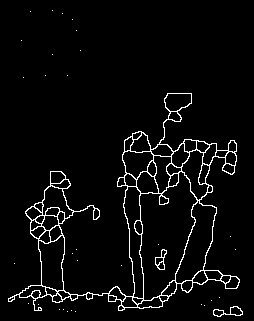
(b) Skeleton of 2(a) with no constraint

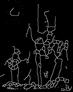
(c) Skeleton of 2(a) where end points of the initial image have been preserved.

Figure 2: Computation of skeletons from a 2D binary regular image.

Our first illustration uses a classical 2D binary image built on a square grid (Fig. 2(a)). The following lines produces the result shown on Fig. 2(b).

⬇

typedef image2d<bool> I;

typedef neighb2d N;

I output =

breadth_first_thinning(input,

c4(),

is_simple_point2d<I, N>(c4(), c8()),

detach_point<I>(),

no_constraint());

I and N are introduced as aliases of the image and neighborhood types for convenience. The breadth_first_thinning algorithm is called with five arguments, as expected. The first two ones are the input image and the (4-connectivity) neighborhood used in the algorithm. The last three ones are the functors governing the behavior of the thinning operator. The call is_simple_point2d<I, N>(c4(), c8()) creates a simple point predicate based on the computation of the 2D connectivity numbers [10] associated with the 4-connectivity for the foreground and the 8-connectivity for the background. To compute these numbers efficiently, is_simple_point2d uses a lut containing all the possible configurations in the 8-connectivity neighborhood of a pixel. detach_point<I> is a simple functor removing a pixel by giving it the value “false”. Finally, no_constraint is an empty functor representing a lack of constraint.

We also present a variation of the previous example where the fifth argument passed to the function is an actual constraint, preserving all end points of the initial image (see Fig. 2(c)). This result is obtained by invoking the generic functor is_not_end_point in the following lines. This call creates a predicate characterizing end points by counting their number of neighbors.

⬇

I output_with_end_points =

breadth_first_thinning(input,

c4(),

is_simple_point2d<I, N>(c4(), c8()),

detach_point<I>(),

is_not_end_point<I, N>(c4(), input));

4.2 Skeleton of a 3D Binary Image

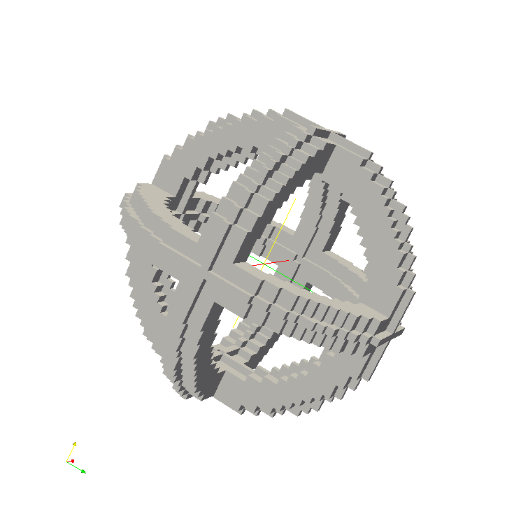
(a) 3D binary image.

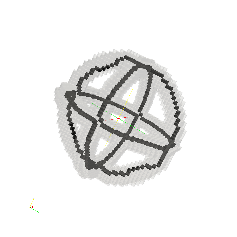
(b) Skeleton (dark voxels) of 2(a) with no constraint superimposed on the initial image (light voxels).

Figure 3: Computation of the skeleton of 3D binary regular image.

This second example in 3D is similar to the previous one in 2D. The domain of the image is a box on a cubical grid; the 26- and the 6-connectivity are respectively used for the foreground and the background. The output of Fig. 3(b) is obtained from the 3D volume shown in Fig. 3(a) with the following lines.

⬇

typedef image3d<bool> I;

typedef neighb3d N;

I output =

breadth_first_thinning(input,

c26(),

is_simple_point3d<I, N>(c26(), c6()),

detach_point<I>(),

no_constraint());

The only real difference with the previous example is the use of the functor is_simple_point3d. The default implementation of this predicate uses an on-the-fly computation of 3D connectivity numbers. We have also implemented a version based on a precomputed lut which showed significant speed-up improvements.

Please note that the predicates is_simple_point2d and is_simple_point3d are specifically defined for a given topology in order to preserve performances.

4.3 Thick Skeleton of a 3D Mesh Surface

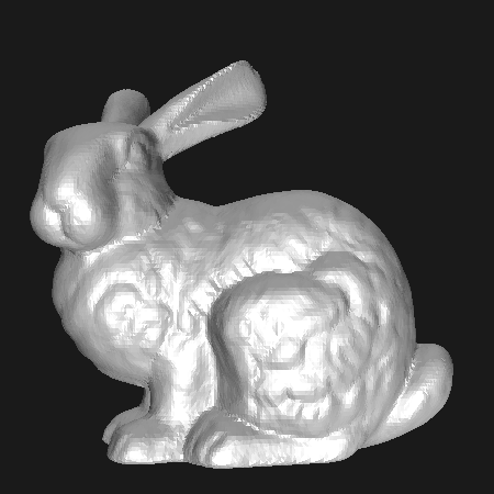
(a) Triangle mesh surface.

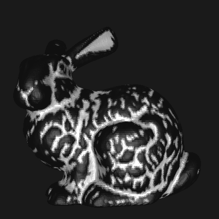
(b) Surface curvature.

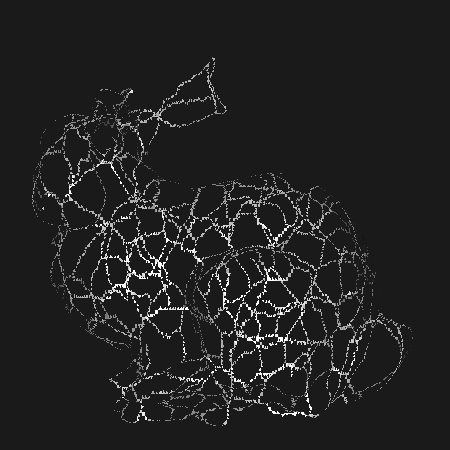
(c) Surface skeleton.

Figure 4: Computation of a skeleton using breadth-first thinning. The triangle mesh surface 4(a) (35,286 vertices and 70,568 triangles) is seen as a simplicial 2-complex. The image of curvature 4(b) is computed on the edges of the mesh, and simplified using an area opening filter. All curvature regional minima are then removed from the mesh, and the skeleton 4(c) is obtained with Algorithm 3 using the collapse operation.

In this third example, we manipulate discrete mesh surfaces composed of triangles. The input of the thinning operator is a surface containing “holes”, obtained from the mesh shown in Fig. 4(a) by removing triangles located in regional minima of the surface’s curvature (darkest areas of Fig. 4(b)). The result presented in Fig. 4(c) is obtained with the following lines. Types are not shown to make this code more readable.

⬇

output = breadth_first_thinning(input,

nbh,

is_simple_triangle,

detach_triangle,

no_constraint());

In the previous code, input is a triangle-mesh surface represented by an image built on a simplicial 2-complex and nbh represents an adjacency relationship between triangles sharing a common edge. Function objects is_simple_triangle and detach_triangle are operations compatible with input’s type; they are generic routines based on the collapse operation mentioned in Sect. 3, working with any complex-based binary image.

The input image is constructed so that the sites browsed by the for_all loops in Algorithm 3 are only 2-faces (triangles), while preserving access to values at 1-faces and 0-faces. Thus, even though they receive 2-faces as input parameters, is_simple_triangle and detach_triangle are able to inspect the adjacent 1-faces and 0-faces and determine whether and how a triangle can be completely detached from the surface through a collapse sequence.

The resulting skeleton is said to be thick, since it is composed of triangles connected by a common edge. The corresponding complex is said to be pure, as it does not contain isolated 1-faces or 0-faces (that are not part of a 2-face).

4.4 Thin Skeleton of a 3D Mesh Surface

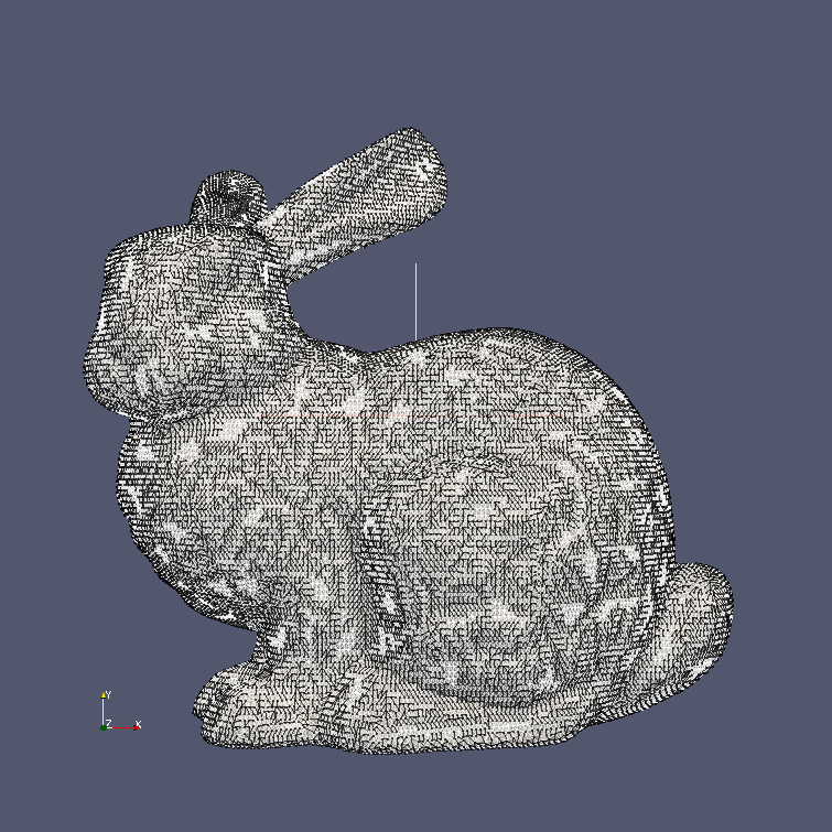
(a) Ultimate 2-collapse of Fig. 4(a).

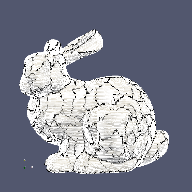
(b) Ultimate 1-collapse of 5(a)

Figure 5: Thin skeleton obtain by 2- and 1-collapse.

To obtain a thin skeleton, we can use a strategy based on successive $n$-collapse operations, with $n$ decreasing [12]. From the input of the previous example, we can obtain a ultimate 2-collapse by removing all simple pairs composed of a 2-face and a 1-face (a triangle and an adjacent edge). The following lines compute such an ultimate 2-collapse. The iteration on input’s domain is still limited to triangles (2-faces).

⬇

collapse2 = breadth_first_thinning(input,

nbh,

is_triangle_in_simple_pair,

detach_triangle_in_simple_pair,

no_constraint());

Functor is_triangle_in_simple_pair checks whether a given triangle is part of a simple pair, and if so detach_triangle_in_simple_pair is used to remove the pair. Thinning the initial surface with this “simple site” definition produces a mesh free of 2-faces (triangles), as shown in Fig. 5(a).

From this first skeleton, we can compute an ultimate 1-collapse, by removing all simple pairs composed of an edge (1-face) and a vertex (0-face). This skeleton is produced with the following code, where input2 is an image created from collapse2, and for which the domain of has been set to the edges of the complex, (instead of the triangles).

⬇

collapse1 = breadth_first_thinning(input2,

nbh,

is_edge_in_simple_pair,

detach_edge_in_simple_pair,

no_constraint());

Here is_edge_in_simple_pair and detach_edge_in_simple_pair respectively test and remove an edge along with a vertex that form a simple pair. The result is a simplified skeleton, with no isolated branches, as the lack of constraint (no_constraint) does not preserve them. The output of the ultimate 1-collapse on the bunny mesh is depicted in Fig. 5(b). It contains the crest lines that form the boundaries of catchment basins, such as in the watershed transform, and, in addition, the crest lines that make the previous ones connect one to another.

Note that in both cases, the neighborhood object nbh is the same, as it represents the adjacency of two $n$-faces connected by a common adjacent $(n-1)$-face. In the case of the 2-collapse, the neighborhood of a site (triangle) is the set of adjacent triangles connected by an edge, while in the case of the 1-collapse, the neighborhood of a site (edge) is the set of adjacent edges connected by a vertex.

4.5 Execution Times

Table 1 shows the execution times of the previous illustrations, computed on a PC running Debian GNU/Linux 6.0.4, featuring an Intel Pentium 4 CPU running at 3.4 GHz with 2 GB RAM at 400 MHz, using the # C ++ compiler g++ (GCC) version 4.4.5, invoked with optimization option ‘-03’. The first three test cases use a simple point criterion based on connectivity numbers, while the last three use a collapse-based definition.

Table 1: Execution times of Algorithm 3 for various inputs. Figures correspond to the time spent in the breadth_first_thinning routine only.

Input	Input size	Constraint	Output	Time
2D image (Fig. 2(a))	321 $\times$ 254 pixels	None	Fig. 2(b)	0.08 s
2D image (Fig. 2(a))		End points	Fig. 2(c)	0.10 s
3D image (Fig. 3(a))	41 $\times$ 41 $\times$ 41 voxels	None	Fig. 3(b)	2.67 s
Mesh (2-faces only) (Fig. 4(a))		None	Fig. 4(c)	159.53 s
Mesh (2- and 1-faces)	35,286 0-faces +	None	Fig. 5(a)	68.78 s
(Fig. 4(a))	105,852 1-faces +		(2-collapse)
Mesh (1- and 0-faces)	70,568 2-faces	None	Fig. 5(b)	46.18 s
(Fig. 5(a))			(1-collapse)

5 Conclusion

We have presented building blocks to implement reusable dt algorithms in an ip framework, Milena. Given a set of theoretical constraints on its inputs, an algorithm can be written once and reused with many compatible image types. This design has previously been proposed for mm, and can be applied to virtually any image processing field. Milena is Free Software released under the gpl, and can be freely downloaded from http://olena.lrde.epita.fr/.

A strength of generic designs is their ability to extend and scale easily and efficiently. First, generic algorithms are extensible because of their parameterization. For instance, the behavior of Algorithm 3 can be changed by acting on the simple point definition or the set of constraints. The scope of this algorithm, initially designed to produce homotopic thinnings of binary skeleton, can even be extended further to handle gray-level images and produce gray-level thinnings. From a theoretical point of view, gray-level images can be processed by decomposing them into different sections. The equivalent of detaching a simple point in a binary image is the lowering of a destructible point in a gray-level context [13]. We have been able to produce gray-level skeletons with Algorithm 3 by simply replacing the is_simple and detach operations by is_destructible and lower functors (see Fig. 6). In the case of a 2D regular images on a square grid, this operation is straightforward as a destructible point can also be characterized locally using new definitions of connectivity numbers.

Generic algorithms can thereafter be turned into patterns or canvases [14] allowing the implementation of many algorithms sharing a common core. For example Milena implements morphological algorithms like dilation and erosion, reconstructions, etc. depending on the browsing strategy. dt could also benefit from a canvas-based approach. The framework can also be extended with respect to data structures. Milena provides site sets based on boxes, graphs and complexes, but more can be added to the library (e.g. combinatorial maps, orders, etc.) and benefit from existing algorithms and tools.

Finally, our approach can take advantage of properties of input types (regularity of the site set, isotropic adjacency relationship, etc.) and allow users to write specialized versions of their algorithms for such subsets of data types, leading to faster or less memory-consuming implementations [15].

5.0.1 Acknowledgments

The authors thank Jacques-Olivier Lachaud, who reviewed this paper, for his valuable comments, as well the initial reviewers from the WADGMM workshop.

This work has been conducted in the context of the SCRIBO project (http://www.scribo.ws/) of the Free Software Thematic Group, part of the “System@tic Paris-Région” Cluster (France). This project is partially funded by the French Government, its economic development agencies, and by the Paris-Région institutions.

(a) 2D gray-level image.

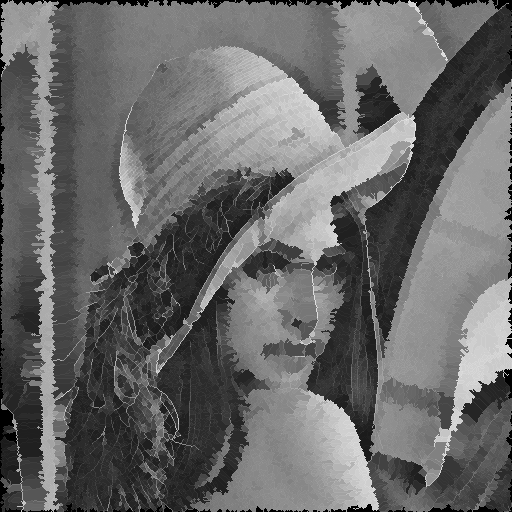
(b) Gray-level skeleton.

Figure 6: Computation of a gray-level skeleton.

References

- [1] DGtal: Digital geometry tools and algorithms. http://liris.cnrs.fr/dgtal/
- [2] Géraud, Th., Levillain, R.: Semantics-driven genericity: A sequel to the static C++ object-oriented programming paradigm (SCOOP 2). In: Proceedings of the 6th International Workshop on Multiparadigm Programming with Object-Oriented Languages (MPOOL), Paphos, Cyprus (July 2008)
- [3] Levillain, R., Géraud, Th., Najman, L.: Milena: Write generic morphological algorithms once, run on many kinds of images. In Wilkinson, M.H.F., Roerdink, J.B.T.M., eds.: Mathematical Morphology and Its Application to Signal and Image Processing – Proceedings of the Ninth International Symposium on Mathematical Morphology (ISMM). Volume 5720 of Lecture Notes in Computer Science., Groningen, The Netherlands, Springer Berlin / Heidelberg (August 2009) 295–306
- [4] d’Ornellas, M.C., van den Boomgaard, R.: The state of art and future development of morphological software towards generic algorithms. International Journal of Pattern Recognition and Artificial Intelligence 17(2) (March 2003) 231—255
- [5] EPITA Research and Developpement Laboratory (LRDE): The Olena image processing platform. http://olena.lrde.epita.fr
- [6] Lamy, J.: Integrating digital topology in image-processing libraries. Computer Methods and Programs in Biomedicine 85(1) (2007) 51–58
- [7] Ibáñez, L., Schroeder, W., Ng, L., Cates, J., the Insight Software Consortium: The ITK Software Guide. second edn. Kitware, Inc. (November 2005)
- [8] National Library of Medicine: Insight segmentation and registration toolkit (ITK). http://www.itk.org/
- [9] Levillain, R., Géraud, Th., Najman, L.: Why and how to design a generic and efficient image processing framework: The case of the Milena library. In: Proceedings of the IEEE International Conference on Image Processing (ICIP), Hong Kong (September 2010) 1941–1944
- [10] Bertrand, G., Couprie, M.: Transformations topologiques discrètes. In Coeurjolly, D., Montanvert, A., Chassery, J.M., eds.: Géométrie discrète et images numériques. Hermes Sciences Publications (2007) 187–209
- [11] Couprie, M., Bertrand, G.: New characterizations of simple points in 2D, 3D, and 4D discrete spaces. IEEE Transactions on Pattern Analysis and Machine Intelligence 31(4) (April 2009) 637–648
- [12] Cousty, J., Bertrand, G., Couprie, M., Najman, L.: Collapses and watersheds in pseudomanifolds. In: Proceedings of the 13th International Workshop on Combinatorial Image Analysis (IWCIA), Springer-Verlag (2009) 397–410
- [13] Couprie, M., Bezerra, F.N., Bertrand, G.: Topological operators for grayscale image processing. Journal of Electronic Imaging 10(4) (2001) 1003–1015
- [14] d’Ornellas, M.C.: Algorithmic Patterns for Morphological Image Processing. PhD thesis, Universiteit van Amsterdam (2001)
- [15] Levillain, R., Géraud, Th., Najman, L.: Une approche générique du logiciel pour le traitement d’images préservant les performances. In: Proceedings of the 23rd Symposium on Signal and Image Processing (GRETSI), Bordeaux, France (September 2011) In French.