Semi-classical approximation for the second harmonic generation in nanoparticles

Abstract

Second harmonic generation by spherical nanoparticles is a non-local optical process that can also be viewed as the result of the non-linear response of the thin interface layer. The classical electrodynamic description, based e.g. on the non-linear Mie theory, entails the knowledge of the dielectric function and the surface non-linear optical susceptibility, both quantities are usually assumed to be predetermined, for instance from experiment. We propose here an approach based on the semi-classical approximation for the quantum sum-over-states expression that allows to capture the second-order optical process from first principles. A key input is the electronic density, which can be obtained from effective single particle approaches such as the density-functional theory in the local density implementation. We show that the resulting integral equations can be solved very efficiently rendering thus the treatment of macroscopic systems. As an illustration we present numerical results for the magic Na${}_{2869}^{-}$ cluster.

I Introduction

For the description of a wide range of phenomena in physics and chemistry one is faced with the question of how to predict in a reliable and system specific way the response to external electromagnetic fields that impart energy $\omega$ and possibly momentum $\mathbf{k}$ to the system Mahan (2000). To name but few examples, we mention here the response of nanoparticles to light in the linear Halas et al. (2011) and the non-linear regimes Roke (2009). For electrons as a perturbation we refer to the overview  García de Abajo (2010). A well-studied route to address these issues is the concept of the dielectric response functions which is detailed in standard books such as in  Mahan (2000), but also in recent reviews, e.g. in Refs.  Halas et al. (2011); Roke (2009); García de Abajo (2010).

For extended bulk metals and metallic surfaces the dielectric response was extensively studied (Ref. Liebsch (1997); Andersen and Hübner (2002) and references therein). An extension to finite-size systems brings about a number of new aspects that complicate the theory but at the same time offer new opportunities for the occurrence of new phenomena. For example, it is known that the second harmonic generation (SHG) is forbidden in systems with an inversion symmetry on the dipole approximation level. Therefore Östling, Stampfli, and Bennemann Östling et al. (1993) and Dewitz, Hübner, and Bennemann Dewitz et al. (1996) proposed the anharmonic oscillator model to describe the second-order non-linear response from spherical systems. A further step was undertaken by Dadap et al. Dadap et al. (1999) who considered the small-particle limit ($ka<1$) and described SHG as a mixture of dipole and quadrupole excitation processes ($a$ stands for the system size). It was also shown how to connect the model output to experimentally observed quantities, i.e. the elements of the non-linear optical susceptibility tensor $\chi^{(2)}(\omega)$. In this approach the inversion symmetry is not a necessary assumption as it is assumed that the second harmonic generation originates from the thin surface layer, where the symmetry is broken anyway. This idea can be extended in several directions as was demonstrated in numerous works: Pavlyukh and Hübner Pavlyukh and Hübner (2004) developed the non-linear Mie theory valid for particles of arbitrary sizes, de Beer and Roke included the sum-frequency generation mechanism into the considerations de Beer and Roke (2009), the cylindrical geometry was treated by Dadap Dadap (2008) and finally the theory for arbitrarily shaped particles was developed by de Beer, Roke, and Dadap de Beer et al. (2011).

All these theories based on classical electrodynamics rely on the knowledge of the frequency-dependent dielectric function and the non-linear optical susceptibility tensor. With the fabrication processes being perfected and the system sizes tending smaller and smaller one may wonder to which extent quantum effects are important and whether it is justified to use the same susceptibility tensor to describe semi-infinite and finite size systems on the nanometer range. To shed light on these issues, it is desirable to have a quantum theory for the non-linear response on the nanoscale. The fully atomistic approach seems to be out of reach for present computers, as currently maximally hundreds of atoms are possible to treat using quantum chemistry codes. Yet, the outstanding question is, how important are the electronic correlation effects and is there possibly a way to stay on the solid quantum theory basis while treating larger systems?

There is an affirmative answer to these questions as was demonstrated recently in the linear optics case by Prodan and Nordlander Prodan and Nordlander (2003). They succeeded to push the limits of the time-dependent density functional theory (TDDFT) to metallic systems containing millions of atoms. But at the same time they demonstrated that for these system sizes the semi-classical approach becomes very accurate. This is a marked finding as it allows to replace the complicated sum-over-states quantum mechanical expression Orr and Ward (1971) for the polarizability tensor with a single integral equation. Consequently, there is only one parameter in the theory: the ionic density distribution. With some reasonable assumptions about the ionic density such as in the jellium model (this assumption is reasonable even for molecular structures, as we have shown recently Pavlyukh and Berakdar (2009, 2010) for fullerenes. The usefulness of the jellium model was demonstrated by the pioneering works of Ekardt on sodium clusters Ekardt (1984, 1985) or of Puska and Nieminen on C₆₀ Puska and Nieminen (1993).) we can obtain the ground state electronic density from the solution of the Kohn-Sham equations and express the response function in its terms. The Drude dielectric function follows automatically.

The semi-classical approximation is rooted in the work of Mukhopadhyay and Lundqvist Mukhopadhyay and Lundqvist (1975) who derived the corresponding integral equation within linear response theory. Their theory was applied in numerous cases ranging from plasmons in the jellium model to collective resonances in C₆₀ Vasvári (1996) or carbon nanotubes Vasvári (1997). The equation can also be derived starting from the quantum mechanical sum-over-states expressions Pavlyukh et al. (2012) and using the assumption that the frequency of the external field is large compared with the single-particle gap ($\omega\gg E_{g}$) Ichikawa (2011).

One may wonder why this program was not implemented for nonlinear optical processes. As a matter of the fact, already in 1973 Wang, Chen and Bower Wang et al. (1973) classically treated second harmonic generation from alkali metals. A decade later Apell Apell (1983) derived an expression for the second harmonic current in the form:

$$\mathbf{j}(\mathbf{r},2\omega)=\upalpha\big{[}f(\mathbf{E}\cdot\mathbf{\nabla})\mathbf{E}+\upbeta(\mathbf{\nabla}f)E^{2}+\upgamma f(\mathbf{\nabla}\cdot\mathbf{E})\mathbf{E}\big{]},$$ (1)

where for the unperturbed ground state electron density in the form $n(\mathbf{r})=n_{0}f(\mathbf{r})$ the $\upalpha$ parameter is a function of $n_{0}$ and $\omega$, whereas $\upbeta$ and $\upgamma$ are constants. The theory gained less attention than, for example, the Mukhopadhyay and Lundqvist work because the connection to quantum mechanics was lost. Here we mention nonetheless numerous works in the field extending over more than three decades: the small homogeneous spherical particle limit Hua and Gersten (1986), the Rayleigh-Gans scattering approximation for a lattice of such particles Martorell et al. (1997), second harmonic generation by two-dimensional particles Valencia et al. (2003), or a more recent treatment of arbitrary geometries Zeng et al. (2009). Notice that the assumption of homogeneous electron density distribution within the sample is an inevitable component of such classical theories.

It is possible to revive the theory by noting that the electric field ($\mathbf{E}$) in Eq. (1) must also include the induced field. This simple observation immediately raises the level of the theory to the random phase approximation (RPA) or, if we include electronic correlations, to TDDFT level. Our manuscript is, hence, a formalization of this message.

To this end we first derive an expression analogous to (1) starting from the sum-over-state quantum mechanical formula for the non-linear optical susceptibility Orr and Ward (1971) and employing the high-frequency approximation. Although quite technical, we believe that this derivation (Appendix A) has its own merits as it establishes the equivalence of the hydrodynamic approximation of Apell and the high-frequency semi-classical expansion. It is interesting to notice that the $1/\omega^{4}$ asymptotic behavior of this quantity is at variance with the results of Scandolo and Bassani Scandolo and Bassani (1995) who predict a $1/\omega^{6}$ decay. This seems, however, to be a direct consequence of the assumption of the all-dipole excitation mechanism that underly their study. It is possible to prove from general principles that the inclusion of the quadrupole excitations leads to the $1/\omega^{4}$ asymptotics Satitkovitchai (2009).

Our derivation raises the question of whether it is sufficient to know the unperturbed ground state density to obtain the lowest order approximation for an arbitrary response function. We recall that from the point of view of the diagrammatic perturbation theory Ward (1965) SHG comprises three processes in which the $2\omega$ photon is emitted before, between or after the absorption of two $\omega$-photons. Consequently, one might wonder if each diagram of this expansion can also be expressed in terms of $n(\mathbf{r})$. As we demonstrate below, the answer is negative, one additionally needs the one-particle density matrix $\gamma(\mathbf{r},\mathbf{r}^{\prime})$ whose diagonal elements are given by $n(\mathbf{r})$. This comes not as a surprise if we consider the analogy with the orbital-free kinetic density functional theory Wang and Carter (2002) where this matrix enters the kinetic energy term.

The non-linear susceptibility relates the second-order induced density to the local electric field. The latter is a microscopic quantity that can be connected to the external field by knowing the linear response function. In the linear case it is a standard route to get the RPA dielectric response. In the non-linear case the procedure is, probably, less known. Therefore, we follow here a very pedagogical treatment of Liebsch and Schaich Liebsch and Schaich (1989). In fact, they applied a trick suggested by Zangwill and Soven Zangwill and Soven (1980) to avoid the summation over the infinite number of unoccupied states for the calculation of the response functions. This allowed them to describe SHG at simple metal surfaces as effectively one dimensional systems (it is basically the same approach that enabled Prodan and Nordlander Prodan and Nordlander (2003) to treat very large spherical systems).

The outline of this work is as follows: In Sec. II we start with the most general relation between the induced densities and the effective fields [Eq. (2.5) of Liebsch and Schaich, Phys. Rev. B 40, 5401 (1989)] and formulate integral equations for the induced density with the non-interacting response functions as kernels. In Sec. III we discuss the case of a spherical symmetry and the simplifications it implies for the numerics. Finally, the second harmonic response of the magic Na${}_{2869}^{-}$ cluster is presented in Sec. IV for the illustration of our theory. Based on our recently developed method for the solution of integral equations of this type we are able to drastically reduce the computational cost from $\mathcal{O}(N^{3})$ to $\mathcal{O}(N)$, where $N$ is the number of mesh points to represent the density.

We use atomic units, i. e., $\hbar=e=m_{e}=4\pi\varepsilon_{0}=1$ throughout. Two appendices contain mathematical details to make the exposition in Secs. II-IV self-contained.

II Integral equations

Our theory can easily be extended to include electron correlation effects by using the exchange correlation functional of DFT. Our formulation here is at the random phase approximation level. Within this approximation the density-density response function can be obtained as

$$\chi(\mathbf{r},\mathbf{r}^{\prime};\omega)=\chi^{(0)}(\mathbf{r},\mathbf{r}^{\prime};\omega)+\int d\mathbf{r}_{1}\!\!\int d\mathbf{r}_{2}\,\chi^{(0)}(\mathbf{r},\mathbf{r}_{1};\omega)\\ \times v(\mathbf{r}_{1}-\mathbf{r}_{2})\,\chi(\mathbf{r}_{2},\mathbf{r}^{\prime};\omega),$$ (2)

where $v(\mathbf{r}-\mathbf{r}_{1})$ is the Coulomb potential and $\chi^{(0)}(\mathbf{r},\mathbf{r}^{\prime};\omega)$ is the non-interacting density-density response function (known as Lindhard function for the homogeneous electron gas in three dimensions, 3D):

$$\begin{split}\chi^{(0)}(\mathbf{r},\mathbf{r}^{\prime};\omega)=2\sum_{i,j}&\frac{f_{i}-f_{j}}{\omega+E_{i}-E_{j}+i\eta}\\ &\quad\times\psi_{i}(\mathbf{r})\psi_{j}^{*}(\mathbf{r})\psi_{j}(\mathbf{r}^{\prime})\psi_{i}^{*}(\mathbf{r}^{\prime}),\end{split}$$ (3)

where $f$ is the Fermi function and $i$, $j$ refer to the collections of quantum numbers that uniquely characterize the electronic states of the system. The infinitesimally small positive number $\eta$ shifts the poles from the real axis and ensures, thus, the causality of the response function. In what follows we will assume it can be incorporated in the $\omega$ variable.

Let us consider the response of the system subject to the harmonic electric field oscillating at the frequency $\omega$, i.e. $\varphi^{(0)}(\mathbf{r};t)=\varphi^{(0)}(\mathbf{r})\,e^{-i\omega t}$. Then, the induced density which oscillates at the frequency of the applied field is given by:

$$\delta n^{(1)}(\mathbf{r})=\int\!d\mathbf{r}^{\prime}\chi(\mathbf{r},\mathbf{r}^{\prime};\omega)\,\varphi^{0}(\mathbf{r}^{\prime})\\ =\int\!\!d\mathbf{r}^{\prime}\chi^{(0)}(\mathbf{r},\mathbf{r}^{\prime};\omega)\,\varphi^{(1)}(\mathbf{r}^{\prime}),$$ (4)

where $\varphi^{(1)}(\mathbf{r})$ is the induced local field oscillating at the fundamental frequency and consisting of the external potential plus the Hartree potential corresponding to the induced density:

$$\varphi^{(1)}(\mathbf{r})=\varphi^{(0)}(\mathbf{r})+\int\!\!d\mathbf{r}^{\prime}v(\mathbf{r}-\mathbf{r}^{\prime})\,\delta n^{(1)}(\mathbf{r}^{\prime}).$$ (5)

The induced density oscillating at the double frequency results from the non-linear process described by the $\chi^{(0)}_{2}$ response function and from the linear response to the local field $\varphi^{(2)}(\mathbf{r})$ oscillating at $2\omega$:

$$\delta n^{(2)}(\mathbf{r})=\int\!\!d\mathbf{r}^{\prime}\!\int\!\!d\mathbf{r}^{\prime\prime}\chi^{(0)}_{2}(\mathbf{r};\mathbf{r}^{\prime},\mathbf{r}^{\prime\prime};\omega)\,\varphi^{(1)}(\mathbf{r}^{\prime})\,\varphi^{(1)}(\mathbf{r}^{\prime\prime})\\ +\int d\mathbf{r}^{\prime}\chi^{(0)}(\mathbf{r},\mathbf{r}^{\prime};\omega)\,\varphi^{(2)}(\mathbf{r}^{\prime}).$$ (6)

Because there is no external field at $2\omega$ the local field at this frequency is given by the Hartree potential:

$$\varphi^{(2)}(\mathbf{r})=\int\!\!d\mathbf{r}^{\prime}v(\mathbf{r}-\mathbf{r}^{\prime})\,\delta n^{(2)}(\mathbf{r}^{\prime}).$$ (7)

Equations 4 and 5 yield the integral equation for the linear density:

$$\delta n^{(1)}(\mathbf{r})=\xi^{(1)}(\mathbf{r})+\\ \int\!\!d\mathbf{r}^{\prime}\!\int\!\!d\mathbf{r}^{\prime\prime}\,\chi^{(0)}(\mathbf{r},\mathbf{r}^{\prime};\omega)\,v(\mathbf{r}^{\prime}-\mathbf{r}^{\prime\prime})\,\delta n^{(1)}(\mathbf{r}^{\prime\prime}),$$ (8)

while eqs. 6 and 7 result in the integral equation for the second harmonic density:

$$\delta n^{(2)}(\mathbf{r})=\xi^{(2)}(\mathbf{r})+\\ \int\!\!d\mathbf{r}^{\prime}\!\int\!\!d\mathbf{r}^{\prime\prime}\,\chi^{(0)}(\mathbf{r},\mathbf{r}^{\prime};\omega)\,v(\mathbf{r}^{\prime}-\mathbf{r}^{\prime\prime})\,\delta n^{(2)}(\mathbf{r}^{\prime\prime}).$$ (9)

We defined the source terms following Liebsch and Schaich (1989) as:

$$\xi^{(1)}(\mathbf{r}) = \int\!\!d\mathbf{r}^{\prime}\chi^{(0)}(\mathbf{r},\mathbf{r}^{\prime};\omega)\,\varphi^{(0)}(\mathbf{r}^{\prime}),$$ (10)

$$\xi^{(2)}(\mathbf{r}) = \int\!\!d\mathbf{r}^{\prime}\!\int\!\!d\mathbf{r}^{\prime\prime}\chi^{(0)}_{2}(\mathbf{r};\mathbf{r}^{\prime},\mathbf{r}^{\prime\prime};\omega)\,\varphi^{(1)}(\mathbf{r}^{\prime})\,\varphi^{(1)}(\mathbf{r}^{\prime\prime}).$$ (11)

Eqs. (8, 10) and eqs. (9, 11) when coupled with an appropriate approximation for the non-interacting response functions allow to completely describe the linear and the second-harmonic response.

The semi-classical approximation for the $\xi^{(1)}(\mathbf{r})$ has already been derived previously Pavlyukh et al. (2012) with the result:

$$\xi^{(1)}(\mathbf{r})=\frac{1}{\omega^{2}}\Big{(}\mathbf{\nabla}n(\mathbf{r})\cdot\mathbf{\nabla}\varphi^{(0)}(\mathbf{r})-n(\mathbf{r})\Delta\varphi^{(0)}(\mathbf{r})\Big{)}.$$ (12)

In Appendix A we derive the second-harmonic generation source term (49) that can be represented as:

$$\xi^{(2)}(\mathbf{r})=\frac{1}{2\omega^{4}}\mathbf{\nabla}\cdot\Bigg{(}\mathbf{\nabla}\varphi^{(1)}(\mathbf{r})\,\Big{[}n(\mathbf{r})\Delta\varphi^{(1)}(\mathbf{r})+\Big{(}\nabla\varphi^{(1)}(\mathbf{r})\cdot\nabla n(\mathbf{r})\Big{)}\Big{]}\\ +\frac{1}{4}n(\mathbf{r})\mathbf{\nabla}\Big{(}\mathbf{\nabla}\varphi^{(1)}(\mathbf{r})\Big{)}^{2}\Bigg{)}.$$ (13)

Although these expressions look rather complicated they can be further simplified in the case of spherical symmetry.

III Spherical symmetry

For spherically symmetric systems (i. e. $n(\mathbf{r})\equiv n(r)$) eqs. 8 and 9 simplify considerably when projected onto spherical harmonics. Since these equations have the same functional form we introduce an index $i=0,\,1,\,2$ to label corresponding quantities. We use the multipole expansion of the fields:

$$\varphi^{(i)}(\mathbf{r})=\sum_{\ell m}\varphi^{(i)}_{\ell m}(r)Y_{\ell m}\left(\frac{\mathbf{r}}{r}\right).$$

This is a general form consistent with the spherical symmetry. Similar expansions will be used for the densities and the source terms:

$$\delta n^{(i)}(\mathbf{r})=\sum_{\ell m}\delta n^{(i)}_{\ell m}(r)Y_{\ell m}\left(\frac{\mathbf{r}}{r}\right),\quad\xi^{(i)}(\mathbf{r})=\frac{1}{\omega^{2i}}\sum_{\ell m}\xi^{(i)}_{\ell m}(r)Y_{\ell m}\left(\frac{\mathbf{r}}{r}\right).$$

For numerical calculations in this work we restrict ourselves to the mixture of the dipole and quadrupole excitations ($\varphi^{(0)}_{\ell m}=0$ for $\ell>2$). Further simplifications can be achieved by considering the external field to be a plane-wave:

$$\exp(i\mathbf{k}\mathbf{r})=4\pi\sum_{\ell m}i^{\ell}j_{\ell}(kr)Y_{\ell m}(\boldsymbol{\Omega}_{r})Y_{\ell m}(\boldsymbol{\Omega}_{k}),$$ (14)

and when we align the coordinate system along the $k$-direction:

$$\exp(i\mathbf{k}\mathbf{r})\equiv e^{ikr\cos\theta}=4\pi\sum_{\ell}i^{\ell}\sqrt{\frac{2\ell+1}{4\pi}}j_{\ell}(kr)Y_{\ell 0}\left(\frac{\mathbf{r}}{r}\right).$$ (15)

When the wave-number $k$ is small compared to the dimension of the system $a$ (i. e. $ka<1$) it is justified to replace the spherical bessel functions with their small argument approximations $j_{\ell}(z)\sim z^{n}/(2\ell+1)!!$, use the definition of the multipole moments:

$$Q_{\ell m}(\mathbf{r})=\sqrt{\frac{4\pi}{2\ell+1}}r^{\ell}Y_{\ell m}\left(\frac{\mathbf{r}}{r}\right),$$

and express the external potential as:

$$\varphi^{(0)}(\mathbf{r}) = \sum_{\ell}\frac{(ik)^{\ell}}{(2\ell-1)!!}Q_{\ell 0}(\mathbf{r}),\quad\text{or}$$ (16)

$$\varphi^{(0)}_{\ell m}(r) = \frac{(ik)^{\ell}}{(2\ell-1)!!}\sqrt{\frac{4\pi}{2\ell+1}}r^{\ell}\delta_{m0},$$ (17)

where each term is a harmonic function i. e. $\Delta Q_{\ell m}(\mathbf{r})=0$. Thus, in this approximation, it is sufficient to consider only the first term in (12):

$$\xi^{(1)}(\mathbf{r})=\frac{1}{\omega^{2}}\mathbf{\nabla}n(\mathbf{r})\cdot\mathbf{\nabla}\varphi^{(0)}(\mathbf{r}).$$ (18)

With the help of eqs. 4 and 5 we have:

$$n\Delta\varphi^{(1)}=-\omega_{p}^{2}\,\delta n^{(1)},\quad(\nabla\varphi^{(1)}\cdot\nabla n)=(\omega^{2}-\omega_{p}^{2})\,\delta n^{(1)},$$

where we introduced the local plasmon frequency in analogy with the expression for homogenous systems $\omega_{p}^{2}(r)=4\pi n(r)$. Finally, the second-order source term can be given as a sum of two contributions $\xi^{(2)}(\mathbf{r})=\xi^{(2a)}(\mathbf{r})+\xi^{(2b)}(\mathbf{r})$:

$$\xi^{(2a)}(\mathbf{r}) = \frac{1}{2\omega^{4}}\mathbf{\nabla}\cdot\Bigg{(}\delta n^{(1)}(\mathbf{r})\,\Big{(}\omega^{2}-2\omega_{p}^{2}(r)\Big{)}\,\mathbf{\nabla}\varphi^{(1)}(\mathbf{r})\Bigg{)},$$ (19a)

$$\xi^{(2b)}(\mathbf{r}) = \frac{1}{8\omega^{4}}\mathbf{\nabla}\cdot\Bigg{(}n(r)\mathbf{\nabla}\,\Big{(}\mathbf{\nabla}\varphi^{(1)}(\mathbf{r})\Big{)}^{2}\Bigg{)}.$$ (19b)

The physical meaning of these two terms can be inferred by introducing the induced electric field $\mathbf{E}=-\mathbf{\nabla}\varphi^{(1)}$ in e.g. Eq. (13). The first term contains a contribution from the electric quadrupole term $\mathbf{E}(\mathbf{\nabla}\cdot\mathbf{E})$ and from the density variation (the surface dipole term) $\mathbf{E}(\mathbf{E}\cdot\mathbf{\nabla}n)$, whereas the second term upon the use of the vector identity $\frac{1}{2}\nabla E^{2}=\mathbf{E}\times\mathbf{\nabla}\times\mathbf{E}+(\mathbf{E}\cdot\mathbf{\nabla})\mathbf{E}$ and one of the Maxwell equations $\mathbf{E}\times\mathbf{\nabla}\times\mathbf{E}=i\omega/c\mathbf{E}\times\mathbf{H}$ can be interpreted as the magnetic “bulk” term and a surface term. According to the analysis of Wang, Cheng and Bower Wang et al. (1973) and Apell Apell (1983) the contribution from $\xi^{(2b)}$ is small in the case of the non-linear response from the surfaces and the incident electric field polarized in the plane of incidence. These arguments loose their power in the case of the non-linear response from spherical objects. Thus, both terms must be considered. We will show below that the treatment of the second term is much more involved. Therefore, to illustrate our approach only the first term will be included into the numerical algorithm.

III.1 Computational scheme

With these results in hands the numerical algorithm can be formulated as follows:

• The integral equation (8) is solved with a source term  (18). It yields the first order density $\delta n^{(1)}(\mathbf{r})$ and, therefore, the local potential $\varphi^{(1)}(\mathbf{r})$;

• Eq. (19) is applied to generate the source term for the equation (9);

• This integral equation is solved similarly to (8) in order to obtain the second order density.

III.2 Linear response

In this subsection we focus on the first point of the program. Already on this level our approach is valuable as it provides the optical absorption cross-section.

The linear source term:

Using (18) and the explicit form of the potential (17) we obtain:

$$\xi^{(1)}_{\ell m}(r)=\ell n^{\prime}(r)\frac{\varphi^{(0)}_{\ell m}(r)}{r},$$ (20)

where $n^{\prime}(r)$ denotes the derivative of the equilibrium density function with respect to the radial coordinate.

The integral kernel:

The response functions are invariant under the rotations of the system as a whole. Thus, in the linear case it can be expanded as:

$$\chi(\mathbf{r},\mathbf{r}^{\prime};\omega)=\sum_{l\,\mu}\chi_{l\,\mu}(r,r^{\prime};\omega)Y^{*}_{l\,\mu}(\Omega)Y_{l\,\mu}(\Omega^{\prime}).$$

Thus, the integral kernel of eqs. 8 and 9 can be projected onto the angular momentum eigenstates:

$$K_{\ell}(r,r^{\prime})=\int\!d\Omega\,Y^{*}_{\ell m}(\Omega)\\ \times\int\!d\Omega^{\prime}\,\mathbf{\nabla}n(r)\cdot\mathbf{\nabla}_{\mathbf{r}}v(|\mathbf{r}-\mathbf{r}^{\prime}|)Y_{\ell m}(\Omega^{\prime}).$$ (21)

It can be integrated using the spherical harmonics expression of the Coulomb potential [see Sec. 3.6 of Jackson (Ref. Jackson, 1999)]:

$$v(\mathbf{r}-\mathbf{r}^{\prime})=\frac{1}{|\mathbf{r}-\mathbf{r}^{\prime}|}=\sum_{l}\sum_{\mu=-l}^{l}\frac{4\pi}{2l+1}\frac{r_{<}^{l}}{r_{>}^{l+1}}Y^{*}_{l\mu}(\Omega)Y_{l\mu}(\Omega^{\prime}),$$

where $r_{<}$ ($r_{>}$) is the smaller (larger) of $r$ and $r^{\prime}$. The gradient of the spherical harmonics need not to be considered in view of the symmetry of the density, the angular integration can be done beforehand and we obtain for (21):

$$K_{\ell}(r,r^{\prime})=\frac{4\pi}{2\ell+1}n^{\prime}(r)\frac{\partial}{\partial r}\left(\frac{r_{<}^{\ell}}{r_{>}^{\ell+1}}\right)\\ =-\frac{4\pi}{2\ell+1}n^{\prime}(r)\frac{r^{\ell-1}}{r^{\prime\ell+1}}G^{\text{sph}}_{\ell}(r,r^{\prime}),$$ (22)

with the spherical $\ell$-pole Green function defined as

$$G^{\text{sph}}_{\ell}(r,r^{\prime})=(\ell+1)\,\theta(r-r^{\prime})\left(\frac{r^{\prime}}{r}\right)^{2\ell+1}\!\!\!-\ell\theta(r^{\prime}-r).$$ (23)

With the help of (22) the integral equations (8) and (9) can be written in the unified form:

$$\left(1-\frac{\omega_{p}^{2}(r)}{\omega^{2}}\right)\delta n^{(i)}_{\ell m}(r;\omega)=\frac{\xi^{(i)}_{\ell}(r;\omega)}{\omega^{2i}}-\frac{4\pi}{2\ell+1}\frac{n^{\prime}(r)}{\omega^{2}}r^{\ell-1}\\ \times\int_{0}^{\infty}\!\!dr^{\prime}\left(\frac{1}{r^{\prime}}\right)^{\ell-1}\!G^{\text{sph}}_{\ell}(r,r^{\prime})\,\delta n^{(i)}_{\ell m}(r^{\prime};\omega).$$ (24)

This equation is central for our theory in both the linear and the non-linear cases. An efficient method of its solution exists Pavlyukh et al. (2012). In the linear case the equation takes a more symmetric form when re-formulated in terms of the polarizability function.

Observables:

The $\ell$-pole frequency-dependent polarizability defined as:

$$\alpha_{\ell m}(\omega)=-\int\!\!d\mathbf{r}\int\!\!d\mathbf{r}^{\prime}\,Q^{*}_{\ell m}(\mathbf{r})\chi(\mathbf{r},\mathbf{r}^{\prime};\omega)Q_{\ell m}(\mathbf{r}^{\prime}),$$

can be computed as the response to the field $\phi_{\ell}^{(0)}(r)=\sqrt{\frac{4\pi}{2\ell+1}}r^{\ell}$. Let us introduce the position-dependent polarizability as:

$$\alpha_{\ell}(r;\omega)=\sqrt{\frac{4\pi}{2\ell+1}}\delta n^{(1)}_{\ell 0}(r;\omega)\,$$

and use the explicit form (20) for the linear source. Substituting these definitions in (24) we obtain the following integral equation:

$$\alpha_{\ell}(r;\omega)=\alpha^{(0)}_{\ell}(r;\omega)\\ \times\Bigg{[}\ell-\int_{0}^{\infty}dr^{\prime}\left(\frac{1}{r^{\prime}}\right)^{\ell-1}\!G^{\text{sph}}_{\ell}(r,r^{\prime})\,\alpha_{\ell}(r^{\prime};\omega)\Bigg{]}.$$ (25)

where

$$\alpha^{(0)}_{\ell}(r;\omega)=-\frac{4\pi}{2\ell+1}\frac{r^{\ell-1}n^{\prime}(r)}{\omega^{2}-\omega^{2}_{p}(r)}.$$

In the case of the dipolar response our result (24) coincides with Eq. (5) of Prodan and Nordlander (Ref. Prodan and Nordlander, 2003). Finally the frequency-dependent polarizability is represented as the integral:

$$\alpha_{\ell 0}(\omega)=\int_{0}^{\infty}\!\!dr\,r^{\ell+2}\alpha^{(0)}_{\ell}(r;\omega).$$ (26)

III.3 The non-linear source term

The source term for the second-order response is considerably more complicated. The central quantity is the induced potential $\varphi^{(1)}(\mathbf{r})$. It can be evaluated by the integration of (5):

$$\varphi^{(1)}_{\ell m}(r)=\varphi^{(0)}_{\ell m}(r)+\frac{4\pi}{2\ell+1}\int\!\!dr^{\prime}\,r^{\prime 2}\frac{r_{<}^{\ell}}{r_{>}^{\ell+1}}\delta n^{(1)}_{\ell m}(r^{\prime}),$$ (27)

where the density is obtained from the solution of (24). It is easy to see that in accordance with the earlier assumption it is sufficient to restrict ourselves to the cases of $\ell=1,\,2$ and $m=0$. The most difficult part of the derivation: the transition from $\varphi^{(1)}(\mathbf{r})$ to $\xi^{(2)}(\mathbf{r})$ can probably be obtained in closed form, however, for practical applications it is sufficient to have shorter form small-$\ell$ solutions. They can be obtained with the maple computer algebra package:

$$\xi^{(2a)}_{1}=\frac{1}{2\sqrt{5\pi}}\Bigg{[}u^{\prime}\Big{(}n_{1}f_{2}^{\prime}+n_{2}f_{1}^{\prime}\Big{)}+\frac{3u}{r^{2}}\Big{(}n_{1}f_{2}+n_{2}f_{1}\Big{)}\\ +u\,\Big{(}n_{1}^{\prime}f_{2}^{\prime}+n_{2}^{\prime}f_{1}^{\prime}-8\pi n_{1}n_{2}\Big{)}\Bigg{]},$$ (28)

$$\xi^{(2a)}_{2}=\frac{1}{2\sqrt{5\pi}}\Bigg{[}f_{1}^{\prime}\Big{(}u^{\prime}n_{1}+un_{1}^{\prime}\Big{)}-\frac{u}{r^{2}}\Big{(}n_{1}f_{1}+4\pi r^{2}n_{1}^{2}\Big{)}\Bigg{]},$$ (29)

where we introduced for brevity $\xi^{(2a)}_{\ell}\equiv\xi^{(2a)}_{\ell 0}(r)$, $u\equiv\omega^{2}-2\omega^{2}_{p}(r)$, $n_{\ell}\equiv\delta n_{\ell 0}^{(1)}(r)$, $f_{\ell}\equiv\varphi^{(1)}_{\ell 0}(r)$.

The second part $\xi^{(2b)}(\mathbf{r})$ is presented in Appendix B for reference, however, will not be included into the numerical algorithm.

IV Numerical results

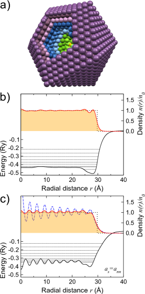
Figure 1: (Color online) a) Geometrical structure of 10-shell icosahedral Na${}_{2869}^{-}$ cluster. The next two panels show the electronic structure (only $\ell=0$ states are shown), the Kohn-Sham potential (black solid line), the electron density (red solid line) from the self-consistent local density approximation (LDA) calculations for the jellium model, the dotted line marks the ideal jellium background (b) and for the spherically averaged realistic ionic density (dashed blue line) (c). The intershell spacing is fixed at the bulk nearest neighbor distance.

In the present contribution we continue to study the optical properties of the magic Na${}_{2869}^{-}$ cluster (Fig. 1a). This system simultaneously possesses completely closed geometric and electronic shells. This makes it exceptionally stable and attractive for the numerical calculations: its electronic structure can be obtained easily by using the density functional approach. We do not pursue here a fully atomistic approach, but rather solve the radial Kohn-Sham equation (using the renormalized Numerov method) in the presence of the spherically symmetric ionic density. We either use the standard jellium model which starts from the homogeneous ionic density (Fig. 1b) or the density is obtained from the realistic geometric model by applying the gaussian broadening of $\sim 1$ Å width to ionic positions and performing a spherical averaging (Fig. 1c). In accordance with the proposed numerical scheme we present here a) the dipolar and the quadrupole linear optical absorption coefficients $\alpha_{\ell 0}(\omega)$ and the induced densities $\delta n^{(1)}_{\ell 0}(r;\omega)$ ($\ell=1,\,2$) (Fig. 2); b) results for the second-harmonic source $\xi^{(2)}(\mathbf{r})$; and c) the non-linear dipolar and quadrupole optical responses at $2\omega$ frequency (Fig. 3).

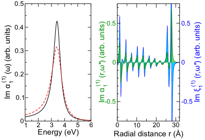
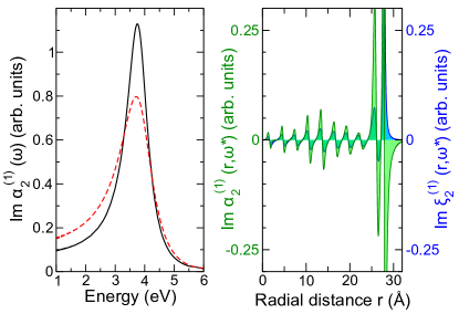
Figure 2: (Color online) The linear $\ell=1$ (top row) and $\ell=2$ (bottom row) optical response of the icosahedral Na${}_{2869}^{-}$ cluster based on the standard jellium model (black solid line) and on the model with the realistic ionic density (red dashed line). Right panels show the spatial dependence of the corresponding source terms $\xi^{(1)}_{\ell}(r,\omega^{*})$ and the resulting induced densities $\delta n^{(1)}_{\ell}(r,\omega^{*})$ for a particular frequency value $\omega^{*}=5.75$ eV.

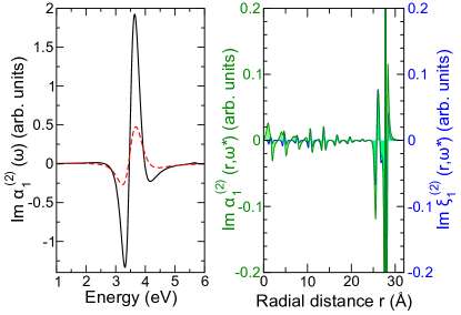
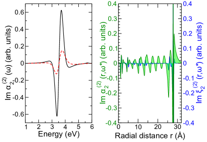
Figure 3: (Color online) The second-order non-linear $\ell=1$ (top row) and $\ell=2$ (bottom row) optical response of the icosahedral Na${}_{2869}^{-}$ cluster for the two models at Fig. 2. Right panels show the spatial dependence of the corresponding source terms $\xi^{(2)}_{\ell}(r,\omega^{*})$ and the resulting induced densities $\delta n^{(2)}_{\ell}(r,\omega^{*})$ for a particular frequency value $\omega^{*}=5.75$ eV.

While the linear optical response of metallic clusters is well understood: typically the optical absorption profile only slightly deviates from that of the idealistic system: a sphere filled with an electron gas of constant density. There, the optical absorption coefficient is peaked at the energies of the surface plasmon modes:

$$\omega_{\ell}=\sqrt{\frac{\ell}{2\ell+1}}\omega_{p}.$$

The position of the maxima is only weakly dependent on the details of the electronic structure: our calculations almost perfectly match corresponding idealistic values $\omega_{1}=3.45$ eV and $\omega_{2}=3.78$ eV for the bulk Na density ($r_{s}=3.96$). The spill-off of the electron density in realistic systems mostly leads to the broadening of the surface plasmon resonances. To illustrate this fact we choose the off-resonance value of the frequency ($\omega^{*}=5.75$ eV) and plot the source $\xi^{(2)}_{\ell}(r,\omega^{*})$ and the induced density $\delta n^{(2)}_{\ell}(r,\omega^{*})$ (Fig. 2). While in the idealistic situation the induced density is distributed over the surface of the sphere (where the electron density abruptly changes) in the realistic case we observe numerous features associated with slow electronic density variations within the cluster. They contribute to the optical absorption in the off-resonance regime. However, the relative weight of these oscillations decreases when the frequency approaches the resonance. There, the fast density variation at the surface dominates the spectrum.

The non-linear optical properties (Fig. 3) of even such simple systems are not fully understood. It is interesting to observe that two different excitation mechanisms (the quadrupole transition at $\omega$ or $2\omega$ frequency) lead to almost identical frequency dependence. Unlike in the linear case, the efficiency of the frequency conversion vanishes at the plasmon resonance and has two pronounced peaks at the energy slightly below and above. We also do not observe a strong correlation between the source and the induced density as in the off-resonant linear case (cf. blue and green curves). However, the spatial variation of these quantities is not erratic (as the plots might be suggesting). The complicated radial dependence is the result of the derivatives of the induced density and the potential in the non-linear source terms. Thanks to the linear-scaling algorithms we are using at each stage of the computation we are able to eliminate any spurious contributions from the numerical differentiation while ensuring the convergence of our results with respect to the number of discretization points and the value of the broadening parameter $\eta$.

V Conclusions

We developed a semi-classical theory of the second-harmonic generation in spherical particles. Although it originates from the exact quantum-mechanical sum-over-states expression and takes the local fields into account it is free from the small system size limitation. Because an efficient method for the solution of the corresponding integral equations exists the theory can be applied even to macroscopic systems provided the electronic density can be found. For this purpose the jellium approximation for the ionic density can be used as we illustrate by computing the SHG spectrum of the Na${}_{2869}^{-}$ cluster. The scattering cross-section and the angular distribution of the intensity are other important experimental observables. Calculation of these quantities will be presented elsewhere together with the inclusion of higher multipole moments allowing, thus, for the treatment of larger systems. The work along these lines is already in progress.

We believe that our method is sufficiently versatile as to allow for further extensions. In particular, it is straightforward to modify the method for systems with axial symmetry, or even to consider the symmetry-free case. To treat larger systems one must include higher multipole moments. This poses a question of how to find the second-order source term in this case. We believe that a direct manipulation with the maple computer algebra system rather than a formal solution in terms of $3j$ symbols is feasible.

Regarding the physical aspects of our approach: The fact that it is free of any adjustable parameters is not necessarily beneficial. In fact, for metallic systems with localized $d$-electrons peculiarities of the electronic structure might be reflected in the optical properties. In this case the classical electrodynamics approach with the experimentally measured dielectric function and susceptibility tensor might give more accurate results. On the other hand, for systems with simpler electronic structure our method is capable of taking into account quantum effects such as the spill-out of the electronic density.

Finally, our work establishes the equivalence between the semi-classical approximation and the hydrodynamic approach of Apell Apell (1983). The latter, however, is just a classical theory if not corrected for local field effects. We also touched upon the question of the representability of the response functions in terms of electronic densities and show that in general a more complicated quantity such as the one-particle density matrix must be introduced. However, for the second-harmonic generation these terms cancel in the final expression.

Appendix A Semi-classical expression for the first hyperpolarizability

We start with the expression for the second order non-linear response:

$$\chi_{2}^{(0)}(\mathbf{r};\mathbf{r}^{\prime},\mathbf{r}^{\prime\prime};\omega)=\sum_{i,j,k}\frac{\psi_{k}^{*}(\mathbf{r})\psi_{i}(\mathbf{r})\psi_{i}^{*}(\mathbf{r}^{\prime})\psi_{j}(\mathbf{r}^{\prime})\psi_{j}^{*}(\mathbf{r}^{\prime\prime})\psi_{k}(\mathbf{r}^{\prime\prime})}{2\omega+E_{i}-E_{k}+i\eta}\\ \times\left(\frac{f_{k}-f_{j}}{\omega+E_{j}-E_{k}+i\eta}-\frac{f_{j}-f_{i}}{\omega+E_{i}-E_{j}+i\eta}\right)$$ (30)

where $f$ is the Fermi function and $i$, $j$, $k$ refer to collections of quantum numbers that uniquely characterize electronic states of the system. In what follows we use the the following notations $E_{i}-E_{k}=E_{ik}$, $f_{i}-f_{k}=f_{ik}$, etc. The infinitesimally small positive number $\eta$ shifts the poles from the real axis and assures, thus, the causality of the response function. In what follows we will assume that it can be incorporated in the $\omega$ variable.

Let us consider a generic type of integrals:

$$\Phi(\mathbf{r})=\int\!d(\mathbf{r}^{\prime}\mathbf{r}^{\prime\prime})\chi_{2}^{(0)}(\mathbf{r};\mathbf{r}^{\prime},\mathbf{r}^{\prime\prime};\omega)\,\phi(\mathbf{r}^{\prime})\,\phi(\mathbf{r}^{\prime\prime})$$ (31)

and introduce our basic approximation. The semi-classical approximation (SCA) implies a high frequency condition $|E_{i}-E_{j}|\ll\omega$. Thus, the above expression can be expanded as a power series of $\omega$. The term proportional to $1/\omega^{2}$ in the expansion of $\Phi(\mathbf{r})$ vanishes in view of the completeness of the electron wave-functions:

$$\sum_{i}\psi^{*}_{i}(\mathbf{r}_{1})\psi_{i}(\mathbf{r}_{2})=\delta(\mathbf{r}_{1}-\mathbf{r}_{2}).$$ (32)

In what follows we will assume all wave-functions to be real. This can always be done without the loss of generality for time-invariant systems. Odd power terms vanish in view of the symmetry of the expression with respect to permutation $i\rightleftarrows k$ and $\mathbf{r}^{\prime}\rightleftarrows\mathbf{r}^{\prime\prime}$.

The $1/\omega^{4}$ term has the following form:

$$\Phi^{(4)}(\mathbf{r})=\int\!d(\mathbf{r}^{\prime}\mathbf{r}^{\prime\prime})\sum_{i,j,k}X_{i,j,k}(\mathbf{r},\mathbf{r}^{\prime},\mathbf{r}^{\prime\prime})\,\phi(\mathbf{r}^{\prime})\,\phi(\mathbf{r}^{\prime\prime})\\ \times\left[f_{kj}E_{kj}^{2}-\frac{1}{2}E_{ik}f_{kj}E_{kj}+\frac{1}{4}E_{ik}^{2}f_{kj}\right].$$ (33)

The first term vanishes after using the property (32), the integration over $\mathbf{r}^{\prime}$, and exploiting the permutation symmetry $j\rightleftarrows k$ and $\mathbf{r}\rightleftarrows\mathbf{r}^{\prime\prime}$ of the expression under the integral. The term proportional to $E^{2}_{ik}f_{j}$ can be re-written as $2E_{ik}E_{jk}f_{j}$ and combined with the second terms. Finally our expression can be written as:

$$\Phi^{(4)}(\mathbf{r})=\frac{1}{4}\Phi^{(4a)}(\mathbf{r})-\Phi^{(4b)}(\mathbf{r})+\frac{1}{2}\Phi^{(4c)}(\mathbf{r})$$ (34)

with following notations:

$$\Phi^{(4a)}(\mathbf{r}) = \int\!d(\mathbf{r}^{\prime}\mathbf{r}^{\prime\prime})\sum_{i,j,k}X_{i,j,k}(\mathbf{r},\mathbf{r}^{\prime},\mathbf{r}^{\prime\prime})\Big{[}E_{ik}^{2}f_{k}\Big{]}\phi(\mathbf{r}^{\prime})\,\phi(\mathbf{r}^{\prime\prime}),$$

$$\Phi^{(4b)}(\mathbf{r}) = \int\!d(\mathbf{r}^{\prime}\mathbf{r}^{\prime\prime})\sum_{i,j,k}X_{i,j,k}(\mathbf{r},\mathbf{r}^{\prime},\mathbf{r}^{\prime\prime})\Big{[}E_{ik}E_{jk}f_{j}\Big{]}\phi(\mathbf{r}^{\prime})\,\phi(\mathbf{r}^{\prime\prime}),$$

$$\Phi^{(4c)}(\mathbf{r}) = \int\!d(\mathbf{r}^{\prime}\mathbf{r}^{\prime\prime})\sum_{i,j,k}X_{i,j,k}(\mathbf{r},\mathbf{r}^{\prime},\mathbf{r}^{\prime\prime})\Big{[}E_{ik}E_{jk}f_{k}\Big{]}\phi(\mathbf{r}^{\prime})\,\phi(\mathbf{r}^{\prime\prime}).$$

In what follows we will make use of

$$E_{ij}\psi_{i}(\mathbf{r})\psi_{j}(\mathbf{r})=-\frac{1}{2}\mathbf{\nabla}\cdot\boldsymbol{\xi}_{ij}(\mathbf{r}),$$ (35)

where $\boldsymbol{\xi}_{ij}(\mathbf{r})=\psi_{j}(\mathbf{r})\mathbf{\nabla}\psi_{i}(\mathbf{r})-\psi_{i}(\mathbf{r})\mathbf{\nabla}\psi_{j}(\mathbf{r})$. This follows from the Schrödinger equation.

Let us consider first the $\Phi^{(4a)}(\mathbf{r})$ term. After the summation over $j$ and integration over $\mathbf{r}^{\prime\prime}$ we arrive at:

$$\Phi^{(4a)}(\mathbf{r})=\frac{1}{4}\int\!d\mathbf{r}^{\prime}\phi^{2}(\mathbf{r}^{\prime})\sum_{i,k}f_{k}[\mathbf{\nabla}_{r}\cdot\boldsymbol{\xi}_{ik}(\mathbf{r})][\mathbf{\nabla}_{r^{\prime}}\cdot\boldsymbol{\xi}_{ik}(\mathbf{r}^{\prime})].$$

We further pull $\mathbf{\nabla}_{r}$ out of the integration and use the Gauss theorem to apply $\mathbf{\nabla}_{r^{\prime}}$ to the $\phi^{2}(\mathbf{r}^{\prime})$:

$$\Phi^{(4a)}=-\frac{\mathbf{\nabla}_{r}}{4}\cdot\int\!d\mathbf{r}^{\prime}\sum_{i,k}f_{k}\,\boldsymbol{\xi}_{ik}(\mathbf{r})\,[\boldsymbol{\xi}_{ik}(\mathbf{r}^{\prime})\cdot\mathbf{\nabla}_{r^{\prime}}\phi^{2}(\mathbf{r}^{\prime})].$$ (36)

Now the summation over $i$ and $k$ can be performed by introducing the one-particle density matrix:

$$\sum_{i}f_{i}\psi_{i}(\mathbf{r}_{1})\psi_{i}(\mathbf{r}_{2})=\gamma(\mathbf{r}_{1},\mathbf{r}_{2}),$$ (37)

with the diagonal elements given by the density:

$$\sum_{i}f_{i}\psi_{i}(\mathbf{r})\psi_{i}(\mathbf{r})=n(\mathbf{r}),$$ (38)

Quite general we can represent the density matrix in the form:

$$\gamma(\mathbf{r}_{1},\mathbf{r}_{2})=f(\mathbf{r}_{1})\,f(\mathbf{r}_{2})g(|\mathbf{r}_{1}-\mathbf{r}_{2}|).$$

From the definition (37) a useful integration formula can be derived:

$$\int\!d\mathbf{r}^{\prime}\delta(\mathbf{r}-\mathbf{r}^{\prime})F(\mathbf{r}^{\prime})\mathbf{\nabla}_{r}\gamma(\mathbf{r},\mathbf{r}^{\prime})\\ =\int\!d\mathbf{r}^{\prime}\delta(\mathbf{r}-\mathbf{r}^{\prime})F(\mathbf{r}^{\prime})\mathbf{\nabla}_{r^{\prime}}\gamma(\mathbf{r},\mathbf{r}^{\prime})=\frac{1}{2}F(\mathbf{r})\mathbf{\nabla}_{r}n(\mathbf{r}).$$ (39)

Let us now return to (36) and perform the sum over the states using eqs. 37 and 38.

$$\Phi^{(4a)}=-\frac{1}{4}\sum_{ab}\nabla_{r}^{a}\int\!d\mathbf{r}^{\prime}\nabla_{r^{\prime}}\phi^{2}(\mathbf{r}^{\prime})\\ \times\Big{[}\gamma(\mathbf{r},\mathbf{r}^{\prime})\nabla_{r}^{a}\nabla_{r^{\prime}}^{b}\delta(\mathbf{r},\mathbf{r}^{\prime})-\nabla_{r}^{a}\gamma(\mathbf{r},\mathbf{r}^{\prime})\nabla_{r^{\prime}}^{b}\delta(\mathbf{r},\mathbf{r}^{\prime})\\ -\nabla_{r}^{a}\delta(\mathbf{r},\mathbf{r}^{\prime})\nabla_{r^{\prime}}^{b}\gamma(\mathbf{r},\mathbf{r}^{\prime})+\delta(\mathbf{r},\mathbf{r}^{\prime})\nabla_{r}^{a}\nabla_{r^{\prime}}^{b}\gamma(\mathbf{r},\mathbf{r}^{\prime})\Big{]}.$$ (40)

In order to evaluate the integral we must remove all differential operators from the $\delta$-function.

$$\Phi^{(4a)}=-\frac{1}{4}\sum_{ab}\nabla_{r}^{a}\int\!d\mathbf{r}^{\prime}\nabla_{r^{\prime}}^{b}\phi^{2}(\mathbf{r}^{\prime})\\ \times\Big{[}\nabla_{r^{\prime}}^{b}\nabla_{r}^{a}[\delta(\mathbf{r},\mathbf{r}^{\prime})\gamma(\mathbf{r},\mathbf{r}^{\prime})]-2\nabla_{r}^{a}[\delta(\mathbf{r},\mathbf{r}^{\prime})\nabla_{r^{\prime}}^{b}\gamma(\mathbf{r},\mathbf{r}^{\prime})]\\ -2\nabla_{r^{\prime}}^{b}[\delta(\mathbf{r},\mathbf{r}^{\prime})\nabla_{r}^{a}\gamma(\mathbf{r},\mathbf{r}^{\prime})]+4\delta(\mathbf{r},\mathbf{r}^{\prime})\nabla_{r}^{a}\nabla_{r^{\prime}}^{b}\gamma(\mathbf{r},\mathbf{r}^{\prime})\Big{]}.$$ (41)

It can be further simplified by using Green’s first identity for the first and third terms:

$$\Phi^{(4a)}=\frac{\Delta}{4}\int\!d\mathbf{r}^{\prime}\delta(\mathbf{r},\mathbf{r}^{\prime})\Big{[}\Delta\phi^{2}(\mathbf{r}^{\prime})\gamma(\mathbf{r},\mathbf{r}^{\prime})\\ +2\nabla_{r^{\prime}}^{b}\phi^{2}(\mathbf{r}^{\prime})\nabla_{r^{\prime}}^{b}\gamma(\mathbf{r},\mathbf{r}^{\prime})\Big{]}\\ -\frac{1}{2}\sum_{a}\nabla_{r}^{a}\int\!d\mathbf{r}^{\prime}\delta(\mathbf{r},\mathbf{r}^{\prime})\Big{[}\Delta[\phi^{2}(\mathbf{r}^{\prime})]\nabla_{r}^{a}\gamma(\mathbf{r},\mathbf{r}^{\prime})\\ +2\sum_{b}\nabla_{r}^{a}\nabla_{r^{\prime}}^{b}\gamma(\mathbf{r},\mathbf{r}^{\prime})\nabla_{r^{\prime}}^{b}\phi^{2}(\mathbf{r}^{\prime})\Big{]}.$$ (42)

Let us introduce the tensor $\mathbb{T}^{ab}(\mathbf{r})=\lim_{\mathbf{r}^{\prime}\rightarrow\mathbf{r}}\nabla_{r}^{a}\nabla_{r^{\prime}}^{b}\gamma(\mathbf{r},\mathbf{r}^{\prime})$ and integrate:

$$\Phi^{(4a)}=\frac{1}{4}\Delta\Big{[}n\,\Delta\phi^{2}+(\mathbf{\nabla}\phi^{2}\cdot\mathbf{\nabla}n)\Big{]}\\ -\frac{1}{4}\mathbf{\nabla}\cdot\Big{[}\mathbf{\nabla}n\,\Delta\phi^{2}\Big{]}-\sum_{ab}\nabla^{a}\Big{[}\mathbb{T}^{ab}\nabla^{b}\phi^{2}\Big{]}.$$ (43)

Using (35) we re-write $\Phi^{(4b)}$ in the form without explicit energies:

$$\Phi^{(4b)}(\mathbf{r})=\frac{\mathbf{\nabla}_{r}}{4}\cdot\int\!d(\mathbf{r}^{\prime}\mathbf{r}^{\prime\prime})\,\phi(\mathbf{r}^{\prime})\phi(\mathbf{r}^{\prime\prime})\sum_{i,j,k}f_{j}\boldsymbol{\xi}_{ik}(r)\big{[}\mathbf{\nabla}_{r^{\prime\prime}}\cdot\boldsymbol{\xi}_{jk}\big{]}\\ \times\psi_{i}(\mathbf{r}^{\prime})\psi_{j}(\mathbf{r}^{\prime}).$$ (44)

We perform the summations over the states and use the Gauss theorem to transfer $\mathbf{\nabla}_{r^{\prime\prime}}$ on $\phi(\mathbf{r}^{\prime\prime})$ to obtain

$$\Phi^{(4b)}(\mathbf{r})=-\frac{1}{4}\sum_{ab}\nabla_{r}^{a}\int\!d(\mathbf{r}^{\prime}\mathbf{r}^{\prime\prime})\phi(\mathbf{r}^{\prime})\,\nabla_{r^{\prime\prime}}^{b}\phi(\mathbf{r}^{\prime\prime})\\ \times\Big{[}\delta(\mathbf{r},\mathbf{r}^{\prime\prime})\nabla_{r}^{a}\delta(\mathbf{r},\mathbf{r}^{\prime})\,\nabla_{r^{\prime\prime}}^{b}\gamma(\mathbf{r}^{\prime\prime},\mathbf{r}^{\prime})\\ -\nabla_{r^{\prime\prime}}^{b}\delta(\mathbf{r},\mathbf{r}^{\prime\prime})\,\nabla_{r}^{a}\delta(\mathbf{r},\mathbf{r}^{\prime})\,\gamma(\mathbf{r}^{\prime\prime},\mathbf{r}^{\prime})\\ -\nabla_{r}^{a}\delta(\mathbf{r},\mathbf{r}^{\prime\prime})\,\delta(\mathbf{r},\mathbf{r}^{\prime})\,\nabla_{r^{\prime\prime}}^{b}\gamma(\mathbf{r}^{\prime\prime},\mathbf{r}^{\prime})\\ +\nabla_{r^{\prime\prime}}^{b}\nabla_{r}^{a}\Big{(}\delta(\mathbf{r},\mathbf{r}^{\prime\prime})\Big{)}\,\delta(\mathbf{r},\mathbf{r}^{\prime})\,\gamma(\mathbf{r}^{\prime\prime},\mathbf{r}^{\prime})\Big{]}$$ (45)

The integration yields:

$$\Phi^{(4b_{1})}(\mathbf{r}) = -\frac{1}{4}\sum_{ab}\nabla_{r}^{a}\Big{[}\nabla_{r}^{b}\phi(\mathbf{r})\nabla_{r}^{a}\int\!d\mathbf{r}^{\prime}\phi(\mathbf{r}^{\prime})\delta(\mathbf{r},\mathbf{r}^{\prime})\,\nabla_{r}^{b}\gamma(\mathbf{r},\mathbf{r}^{\prime})$$

$$+\frac{1}{4}\sum_{ab}\nabla_{r}^{a}\Big{[}\nabla_{r}^{b}\phi(\mathbf{r})\!\int\!d\mathbf{r}^{\prime}\phi(\mathbf{r}^{\prime})\,\delta(\mathbf{r},\mathbf{r}^{\prime})\,\nabla_{r}^{a}\nabla_{r}^{b}\gamma(\mathbf{r},\mathbf{r}^{\prime})\Big{]}$$

$$= -\frac{1}{4}\sum_{a}\nabla^{a}\Big{[}\frac{1}{2}(\nabla n\cdot\nabla\phi)\nabla^{a}\phi+\phi\sum_{b}\mathbb{T}^{ab}\nabla^{b}\phi\Big{]},$$

$$\Phi^{(4b_{3})}(\mathbf{r}) = \frac{1}{8}\sum_{a}\nabla^{a}\Big{[}\phi\nabla^{a}(\nabla\phi\cdot\nabla n)-2\phi\sum_{b}\mathbb{T}^{ab}\nabla^{b}\phi\Big{]},$$

$$\Phi^{(4b_{4})}(\mathbf{r}) = -\frac{1}{4}\sum_{ab}\nabla_{r}^{a}\Big{[}\phi(\mathbf{r})\!\!\int\!d\mathbf{r}^{\prime\prime}\nabla_{r^{\prime\prime}}^{b}\phi(\mathbf{r}^{\prime\prime})\,\gamma(\mathbf{r}^{\prime\prime},\mathbf{r})\,\nabla_{r^{\prime\prime}}^{b}\nabla_{r}^{a}\delta(\mathbf{r},\mathbf{r}^{\prime\prime})\Big{]}$$

$$= -\frac{1}{4}\sum_{ab}\nabla_{r}^{a}\Big{[}\phi(\mathbf{r})\nabla_{r}^{a}\!\!\int\!d\mathbf{r}^{\prime\prime}\nabla_{r^{\prime\prime}}^{b}\phi(\mathbf{r}^{\prime\prime})\,\gamma(\mathbf{r}^{\prime\prime},\mathbf{r})\,\nabla_{r^{\prime\prime}}^{b}\delta(\mathbf{r},\mathbf{r}^{\prime\prime})\Big{]}$$

$$+ \frac{1}{4}\sum_{ab}\nabla_{r}^{a}\Big{[}\phi(\mathbf{r})\!\int\!d\mathbf{r}^{\prime\prime}\nabla_{r^{\prime\prime}}^{b}\phi(\mathbf{r}^{\prime\prime})\,\nabla_{r}^{a}\gamma(\mathbf{r}^{\prime\prime},\mathbf{r})\,\nabla_{r^{\prime\prime}}^{b}\delta(\mathbf{r},\mathbf{r}^{\prime\prime})\Big{]}.$$

The $\Phi^{(4b_{4})}(\mathbf{r})$ term requires special attention:

$$\Phi^{(4b_{4})}(\mathbf{r})$$

$$= -\frac{1}{4}\sum_{ab}\nabla_{r}^{a}\Big{[}\phi(\mathbf{r})\nabla_{r}^{a}\!\int\!d\mathbf{r}^{\prime\prime}\nabla_{r^{\prime\prime}}^{b}\phi(\mathbf{r}^{\prime\prime})\,\nabla_{r^{\prime\prime}}^{b}\big{[}\delta(\mathbf{r},\mathbf{r}^{\prime\prime})\gamma(\mathbf{r}^{\prime\prime},\mathbf{r})\big{]}\Big{]}$$

$$+ \frac{1}{4}\sum_{ab}\nabla_{r}^{a}\Big{[}\phi(\mathbf{r})\nabla_{r}^{a}\!\int\!d\mathbf{r}^{\prime\prime}\delta(\mathbf{r},\mathbf{r}^{\prime\prime})\,\nabla_{r^{\prime\prime}}^{b}\phi(\mathbf{r}^{\prime\prime})\,\nabla_{r^{\prime\prime}}^{b}\gamma(\mathbf{r}^{\prime\prime},\mathbf{r})\Big{]}$$

$$+ \frac{1}{4}\sum_{ab}\nabla_{r}^{a}\Big{[}\phi(\mathbf{r})\!\int\!d\mathbf{r}^{\prime\prime}\nabla_{r^{\prime\prime}}^{b}\phi(\mathbf{r}^{\prime\prime})\,\nabla_{r^{\prime\prime}}^{b}\big{[}\delta(\mathbf{r},\mathbf{r}^{\prime\prime})\nabla_{r}^{a}\gamma(\mathbf{r}^{\prime\prime},\mathbf{r})\big{]}\Big{]}$$

$$- \frac{1}{4}\sum_{ab}\nabla_{r}^{a}\Big{[}\phi(\mathbf{r})\!\int\!d\mathbf{r}^{\prime\prime}\delta(\mathbf{r},\mathbf{r}^{\prime\prime})\,\nabla_{r^{\prime\prime}}^{b}\phi(\mathbf{r}^{\prime\prime})\,\nabla_{r^{\prime\prime}}^{b}\nabla_{r}^{a}\gamma(\mathbf{r}^{\prime\prime},\mathbf{r})\Big{]}$$

$$= \frac{1}{8}\sum_{a}\nabla^{a}\Big{[}\phi\nabla^{a}(\nabla\phi\cdot\nabla n)-2\sum_{b}\phi\mathbb{T}^{ab}\nabla^{b}\phi\Big{]}$$

$$+ \frac{1}{8}\sum_{a}\nabla^{a}\Big{[}2\phi\nabla^{a}\big{(}n\Delta\phi\big{)}-\phi\Delta\phi\nabla^{a}n\Big{]}.$$

$$\Phi^{(4b_{2})}(\mathbf{r})$$

$$= \frac{1}{4}\Delta\sum_{b}\int\!d(\mathbf{r}^{\prime}\mathbf{r}^{\prime\prime})\,\phi(\mathbf{r}^{\prime})\,\nabla_{r^{\prime\prime}}^{b}\phi(\mathbf{r}^{\prime\prime})\,\nabla_{r^{\prime\prime}}^{b}\delta(\mathbf{r},\mathbf{r}^{\prime\prime})$$

$$\times \delta(\mathbf{r},\mathbf{r}^{\prime})\,\gamma(\mathbf{r}^{\prime\prime},\mathbf{r}^{\prime})+\Phi^{(4b_{4})}(\mathbf{r})$$

$$= \frac{1}{4}\Delta\left[\phi\!\!\int\!d\mathbf{r}^{\prime\prime}\sum_{b}\nabla_{r^{\prime\prime}}^{b}\phi(\mathbf{r}^{\prime\prime})\,\nabla_{r^{\prime\prime}}^{b}\Big{[}\delta(\mathbf{r},\mathbf{r}^{\prime\prime})\gamma(\mathbf{r}^{\prime\prime},\mathbf{r})\Big{]}\right]$$

$$- \frac{1}{4}\Delta\left[\phi\!\!\int\!d\mathbf{r}^{\prime\prime}\sum_{b}\nabla_{r^{\prime\prime}}^{b}\phi(\mathbf{r}^{\prime\prime})\,\nabla_{r^{\prime\prime}}^{b}\gamma(\mathbf{r}^{\prime\prime},\mathbf{r})\,\delta(\mathbf{r},\mathbf{r}^{\prime\prime})\right]+\Phi^{(4b_{4})}(\mathbf{r})$$

$$= -\frac{1}{4}\Delta\Big{[}\phi n\Delta\phi+\frac{1}{2}\phi(\nabla n\cdot\nabla\phi)\Big{]}+\Phi^{(4b_{4})}(\mathbf{r}).$$

Combining together we obtain:

$$\Phi^{(4b)}(\mathbf{r})=-\frac{1}{4}\Delta\Big{[}\phi\,(\nabla\phi\cdot\nabla n)\Big{]}+\frac{1}{2}\mathbf{\nabla}\cdot\Big{[}\phi\mathbf{\nabla}\big{(}\mathbf{\nabla}n\cdot\mathbf{\nabla}\phi\big{)}\Big{]}\\ -\frac{1}{4}\Delta\Big{[}\phi n\Delta\phi\Big{]}+\frac{1}{2}\mathbf{\nabla}\cdot\Big{[}\phi\mathbf{\nabla}(n\Delta\phi)\Big{]}\\ -\sum_{a}\nabla^{a}\Big{[}\phi\mathbb{T}^{ab}\nabla^{b}\phi\Big{]}-\frac{1}{4}\mathbf{\nabla}\cdot\Big{[}\phi\Delta\phi\mathbf{\nabla}n\Big{]}.$$ (46)

Equation for $\Phi^{(4c)}$ is obtained from (45) with replacement $\delta(\mathbf{r},\mathbf{r}^{\prime\prime})\rightarrow\gamma(\mathbf{r},\mathbf{r}^{\prime\prime})$ and $\gamma(\mathbf{r}^{\prime\prime},\mathbf{r}^{\prime})\rightarrow\delta(\mathbf{r}^{\prime\prime},\mathbf{r}^{\prime})$:

$$\Phi^{(4c)}(\mathbf{r})=-\frac{1}{4}\sum_{ab}\nabla_{r}^{a}\int\!d(\mathbf{r}^{\prime}\mathbf{r}^{\prime\prime})\phi(\mathbf{r}^{\prime})\,\nabla_{r^{\prime\prime}}^{b}\phi(\mathbf{r}^{\prime\prime})\\ \times\Big{[}\gamma(\mathbf{r},\mathbf{r}^{\prime\prime})\,\nabla_{r}^{a}\delta(\mathbf{r},\mathbf{r}^{\prime})\,\nabla_{r^{\prime\prime}}^{b}\delta(\mathbf{r}^{\prime\prime},\mathbf{r}^{\prime})\\ -\nabla_{r^{\prime\prime}}^{b}\gamma(\mathbf{r},\mathbf{r}^{\prime\prime})\,\nabla_{r}^{a}\delta(\mathbf{r},\mathbf{r}^{\prime})\,\delta(\mathbf{r}^{\prime\prime},\mathbf{r}^{\prime})\\ -\nabla_{r}^{a}\gamma(\mathbf{r},\mathbf{r}^{\prime\prime})\,\delta(\mathbf{r},\mathbf{r}^{\prime})\,\nabla_{r^{\prime\prime}}^{b}\delta(\mathbf{r}^{\prime\prime},\mathbf{r}^{\prime})\\ +\nabla_{r^{\prime\prime}}^{b}\nabla_{r}^{a}\Big{(}\gamma(\mathbf{r},\mathbf{r}^{\prime\prime})\Big{)}\,\delta(\mathbf{r},\mathbf{r}^{\prime})\,\delta(\mathbf{r}^{\prime\prime},\mathbf{r}^{\prime})\Big{]}.$$ (47)

Integrations yield:

$$\Phi^{(4c_{4})}(\mathbf{r}) = -\frac{1}{4}\sum_{ab}\nabla^{a}\Big{[}\phi\mathbb{T}^{ab}\nabla^{b}\phi\Big{]},$$

$$\Phi^{(4c_{3})}(\mathbf{r}) = -\frac{1}{4}\sum_{ab}\nabla_{r}^{a}\phi\int\!d\mathbf{r}^{\prime\prime}\nabla_{r^{\prime\prime}}^{b}\phi(\mathbf{r}^{\prime\prime})\,\nabla_{r}^{a}\gamma(\mathbf{r},\mathbf{r}^{\prime\prime})\,\nabla_{r^{\prime\prime}}^{b}\delta(\mathbf{r}^{\prime\prime},\mathbf{r})$$

$$= +\frac{1}{8}\sum_{a}\nabla^{a}\Big{[}\phi\Delta\phi\nabla^{a}n+2\phi\sum_{b}\mathbb{T}^{ab}\nabla^{b}\phi\Big{]},$$

$$\Phi^{(4c_{2})}(\mathbf{r}) = \frac{1}{4}\sum_{ab}\nabla_{r}^{a}\int\!d\mathbf{r}^{\prime}\,\phi(\mathbf{r}^{\prime})\,\nabla_{r^{\prime}}^{b}\phi(\mathbf{r}^{\prime})\,\nabla_{r^{\prime}}^{b}\gamma(\mathbf{r},\mathbf{r}^{\prime})\,\nabla_{r}^{a}\delta(\mathbf{r},\mathbf{r}^{\prime})$$

$$= \frac{1}{8}\Delta\Big{[}\phi(\nabla\phi\cdot\nabla n)\Big{]}-\frac{1}{4}\sum_{ab}\nabla^{a}\Big{[}\phi\mathbb{T}^{ab}\nabla^{b}\phi\Big{]}.$$

It is little bit more difficult to get the first term:

$$\Phi^{(4c_{1})}(\mathbf{r}) = -\frac{1}{4}\Delta\Big{[}\phi\int\!d\mathbf{r}^{\prime\prime}\,\gamma(\mathbf{r},\mathbf{r}^{\prime\prime})\sum_{b}\nabla_{r^{\prime\prime}}^{b}\phi(\mathbf{r}^{\prime\prime})\,\nabla_{r^{\prime\prime}}^{b}\delta(\mathbf{r}^{\prime\prime},\mathbf{r})\Big{]}$$

$$+ \frac{1}{4}\sum_{ab}\nabla_{r}^{a}\phi\int\!d\mathbf{r}^{\prime\prime}\,\nabla_{r^{\prime\prime}}^{b}\phi(\mathbf{r}^{\prime\prime})\,\nabla_{r}^{a}\gamma(\mathbf{r},\mathbf{r}^{\prime\prime})\,\nabla_{r^{\prime\prime}}^{b}\delta(\mathbf{r}^{\prime\prime},\mathbf{r})$$

$$= \frac{1}{4}\Delta\Big{[}\phi n\Delta\phi\Big{]}+\frac{1}{8}\Delta\Big{[}\phi(\nabla\phi\cdot\nabla n)\Big{]}$$

$$- \frac{1}{8}\sum_{a}\nabla^{a}\Big{[}\phi\Delta\phi\nabla^{a}n\Big{]}-\frac{1}{4}\sum_{ab}\nabla^{a}\Big{[}\phi\mathbb{T}^{ab}\nabla^{b}\phi\Big{]}.$$

Combining together we obtain:

$$\Phi^{(4c)}(\mathbf{r})=\frac{1}{4}\Delta\Big{[}\phi\,(\nabla\phi\cdot\nabla n)\Big{]}+\frac{1}{4}\Delta\Big{[}\phi n\Delta\phi\Big{]}\\ -\sum_{a}\nabla^{a}\Big{[}\phi\mathbb{T}^{ab}\nabla^{b}\phi\Big{]}-\frac{1}{4}\mathbf{\nabla}\cdot\Big{[}\phi\Delta\phi\mathbf{\nabla}n\Big{]}.$$ (48)

Finally substituting eqs. 43, 46 and 48 in (34) we obtain for the forth order term:

$$\Phi^{(4)}(\mathbf{r})=\frac{1}{2}\mathbf{\nabla}\cdot\Big{[}\mathbf{\nabla}\phi\,\Big{(}n\Delta\phi+(\nabla\phi\cdot\nabla n)\Big{)}+\frac{1}{4}n\mathbf{\nabla}\big{(}\mathbf{\nabla}\phi\big{)}^{2}\Big{]}.$$ (49)

$\Phi(\mathbf{r})$ has the meaning of an induced density, i.e. it is a gradient of the non-linear polarization. Expression for this quantity was derived by Wang, Cheng and Bower Wang et al. (1973) and Apell Apell (1983) from the classical equation of motion for the electron in electromagnetic fields. Our expression is identical to their result (cf. Eq. (11) in Wang et al. (1973); Apell (1983)) if we write the external field in the form $\mathbf{E}=-\mathbf{\nabla}\phi$. Our expression is more general in a sense that $\mathbf{E}$ also contains the induced fields. Note there are no more terms containing $\gamma(\mathbf{r},\mathbf{r}^{\prime\prime})$ in the expression (49). The high-frequency condition is not the only way to simplify Eq. (30). In particular, Rudnick and Stern Rudnick and Stern (1971) demonstrated another possibility to arrive at the classical expression (Eq. (1)) starting from the quantum mechanical response function for the homogeneous electron gas and applying the local approximation $qv_{F}\ll\omega$, where $v_{F}$ is the Fermi velocity and $q$ is the inverse of the characteristic length of variation of the field.

Appendix B Non-linear source term $\xi^{(2b)}_{\ell 0}(r)$

Here we present expressions for the second part of the second-harmonic source term. Calculations are facilitated by the use of maple computer algebra package.

$$\xi^{(2b)}_{1}=-\frac{1}{4\omega^{4}\sqrt{5\pi}}\Bigg{[}\frac{6f_{1}f_{2}}{r^{4}}\Big{(}rn^{\prime}-8n\Big{)}+\frac{24n}{r^{3}}\Big{(}f_{1}f_{2}^{\prime}+2f_{2}f_{1}^{\prime}\Big{)}\\ +\frac{4\pi n}{r^{2}}\Big{(}7f_{1}n_{2}+15n_{1}f_{2}\Big{)}-\frac{n^{\prime}}{r^{2}}\Big{(}5f_{1}f_{2}^{\prime}+9f_{2}f_{1}^{\prime}\Big{)}\\ +\frac{4\pi}{r}\Big{(}rn^{\prime}-4n\Big{)}\Big{(}n_{1}f_{2}^{\prime}+n_{2}f_{1}^{\prime}+\frac{f_{1}^{\prime}f_{2}^{\prime}}{\pi r}\Big{)}\\ +4\pi n\Big{(}f_{1}^{\prime}n_{2}^{\prime}+f_{2}^{\prime}n_{1}^{\prime}-8\pi n_{1}n_{2}\Big{)}\Bigg{]},$$ (50)

$$\xi^{(2b)}_{2}=-\frac{1}{4\omega^{4}\sqrt{5\pi}}\Bigg{[}4\pi n\Big{(}f_{1}^{\prime}n_{1}^{\prime}-4\pi n_{1}^{2}\Big{)}+\frac{4\pi n}{r^{3}}\Big{(}3rf_{1}n_{1}-4f_{1}^{\prime}n_{1}\Big{)}\\ +\frac{8nf_{1}^{\prime}f_{1}}{r^{3}}-\frac{4n}{r^{4}}\Big{(}f_{1}^{2}+r^{2}(f_{1}^{\prime})^{2}\Big{)}\\ +n^{\prime}\Big{(}4\pi n_{1}f_{1}^{\prime}+\frac{2(f_{1}^{\prime})^{2}}{r}-\frac{f_{1}f_{1}^{\prime}}{r^{2}}-\frac{f_{1}^{2}}{r^{3}}\Big{)}\Bigg{]}.$$ (51)

We use the same abbreviated notations as in Sec. III and additionally introduce $\xi^{(2b)}_{\ell}\equiv\xi^{(2b)}_{\ell 0}$, $n\equiv n(r)$.

Appendix C Fast numerical solution of the integral equation

It is convenient to recast eqs. 24 and 25 in the following form:

$$\alpha_{\ell}(r;\omega)=\xi_{\ell}(r;\omega)-\alpha^{(0)}_{\ell}(r;\omega)\\ \times\int_{0}^{\infty}dr^{\prime}\left(\frac{1}{r^{\prime}}\right)^{\ell-1}\!G^{\text{sph}}_{\ell}(r,r^{\prime})\,\alpha_{\ell}(r^{\prime};\omega),$$ (52)

where for the linear response we have $\xi_{\ell}(r;\omega)=\ell\alpha^{(0)}_{\ell}(r;\omega)$. Let us now omit the $\omega$ argument for simpification and use the definition (23):

$$\alpha_{\ell}(r)=\xi_{\ell}(r)+\alpha^{(0)}_{\ell}(r)\Big{[}\ell\,a-\frac{\ell+1}{r^{2\ell+1}}w_{1}(r)-\ell w_{2}(r)\Big{]},$$

with

$$w_{1}(r) = \int_{0}^{r}\Big{(}r^{\prime}\Big{)}^{\ell+2}\alpha_{\ell}(r^{\prime})\,dr^{\prime},$$

$$w_{2}(r) = \int_{0}^{r}\left(\frac{1}{r^{\prime}}\right)^{\ell-1}\!\!\!\alpha_{\ell}(r^{\prime})\,dr^{\prime},\quad\text{and}\quad a=w_{2}(\infty).$$

Functions $w_{1,2}(r)$ satisfy following differential equations:

$$w^{\prime}_{1}(r) = r^{\ell+2}\Bigg{\{}\xi_{\ell}(r)+\alpha^{(0)}_{\ell}(r)\,\Big{[}\ell\,a-\frac{\ell+1}{r^{2\ell+1}}w_{1}(r)-\ell w_{2}(r)\Big{]}\Bigg{\}},$$

$$w^{\prime}_{2}(r) = \frac{1}{r^{\ell-1}}\Bigg{\{}\xi_{\ell}(r)+\alpha^{(0)}_{\ell}(r)\,\Big{[}\ell\,a-\frac{\ell+1}{r^{2\ell+1}}w_{1}(r)-\ell w_{2}(r)\Big{]}\Bigg{\}}.$$

They can be solved at the $\mathcal{O}(N)$ cost where $N$ is the number of mesh points to represent the density.

References

Mahan (2000)G. Mahan, Many-particle
physics, 3rd ed. (Kluwer
Academic/Plenum Publishers, New York, 2000).
Halas et al. (2011)N. J. Halas, S. Lal, W. Chang, S. Link, and P. Nordlander, Chem. Rev., 111, 3913 (2011).
Ward (1965)J. F. Ward, Rev.
Mod. Phys., 37, 1
(1965).
Wang and Carter (2002)Y. Wang and E. Carter, in Theoretical Methods in
Condensed Phase Chemistry, Progress in
Theoretical Chemistry and Physics (Kluwer Academic
Publishers, Dordrecht, 2002) pp. 117–184.
Liebsch and Schaich (1989)A. Liebsch and W. L. Schaich, Phys.
Rev. B, 40, 5401
(1989).
Zangwill and Soven (1980)A. Zangwill and P. Soven, Phys.
Rev. A, 21, 1561
(1980).
Jackson (1999)J. Jackson, Classical
electrodynamics, 3rd ed. (Wiley, New York, 1999).
Rudnick and Stern (1971)J. Rudnick and E. A. Stern, Phys.