EFFECTS OF CLASSICAL ENVIRONMENTAL NOISE
ON ENTANGLEMENT AND QUANTUM DISCORD DYNAMICS

Abstract

We address the effect of classical noise on the dynamics of quantum correlations, entanglement and quantum discord, of two non-interacting qubits initially prepared in a Bell state. The effect of noise is modeled by randomizing the single-qubit transition amplitudes. We address both static and dynamic environmental noise corresponding to interaction with separate common baths in either Markovian and non-Markovian regimes. In the Markov regime, a monotone decay of the quantum correlations is found, whereas for non-Markovian noise sudden death and revival phenomena may occur, depending on the characteristics of the noise. Entanglement and quantum discord show the same qualitative behavior for all kind of noises considered. On the other hand, we find that separate and common environments may play opposite roles in preserving quantum correlations, depending on the noise regime considered.

1 Introduction

Quantum entanglement is a fundamental resource for quantum information processing, communication and exponential speed-up of some computational tasks [1, 2]. As a consequence, in the last years, there has been an increasing interest in quantum correlations in various physical fields, ranging from quantum optics [3, 4, 5, 6] to nanophysics [7, 8]. Furthemore, recently, it was pointed out that nonclassical correlations exist which are more general, and possibly more fundamental then entanglement [9, 10, 11], the so-called quantum discord (QD), which is defined as the difference between total and classical correlations in a system. Under suitable conditions QD has been proved to be more robust than entanglement with respect to decoherence [12, 13]. Decoherence is indeed the main threat to the possibility to fully exploit the potentialities of quantum correlations for the above mentioned tasks. In fact, the unavoidable interaction of systems with their environments induces loss of coherence, making the quantum parallelism, essential for quantum computation, ineffective. On the other hand, environment can even resume quantum correlations or preserve them. Thus, it is very important to analyze the effect of the various kinds of environmental noise on the entanglement and QD dynamics in realistic quantum systems, which can exhibit peculiar phenomena, such as entanglement [14] and QD revival. Markov noise is ascribed to environments with short, or rather instantaneous, self-correlations [15]. Non-Markovian noise [16] is associated to environments with memory and may lead to the non-monotonic time dependence of entanglement and QD. Indeed, revival phenomena are found both for couples of qubits interacting directly or indirectly in a common quantum reservoir [17, 18] and for noninteracting qubits in independent non-Markovian quantum environments [16]. Non-Markovianity is also studied as a resource for quantum technology [5, 19].

The effect of the environmental quantum noise on the entanglement dynamics between quantum systems has been interpreted in terms of the transfer of the correlations back and forth from the two-qubit system to the various parts of the global system. However, recent works showed that the non-monotonic time dependence of the amount of quantum correlations may occur in two-qubit systems under the local action of a system-unaffected environment, such as classical random external potentials [20, 21]. Due to the classical nature of the noise, in this case no back-action-induced correlations can be transferred from the system to the environment. Thus, the occurrence of entanglement revival in a non-Markovian classical environment is in contrast to the well-established interpretation of revivals in terms of system-environment quantum back action, and rises the fundamental question of how one could explain the effect of classical noise on quantum correlations dynamics in bipartite systems.

In this work, we intend to analyze the role played by a classical noisy environment into the entanglement and QD dynamics between two quantum particles in a simple system, which not only allows us to relate the intrinsic features of the two-particle dynamics to the revival of the correlations, but can also be of great relevance in various physical phenomena. Specifically, we consider two qubits non interacting between each other and coupled to noise in different and common environments. Two different kind of noise are considered: static and random telegraph noise (RTN). The former has also been used to describe electron transport [22] and photon propagation[23] in disordered structures. The latter represents one of the common environmental noises affecting charge carriers in nanodevices and also plays a key role into the building up of $1/f^{\alpha}$ noises appearing in a large number of solid-state systems[24, 25, 26, 27]. In this paper, we used an analytical approach to solve the two-qubit model, and therefore to estimate its time evolution. Numerical techniques are also adopted to evaluate the dynamics of quantum correlations. Static noise is here used to simulate a non-Markovian environment. To this aim random time-independent terms are inserted in the off-diagonal coefficients of the single-qubit Hamiltonians. On the other hand, a dynamic disorder can model both a non-Markov environment, expressed by a slow RTN, and a Markovian noise, in the limit of fast RTN. In both cases single-qubits transition amplitudes are time-dependent and are assumed to stochastically switch between two values.

The paper is organized as follows. The physical model adopted is described in Sec. 2. In Sec. 3 are presented the results for the various cases considered: static and dynamic noise, different and common environments, Markov and non-Markov regime. Conclusions and outlooks are given in Sec. 4.

2 The Physical Model

In this section we describe a model of two qubits, initially entangled, subject to a noisy classical environment. A static and a random telegraph noise are accounted for in different conditions, specifically local and non-local interactions between qubits and environments are considered. Furthermore the estimators of quantum correlations are described.

The dynamics of the system is ruled by the Hamiltonian:

$$H(t)=H_{A}(t)\otimes\mathbb{I}_{B}+\mathbb{I}_{A}\otimes H_{B}(t)\ ,$$ (1)

where $H_{A(B)}(t)$ is the single-qubit Hamiltonian defined as:

$$H_{A(B)}(t)=\varepsilon\ \mathbb{I}_{A(B)}+\nu c_{A(B)}(t){\sigma_{x}}_{A(B)}.$$ (2)

$\mathbb{I}_{A(B)}$ and ${\sigma_{x}}_{A(B)}$ are the identity operator and the Pauli matrix of the subspace of the qubit $A(B)$, respectively. $\varepsilon$ is the qubit energy in the absence of noise (here we assume energy degeneracy), $\nu$ is the system-environment coupling constant and $c_{A(B)}(t)$ is a random parameter related to the specific characteristics of the noise. This model has already been used to describe a quantum walk of two not-interacting particles in a noisy lattice [28].

The Hamiltonian given in Eq. (1) is stochastic due to the randomness of the parameter $c(t)$, thus leading to a stochastic time evolution of the quantum states. Once a choice of the noise parameter is performed, the corresponding evolution operator is given by $U(t)=e^{-i\int H(t)dt}$ (hereafter $\hbar$=1). When the latter is applied to the initial state the specific system dynamics is obtained. Finally, the density matrix describing the two qubits is evaluated by performing an average over the different noise configurations. The two qubits are initially prepared in the Bell state $|\Phi^{+}\rangle$=$1/\sqrt{2}\left(|0_{A}0_{B}\rangle+|1_{A}1_{B}\rangle\right)$.

2.1 Static noise

The static noise has already been used to study the propagation of quantum particles in disordered systems, specifically in optical coupled waveguides and quantum walks [23, 28]. In agreement with these works, to model the static noise the adimensional parameters $c(t)$ are assumed to be time-independent random variables following the flat probability distribution given by $P(c)$=$1/\Delta_{c}$ for $|c-c_{0}|\leqslant\Delta_{c}/2$ and 0 otherwise. $c_{0}$ denotes the mean value of the distribution and $\Delta_{c}$ quantifies the disorder of the environment. The autocorrelation function of $c$ reads $\langle\delta c(t)\delta c(0)\rangle$=$\Delta_{c}^{2}/12$, and therefore its power spectrum is given by a $\delta$-function centered on zero frequency. This means that the memory effects of the static noise do not vanish at any time. As a consequence, we can classify such a noise as non-Markovian.

The local coupling between qubits and environment has been mimicked by assuming that the noise parameters of the two qubits $c_{A}$ and $c_{B}$ are uncorrelated and described by two flat probability distributions each characterized by the same $c_{0}$ and $\Delta_{c}$. On the other hand, for the case of two qubits interacting with a common environment we set $c_{A}$=$c_{B}$, which means that the same random noise parameter is used in both single-qubit Hamiltonians of Eq. (2) to model the noise effects.

As stated above, to describe the full dynamics of the two-qubit system subject to the disordered environment the average over all the possible noise configurations is required. For the static noise, such an average is given by the integral of the time-evolved states each corresponding to a specific choice of the noise parameters. In other words, for the case of local coupling to different environments the two-qubit density matrix $\rho_{de}(t)$, at time $t$, reads

$$\rho_{de}(t)=\int_{c_{0}-\frac{\Delta_{c}}{2}}^{c_{0}+\frac{\Delta_{c}}{2}}\int_{c_{0}-\frac{\Delta_{c}}{2}}^{c_{0}+\frac{\Delta_{c}}{2}}\!\!\!dc_{A}dc_{B}\>P(c_{A})P(c_{B})\rho(c_{A},c_{B},t)$$ (3)

where $\rho(c_{A},c_{B},t)$=$U(c_{A},c_{B},t)|\Phi^{+}\rangle\langle\Phi^{+}|U^{{\dagger}}(c_{A},c_{B},t)$. When the two qubits are coupled to a common environment, the mixed state of the system $\rho_{ce}(t)$ is given by

$$\rho_{ce}(t)=\int_{c_{0}-\frac{\Delta_{c}}{2}}^{c_{0}+\frac{\Delta_{c}}{2}}\!\!\!\!dc\>P(c)\rho(c,t)$$ (4)

where $\rho(c,t)$=$U(c,t)|\Phi^{+}\rangle\langle\Phi^{+}|U^{{\dagger}}(c,t)$. The explicit form of $\rho_{de}(t)$ and $\rho_{ce}(t)$ is presented in Sec. 3.

2.2 Random telegraph noise

The other kind of noise we examine is the RTN, which is able to describe a number of typical phenomena affecting solid-state devices on the nanoscale [24, 25]. Here $c(t)$ is assumed to flip randomly between the values -1 and 1 at rate $\gamma$. The autocorrelation function falls off exponentially as $\langle\delta c(t)\delta c(0)\rangle$=$e^{-2\gamma t}$ and its power spectrum exhibits the well-known Lorentzian shape $4\gamma/(\omega^{2}+4\gamma^{2})$. Two different regimes of the decay of quantum correlations are identified, according to the ratio between the system-environment coupling $\nu$ and the switching rate $\gamma$ of RTN [20]. For $\nu/\gamma\ll 1$ the Markovian regime is found, while for $\nu/\gamma\gg 1$ the non-Markovian behavior is obtained.

As discussed by Abel et al. [29], the dichotomic stochastic behavior of $c(t)$ induces a random phase factor $\varphi_{A(B)}(t)=-\nu\int_{0}^{t}dt^{\prime}c_{A(B)}(t^{\prime})$ in the evolution of the single-qubit states. The two-qubit density matrix is given by the average over the random phase factor, namely

$$\rho_{de}(t)=\left\langle\left\langle\rho(\varphi_{A}(t),\varphi_{B}(t))\right\rangle_{\varphi_{A}}\right\rangle_{\varphi_{B}}$$ (5)

for local coupling qubit-environment, and

$$\rho_{ce}(t)=\left\langle\rho(\varphi(t))\right\rangle_{\varphi}$$ (6)

for coupling of the two qubits with a common environment. Also in this case, the explicit forms of $\rho_{de}(t)$ and $\rho_{ce}(t)$ are given in Sec. 3.

2.3 Estimators of quantum correlations

Here, we briefly review the estimators used to quantify entanglement and quantum discord in our system.

Entanglement is evaluated in terms of negativity [30] defined as:

$$\mathcal{N}=2\left|\sum_{i}\lambda_{i}^{-}\right|,$$ (7)

where $\lambda_{i}^{-}$ are the negative eigenvalues of the partial transpose of the density matrix of the bipartite system. Negativity ranges from zero, for separable states, to one, for maximally entangled states.

QD is the difference between the total and the classical correlations in a system so representing its degree of quantumness [9]. It is defined as

$$\mathcal{Q}=\mathcal{I}-\mathcal{C},$$ (8)

where $\mathcal{I}$ is the quantum mutual information which gives a measure of the total amount of correlations of the system. It is defined as:

$$\mathcal{I}=S(\rho^{A})+S(\rho^{B})-S(\rho),$$ (9)

where $S$ is the von Neumann entropy and $\rho^{A(B)}$ indicates the reduced density matrix of the subsystem $A(B)$. $\mathcal{C}$ denotes the measurement-induced quantum mutual information, namely the classical correlations. The latter reads

$$\mathcal{C}=\max_{\{B_{k}\}}\{S(\rho_{A})-S(\rho|\{B_{k}\})\},$$ (10)

with $S(\rho|\{B_{k}\})$ indicating the quantum conditional entropy with respect to the set of measurements $\{B_{k}\}$ performed locally on subsystem $B$. Usually to compute QD is not an easy task, since it involves a maximization procedure. But in the case of two-qubit X states an analytical expression for $\mathcal{Q}$ was derived by Luo [31].

3 Results

In this Section, we present the explicit forms, as a function of time, of the various mixed states of the two qubits, and the time behavior of entanglement and QD for all the considered physical configurations. Explicit derivation for the average density matrices is shown in A.

3.1 Static noise

When the two qubits are affected by static noise, their density matrices, obtained from Eqs. (3) and (4), take the form:

$$\rho_{de(ce)}(t)=\left(\begin{array}[]{cccc}\frac{1}{4}+\alpha_{de(ce)}&-\beta_{de(ce)}&-\beta_{de(ce)}&\frac{1}{4}+\alpha_{de(ce)}\\ \beta_{de(ce)}&\frac{1}{4}-\alpha_{de(ce)}&\frac{1}{4}-\alpha_{de(ce)}&\beta_{de(ce)}\\ \beta_{de(ce)}&\frac{1}{4}-\alpha_{de(ce)}&\frac{1}{4}-\alpha_{de(ce)}&\beta_{de(ce)}\\ \frac{1}{4}+\alpha_{de(ce)}&-\beta_{de(ce)}&-\beta_{de(ce)}&\frac{1}{4}+\alpha_{de(ce)}\end{array}\right),$$ (11)

where

$$\alpha_{de}=\frac{1}{(2\Delta_{c}\nu t)^{2}}\cos{(4c_{0}\nu t)}\sin^{2}{(\Delta_{c}\nu t)}\quad\textrm{and}\quad\beta_{de}=\frac{i}{(2\Delta_{c}\nu t)^{2}}\sin{(4c_{0}\nu t)}\sin^{2}{(\Delta_{c}\nu t)}$$

$$\alpha_{ce}=\frac{1}{8\Delta_{c}\nu t}\cos{(4c_{0}\nu t)}\sin{(2\Delta_{c}\nu t)}\quad\textrm{and}\quad\beta_{ce}=-\frac{i}{8\Delta_{c}\nu t}\sin{(4c_{0}\nu t)}\sin{(2\Delta_{c}\nu t)}.$$

It should be noticed that, for both local and non-local qubit-environment coupling, at sufficiently long times, the matrices take an X form where all non-vanishing coefficients are equal. This means that the asymptotic two-qubit state is given by a statistical mixture of two Bell states, specifically $1/2\left(|\Phi^{+}\rangle\langle\Phi^{+}|+|\Psi^{+}\rangle\langle\Psi^{+}|\right)$.

Performing the calculation starting from the definition given in Eq. (7), the negativity can be be expressed as

$$\mathcal{N}_{de}(t)=\left(\frac{\sin{(\Delta_{c}\nu t)}}{\Delta_{c}\nu t}\right)^{2}\quad\textrm{and}\quad\mathcal{N}_{ce}(t)=\frac{\sin{(2\Delta_{c}\nu t)}}{2\Delta_{c}\nu t}.$$ (12)

Such a result clearly shows a non-monotonic time decay of entanglement as expected from the non-Markovian nature of the noise. Peculiar phenomena as sudden death and revival are observed (see left panel of Fig. 1). Furthermore, we find that in the case of common environment entanglement is more robust with respect to the case of different environments. Indeed, when the two qubits are coupled with a common environment, the latter can be interpreted as a sort of interaction mediator between the qubits themselves. Such an interaction somehow contributes to build up quantum correlations even if decohering effects of the environment are still dominant and lead to a power-like decaying profile of entanglement. An analogous behavior is shown by QD, as displayed in the right panel of Fig. 1. Note that, unlike negativity, QD has been evaluated numerically by means of a maximization algorithm.

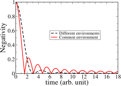
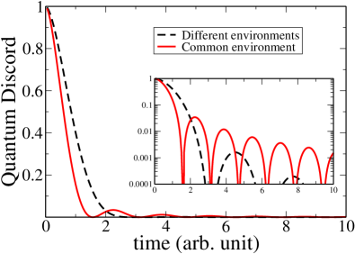
Figure 1: Time evolution of negativity (left panel) and QD (right panel) for two qubits subject to a static noise for different and common environments. To highlight the revivals of QD, its behavior is reported also in logarithmic scale in the inset of the right panel.

3.2 Random telegraph noise

For the case of a RTN affecting the dynamics of two qubits, the time evolution of the mixed state is evaluated from the average over the random phase factor $\varphi(t)$. After a straightforward calculation, we obtain

$$\rho_{de(ce)}(t)=\frac{1}{4}\left(\begin{array}[]{cccc}1+\Lambda_{de(ce)}&0&0&1+\Lambda_{de(ce)}\\ 0&1-\Lambda_{de(ce)}&1-\Lambda_{de(ce)}&0\\ 0&1-\Lambda_{de(ce)}&1-\Lambda_{de(ce)}&0\\ 1+\Lambda_{de(ce)}&0&0&1+\Lambda_{de(ce)}\end{array}\right),$$ (13)

with $\Lambda_{de}$=$D_{2\nu}^{2}(t)$ and $\Lambda_{ce}$=$D_{4\nu}(t)$. As shown elsewhere [29], the function $D(t)$ corresponds to the average phase factor $\langle e^{i\varphi(t)}\rangle$ and can be expressed as

$$D_{m\nu}(t)=\left\{\begin{array}[]{ccc}e^{-\gamma t}\left[\cosh{\left(\delta_{m\nu}t\right)}+\frac{\gamma}{\delta_{m\nu}}\sinh{\left(\delta_{m\nu}t\right)}\right]&\quad\textrm{for}&\gamma>m\nu\\ e^{-\gamma t}\left[\cos{\left(\delta_{m\nu}t\right)}+\frac{\gamma}{\delta_{m\nu}}\sin{\left(\delta_{m\nu}t\right)}\right]&\quad\textrm{for}&\gamma<m\nu\end{array}\right.,$$ (14)

where $\delta_{m\nu}$=$\sqrt{|\gamma^{2}-(m\nu)^{2}|}$ with $m\in\{2,4\}$. Unlike the static noise, the two-qubit density matrix assumes an X form both for different and common environment at any time $t$. It is worth noting that, for both RTN configurations, the long time asymptotic form of the states obtained is the same found for the static noise. Using again the definition of Eq. (7), negativity reads:

$$\mathcal{N}_{de}(t)=D_{2\nu}^{2}(t)\quad\textrm{and}\quad\mathcal{N}_{ce}(t)=|D_{4\nu}(t)|.$$ (15)

In this case, due to the X form of the states, it is possible to give the analytical expressions for QD by following the Luo approach [31]. They read:

$$\mathcal{Q}_{de}(t) = \frac{1}{2}\left[(1+D_{2\nu}^{2})\log_{2}{\left(1+D_{2\nu}^{2}\right)}+(1-D_{2\nu}^{2})\log_{2}{\left(1-D_{2\nu}^{2}\right)}\right]$$

$$\mathcal{Q}_{ce}(t) = \frac{1}{2}\left[(1+D_{4\nu})\log_{2}{\left(1+D_{4\nu}\right)}+(1-D_{4\nu})\log_{2}{\left(1-D_{4\nu}\right)}\right].$$ (16)

The dynamics of $\mathcal{N}$ and $\mathcal{Q}$ is shown in Fig. 2. In agreement with the outcomes of previous works [28], in the Markovian regime both entanglement and QD exhibits an exponential decay with time. On the other hand, in the non-Markovian regime the amount of quantum correlation are a damped oscillating function of time, thus displaying sudden death and revival phenomena. Finally, it should be noticed that our calculations show that, in the Markovian regime, the quantum correlations for the case of coupling of two qubits with the common environment are weaker with respect to the case of local qubit-environment interaction. Such a behavior is in contrast with the one found for non-Markovian noises and can be ascribed to the fact that indirect qubit-qubit interaction is here more effective in destroying both entanglement and QD.

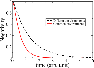
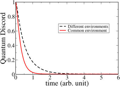
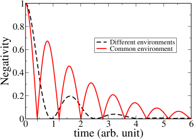
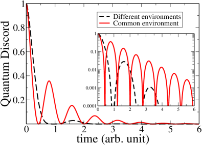
Figure 2: Top panels: Time evolution of negativity (left) and QD (right) for two qubits subject to a RTN for different and common environments when $\nu/\gamma=0.2$ (Markovian regime). Bottom panels: Time evolution of negativity (left) and QD (right) for two qubits subject to a RTN for different and common environments when $\nu/\gamma=5$ (non-Markovian regime). To highlight the revivals of QD, its behavior is reported also in logarithmic scale in the inset of the right panel.

4 Conclusions

In this paper we have analyzed the effects of both independent and common noisy environments on the dynamics of quantum correlations of two non-interacting qubits. Negativity and QD have been computed, using both analytical and numerical techniques. Static and slow RTN are classified as non-Markovian noises, while the fast RTN mimics a Markovian environment. We showed that, starting from a maximally entangled state, the quantum correlations display different decaying behaviors, depending on the nature of the considered noise. In particular, Markovian environments lead to a monotonic decay, while in non-Markov regimes sudden death and revival phenomena are present, in agreement with previous results in the literature[20, 32]. Specifically, here we ascribe the decay of revivals obtained in the static noise to the continuous nature of the random noise parameter. In fact our analysis clearly shows the suppression of quantum correlations at long times unlike previous investigations where an environmental noise mimicked by means of dichotomic time-independent noise parameter leads to non decaying entanglement revivals[21].
For both static noise and slow RTN, our results highlight that a common environment preserves better quantum correlations. It is worth noting that the opposite is found for qubits subject to a fast RTN, where the effect of a common noise results in a faster decay of correlations with respect to the case of independent environments.

An interesting generalization of our model is the possibility to sum up many RTNs, each with a specific switching rate, in order to obtain $1/f^{\alpha}$ noise. This noise is ubiquitous in solid state devices[33] and can be simulated considering a linear superposition of different RTNs, with an appropriate distribution of their switching rates. Furthermore, our study of the effects of static and dynamic noise on the evolution of quantum correlations in two-qubit models, has a natural and quite promising generalization in the case of systems with a larger number of degrees of freedom. For instance the model here studied can be used to extend, to the presence of noise, previous works on quantum walks on a one-dimensional lattice[34]. In this case the environmental noise would be a consequence of the lattice disorder. Work along these lines is in progress and results will be reported elsewhere.

Appendix A Explicit derivation of the two-qubit density matrix

Given the Hamiltonian in Eqs. (1) and (2), the associated evolution operator reads:

$$U_{de(ce)}= e^{-2i\beta t}\left(\begin{array}[]{cccc}A_{de(ce)}&-iB_{de(ce)}&-iC_{de(ce)}&-D_{de(ce)}\\ -iB_{de(ce)}&A_{de(ce)}&-D_{de(ce)}&-iC_{de(ce)}\\ -iC_{de(ce)}&-D_{de(ce)}&A_{de(ce)}&-iB_{de(ce)}\\ -D_{de(ce)}&-iC_{de(ce)}&-iB_{de(ce)}&A_{de(ce)}\end{array}\right),$$ (21)

where

$$A_{de}=\cos(\varphi_{A}(t))\cos(\varphi_{B}(t))\quad\quad A_{ce}=\cos^{2}(\varphi(t))$$

$$B_{de}=\cos(\varphi_{A}(t))\sin(\varphi_{B}(t))\quad\quad B_{ce}=\cos(\varphi(t))\sin(\varphi(t))$$

$$C_{de}=\sin(\varphi_{A}(t))\cos(\varphi_{B}(t))\quad\quad C_{ce}=B_{ce}=\cos(\varphi(t))\sin(\varphi(t))$$

$$D_{de}=\sin(\varphi_{A}(t))\sin(\varphi_{B}(t))\quad\quad D_{ce}=\sin^{2}(\varphi(t)),$$

with the phase $\varphi(t)=ct$ in the case of static noise and $\varphi(t)=-\nu\int_{0}^{t}c(t^{\prime})dt^{\prime}$ for the RTN. Applying the evolution operator to the initial state $\rho_{0}=|\Phi^{+}\rangle\langle\Phi^{+}|$, it is possible to obtain the time-evolved density matrix of the system corresponding to a specific choice of the random parameter:

$$\rho(\varphi,t)=U_{de(ce)}^{+}\rho_{0}U_{de(ce)}^{\dagger}=$$

$$=\frac{1}{2}\left(\begin{array}[]{cccc}\tilde{A}_{de(ce)}&\tilde{B}_{de(ce)}&\tilde{B}_{de(ce)}&\tilde{A}_{de(ce)}\\ -\tilde{B}_{de(ce)}&\tilde{C}_{de(ce)}&\tilde{C}_{de(ce)}&-\tilde{B}_{de(ce)}\\ -\tilde{B}_{de(ce)}&\tilde{C}_{de(ce)}&\tilde{C}_{de(ce)}&-\tilde{B}_{de(ce)}\\ \tilde{A}_{de(ce)}&\tilde{B}_{de(ce)}&\tilde{B}_{de(ce)}&\tilde{A}_{de(ce)}\end{array}\right)$$ (26)

where:

$$\tilde{A}_{de(ce)}=(A_{de(ce)}-D_{de(ce)})^{2}$$

$$\tilde{B}_{de(ce)}=i(B_{de(ce)}+C_{de(ce)})(A_{de(ce)}-D_{de(ce)})$$ (27)

$$\tilde{C}_{de(ce)}=(B_{de(ce)}+C_{de(ce)})^{2}$$

The average of the expression 26 over the possible values of the noise parameters gives the state of the system at time $t$ and corresponds to the integral

$$\langle\dots\rangle_{\varphi}=\int d\varphi(\dots)p(\varphi,t)$$ (28)

where for the static noise the phase distribution $p(\varphi,t)=P(c)/t$ where $P(c)$ is the flat distribution given in Sec. 2.1, while for the RTN, it takes the form[35]:

$$p(\varphi,t) =\frac{1}{2}e^{-\gamma t}\left\{[\delta(\varphi+\nu t)+\delta(\varphi-\nu t)]+\frac{\gamma}{\nu}[\Theta(\varphi+\nu t)+\Theta(\varphi-\nu t)]\right\}$$

$$\times\left[\frac{I_{1}\left(\gamma t\sqrt{1-(\varphi/\nu t)^{2}}\right)}{\sqrt{1-(\varphi/\nu t)^{2}}}+I_{0}\left(\gamma t\sqrt{1-(\varphi/\nu t)^{2}}\right)\right].$$ (29)

$I_{k}(x)$ is the modified Bessel function and $\Theta(x)$ is the Heaviside step function. After performing the integration, the average density matrices take the form of Eqs. (11) and (13) for the static noise and the RTN respectively.

References

- [1] C.H. Bennet and S.J. Wiesner, Phys. Rev. Lett. 69 (1992) 2881.
- [2] P. Shor, SIAM J. Computing 26 (1997) 1484.
- [3] S. Maniscalco, S. Olivares, M. G. A. Paris, Phys. Rev. A 75, 062119 (2007); R. Vasile, S. Olivares, M. G. A. Paris, S. Maniscalco, Phys. Rev. A 80, 062324 (2009).
- [4] R. Vasile, S. Olivares, P. Giorda, M. G. A. Paris, S.Maniscalco, Phys. Rev. A 82, 012312 (2010).
- [5] R. Vasile, S. Olivares, M. G. A. Paris, S. Maniscalco Phys. Rev. A 83, 042321 (2011).
- [6] M. Genoni, P. Giorda, M. G. A. Paris, Phys. Rev. A 78, 032303 (2008); G. Brida, I. Degiovanni, A. Florio, M. Genovese, P. Giorda, A. Meda, M. G. Paris, A. Shurupov, Phys. Rev. Lett. 104, 100501 (2010).
- [7] F. Buscemi, P. Bordone, and A. Bertoni, Phys. Rev. B 81 (2010) 045312.
- [8] F. Buscemi, P. Bordone, and A. Bertoni, New J. Phys. 13 (2011) 013023.
- [9] H. Ollivier and W.H. Zurek, Phys. Rev. Lett. 88 (2001) 017901.
- [10] L. Henderson, V. Vedral, J. Phys. A 34, 6899 (2001).
- [11] M. D. Lang, A. Shaji, C. M. Caves, Int. J. Quant. Inf. 9, 1553 (2011).
- [12] J. Maziero, L.C. Céleri, R.M. Serra, and V. Vedral, Phys. Rev. A 80 (2009) 044102.
- [13] T. Werlag, S. Souza, F.F. Fanchini, and C.J. Villas Boas, Phys. Rev. A 80 (2009) 024103.
- [14] T. Yu and J.H. Eberly, Science 323 (2009) 598.
- [15] T. Yu and J.H. Eberly, Phys. Rev. Lett. 93 (2004) 140404.
- [16] B. Bellomo, R. Lo Franco, and G. Compagno, Phys. Rev. Lett. 99 (2007) 160502.
- [17] Z. Ficek and R. Tanas, Phys. Rev. A 74 (2006) 024304.
- [18] L. Mazzola, S. Maniscalco, J. Piilo, K.A. Suominen, and B.M. Garraway, Phys. Rev. A 79 (2009) 042302.
- [19] A. W. Chin, S. F. Huelga, M. B. Plenio, arXiv:1103.1219.
- [20] D. Zhou, A. Lang, and R. Joynt, Quant. Inf. Comp. 9 (2010) 727.
- [21] R. Lo Franco, B. Bellomo, E. Andersson, and G. Compagno, Phys. Rev. A 85 (2012) 032318.
- [22] Y. Lahini, Y. Bromberg, D.N. Christodoulides, and Y. Silberberg, Phys. Rev. Lett. 105 (2010) 163905.
- [23] C. Thompson, G. Vemuri, and G.S. Agarwal, Phys. Rev. A 82 (2010) 053805.
- [24] T. Fujisawa and Y. Hirayama, Appl. Phys. Lett. 77 (2000) 543.
- [25] C. Kurdak, C.-J. Chen, D. C. Tsui, S. Parihar, S. Lyon, and G. W. Weimann, Phys. Rev. B 56 (1997) 9813.
- [26] G. Falci, A. D’Arrigo, A. Mastellone, and E. Paladino , Phys. Rev. Lett. 94 (2005) 167002.
- [27] E. Paladino, L. Faoro, G. Falci, and R. Fazio, Phys. Rev. Lett. 88 (2002) 228304.
- [28] P. Bordone, F. Buscemi, and C. Benedetti, Fluct. Noise Lett. 11 (2012) 1242003.
- [29] B. Abel, and F. Marquardt, Phys. Rev. B 78 (2008) 201302(R).
- [30] G. Vidal, and R.F. Werner, Phys. Rev. A 65 (2002) 032314.
- [31] S. Luo, Phys. Rev. A 77 (2008) 042303.
- [32] R Lo Franco, A D’Arrigo, G Falci, G Compagno and E Paladino, Phys. Scr. T147 (2012) 014019.
- [33] M.B. Weissman, Rev. Mod. Phys. 60 (1988) 537.
- [34] C. Benedetti, F. Buscemi, and P. Bordone, Phys. Rev. A 85 (2012) 042314.
- [35] J. Bergli, Y. M. Galperin and B. L. Altshuler, New J. Phys.11 025002.