The sub-mJy radio population of the E-CDFS: optical and infrared counterpart identification.

Abstract

We study a sample of 883 sources detected in a deep Very Large Array survey at 1.4 GHz in the Extended Chandra Deep Field South. The paper focuses on the identification of their optical and infrared (IR) counterparts. We use a likelihood ratio technique that is particularly useful when dealing with deep optical images to minimize the number of spurious associations. We find a reliable counterpart for 95% of our radio sources. Most of the counterparts (74%) are detected at optical wavelengths, but there is a significant fraction (21%) only detectable in the IR. Combining newly acquired optical spectra with data from the literature we are able to assign a redshift to 81% of the identified radio sources (37% spectroscopic). We also investigate the X-ray properties of the radio sources using the Chandra 4 Ms and 250 ks observations. In particular, we use a stacking technique to derive the average properties of radio objects undetected in the Chandra images. The results of our analysis are collected in a new catalog containing the position of the optical/IR counterpart, the redshift information and the X-ray fluxes. It is the deepest multi-wavelength catalog of radio sources, which will be used for future study of this galaxy population.

1. Introduction

Deep radio observations provide a powerful opportunity to investigate the high redshift Universe. Moreover, since radio observations are almost unaffected by dust extinction, they allow us to observe objects, which are heavily obscured in other bands. While bright radio sources are mostly powerful radio galaxies and radio-loud (RL) active galactic nuclei (AGN), at lower flux densities we observe an increasing fraction of star-forming galaxies (SFG) and radio-quiet (RQ) AGN (e.g., Padovani et al., 2009, and references therein).

Source classification of deep radio surveys is not easy and requires multi-frequency data. This approach was adopted in a series of papers, which studied a radio selected sample of 266 objects in the Chandra Deep Field South (CDFS; Kellermann et al., 2008; Mainieri et al., 2008; Tozzi et al., 2009; Padovani et al., 2009, 2011). Combining the information from different wavelengths, these authors were able first to classify the sources as SFG, RQ AGN and RL AGN and then to study the properties and the evolution of the different classes separately. The promising results of this work have encouraged us to apply it to a new radio catalog (N. Miller et al. 2012, in preparation) that reaches a lower flux density limit and has a more uniform coverage of the Extended-CDFS (E-CDFS). As a consequence, we have three times more objects, with most of the new sources in the sub-mJy regime (at 1.4 GHz).

This paper focuses on the identification of the optical and IR counterparts of the radio sources. Our main goal is to assign a redshift to the radio sources and to associate them with the correct photometry. This information will be then used in future papers to classify the sources and study their evolutionary properties. As mentioned above, a faint radio selected sample includes sources of widely different nature: SFG with a blue stellar population together with radio galaxies commonly hosted in redder objects, and obscured AGN together with bright unobscured quasars. For this reason, it is important to consider a large wavelength range, from the ultraviolet to the mid-infrared (MIR). Faint radio sources often correspond to faint optical counterparts. Therefore, deep optical observations are needed. This has an impact on the methodology that should be adopted in the identification process.

The structure of the paper is as follows: in Section 2 we present the datasets, while in Section 3 we describe the likelihood ratio method we used to identify the counterparts of our sources and the results of the identification process, including an estimate of the spurious association fraction and a comparison with the cross-correlation method. Section 4 discusses the redshift distribution (spectroscopic and photometric) of our sample. In Section 5 we deal with the X-ray counterparts of the radio sources, while the description of the released catalog is given in Section 6. In Section 7 we discuss our results and report our conclusions. Finally, in Appendix A we present new redshifts and spectra for the optical counterparts of 13 Very Large Array (VLA) sources and in Appendix B we report on some peculiar sources. In this paper we use magnitudes in the AB system, if not otherwise stated, and we assume a cosmology with $H_{0}=70$ km s^-1 Mpc^-1, $\Omega_{M}=0.3$ and $\Omega_{\Lambda}=0.7$.

2. Data

2.1. The radio catalog

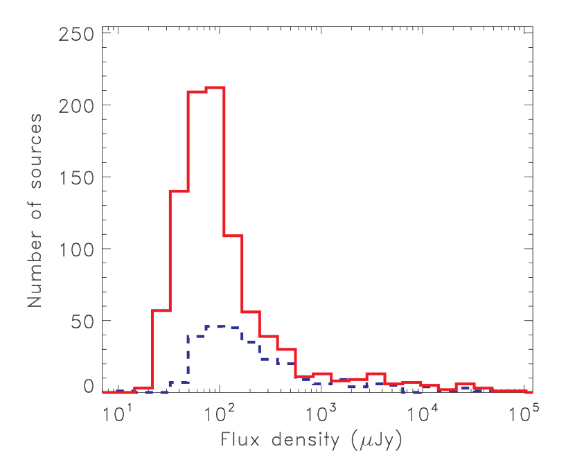
Figure 1.— Flux density distribution of the 5$\sigma$ E-CDFS radio catalog (solid line) compared to the sample described in Kellermann et al. (2008) (dashed line). The 5$\sigma$ sample is about three times larger and the majority of the sources have sub-mJy flux densities.

The E-CDFS was observed at 1.4 GHz with the VLA between 2007 June and September (Miller et al., 2008). The mosaic image covers an area of about $34\times 34$ arcmin with near-uniform sensitivity. The typical rms is 7.4 $\mu$Jy for a 2.8$\arcsec\times 1.6\arcsec$ beam. The second data release (N. Miller et al. 2012, in preparation) provides a new source catalog with a 5$\sigma$ point-source detection limit, for a total of 883 sources. We assigned a progressive identification number (RID) to the sources ordered by increasing right ascension. The flux density distribution of the sample is shown in Fig. 1, where we use the peak flux density or the integrated flux density according to the specifications of N. Miller et al. (2012, in preparation). The median value of the distribution is 58.5 $\mu$Jy and the median signal to noise ratio (S/N) is 7.6. We note that $\sim 90\%$ of the sample has flux density below 1 mJy, a regime where RQ AGN and SFG become the dominant populations (e.g., Padovani et al. 2009, 2011). A classification of the radio sources will be presented in M. Bonzini et al. (2012, in preparation).

2.2. Auxiliary data

The E-CDFS is one of the most studied patches of the sky and has been observed in many wavebands. As we will discuss in the following sections, this wealth of data is crucial to select the correct counterpart of a radio source. Here we describe the large amount of optical and IR data used in this work. We considered a total of ten catalogs. The complete list is reported in Table 1 together with some basic information: the instrument used (column 2), the effective wavelength (column 3), the typical point spread function (PSF) (column 4), the 5$\sigma$ AB magnitude limit (column 5), and the total area covered (column 6). The latter is also shown in Fig. 2, where the footprint of each mosaic image is plotted over the VLA image. For details on the different data sets, we refer to the papers listed in column 7. We divide the auxiliary catalogs in three groups according to their selection band: optical, near-infrared (NIR) and mid-infrared (MIR). The first group includes U-VIMOS, v-GEMS, R-WFI, and z-GOODS. We note that the Wide Field Imager (WFI) observations are the only optical images covering the whole VLA area. Therefore, even if they are shallower than the others and with a lower spatial resolution, they were crucial in the identification process. The U-VIMOS catalog has been produced by us using the SExtractor software (Bertin & Arnouts, 1996) from the original images. In the NIR, we used the H-GNS, H-SOFI, Ks-MUSYC and Ks-ISAAC catalogs. The H-GNS data, consisting of 30 pointed observations, cover a very small area of the E-CDFS but have a better resolution compared to the ground-based observations. At longer wavelengths, the E-CDFS was mapped with the Spitzer Space Telescope as part of the SIMPLE and FIDEL surveys. These data are particularly useful to identify high redshift sources (see Sec. 4.4 for details).

Table 1Auxiliary catalogs used for the identification of the radio sources counterparts. A description of the columns is given in Section 2.2.

	(1)	(2)	(3)	(4)	(5)	(6)	(7)
	Cataloga	Instrument	$\lambda_{eff}$ b	PSF FWHM	AB mag	Area	References
			($\mu$m)	(arcsec)	(5$\sigma$ limit)	(arcmin2)
Optical	U-VIMOS	VIMOS/ESO VLT	0.390	0.2	28.0	$\sim$800	Nonino et al. (2009)
	v-GEMS	ACS/HST	0.578	0.1	28.5	$\sim$800	Rix et al. (2004)
							Caldwell et al. (2008)
	R-WFI	WFI/ESO 2.2m	0.654	0.8	25.5	$>$1100	Giavalisco et al. (2004)
	z-GOODS	ACS/HST	0.912	0.1	28.2	$\sim$160	Dickinson et al. (2003)
							Giavalisco et al. (2004)
NIR	H-GNS	NICMOS/HST	1.607	0.2	26.5	$\sim$43	Conselice et al. (2011)
	H-SOFI	SOFI/ESO NTT	1.636	0.55	22.0	$\sim$800	Olsen et al. (2006)
	Ks-ISAAC	ISAAC/ESO VLT	2.745	0.4	24.7	$\sim$131	Retzlaff et al. (2010)
	Ks-MUSYC	ISPI/CTIO 4m	3.323	0.3	22.3	$\sim$900	Taylor et al. (2009)
MIR	IRAC-SIMPLE	IRAC/Spitzer	3.507-4.436c	1.7	23.8-23.6	$>$1100	Damen et al. (2011)
	24um-FIDEL	MIPS/Spitzer	23.209	6	20.2	$>$1100	Dickinson & FIDEL team (2007)

^a Name used in the text to refer to a specific catalog.
^b Filter effective wavelength.
^c The catalog is obtained from a combined image of 3.6$\mu$m and 4.5$\mu$m IRAC bands.

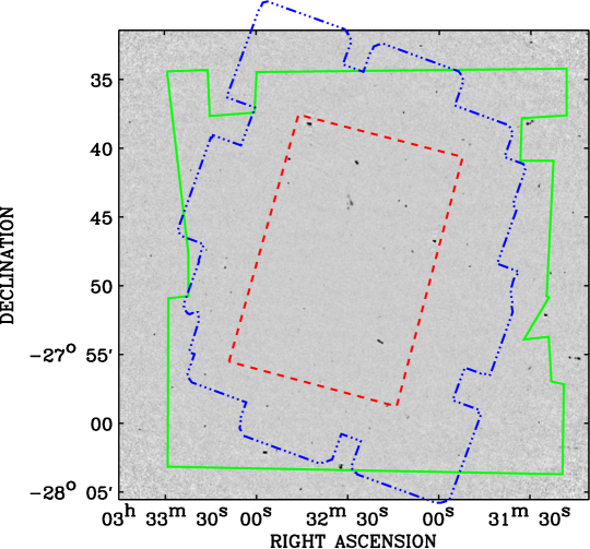
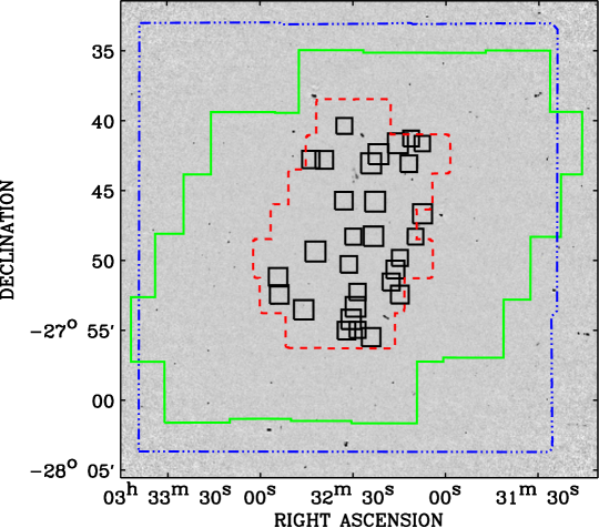
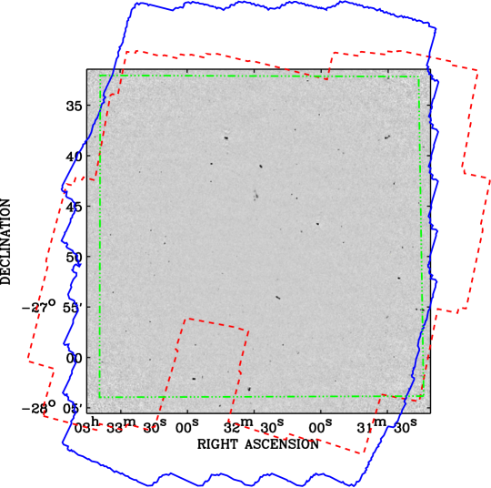
Figure 2.— Multi-wavelength coverages overplotted on the VLA image. Left: Optical catalogs (from outside): v-GEMS (solid line), U-VIMOS (dot-dashed line), and z-GOODS (dashed line). The R-WFI catalog coverage exceeds the VLA image and therefore is not plotted. Middle: NIR catalogs (from outside): Ks-MUSYC (dot-dashed line), H-SOFI (solid line), Ks-ISAAC (dashed line) and H-GNS (small squares). Right: MIR catalogs: IRAC-SIMPLE (dashed line) and 24um-FIDEL (solid line). The dot-dashed line encloses the area with photometric redshift catalogs coverage (see Section 4).

3. Counterpart identification method

3.1. Likelihood ratio technique

The first step in the identification process consisted of registering each auxiliary catalog to the astrometric frame of the radio image, correcting for the median offsets between the radio and the auxiliary catalogs. An average number of 400 sources was used to perform this registration and the typical median offset is 0.2$\arcsec$. As already mentioned, a simple cross-correlation method, where the counterpart is selected as the closest object to the radio source given a threshold matching radius, can lead to a large number of spurious association when dealing with deep optical images. Therefore, we adopted a likelihood ratio technique (e.g., Sutherland & Saunders, 1992; Ciliegi et al., 2003). This method allows us to take into account not only the position of the counterpart, but also the background source magnitude distribution and the presence of multiple possible counterparts for the same radio source. Here we briefly describe this technique following the formalism described in Ciliegi et al. (2003). It consists of three main steps:

1. Compute the surface density of background sources $n(m)$ as a function of magnitude $m$.

2. Evaluate the likelihood ratio ($LR$) for each possible counterpart.

3. Compute the reliability ($rel$) of each association.

(a) The magnitude distribution of background sources is obtained by counting all the sources within a 30$\arcsec$ radius around each radio object and dividing them in magnitude bins ($\Delta m=0.5$). The size of the searching radius is set to contain, on average, just one radio source and a substantial number ($>$100) of background sources for the deep optical catalogs. The surface density of background objects $n(m)$ is then computed dividing the obtained distribution by the total searching area ($\pi\times(30\arcsec)^{2}\times N_{radio\ sources}$).

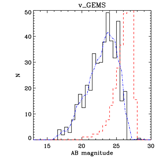
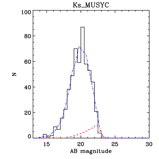
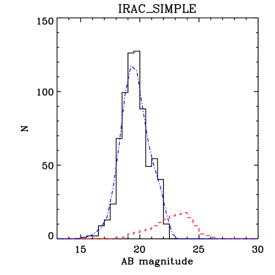
Figure 3.— Background source distribution, $n(m)$, multiplied for the searching area ($\pi\times(2\arcsec)^{2}\times N_{radio\ sources}$) (dashed line) and the background subtracted distribution of counterparts, $real(m)$, (solid line) for the v-GEMS catalog (on the left), the Ks-MUSYC catalog (in the middle) and the IRAC-SIMPLE catalog (on the right). The dotted dashed line is obtained by smoothing the $real(m)$ distribution and it is used to compute $q(m)$.

(b) The likelihood ratio for a counterpart candidate is defined as the ratio between the probability that the source is the correct identification and the corresponding probability for an unrelated background source. Therefore we compute $LR$ as:

$$LR=\frac{q(m)f(r)}{n(m)}$$ (1)

where $f(r)$ is the probability distribution function of the positional errors and $q(m)$ is the expected distribution of the counterparts as a function of $m$. As for $f(r)$ we adopt a two-dimensional Gaussian distribution of the form:

$$f(r)=\frac{1}{2\pi\sigma}\exp{(\frac{-r^{2}}{2\sigma^{2}})}$$ (2)

where $\sigma$ is the average between $\sigma_{x}=\sqrt{er^{2}_{aux}+er^{2}_{\alpha}}$ and $\sigma_{y}=\sqrt{er^{2}_{aux}+er^{2}_{\delta}}$. $\ er_{\alpha}$ and $er_{\delta}$ are the radio positional errors given by the beam size ($1.6\times 2.8$ arcsec) divided by two times the S/N ratio of the considered source. To account for further uncertainties on the VLA position, we added in quadrature 0.1$\arcsec$ to the radio positional error (N. Miller et al., 2012, in preparation). The average positional error $er_{aux}$ for the optical catalog is $0.1\arcsec$ and 0.3$\arcsec$ for the others, with the exception of H-GNS ($er_{aux}=0.2\arcsec$) and 24$\mu$m-FIDEL ($er_{aux}=0.6\arcsec$) (see references given in Table 1). To derive an estimate for $q(m)$, we first counted all the objects in the auxiliary catalog within a radius of 2$\arcsec$ around each radio source. Then, we subtracted the distribution of background objects computed on the same area ($n(m)\times\pi\times(2$”$)^{2}\times N_{radio\ sources}$). The latter is shown in Fig. 3 (dashed line), from left to right, for an optical, NIR and MIR catalog, respectively. The background subtracted distribution, $real(m)$, is plotted in the same figure as a solid line. Finally, we normalized the distribution function as:

$$q(m)=\frac{real(m)}{\sum_{i}real(m)_{i}}\times Q$$ (3)

where the sum runs over the total number of objects in the $real(m)$ and $Q$ represents the probability that the real counterpart is above the catalog detection limit. As already verified by Ciliegi et al. (2003) and Mainieri et al. (2008), the number of identifications and the associated reliabilities have a mild dependence on $Q$. Therefore, we adopted a fixed value $Q=0.8$ for all the auxiliary catalogs as it corresponds to the average expected fraction of identifications. Finally, combining $q(m)$, $f(r)$ and $n(m)$ according to eq. 1, we computed the LR for each source in the auxiliary catalogs.

(c) The LR does not contain information about the possible presence of many counterpart candidates in the surrounding of a specific radio source. It is therefore useful to define the reliability of each association as:

$$rel_{j}=\frac{(LR)_{j}}{\sum_{i}(LR)_{i}+(1-Q)}$$ (4)

where the sum is over all the candidate counterparts for the same radio source (Sutherland & Saunders, 1992).

3.2. Identification results

Following the method described in the previous section, we built a list of possible counterparts for each auxiliary catalog. Initially, we set a very low likelihood threshold ($10^{-6}$) to be sure not to lose any counterpart. After a careful analysis, we decided to consider as reliable only counterparts with reliability greater than 0.6. This threshold ensures that the expected number of spurious associations is below 5% for each auxiliary catalog (see Section 3.5), and at the same time maximizes the number of identified sources. The identification rate for each auxiliary catalog is reported in column (3) of Table 2. The number of identified sources is weighted by the number of radio sources inside the area covered by each survey reported in column (2). We note that the number of identifications increases with wavelength, from $\sim 65\%$ in the optical catalogs up to $87\%$ in the MIR. That means that most of the radio sources have a counterpart candidate in more than one auxiliary catalog, and that there is a fraction of sources that are not detected in the optical but only in the IR. In more detail, there are 652 radio sources (74%) that have a counterpart in at least one of the four optical catalogs, 76 (9%) that have no counterpart in any of the optical catalogs, but that are identified in at least one of the NIR catalogs, and 111 (12%) that have a counterpart only in the MIR. We will refer to these three groups as optical, NIR and MIR selected counterparts, respectively. We anticipate that they have different redshift distributions, with NIR and MIR selected sources having on average higher redshift (see Section 4.4). High redshift objects, thanks to their positive K-correction, are more easily observed in the IR than in the optical and this explains the higher identification rate observed in the MIR catalogs.

Table 2Counterparts identified in each catalog and spurious association estimate for both the likelihood and cross-correlation methods. In column 2 we report the number of radio sources inside the area of the survey (see Fig. 2).

			LR method			cross-correlation
	(1)	(2)	(3)	(4)	(5)	(6)	(7)
	Catalog	Radio sources	% counterparts (#)	90% inside a	% spurious	% counterparts (#)	% spurious
				(arcsec)
Optical	U-VIMOS	540	64% (347)	0.7	5%	64% (346)	12%
	v-GEMS	646	67% (432)	0.7	5%	67% (435)	11%
	R-WFI	877	68% (600)	0.7	3%	67% (587)	6%
	z-GOODS	164	65% (107)	0.5	4%	58% (95)	6%
NIR	H-GNS	34	70% (24)	0.5	$<$1%	62% (21)	6%
	H-SOFI	523	69% (363)	0.7	2%	65% (339)	1%
	Ks-ISAAC	135	81% (109)	0.7	4%	76% (102)	3%
	Ks-MUSYC	724	77% (556)	0.7	3%	71% (515)	1%
MIR	IRAC-SIMPLE	858	87% (746)	0.7	3%	79% (674)	3%
	24um-FIDEL	878	85% (745)	1.1	4%	79% (692)	2%

^a Radius within 90% of the counterparts are included.

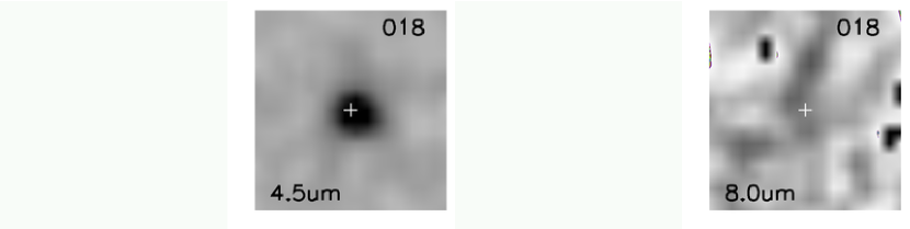
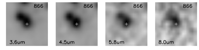
Figure 4.— Spitzer/IRAC images of objects RID 018 (top) and 866 (bottom). They represent examples of IRAC sources not present in the SIMPLE catalog whose position has been manually extracted (see Section 3.4 for details): RID 018 has been observed only in two of the four channels, and RID 866 is blended by a nearby source. The position of the radio source is marked by a cross. Each image is 10 arcsec on a side.

Table 3Radio information and identification process results. A description of the table content is given in Section 6. (This Table is available in its entirety in a machine-readable form in the online journal. A portion in shown here for guidance regarding its form and content.)

(1)	(2)	(3)	(4)		(5)	(6)	(7)	(8)	(9)	(10)
RID	RA radio	Dec radio	Sr		S/N	RA counterpart	Dec counterpart	Reliability	Distance	Counterpart
	(J2000)	(J2000)	($\mu$Jy)			(J2000)	(J200)		(arcsec)	catalog
360	3:32:13.09	-27:43:50.9	1380.0$\pm$	26.6	115.8	—	—	—	—	unidentified
361	3:32:13.24	-27:40:43.7	58.9$\pm$	6.4	9.0	03:32:13.24	-27:40:43.39	0.97	0.2	R-WFI
362	3:32:13.25	-27:42:41.3	86.4$\pm$	6.4	13.5	03:32:13.25	-27:42:40.86	1.00	0.2	z-GOODS
363	3:32:13.36	-27:39:35.2	48.5$\pm$	6.9	7.0	03:32:13.32	-27:39:35.03	1.00	0.2	24um-FIDEL
364	3:32:13.41	-27:33:04.9	48.4$\pm$	7.8	6.2	03:32:13.39	-27:33:04.93	0.97	0.3	R-WFI
365	3:32:13.50	-27:49:53.1	44.0$\pm$	6.4	6.9	03:32:13.48	-27:49:52.82	1.00	0.1	z-GOODS
366	3:32:13.61	-27:34:04.3	102.6$\pm$	18.5	8.3	03:32:13.58	-27:34:04.37	1.00	0.4	R-WFI
367	3:32:13.65	-28:01:01.2	35.7$\pm$	6.9	5.1	03:32:13.62	-28:01:01.06	1.00	0.3	v-GEMS
368	3:32:13.85	-27:56:00.3	44.5$\pm$	6.4	6.9	03:32:13.85	-27:55:59.95	1.00	0.2	24um-FIDEL
369	3:32:14.17	-27:49:10.6	95.4$\pm$	6.4	14.9	03:32:14.14	-27:49:10.09	0.98	0.4	U-VIMOS
370	3:32:14.46	-27:45:40.8	34.9$\pm$	6.2	5.6	03:32:14.43	-27:45:40.72	1.00	0.3	z-GOODS
371	3:32:14.60	-27:43:05.8	32.1$\pm$	6.4	5.0	03:32:14.60	-27:43:06.10	9.00	0.3	manual
372	3:32:14.69	-28:02:20.2	44.9$\pm$	7.1	6.0	03:32:14.65	-28:02:19.97	1.00	0.4	v-GEMS
373	3:32:14.85	-27:56:40.9	109.7$\pm$	6.5	16.9	03:32:14.83	-27:56:40.49	1.00	0.2	v-GEMS
374	3:32:15.17	-28:05:22.7	50.8$\pm$	7.9	6.3	03:32:15.14	-28:05:22.24	1.00	0.3	R-WFI
375	3:32:15.34	-27:50:37.6	43.1$\pm$	6.4	6.7	03:32:15.32	-27:50:37.25	1.00	0.1	H-GNS

In Table 3, we report the complete list of the counterparts of the radio sources (see Section 6). The counterpart position is taken from an optical catalog, when available, since these observations have the highest spatial resolution. In particular, we chose the catalog in which the counterpart has the highest reliability. According to this criterion, we selected 104 counterparts from U-VIMOS, 150 from v-GEMS, 301 from R-WFI, and 96 from z-GOODS. If there was no optical counterpart above the reliability threshold, we used the coordinates of the most reliable counterpart found in the NIR catalogs. This happened for 4 sources from H-GNS, 24 from H-SOFI, 4 from Ks-ISAAC, and 47 from Ks-MUSYC. For the remaining counterparts, we used the position from the IRAC-SIMPLE catalog (25 sources) and from the 24um-FIDEL one (74 sources). Finally, there are 10 radio sources (RID: 18, 19, 36, 371, 430, 457, 463, 698, 795, and 866) whose counterpart is clearly visible in the IRAC images but is not listed in the SIMPLE catalog (or in any other catalog). The reason is that, since the SIMPLE catalog is extracted from the combined 3.6 and 4.5 $\mu$m images, either the source was observed only in the first or the second IRAC channel and therefore not included in the catalog, or it was not deblended from a nearby object (see Fig. 4). In these cases we have extracted the position of the counterpart from the IRAC image.

As a further check, we extracted 10$\times$10 arcsec cutouts centered at the radio source position of the images in the various bands, to visually inspect the counterpart associations. Examples are presented in Fig. 5 where the position of the radio source and of its counterpart are marked by a cross and a square, respectively. In the left panels, radio contours are plotted over a 20$\times$20 arcsec R band image, after the latter has been registered on the astrometric frame of the radio image. This larger size is chosen for a better view of the radio contours. In most cases the selected counterpart is clearly visible in one or more cutouts. In 12 cases, we found a more convincing counterpart and therefore we revisited the association; these cases are discussed in more details in Section 3.4.

A total of 44 sources are unidentified: most of them are either very faint radio sources or lie at the edge of the field, where the multi-wavelength coverage is less rich. They are blank fields in all the available images (see, e.g., RID 360 in Fig. 5). We expect only few of them to be spurious radio detections since the radio catalog is based on a mosaic image and therefore each object was observed by more than one pointing (N. Miller et al., 2012, in preparation). If an object were spurious and due to instrumental effects (e.g., a sidelobe of a nearby bright source) it would not be the same in each pointing. Similarly, if it were just a chance noise spike you would expect to see it in only one pointing. Therefore we perform source fits in the individual pointings for the unidentified radio sources with low S/N and we believe that the radio detections are real, with one or two possible exceptions.

In summary, we found a reliable counterpart for 839 out of 883 radio sources (95%).

Figure 5.— Left panels: radio contours plotted over a 20$\times$20 arcsec R band image. The RID is shown on the top right of each image. Other panels: cutouts of the images in the various bands centered at the position of the radio source (marked by a cross). Each image is 10 arcsec on a side. The corresponding catalog is indicated on the bottom left. The square indicates the position of the selected counterpart. The image from which the counterpart is selected has a black border.

3.3. Multiple component radio systems

A multi-wavelength approach is crucial to identifying multiple-component systems. Indeed, the analysis of the radio morphology alone cannot distinguish between pairs of radio sources which are close in projection, or physically connected radio components of the same source. In our sample there are 24 systems, whose radio morphology can be interpreted as multi-component radio sources. Their radio contours are plotted over the R image in Fig. 6.

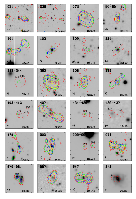
Figure 6.— Cutouts of radio sources with complex radio morphology. The majority of them ($17/24$) are confirmed as multiple-component system, while for the remaining we find reliable counterparts for each radio component (see Section 3.3 for details). Radio contours are plotted over the R band WFI image. The scale of the cutout is given in arcsec on the bottom right and the RID on the top left.

We perform the likelihood ratio analysis described in Section 3.1 to look for a possible counterpart of each single radio component. For seven such systems (panels (d), (i), (n), (o), (p), (s), (u) in Fig. 6), we find highly reliable counterparts for each component. Therefore, we claim that they represent distinct sources. The other 17 are confirmed to be multiple-component systems. They have extended radio emission, in most of the cases characterized by a core (not always visible in the radio) and radio lobes. The radio lobes have usually comparable radio power and are not associated with any optical or IR counterpart. There are some cases where we cannot exclude a possible contribution to the radio flux density from a superimposed unrelated object like in sources with RID 38, 73, 209, 283, and 647. The complete list of these system with the properties of each radio component is given in N. Miller et al. (2012, in preparation). In Appendix B we discuss some peculiar sources.

3.4. Revisited associations

In section 3.1, we described our method to select the optical and IR counterpart for the radio sources using a likelihood ratio technique. Visually inspecting the results of the identification process, we confirm the association obtained following this procedure in 99% of the cases. In this section, we describe the reasons why we revisited the counterpart association for some peculiar sources. In these cases, the most likely counterpart has a reliability under our threshold and was therefore rejected. The two main reasons for this are: (i) the radio source is in a crowded field and therefore all the possible counterparts have low reliability (RID 70, 407, 417, 458, 561, and 797). We based our choice of the counterpart on the radio morphology and on the overall object properties in the various bands (as an example, see the notes on RID 407 in Appendix B). (ii) The radio source is extended, hence the exact position of the radio emission is not well determined or does not correspond to the optical/IR peak emission (RID 407, 420, 521, 804, 828, and 830). As a consequence, there is an offset between the position of the radio source and the counterpart that has therefore a low reliability.

3.5. Estimation of spurious associations and comparison with the cross-correlation method

For each auxiliary catalog, we estimate the rate of spurious associations by randomly shifting the position of the radio sources and computing again the reliability for all the possible counterparts. We apply only shifts between 5 and 15 arcsec in order not to exceed the field coverage. We then compute the likelihood ratio value for each one of the shifted sources using equation 1, where $q(m)$ and $n(m)$ are the probability distributions derived for the original catalog (see Section 3.1). The same reliability threshold of 0.6 is adopted. The average fraction of false association over 50 different shifts is reported in Table 2 for each auxiliary catalog. We find spurious fractions from 3% up to 5% for the deep optical catalogs. In the case of H-GNS the fraction is very low but it could be underestimated due to the small area covered by this catalog and the consequent small statistics.

We compare these results with the number of spurious associations obtained using a simple cross-correlation method. The matching radius chosen for this test is equal to the radius which includes 90% of the counterparts identified with the likelihood-ratio method. These radii are listed in column (4) of Table 2. We find that the two methods identify a similar fraction of sources for the optical catalogs and a somewhat lower one for the IR catalogs. We estimate the fraction of spurious associations similar to what has been done for the likelihood method, namely shifting the radio catalog with respect to the auxiliary one. We used the same set of displacements as in the previous case. As shown in Table 2, our likelihood ratio technique is generally less affected by spurious contamination especially when applied to the deep optical catalogs. In particular, in the cases of the U-VIMOS and v-GEMS catalogs the spurious fraction exceeds 10% with the cross-correlation method. If we decrease the searching radius from 0.7 to 0.5 arcsec for all the optical catalogs, the fraction of false counterparts becomes lower (8%, 7%, 3%, for the U-VIMOS, v-GEMS and R-WFI catalogs, respectively), but we also miss a significant fraction of real identification (19%, 23% and 14%, respectively). For NIR and MIR catalogs, the two methods are almost equivalent. We obtain slightly higher fractions of fake associations with the likelihood ratio technique but with the cross-correlation method we miss a larger number of counterparts. This is mainly due to the lower source surface density with respect to the optical catalogs. We note that the shift-and-rematch method tends to overestimate the number of false matches as it ignores the fact that there are a large fraction of the sources that do have counterparts (see Broos et al., 2007, 2011; Xue et al., 2011, for details.). Our estimates should therefore be considered as upper limits. Since this effect is the same both for the likelihood and the cross-correlation method, it does not affect our conclusions. Finally, we assume that the fraction of spurious association in the final catalog is equal to the weighted average of the spurious fraction of each catalog, using the number of counterparts selected from each catalog as weight. We then expect at most 4% spurious counterparts.

3.6. Comparison with previous work

The brighter sources of the present catalog were already included in the radio catalog described in Kellermann et al. (2008). We have compared the counterparts found in Mainieri et al. (2008) (M08, hereafter) with those selected in this work for the sources in common. We find that in 90% of the cases the same counterpart is selected. For the remaining 10%, we select a different counterpart compared to M08. In most cases the counterparts were identified in the optical band by M08 while we find a more convincing counterpart in newly acquired MIR observations. For eight out of twelve objects that were unidentified or under the threshold in M08, we now have a reliable counterpart. One example is RID 625 (ID in the Kellermann et al. (2008) catalog KID=202) that was in an empty field in M08 while we identify it at 24 $\mu$m. The criteria to identify the best counterpart candidate of a radio source are slightly different between the two works. In M08 a likelihood ratio threshold of 0.2 was adopted, while we use a cut in reliability to take into account the presence of multiple counterpart candidates of the same radio source. Our reliability threshold of 0.6 is a bit more conservative (it correspond to a $LR$ threshold of $\sim 0.3$) and it is aimed at reducing the number of spurious identifications. Another difference between the two works is that in M08 the best counterpart was chosen according to an a priori ranking of the auxiliary catalogs. The priority was set according to the depth of the optical/NIR survey and to the wavelength. Given the larger number of auxiliary catalogs used in this work we use a different approach: between catalogs in the same wavelength range (optical, NIR and MIR), we select the counterpart with the highest reliability (see Section 3.1). This allows us to fully exploit the information given by the probability distributions obtained with the likelihood ratio technique. Moreover, we minimize the number of tentative associations selected in a high priority optical/NIR catalog yet with a reliability just above the threshold. As a consequence, with our new approach 90% of the counterparts have a reliability greater than 0.96, in contrast to 0.83 obtained in M08 (see Fig. 4 in M08). Moreover, we observe a significant decrease in the average separation between the radio source and its counterpart compared to M08. In this work, we find 90% of the counterparts within 0.7 arcsec around the radio position, which is about half of the radius found in M08 (see Fig. 7). This is partially due to the change in resolution of the two radio surveys (from 3.5$\arcsec\ \times 3.5\arcsec$ in Kellermann et al. (2008) to 2.8$\arcsec\ \times 1.6\arcsec$ in this work).

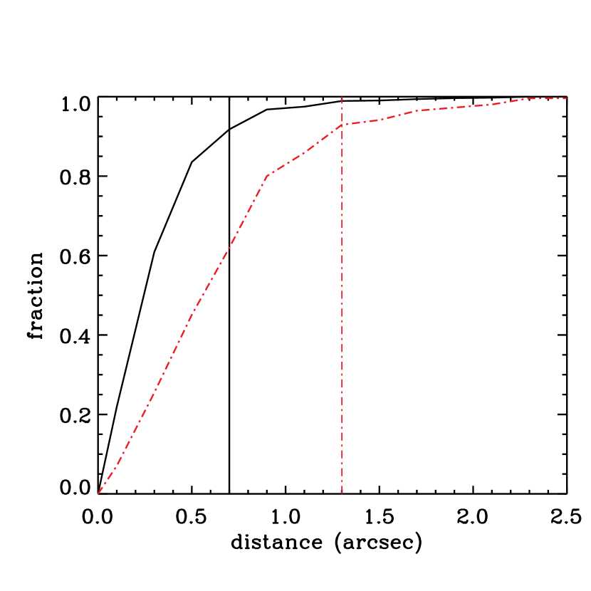
Figure 7.— Cumulative distribution of the separation between a radio source and its counterpart for the radio catalog presented in this work (solid line) and in Mainieri et al. (2008) (dot-dashed line). The vertical lines mark the separation within 90% of the counterparts are located.

In summary, using the new MIR imaging in the E-CDFS area, we reach the same fraction of identification (95%) as in M08, although we adopt a higher reliability threshold and a larger fraction of the radio sources is in the outer part of the field, where the multi-wavelength coverage is poorer. There is only one source previously identified that we now consider unidentified: RID 101 (see details in Appendix B).

Table 4List of the spectroscopic catalogs considered in this work. The instrument used to obtain the spectra is reported in column (2) and details on the observation and data reduction can be found in the references given in the first column. The label in column (3) are used in the final catalog to identify the source for the spectroscopic redshift. The last column reports the number of spectroscopic redshift adopted from each catalog in this work.

(1)	(2)	(3)	(4)
Reference	Instrument	Label	Number of z-spec adopted
This work	VIMOS	P81	13
Szokoly et al. (2004)	FORS1/FORS2	S04	38
Vanzella et al. (2008)	FORS2	FORS	20
Silverman et al. (2010)	VIMOS	VJB	37
Silverman et al. (2010)	VIMOS	P80	3
Silverman et al. (2010)	Keck	K07	32
Silverman et al. (2010)	Keck	K08	18
Treister et al. (2009)	VIMOS	T09	20
Balestra et al. (2010)	VIMOS-LR	VLR	24
Balestra et al. (2010)	VIMOS-MR	VMR	23
Le Fevre et al. (2004)	VIMOS	VVDS	19
Ravikumar et al. (2007)	VIMOS	R07	12
Szokoly et al. (2004)	FORS1/FORS2	S04F	1
J. Kurk et al., 2012 (Submitted)	FORS2	GMASS	4
Norris et al. (2006)	2dF	N06	10

4. Redshift associations

4.1. New VIMOS spectra and redshifts

We acquired new optical spectra with the Visible Multi-Object Spectrograph (VIMOS; Le Fèvre et al., 2003) at Very Large Telescope (VLT). We carried out one pointing in the central region of the VLA survey using the low-resolution (LR) blue grism (R=180, dispersion=5.7 Åpixel^-1) that covers the wavelength range 3700-6700 Å. The total exposure time of five hours was set to identify faint optical counterparts to a limiting point-source magnitude of R$\approx 25$. The mask was designed with the VIMOS Mask Preparation Software (VMMPS; Bottini et al., 2005) that optimizes the slit assignments based on our input catalog. We observed a total of 32 VLA sources. The data were reduced using the VIMOS Interactive Pipeline and Graphical Interface (VIPGI; Scodeggio et al., 2005), and the redshifts were estimated using the EZ software that cross-correlates each spectrum with a template spectrum, and via visual inspection to validate the result. We derived a spectroscopic redshift for 13 VLA sources for which previously we had only a photometric redshift estimate. The spectra of these 13 radio sources are shown in Appendix A.

4.2. Spectroscopic redshifts

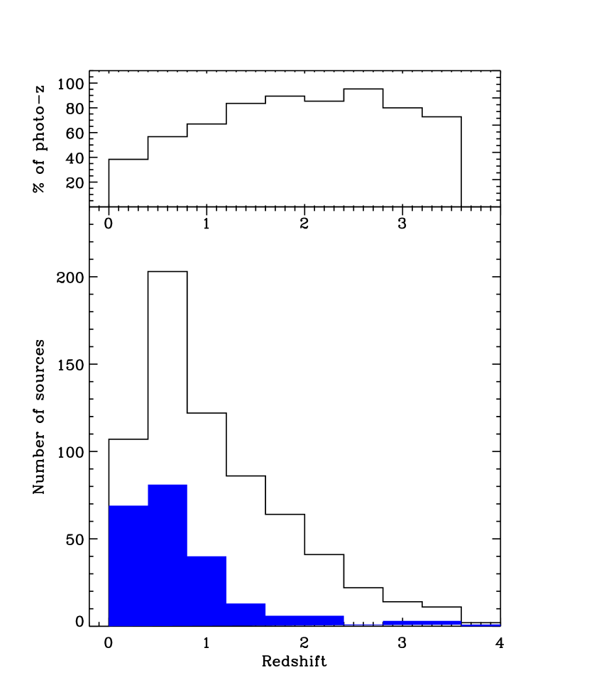
Figure 8.— Top panel: fraction of photometric redshifts as a function of redshift. Bottom panel: total (empty) and spectroscopic (filled) redshift distributions. The plot is cut at $z=4$ for a better view of the range where both photo-z and spec-z are available.

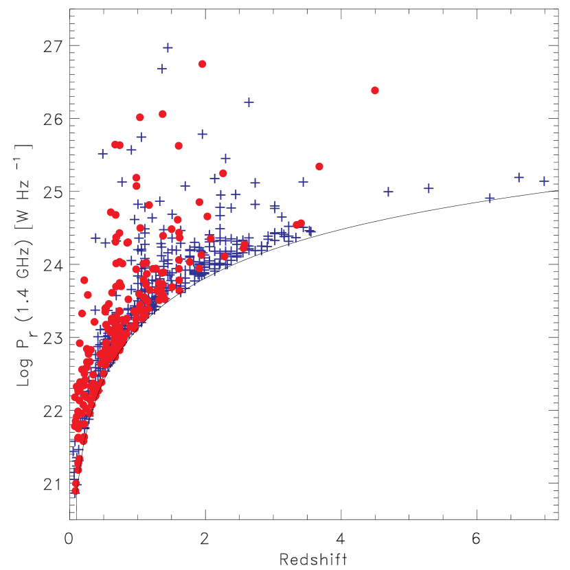
Figure 9.— Radio power as a function of redshift. Circles indicate spectroscopic redshifts while crosses indicate photometric redshifts. The solid line shows the radio flux density limit of the VLA survey.

Figure 10.— Normalized redshift distribution for the radio sources with an optical counterpart (top), with a NIR counterpart (middle) and with a MIR counterpart (bottom). The mean redshift is increasing from 1 for optical identified sources to 2.5 for the MIR ones (see Section 4.4).

Many spectroscopic campaigns have been conducted in the E-CDFS. A complete reference list for those used in this work can be found in Table 4. We combine the publicly available redshifts with our own newly acquired spectra (see Sec. 4.1). We assign a quality flag (QF) to each redshift by mapping the ones in the original catalogs to a uniform scale. We use QF=3 to indicate a secure redshift, QF=2 for reasonable redshift, and QF=1 for tentative redshift or for single line detection. The coordinates of the counterparts, identified as described in Sec. 3.1, are cross-correlated with the sources reported in the spectroscopic catalogs within 0.2 arcsec. Such a small radius is chosen to minimize the confusion with nearby sources. We find a spectroscopic redshift for 274 sources. If a source has a match in more than one spectroscopic catalog, we verify the consistency between the corresponding redshifts. For 22 sources, multiple spectroscopic redshifts differ by more than 0.1. In all but three of these cases, the QF of the spectroscopic measurements allows us to select the highest quality $z$. For sources RID= 83, 569, and 706, where the QF in the various spectroscopic catalogs are equivalent, we visually checked the spectra to select the more reliable redshift value. The spectroscopic redshift associated with each radio source is reported in the column 7 of Table 5, with the QF, and the reference in columns 8 and 9, respectively. In summary, 33% of the radio sources with counterpart have a spectroscopic redshift, 74% of which are secure redshift (QF=3), 18% have QF=2 and 8% have a tentative redshift measurement (QF=1).

4.3. Photometric redshifts

In order to increase the redshift completeness of our sample, we also use photometric redshift estimates. We use the photometric redshift catalog compiled by Luo et al. (2010) and Rafferty et al. (2011). These redshifts are based on a large number of photometric bands: the COMBO-17 optical catalog (Wolf et al., 2004; Wolf et al., 2008), the GOODS-S MUSIC catalog (Grazian et al., 2006), the MUSYC BVR-detected catalog (Gawiser et al., 2006), the deep GOODS-S VIMOS U-band catalog (Nonino et al., 2009), the GALEX Data Release 4, the MUSYC near-infrared catalogue (Taylor et al., 2009), and the SIMPLE mid-infrared one (Damen et al., 2011). Starting from this photometric data set, the publicly available Zurich Extragalactic Bayesian Redshift Analyzer (ZEBRA; Feldmann et al., 2006) code was used to derive photometric redshifts via a maximum likelihood technique. The set of templates used includes: 259 galaxy templates constructed from PEGASE stellar population synthesis models, a set of hybrid (galaxy+AGN) templates and ten empirical AGN templates from Polletta et al. (2007). We refer the reader to Luo et al. (2010) and Rafferty et al. (2011) for a more detailed description of the procedure adopted to estimate photometric redshifts. We cross-correlate the photometric redshift catalog with the radio source counterparts, selected as described in 3.2. Given the high background surface density distribution of the photometric catalog, we adopt a matching radius of 0.2 arcsec. This way we minimize the risk of associating to the radio counterpart the redshift of a nearby source. We find 623 matches out of the 839 identified radio sources. The mean separation between the radio counterparts and the corresponding photometric redshift coordinates is 0.03 arcsec. For the remaining 216 objects we consider three other compilations of photometric redshifts: the MUSYC-E-CDFS catalog (Cardamone et al., 2010), the GOODS-MUSIC catalog (Santini et al., 2009), and the K-selected MUSYC catalog (Taylor et al., 2009). The latter is based on a NIR selected catalog, and therefore is particularly useful to assign a redshift to radio sources with no counterpart in the optical. We find 13, 4, and 35 additional redshifts, respectively. In Summary, we associate a photometric redshift to 673 (80%) out of the 839 identified radio sources.

For the sub-sample with available secure spectroscopic redshift (QF=3), we compute the normalized median absolute scatter,

$$\sigma_{NMAD}=1.48\times median\left(\frac{|\Delta z-median(\Delta z)|}{1+z_{spec}}\right),$$ (5)

where $\Delta z=z_{phot}-z_{spec}$, which is an estimate of the quality of the photometric redshift which is less sensitive to outliers than the standard deviation (Brammer et al., 2008). We find $\sigma_{NMAD}=0.01$ that is comparable, and even slightly better, to what found for the same indicator in the photometric redshift catalogs considered (Santini et al., 2009; Taylor et al., 2009; Cardamone et al., 2010; Rafferty et al., 2011). Therefore, we conclude that the accuracy of the photometric redshifts for our radio selected sample is comparable to what estimated for the overall population in the photometric catalogs. We note that this indicator assumes that the spectroscopic sub-sample is representative of the full sample. This assumption is likely not entirely true and consequently it gives an overestimation of the accuracy of the photo-z for the whole sample. Luo et al. (2010) estimated that the uncertainties on the photometric redshifts for the full sample are a factor of six higher. We also note that the photometric redshift errors given in column 6 of Table 5 from the Rafferty et al. (2011) catalog are known to be underestimated (see Luo et al. (2010)). A more realistic estimate is given by the $\sigma_{NMAD}$ parameter, which is around 6% as discussed above.

4.4. Redshift distribution

In the case where both spectroscopic and photometric redshifts are available, we use the spectroscopic one if QF $\geq$ 2 and the photometric redshift otherwise. For spectroscopic redshifts with QF=1 we find $\sigma_{NMAD}=0.28$, which we interpret as an indication of the poor quality of these spectroscopic redshifts. Combining spectroscopic and photometric information, we assign a redshift to 678 objects, 81% of the radio sources with counterpart (252 spectroscopic redshifts and 426 photometric redshifts). This fraction underestimates the redshift completeness of our sample since in the outermost part of the field there are no redshift measurements available. Therefore, we restrict our redshift distribution analysis to the sources in the area covered by the photometric redshift catalogs. This region is plotted with a dot-dashed line in the right panel of Fig. 2. The number of radio sources included is 779, and 87% of them have a redshift. The total redshift distribution is plotted in Fig. 8, where the filled histogram represents the distribution of sources with spectroscopic redshifts. The top panel shows the fraction of photometric redshifts. We note that photometric redshift measurements become increasingly important at higher redshifts where optical spectroscopic observations become more challenging. The mean redshift for the whole sample is 1.1 and the median is 0.9. Fig. 9 shows the radio power as a function of redshift for sources with either spectroscopic (circle) or photometric (cross) redshift. The solid line represents the flux density limit of the survey. If we divide the radio sources based on their identification band, we observe an increase in the mean (median) redshift from 1.0 (0.8) for the optical identified sources to 2.5 (2.1) for the MIR ones (see Table 6 and Fig. 10). The statistical significance of the different redshift distributions is examined with the Kolmogorov-Smirnov (K-S) test. The difference between the optical and NIR distributions and that between the optical and MIR distributions are confirmed with a significance level $\gg 99\%$. For the NIR and MIR redshift distributions the K-S test gives a significance of 99%. Both spectroscopic and photometric redshift estimates become more challenging moving to high redshift objects and this is the reason why the fraction of sources with a redshift estimate drops from 88% for the optical identified sources to 25% for the MIR ones (see Table 6).

Table 5Main characteristics and redshift information of the radio source counterparts. A description of the table content is given in Section 6. (This table is available in its entirety in a machine-readable form in the online journal. A portion in shown here for guidance regarding its form and content.)

(1)	(2)	(3)	(4)	(5)	(6)	(7)	(8)	(9)	(10)	(11)	(13)
RID	R mag	Ks mag	3.6$\mu$m mag	best-z	photo-z	spec-z	QF	reference	S0.5-2keV	S2-10keV	XID
	(AB)	(AB)	(AB)						(erg cm-2 s-1)	(erg cm-2 s-1)
360	—	—	—	—	—	—	—	—	—	—	—
361	25.92 $\pm$ 0.22	22.02 $\pm$ 0.18	21.02 $\pm$ 0.02	1.39	$1.39^{+0.02}_{-0.18}$	—	—	—	—	—	—
362	20.40 $\pm$ 0.00	18.47 $\pm$ 0.01	18.46 $\pm$ 0.00	0.61	$0.60^{+0.00}_{-0.00}$	0.607	3	VMR	(1.58$\pm$0.04)$\times 10^{-15}$	(1.06$\pm$0.02$)\times 10^{-14}$	193
363	—	—	21.33 $\pm$ 0.30	—	—	—	—	—	—	—	—
364	25.57 $\pm$ 0.14	—	22.50 $\pm$ 0.07	3.02	$3.02^{+0.06}_{-0.14}$	—	—	—	(1.74$\pm$0.23)$\times 10^{-15}$	(8.00$\pm$1.05$)\times 10^{-15}$	1330
365	22.78 $\pm$ 0.02	19.60 $\pm$ 0.03	19.29 $\pm$ 0.00	0.73	$0.73^{+0.00}_{-0.01}$	0.731	3	FORS	—	—	—
366	22.91 $\pm$ 0.02	19.98 $\pm$ 0.04	19.73 $\pm$ 0.00	0.64	$0.64^{+0.02}_{-0.02}$	—	—	—	—	—	—
367	21.17 $\pm$ 0.00	19.16 $\pm$ 0.02	19.16 $\pm$ 0.00	0.60	$0.60^{+0.02}_{-0.03}$	—	—	—	—	—	—
368	—	—	21.60 $\pm$ 0.07	—	—	—	—	—	(2.51$\pm$0.77)$\times 10^{-16}$	(1.59$\pm$0.49$)\times 10^{-15}$	197
369	24.44 $\pm$ 0.06	—	21.40 $\pm$ 0.02	2.08	$2.06^{+0.02}_{-0.02}$	2.076	3	VJB	(4.89$\pm$0.71)$\times 10^{-17}$	(1.51$\pm$0.22$)\times 10^{-16}$	202
370	21.30 $\pm$ 0.01	19.14 $\pm$ 0.02	19.48 $\pm$ 0.00	0.30	$0.28^{+0.00}_{-0.00}$	0.296	3	VMR	—	—	—
371	—	—	24.08 $\pm$ 0.29	6.19	$6.19^{+0.81}_{-5.03}$	—	—	—	—	—	—
372	19.87 $\pm$ 0.00	18.36 $\pm$ 0.01	18.89 $\pm$ 0.00	0.35	$0.35^{+0.00}_{-0.03}$	—	—	—	—	—	—
373	20.90 $\pm$ 0.01	17.94 $\pm$ 0.01	17.62 $\pm$ 0.00	0.73	$0.73^{+0.00}_{-0.01}$	0.733	3	VLR	—	—	—
374	19.04 $\pm$ 0.00	—	17.69 $\pm$ 0.00	—	—	—	—	—	—	—	—
375	—	—	—	1.51	$1.51^{+0.05}_{-0.07}$	—	—	—	(1.21$\pm$0.13)$\times 10^{-16}$	(4.43$\pm$0.48$)\times 10^{-16}$	217

Table 6Redshift distribution of the counterparts divided according to their wavelength selection. The number in column (1) is the number of radio sources whose counterpart is found in the group of catalogs of the corresponding row.

	(1)	(2)	(3)	(4)	(5)
	Identified sources	With z	Fraction	Mean z	Median z
Optical	652	575	88%	1.0	0.8
NIR	76	75	98%	1.6	1.5
MIR	111	28	25%	2.5	2.1

5. X-ray counterparts

Chandra has imaged in the X-ray the area of the E-CDFS as part of two different programs. The first is a 250 ks exposure observation that covers almost the whole field (0.28 deg²) (Lehmer et al., 2005). The survey reaches sensitivity limits of $1.1\times 10^{-16}$ and $6.7\times 10^{-16}$ ergs cm^-2 s^-1 for the soft (0.5 – 2.0 keV) and hard (2 – 10 keV) bands, respectively. The second set is a much deeper 4 Ms Chandra observation covering only the central part of the field ($\approx 0.1$ deg²). The on-axis flux limits are $9.1\times 10^{-18}$ for the soft band and $5.5\times 10^{-17}$ ergs cm^-2 s^-1 for the hard band (Xue et al., 2011). We cross-correlated the radio source catalog with the X-ray ones. Due to the low surface density of X-ray sources a simple positional match is almost equivalent to the likelihood ratio technique. The searching radius was set to three times the sum in quadrature of the errors on the radio and X-ray positions. In case of multiple counterpart candidates, we selected the one closest to the radio source position. We find 129 radio sources with X-ray detection from the 4 Ms Chandra catalog, and 99 sources from the 250 ks catalog. Combining the two lists, we have X-ray detection for 25% of our radio sources. Their flux in the soft and hard band are reported in columns 10 and 11 of Table 5. We refer the reader to Section 4.2 of Vattakunnel et al. (2012) for a description of the properties of the radio sources with X-ray counterpart. In the following section we focus our attention on the sources for which we obtain only upper limits on their X-ray flux.

5.1. Average X-ray properties of radio-only detected sources

The majority ($75\%$) of our radio sources has no X-ray counterpart. Even in the region covered by the 4 Ms Chandra observation, the fraction of identified sources is only $\sim$ 60% (Vattakunnel et al., 2012). For the radio-only sources we perform aperture photometry on the X-ray images at the position of the radio source. The X-ray detected sources are masked and replaced with a Poissonian background based on the value of the measured local background. The photometry is done separately in the soft (0.5–2 keV) and in the hard (2–10 keV) bands. To derive the average properties of these objects, we perform a stacking analysis of the Chandra images. In particular, we stack separately sources with counterparts selected from an optical catalog, from a NIR catalog and from a MIR one. The net counts obtained in both hard and soft X-ray bands are reported in Table 7. The detection for the optical selected sources is highly significant in both bands, while for the MIR ones it is only marginal in the soft band. The NIR selected sources have marginal detection only in the soft band and are not detected in the hard band. For each group, we evaluate the average hardness ratio defined as $HR=(H-S)/(H+S)$, where $H$ and $S$ are the total net counts in the hard and soft band, respectively (column 4 in Table 7). In particular we note that MIR selected sources have a hard hardness ratio, $HR=0.4\pm 0.2$, supporting the hypothesis that these objects are obscured sources. This $HR$ value corresponds to an effective X-ray photon indices $\Gamma=0.07^{+0.14}_{-0.13}$.

Table 7Net counts and $HR$ for radio sources without X-ray detection. The number in column (1) is the number of radio sources which have a optical/IR counterpart but not detected in the X-ray.

	(1)	(2)	(3)	(4)
	Number of sources	0.5–2 keV cts	2–10 keV cts	HR
Optical	426	676 $\pm$ 68	374 $\pm$ 97	-0.3 $\pm$ 0.1
NIR	59	78 $\pm$ 24	—	—
MIR	86	79 $\pm$ 33	227 $\pm$ 50	0.4 $\pm$ 0.2
$\log P_{\rm r}<$ 22.9	122	231 $\pm$ 36	162 $\pm$ 51	-0.2 $\pm$ 0.2
22.9$\leq\log P_{\rm r}<$23.5	121	194 $\pm$ 35	98 $\pm$ 50	-0.3 $\pm$ 0.2
$\log P_{\rm r}\geq$ 23.5	97	120 $\pm$ 31	52 $\pm$ 43	-0.4 $\pm$ 0.4

We also split the sample of X-ray undetected sources in radio power bins to investigate if there are any changes in the average X-ray spectral properties as a function of radio power. We consider only sources with $z<1.5$, where we have a more uniform distribution in radio power, from $10^{20}$ to $10^{27}$ W Hz^-1. The radio power bins, the net counts, and the $HR$ are reported in Table 7. We find a roughly constant value of $HR$ and therefore no significant change in the average X-ray spectral properties as a function of radio power.

6. Catalog description

In this section we describe the catalog containing the results of the optical and IR counterpart identification process. The information is divided into two tables. In Table 3 we include the radio data from N. Miller et al. (2012, in preparation) that were used in this work and the results of the identification process. In Table 5 we list the main characteristics of the optical or IR counterpart, the redshift information and the X-ray data. The catalog columns are organized as follows. In Table 3:

• (1) Identification number of the radio source (RID).

• (2) and (3) Right ascension and declination of the radio source.

• (4) Radio flux density and $1\sigma$ error in $\mu$Jy.

• (5) Signal to noise ratio.

• (6)and (7) Right ascension and declination of the counterpart.

• (8) Reliability of the association.

• (9) Distance between the radio source and the counterpart in arcsec.

• (10) Catalog from which the counterpart is selected (see Table 1).

In Table 5:

• (1) Identification number of the radio source (RID).

• (2) R-band AB magnitude of the counterpart from the WFI catalog and associated error.

• (3) K-band AB magnitude of the counterpart from the MUSYC catalog and associated error.

• (4) Flux density at 3.6$\mu$m of the counterpart from the SIMPLE catalog and associated error.

• (5) Best redshift of the counterpart: spectroscopic if $QF\geq 2$, photometric otherwise.

• (6) Photometric redshift with upper and lower 68% confidence level.

• (7) Spectroscopic redshift.

• (8) Quality flag (QF): 3 for secure redshift, 2 for resonable redshift and 1 for one line detection or tentative redshift.

• (9) Source of the spectroscopic z (see Table 4).

• (10) X-ray soft band flux (0.5–-2.0 keV) and associated error.

• (11) X-ray hard band flux (2–10 keV) and associated error.

• (12) X-ray ID (from Xue et al. (2011) if $<$1000, from Lehmer et al. (2005) if $>$1000 [ID-Lehmer+1000])

7. Discussion and Conclusions

We have presented the optical and IR counterparts of the radio sources in N. Miller et al. (2012, in preparation) catalog. The results are collected in a new catalog containing the counterpart data and the redshift information. A detailed characterization of the physical properties of these sources will be presented in M. Bonzini et al. (2012, in preparation). This work has demonstrated the difficulties in, and the requirements for, the identification of the sub-mJy radio population. The main results of our analyses are as following:

1. Importance of multi-wavelength observations. We identify the counterparts for a high fraction (95%) of radio sources. In order to reach such a completeness it is necessary to include not only optical observations, but also near and far infrared data. Optical surveys alone, even in the deepest fields, allow us to identify only $\sim 70\%$ of the radio sources. With just MIR observations the fraction rises to 86%, but it is by only combining the information from all wavelengths that we reach 95% completeness. The multi-wavelength coverage is also important to obtain a high redshift completeness. Indeed, only 31% of our radio sources have spectroscopic information, while the majority have a photometric redshift.

2. Importance of the counterpart analysis to confirm multiple-component radio sources. In this work we have found many examples that show the importance of the combination of radio and optical/IR data to correctly identify multiple-component radio system. In many cases, sources whose radio morphology suggested a complex radio structure (e.g., KID 114) have been identified as independent sources. The opposite case is represented by source RID 73. Here, we conclude that the radio emission is associated with a single compact radio-lobe source with a single optical counterpart.

3. Comparison between likelihood ratio and cross-correlation methods. In Sec 3.5, we compare the likelihood ratio technique with the positional matching method. This work has shown that the latter is hardly applicable to deep optical surveys since it leads to a large fraction of spurious matches ($\sim 10\%$). With our technique instead the rate of spurious matches is lower due to the exploitation of the information given by the probability distribution of background sources in the optical catalogs. We have also shown that to reach the same level of spurious contamination with the cross-correlation method the fraction of identified sources decreases by $\sim 18\%$. At longer wavelengths, i.e. in the NIR and in the MIR, the differences of the two methods are negligible. We find a comparable fraction of expected spurious counterparts and a similar completeness. This is mainly due to the lower background surface density of objects in the auxiliary catalogs. In section 3.4 we point out two cases where the likelihood ratio method can fail in identifying the correct optical counterpart, that is the presence of many close sources around the radio object and extended radio emission. We note that with the cross-correlation method these problems are even more severe; in crowded regions it selects the closest source, regardless of its properties. In case of extended radio sources, there could be an offset between the peak of the emission at different wavelengths larger than the searching radius. In this case, the cross-correlation method would not be able to give any counterpart candidate.

4. Comparison with M08 work. Compared with the sample studied in M08, our sample is about 3 times larger and most of the new sources have a low radio flux density or lie at the edges of the E-CDFS. That makes their identification more challenging. However, more and deeper catalogs are now available in the E-CDFS and, using these data, we were able to reach the same identification completeness as in M08 for the new sample. We find general agreement between the counterparts found in the two works for the radio sources in common. The main improvement is a more reliable identification in particular of the optically faint radio sources, obtained by adopting a stricter acceptance criteria and giving more importance to the IR selected catalogs (Section 3.6).

5. Importance of MIR observations to find the counterpart of high redshift or heavily obscured radio objects. Some radio sources (12%) have a reliable counterpart only in the catalogs based on the Spitzer data. These sources are particularly interesting since they are the best candidate high-z objects. In Sec. 4.4, we describe the redshift distribution of the radio sources divided according to their identification band. Indeed, we find a clear trend for sources identified at longer wavelengths to have higher redshifts, as shown in Fig. 10. Moreover, the stacking analysis of the X-ray images of the MIR selected sources, has revealed that they tend, on average, to have hard X-ray spectra ($HR=0.4$). This supports the idea that they are obscured sources.

Appendix A New VIMOS/VLT spectra.

Newly acquired VIMOS spectra for the counterparts of 13 VLA sources (see Sec. 4.1). We used the low-resolution blue grism (R=180), with a total exposure time on source of 5 hours. Each plot of Fig. 11 shows the spectra and the position of the main spectral features. We make bold the names of the lines actually used to identify the redshift. The labels report the source RID, the redshift, and the corresponding quality flag (QF).

Figure 11.— New VIMOS/VLT spectra of the radio sources.

Figure 11.— (Continued.)

Appendix B Notes on individual sources.

• RID 73 (KID 14): there are two possible counterparts for the radio lobes but we believe that they are both associated with the bright central galaxy. One strong indication for this is the strength of the radio flux density, which at 40 mJy is reasonable for a compact double lobed radio galaxy. If separate sources, they would have to both be strong radio AGN very close in projection on the plane of the sky.

• RID 80-85 (KID 18B-18A): they were considered as radio lobes in Kellermann et al. (2008), but they appear to have two different counterparts. Moreover, they have very different flux densities which supports the idea that they are not related to the same source. Finally, there is no good candidate for a single radio core.

• RID 101 (KID 23): double lobed source whose core was tentatively identified in M08 (KID 23) with a faint (R-band magnitude $\sim$ 26) galaxy at z=0.999 from the COMBO17 catalog. We think that this association is very unlikely especially because this possible counterpart is not detected at any longer wavelength. From the radio contours we believe that it is a classical radio galaxy. Therefore, we expect for such a galaxy a correlation between the K-band magnitude and the redshift (e.g., Lilly & Longair, 1984). Since we do not detect it in the K-band we think this source may be a high redshift object. This hypothesis is also supported by the presence of a possible counterpart at 24 micron in the FIDEL catalog. Unfortunately no photometric redshift is available.

• RID 209 (KID 48): V-shape radio source at redshift 1.3. Given the radio morphology, we considered the possibility that this is a head-tail radio source due to the interaction with the intracluster medium (ICM) in a high-z galaxy cluster. Any cluster, or large group, with ICM density sufficient to bend the radio jets, would have been clearly detected in the X-ray too. However, we do not observe it in the 4 Ms Chandra image. Also the redshift distribution of the sources in the region around RID 209 does not show any hint of clustering. Therefore, we think is unlikely that the V-shape of this radio source is due to the interaction with the ICM. There is instead a possible contamination to the flux density of one of the two radio lobes (A) from a superimposed galaxy.

• RID 283 (KID 73): double-lobe source. There are three optical sources in the region of the radio emission but all have reliability under the threshold ($<0.6$) and we believe that none of them are associated with the radio source. The counterpart of the core is identified with an object detected in the Ks-MUSYC catalog.

• RID 308 (KID 80): bright radio source with possibly one or two lobes. However, the quality of the radio image in this region is not good.

• RID 360 (KID 97): powerful single component radio source that was not identified in M08. It has a radio flux density of 1.38 mJy. Although we use deeper catalogs, still we are not able to identify it in any band. The cutouts of this source are shown in Fig. 5 and they are all blank field. The 5$\sigma$ detection limit for each band is given in Table 1. Moreover, this source is in the region covered by the 4Ms Chandra observation but it has no X-ray detection. We can therefore put an upper limit on its X-ray flux of $9.1\times 10^{-18}$ and $5.5\times 10^{-17}$ ergs cm^-2 s^-1 for the soft and hard band, respectively.

• RID 403-406-410-412 (KID 114): this group of sources was at first interpreted as a tailed radio source (see radio contours). But since we find a clear counterpart for three of them, we consider these sources as independent. Source 410 is unidentified.

• RID 407 (KID 113): bright and extended double lobed source. Close to the core position there are many optical sources. In particular there is a 21 K-band magnitude galaxy 0.5 arcsec away from the expected core position that was automatically selected by our method. We consider this association spurious since it would imply that this source is far from the K-z relation for radio galaxies (e.g Lilly & Longair, 1984; De Breuck et al., 2002). Therefore, we manually corrected the identification by associating this radio source to a bright elliptical galaxy (K-band mag=18.4) 2 arcsec away from the centroid of the radio image.

• RID 500 (KID 148): this is a complex radio source. We identify a clear core and two radio lobes (KID 148A and 148B). There are two other components, KID 148D and 148E, possibly associated with this source. We found a secure counterpart for 148D and so we listed it as a separated source (RID 504). For the 148E component the only counterpart candidate is a faint galaxy at $\alpha=$03:32:32.59, $\delta=$-28:03:15.4 with R-mag=23.7, but it is under our reliability threshold and therefore it probably remains unidentified.

• RID 848 (KID 260): the radio source is split into two components both associated with the same spiral galaxy.

References

- Balestra et al. (2010) Balestra, I., et al. 2010, A&A, 512, A12
- Bertin & Arnouts (1996) Bertin, E., & Arnouts, S. 1996, A&AS, 117, 393
- Bottini et al. (2005) Bottini, D., Garilli, B., Maccagni, D., et al. 2005, PASP, 117, 996
- Brammer et al. (2008) Brammer, G. B., van Dokkum, P. G., & Coppi, P. 2008, ApJ, 686, 1503
- Broos et al. (2007) Broos, P. S., Feigelson, E. D., Townsley, L. K., et al. 2007, ApJS, 169, 353
- Broos et al. (2011) Broos, P. S., Getman, K. V., Povich, M. S., et al. 2011, ApJS, 194, 4
- Caldwell et al. (2008) Caldwell, J. A. R., et al. 2008, ApJS, 174, 136
- Cardamone et al. (2010) Cardamone, C. N., et al. 2010, ApJS, 189, 270
- Ciliegi et al. (2003) Ciliegi, P., Zamorani, G., Hasinger, G., et al., 2003, A&A, 398, 901
- Conselice et al. (2011) Conselice, C. J., et al. 2011, MNRAS, 413, 80
- Damen et al. (2011) Damen, M., et al. 2011, ApJ, 727, 1
- De Breuck et al. (2002) De Breuck, C., van Breugel, W., Stanford, S. A., et al. 2002, AJ, 123, 637
- Dickinson et al. (2003) Dickinson, M., et al., in the proceedings of the ESO/USM Workshop ”The Mass of Galaxies at Low and High Redshift” (Venice, Italy, October 2001), eds. R. Bender and A. Renzini, Springer-Verlag, 2003, p. 324
- Dickinson & FIDEL team (2007) Dickinson, M., & FIDEL team 2007, Bulletin of the American Astronomical Society, 38, 822
- Feldmann et al. (2006) Feldmann, R., Carollo, C. M., Porciani, C., et al. 2006, MNRAS, 372, 565
- Gawiser et al. (2006) Gawiser, E., van Dokkum, P. G., Gronwall, C., et al. 2006, ApJ, 642, L13
- Giavalisco et al. (2004) Giavalisco, M., Ferguson, H.C., Koekemoer, A.M., et al., 2004, ApJ, 600, L93
- Grazian et al. (2006) Grazian, A., Fontana, A., De Santis, C., et al., 2006, A&A, 449, 951
- Kellermann et al. (2008) Kellermann, K. I., Fomalont, E. B., Mainieri, V., et al. 2008, ApJS, 179, 71
- Le Fèvre et al. (2003) Le Fèvre, O., Saisse, M., Mancini, D., et al. 2003, Proc. SPIE, 4841, 1670
- Le Fevre et al. (2004) Le Fevre, O., Vettolani, G., Paltani, S., et al., 2004, A&A, 428, 1043
- Lehmer et al. (2005) Lehmer, B.D., Brandt, W.N., Alexander, D.M., et al., 2005, ApJS, 161, 21
- Lilly & Longair (1984) Lilly, S. J., & Longair, M. S. 1984, MNRAS, 211, 833
- Luo et al. (2010) Luo, B., Brandt, W. N., Xue, Y. Q., et al. 2010, ApJS, 187, 560
- Mainieri et al. (2008) Mainieri, V., Kellermann, K. I., Fomalont, E. B., et al. 2008, ApJS, 179, 95 (M08)
- Miller et al. (2008) Miller, N. A., Fomalont, E. B., Kellermann, K. I., et al. 2008, ApJS, 179, 114
- Nonino et al. (2009) Nonino, M., Dickinson, M., Rosati, P., et al. 2009, ApJS, 183, 244
- Norris et al. (2006) Norris, R. P., et al. 2006, AJ, 132, 2409
- Olsen et al. (2006) Olsen, L.F., Miralles, J.M., da Costa, L., et al., 2006, A&A, 456, 881
- Padovani et al. (2009) Padovani, P., Mainieri, V., Tozzi, P., et al. 2009, ApJ, 694, 235
- Padovani et al. (2011) Padovani, P., Miller, N., Kellermann, K. I., et al. 2011, ApJ, 740, 20
- Polletta et al. (2007) Polletta, M., Tajer, M., Maraschi, L., et al. 2007, ApJ, 663, 81
- Rafferty et al. (2011) Rafferty, D. A., Brandt, W. N., Alexander, D. M., et al. 2011, ApJ, 742, 3
- Ravikumar et al. (2007) Ravikumar, C. D., et al. 2007, A&A, 465, 1099
- Retzlaff et al. (2010) Retzlaff, J., Rosati, P., Dickinson, M., Vandame, B., Rité, C., Nonino, M., Cesarsky, C., & GOODS Team 2010, A&A, 511, A50
- Rix et al. (2004) Rix, H.-W., Barden, M., Beckwith, S.V.W., et al., 2004, ApJS, 152, 163
- Santini et al. (2009) Santini, P., Fontana, A., Grazian, A., et al. 2009, A&A, 504, 751
- Scodeggio et al. (2005) Scodeggio, M., Franzetti, P., Garilli, B., et al. 2005, PASP, 117, 1284
- Silverman et al. (2010) Silverman, J. D., et al. 2010, ApJS, 191, 124
- Sutherland & Saunders (1992) Sutherland, W., & Saunders, W., 1992, MNRAS, 259, 413
- Szokoly et al. (2004) Szokoly, G.P., Bergeron, J., Hasinger, G., et al., 2004, ApJS, 155, 271
- Taylor et al. (2009) Taylor, E. N., et al. 2009, ApJS, 183, 295
- Tozzi et al. (2009) Tozzi, P., Mainieri, V., Rosati, P., et al. 2009, ApJ, 698, 740
- Treister et al. (2009) Treister, E., et al. 2009, ApJ, 693, 1713
- Vanzella et al. (2008) Vanzella, E., Cristiani, S., Dickinson, M., et al., 2008, A&A, 478, 83
- Vattakunnel et al. (2012) Vattakunnel, S., Tozzi, P., Matteucci, F., et al. 2012, MNRAS, 420, 2190
- Xue et al. (2011) Xue, Y. Q., Luo, B., Brandt, W. N., et al. 2011, ApJS, 195, 10
- Wolf et al. (2004) Wolf, C., Meisenheimer, K., Kleinheinrich, M., et al., 2004, A&A, 421, 913
- Wolf et al. (2008) Wolf, C., Hildebrandt, H., Taylor, E. N., & Meisenheimer, K. 2008, A&A, 492, 933