Dynamical evolution of an inverted spin ensemble in a cavity:
Inhomogeneous broadening as a stabilizing mechanism

Abstract

We study the evolution of an inverted spin ensemble coupled to a cavity. The inversion itself presents an inherent instability of the system; however, the inhomogeneous broadening of spin-resonance frequencies presents a stabilizing mechanism, and a stability criterion is derived. The detailed behavior of mean values and variances of the spin components and of the cavity field is accounted for under both stable and unstable conditions.

I Introduction

As an extension of traditional cavity-quantum-electro-dynamics Kimble (1998), the resonant coupling of a cavity to an ensemble of two-level systems has received considerable interest for the past three decades. In particular, by the collective effect of $N$ particles, the otherwise weak single-particle coupling is enhanced by a factor of $\sqrt{N}$ Agarwal (1984). In experiment, this has allowed for reaching the collective strong-coupling regime in atomic Kaluzny et al. (1983); Raizen et al. (1989); Zhu et al. (1990), ionic Herskind et al. (2009), and solid-state implementations Schuster et al. (2010); Kubo et al. (2010); Amsüss et al. (2011), typically materializing as a normal-mode splitting of the coupled radiation-matter system. Ensembles of electronic spins coupled to a micro-wave cavity have recently been considered for quantum-memory purposes Imamoglu (2009); Wesenberg et al. (2009); Wu et al. (2010); Kubo et al. (2011); Yang et al. (2011). However, such ensembles usually contain an inherent inhomogeneity of the spin transition frequencies, which leads to dephasing of the stored information. While spin-refocusing techniques reverse this process, it is necessary to understand the dynamical effects and stability of an inverted ensemble coupled to a cavity-field mode to benefit from such refocusing processes. This is the topic of the present manuscript. We demonstrate, in particular, that the inhomogeneity of the spin transition frequencies is an advantage in the sense that it plays a stabilizing role for an inverted ensemble. Dynamical effects will be examined for both mean values and second moments, and a stability criterion for an inverted sample is derived.

Our analysis applies in general for any large collection of two-level systems, but for convenience we shall use the terminology and notation of ensembles of spin-$\frac{1}{2}$ particles. The paper is arranged as follows: In Sec. II the basic interaction and decay mechanisms of the spin-cavity system is described, and the dynamical evolution of the physical system is calculated with emphasis on mean values in Sec. III and on second moments in Sec. IV. A few experimental diagnostics tools are suggested in Sec. V, while a general discussion and conclusion of the results are given in sections VI and VII, respectively. Some mathematical details have been deferred to appendix A.

II Equations of motion

We consider an ensemble of $N$ spins coupled to a single-mode cavity field, $\hat{a}_{\mathrm{c}}$, as shown in Fig. 1. The resonance frequency, $\omega_{j}$, of each spin is assumed to be inhomogeneously broadened around a central frequency, $\omega_{\mathrm{s}}$, and the coupling strength, $g_{j}$, between individual spins and the cavity field may also vary. An external field, $\beta$, may be used to drive the cavity field through the left-most mirror with field-decay rate, $\kappa_{1}$ (in the present manuscript this driving field is only used for diagnostics and otherwise left at zero). In the frame rotating at the central spin frequency, $\omega_{\mathrm{s}}$, the Hamiltonian can be expressed as:

$$\hat{H} =\hbar\Delta_{\mathrm{cs}}\hat{a}^{\dagger}_{\mathrm{c}}\hat{a}_{\mathrm{c}}+\frac{\hbar}{2}\sum_{j=1}^{N}\Delta_{j}\hat{\sigma}_{z}^{(j)}+i\hbar\sqrt{2\kappa_{1}}(\beta\hat{a}^{\dagger}_{\mathrm{c}}-\beta^{*}\hat{a}_{\mathrm{c}})$$

$$\quad+\hbar\sum_{j=1}^{N}g_{j}(\hat{\sigma}_{+}^{(j)}\hat{a}_{\mathrm{c}}+\hat{\sigma}_{-}^{(j)}\hat{a}^{\dagger}_{\mathrm{c}}),$$ (1)

where $\Delta_{\mathrm{cs}}=\omega_{\mathrm{c}}-\omega_{\mathrm{s}}$ is the detuning of the cavity resonance frequency $\omega_{\mathrm{c}}$ from $\omega_{\mathrm{s}}$, and $\Delta_{j}=\omega_{j}-\omega_{\mathrm{s}}$. The Pauli operators $\hat{\sigma}_{k}^{(j)}$ with $k=-,+,z$ are used to model the $j$’th spin. The $c$-number, $\beta$, represents an external coherent-state driving field and is normalized such that $|\beta|^{2}$ is the incoming number of photons per second.

Decay mechanisms are taken into account in the Markovian approximation of memoryless reservoirs: Cavity leakage is parametrized by the total field-decay rate $\kappa=\kappa_{1}+\kappa_{2}$, and the dephasing rate $\gamma_{\perp}=\frac{1}{\tau}$ represents the loss of coherence at the level of individual spins with a characteristic coherence time $\tau$.

By defining $\hat{b}=\frac{1}{g_{\mathrm{ens}}}\sum_{j=1}^{N}g_{j}\hat{\sigma}_{-}^{(j)}$ and $\hat{b}^{\dagger}=\frac{1}{g_{\mathrm{ens}}}\sum_{j=1}^{N}g_{j}\hat{\sigma}_{+}^{(j)}$, where the ensemble-coupling constant $g_{\mathrm{ens}}$ is given by $g_{\mathrm{ens}}^{2}=\sum_{j=1}^{N}g_{j}^{2}$, the interaction part of the Hamiltonian (1) can be written as $\hbar g_{\mathrm{ens}}(\hat{a}_{\mathrm{c}}\hat{b}^{\dagger}+\hat{a}^{\dagger}_{\mathrm{c}}\hat{b})$. This becomes particularly useful when essentially all spins are in the ground state ($\hat{\sigma}_{z}^{(j)}\approx-1$ and $[\hat{b},\hat{b}^{\dagger}]\approx 1$ in which case the spin system can be represented by a harmonic oscillator - the so-called Holstein-Primakoff approximation Holstein and Primakoff (1940)). The resulting formal equivalence between quantized fields and collective spin degrees of freedom, and their coupling strength which is collectively enhanced by a factor of $\sqrt{N}$, have paved the way for using spin ensembles for quantum information purposes Imamoglu (2009); Wesenberg et al. (2009); Wu et al. (2010); Kubo et al. (2011); Yang et al. (2011). The Holstein-Primakoff Hamiltonian is quadratic in the oscillator quadrature operators, which implies that first and second moments of those operators are described by a closed set of equations, also in the presence of inhomogeneous coupling Madsen and Mølmer (2004) and broadening. The influence of inhomogeneous broadening on a spin-cavity system has been studied previously under the Holstein-Primakoff approximation for ensembles essentially in the ground state Houdré et al. (1996); Kurucz et al. (2011); Diniz et al. (2011); Sandner et al. (2012). For an inverted ensemble containing 10 two-level systems the evolution of the mean values was studied phenomenologically in Ref. Temnov and Woggon (2005). The present manuscript is focused on large inverted ensembles, in which case the convenient description of both first and second moments under the Holstein-Primakoff approximation is possible.

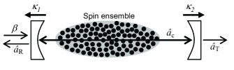
Figure 1: The physical setup under consideration. A spin ensemble is coupled to a cavity field $\hat{a}_{\mathrm{c}}$, which is subjected to decay through the two mirrors with field-decay rates $\kappa_{1}$ and $\kappa_{2}$. For diagnostics purposes an external driving field $\beta$ may be applied giving rise to reflected and transmitted fields, $\hat{a}_{\mathrm{R}}$ and $\hat{a}_{\mathrm{T}}$, as discussed in Sec. V.

III Dynamical evolution of an inverted medium inside a cavity: Mean values

The present section considers the evolution of mean values of the cavity field and the spin components for an inverted spin state. The calculations assume a resonant coupling between the cavity and the spins, $\Delta_{\mathrm{cs}}=0$, in which case the effects under study are strongest.

III.1 A stability criterion using the effective cooperativity parameter

Consider the following mean value equations, which have been derived under the Holstein-Primakoff approximation ($\hat{\sigma}_{z}^{(j)}\approx 1$) in absence of external driving:

$$\frac{\partial\langle\hat{a}_{\mathrm{c}}\rangle}{\partial t} =-(\kappa+i\Delta_{\mathrm{cs}})\langle\hat{a}_{\mathrm{c}}\rangle-i\sum_{j=1}^{N}g_{j}\langle\hat{\sigma}_{-}^{(j)}\rangle,$$ (2)

$$\frac{\partial\langle\hat{\sigma}_{-}^{(j)}\rangle}{\partial t} =-(\gamma_{\perp}+i\Delta_{j})\langle\hat{\sigma}_{-}^{(j)}\rangle+ig_{j}\langle\hat{a}_{\mathrm{c}}\rangle.$$ (3)

We note that if $\langle\hat{a}_{\mathrm{c}}\rangle$ is real and positive, the second term of Eq. (3) will drive $\langle\hat{\sigma}_{-}^{(j)}\rangle$ toward positive imaginary values. In turn, the second term of Eq. (2) will drive $\langle\hat{a}_{\mathrm{c}}\rangle$ further along the positive real axis, and the physical system is thus unstable due to the gain provided by the inverted sample. This scenario resembles to a large extent a laser, and normal laser operation is initiated when the gain medium is able to balance the optical losses of the cavity; however, the case under study here differs from normal laser operation by the fact that the inverted spin medium behaves coherently. Accordingly, a large cavity loss (i.e. a large $\kappa$) is not the only way to counter-act the inherent instability, but dephasing due to inhomogeneous broadening will also contribute.

In analogy to threshold conditions for normal laser operation, a stability criterion can be derived for our spin-cavity system by searching for a critical cavity-coupling parameter, $\kappa_{\mathrm{c}}$, which allows for a non-zero steady-state solution for $\langle\hat{a}_{\mathrm{c}}\rangle$ and $\langle\hat{\sigma}_{j}^{(j)}\rangle$. Then increasing (decreasing) solutions versus time are expected when $\kappa<\kappa_{\mathrm{c}}$ ($\kappa>\kappa_{\mathrm{c}}$). To this end, consider first Eq. (3) in steady state: $\langle\hat{\sigma}_{-}^{(j)}\rangle=\frac{ig_{j}\langle\hat{a}_{\mathrm{c}}\rangle}{\gamma_{\perp}+i\Delta_{j}}$, which inserted into Eq. (2) in steady state leads to: $(\kappa+i\Delta_{\mathrm{cs}})\langle\hat{a}_{\mathrm{c}}\rangle=\sum_{j}\frac{g_{j}^{2}}{\gamma_{\perp}+i\Delta_{j}}\langle\hat{a}_{\mathrm{c}}\rangle$. We shall restrict ourselves to inhomogeneous broadening with $\Delta_{j}$ distributed symmetrically around zero, in which case $\Delta_{\mathrm{cs}}=0$ is indeed the relevant choice. The above equation can be satisfied for a non-zero $\langle\hat{a}_{\mathrm{c}}\rangle$ provided that $\kappa$ attains the critical value:

$$\kappa_{\mathrm{c}}=g_{\mathrm{ens}}^{2}\int_{-\infty}^{\infty}\frac{f(\Delta)d\Delta}{\gamma_{\perp}+i\Delta}\equiv\frac{g_{\mathrm{ens}}^{2}}{\Gamma},$$ (4)

where we assumed the distributions of $g_{j}$ and $\Delta_{j}$ to be uncorrelated. Furthermore, the continuum limit was taken by using the spin-resonance-frequency distribution $f(\Delta)$ normalized such that $\int_{-\infty}^{\infty}f(\Delta)d\Delta=1$. The characteristic width $\Gamma$ of the inhomogeneous distribution was implicitly defined, and the requirement of $\kappa>\kappa_{\mathrm{c}}$ for stability can be reformulated in terms of the effective cooperativity parameter, $C$:

$$C=\frac{g_{\mathrm{ens}}^{2}}{\kappa\Gamma}<1.$$ (5)

III.2 Homogeneous broadening

Even though the main focus of this paper is inhomogeneous broadening, it is convenient to know the effects of homogeneous broadening for comparison. From Eq. (4) it follows immediately that $\Gamma=\gamma_{\perp}$ in this case ($f(\Delta)$ is a $\delta$-function). In fact, Eqs. (2) and (3) can be reformulated in terms of the effective spin component $\hat{S}_{-}^{\mathrm{eff}}=\sum_{j=1}^{N}\frac{g_{j}}{\mathrm{bar}{g}}\hat{\sigma}_{-}^{(j)}$, where $\mathrm{bar}{g}^{2}=\sum_{j=1}^{N}g_{j}^{2}/N$, and the inverted spin-state problem is only two-dimensional:

$$\frac{\partial}{\partial t}\begin{bmatrix}\langle\hat{a}_{\mathrm{c}}\rangle\\ \langle\hat{S}_{-}^{\mathrm{eff}}\rangle\end{bmatrix}=\begin{bmatrix}-(\kappa+i\Delta_{\mathrm{cs}})&-i\mathrm{bar}{g}\\ i\mathrm{bar}{g}N&-\gamma_{\perp}\end{bmatrix}\begin{bmatrix}\langle\hat{a}_{\mathrm{c}}\rangle\\ \langle\hat{S}_{-}^{\mathrm{eff}}\rangle\end{bmatrix}.$$ (6)

On resonance, $\Delta_{\mathrm{cs}}=0$, the eigenvalues of this linear set of equations are:

$$\lambda_{\pm}=-\frac{\kappa+\Gamma}{2}\left(1\mp\sqrt{1+\frac{4(C-1)\kappa\Gamma}{(\kappa+\Gamma)^{2}}}\right).$$ (7)

Clearly, when $C<1$ both eigenvalues are negative and the inverted spin state with $\langle\hat{a}_{\mathrm{c}}\rangle=\langle\hat{S}_{-}^{\mathrm{eff}}\rangle=0$ is a stable solution.

III.3 Inhomogeneous broadening

In order to examine the dynamical evolution of the spin-cavity system with analytical methods in the case of inhomogeneous broadening, it is convenient to treat Eqs. (2) and (3) in Fourier space. In order to handle also exponentially increasing solutions, we re-write the dynamical variables as $\langle\hat{a}_{\mathrm{c}}\rangle=\langle\tilde{a}_{\mathrm{c}}\rangle e^{\eta t}$ and $\langle\hat{\sigma}_{-}^{(j)}\rangle=\langle\tilde{\sigma}_{-}^{(j)}\rangle e^{\eta t}$. Assume also that $\langle\hat{a}_{\mathrm{c}}\rangle=\langle\hat{\sigma}_{-}^{(j)}\rangle=0$ when $t<0$, which indeed presents a mathematical solution to the differential equations. Then, at $t=0$ we change abruptly the cavity-field mean value $\langle\hat{a}_{\mathrm{c}}\rangle\rightarrow\alpha$ and study the subsequent dynamics. This scenario is governed by a modified version of Eqs. (2) and (3) taken at resonance, $\Delta_{\mathrm{cs}}=0$:

$$\frac{\partial\langle\tilde{a}_{\mathrm{c}}\rangle}{\partial t} =\alpha\delta(t)-(\kappa+\eta)\langle\tilde{a}_{\mathrm{c}}\rangle-i\sum_{j=1}^{N}g_{j}\langle\tilde{\sigma}_{-}^{(j)}\rangle,$$ (8)

$$\frac{\partial\langle\tilde{\sigma}_{-}^{(j)}\rangle}{\partial t} =-(\gamma_{\perp}+\eta+i\Delta_{j})\langle\tilde{\sigma}_{-}^{(j)}\rangle+ig_{j}\langle\tilde{a}_{\mathrm{c}}\rangle.$$ (9)

The latter of these can be integrated formally: $\langle\tilde{\sigma}_{-}^{(j)}(t)\rangle=ig_{j}\int_{0}^{t}e^{-(\gamma_{\perp}+\eta+i\Delta_{j})(t-t^{\prime})}\langle\tilde{a}_{\mathrm{c}}(t^{\prime})\rangle dt^{\prime}$, which in turn can be inserted into Eq. (8):

$$\frac{\partial\langle\tilde{a}_{\mathrm{c}}\rangle}{\partial t}=\alpha\delta(t)-(\kappa+\eta)\langle\tilde{a}_{\mathrm{c}}\rangle+\int_{0}^{t}\tilde{K}(t-t^{\prime})\langle\tilde{a}_{\mathrm{c}}(t^{\prime})\rangle,$$ (10)

where $\tilde{K}(t)=\sum_{j=1}^{N}g_{j}^{2}e^{-(\gamma_{\perp}+\eta+i\Delta_{j})t}$. Now, by defining the positive-time version of $\tilde{K}$ by $\tilde{K}^{+}(t)=\tilde{K}(t)\cdot\theta(t)$, where $\theta(t)$ is the Heaviside step function, and by remembering that $\langle\tilde{a}_{\mathrm{c}}(t^{\prime})\rangle=0$ when $t^{\prime}<0$, the above integration can be extended to plus/minus infinity. Using the Fourier transform, $\langle\tilde{a}_{\mathrm{c}}(\omega)\rangle=\int_{-\infty}^{\infty}\langle\tilde{a}_{\mathrm{c}}(t)\rangle e^{i\omega t}dt$ and $\langle\tilde{a}_{\mathrm{c}}(t)\rangle=\frac{1}{2\pi}\int_{-\infty}^{\infty}\langle\tilde{a}_{\mathrm{c}}(\omega)\rangle e^{-i\omega t}d\omega$, we find:

$$\langle\tilde{a}_{\mathrm{c}}(\omega)\rangle=\frac{\alpha}{\kappa+\eta-i\omega-\tilde{K}^{+}(\omega)}.$$ (11)

The Fourier transform $\tilde{K}^{+}(\omega)$ can be expressed in the continuum limit as:

$$\tilde{K}^{+}(\omega)=-ig_{\mathrm{ens}}^{2}\int_{-\infty}^{\infty}\frac{f(\Delta)d\Delta}{\Delta-\omega-i(\gamma_{\perp}+\eta)}.$$ (12)

III.3.1 Lorentzian broadening

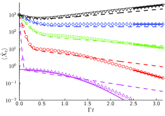
Figure 2: (Color online) Cavity-field decay versus time when the inhomogeneous broadening is Lorentzian [dashed lines, from Eq. (15)] and Gaussian [symbols, numerical simulation]. In all cases, $g_{\mathrm{ens}}=2\Gamma$ and $\gamma_{\perp}=0$, while $\kappa$ is varied such that $C$ attains the values of 0.05 (magenta tip-up triangles), 0.2 (red circles), 0.5 (green squares), 1 (blue diamonds), and 2 (black tip-down triangles). The vertical axis contains $\langle\hat{X}_{\mathrm{c}}\rangle=(\langle\hat{a}_{\mathrm{c}}\rangle+\langle\hat{a}^{\dagger}_{\mathrm{c}}\rangle)/\sqrt{2}$. In the range $\Gamma t\geq 2.5$ the slope of the Gaussian-broadening decay curves are compared to a numerically determined value (solid lines) as discussed in the text prior to Eq. (17). The solid curve through the magenta tip-up triangles is given by Eq. (18).

For a Lorentzian broadened spin ensemble with $f(\Delta)=\frac{w/2\pi}{\Delta^{2}+w^{2}/4}$, where $w$ is the FWHM (full width at half maximum), the characteristic width of Eq. (4) becomes: $\Gamma=\frac{w}{2}+\gamma_{\perp}$. Furthermore, Eq. (12) can be written (using the residue theorem):

$$\tilde{K}^{+}(\omega)=\frac{g_{\mathrm{ens}}^{2}}{\Gamma+\eta-i\omega},$$ (13)

and inserting this result into Eq. (11) leads to:

$$\langle\tilde{a}_{\mathrm{c}}(\omega)\rangle=\frac{\alpha(i\omega-\Gamma-\eta)}{(\omega-i[\lambda_{+}-\eta])(\omega-i[\lambda_{-}-\eta])},$$ (14)

where $\lambda_{\pm}$ are the solutions given in Eq. (7). The inverse Fourier transform is now invoked, leading to ($t>0$):

$$\langle\hat{a}_{\mathrm{c}}(t)\rangle=\alpha\frac{(\lambda_{+}+\Gamma)e^{\lambda_{+}t}-(\lambda_{-}+\Gamma)e^{\lambda_{-}t}}{\lambda_{+}-\lambda_{-}},$$ (15)

and $\langle\hat{a}_{\mathrm{c}}(t)\rangle=0$ when $t<0$. This expression is independent of $\eta$ as it should be; however, for the Fourier transform $\langle\tilde{a}_{\mathrm{c}}(\omega)\rangle$ to exist, the condition $\eta>\lambda_{+}$ must be fulfilled, which in fact also ensures that both poles in Eq. (14) reside in the lower complex half-plane.

III.3.2 Gaussian broadening

For a Gaussian broadened spin ensemble with $f(\Delta)=\frac{1}{\sqrt{2\pi}\sigma_{\Delta}}e^{-\Delta^{2}/2\sigma_{\Delta}^{2}}$, where $\sigma_{\Delta}$ is the standard deviation of the distribution (connected to the FWHM by $w=\sigma_{\Delta}\sqrt{8\ln(2)}$) the characteristic width (4) is given by: $\Gamma=\sqrt{\frac{2}{\pi}}\frac{\sigma_{\Delta}}{w(z)}$, where the complex error function is given by $w(z)=e^{-z^{2}}\mathrm{erfc}(-iz)$ with $\mathrm{erfc}(\cdot)$ being the complementary error function Abramowitz and Stegun (1972) and $z=\frac{i\gamma_{\perp}}{\sqrt{2}\sigma_{\Delta}}$. Equation (12) reads in this case:

$$\tilde{K}^{+}(\omega)=\sqrt{\frac{\pi}{2}}\frac{g_{\mathrm{ens}}^{2}}{\sigma_{\Delta}}w(\tilde{z}),$$ (16)

where $\tilde{z}=\frac{\omega+i(\gamma_{\perp}+\eta)}{\sqrt{2}\sigma_{\Delta}}$. It is not possible to write a general analytic expression for the inverse transform $\langle\hat{a}_{\mathrm{c}}(t)\rangle$; however, we shall calculate $\langle\hat{a}_{\mathrm{c}}(t)\rangle$ by numerical integration of Eq. (34) with a real, non-zero $X_{\mathrm{c}}=\sqrt{2}\alpha$ as initial condition at $t=0$, and limiting cases will be compared to analytical estimates. Such numerical simulations are shown (with symbols) in Fig. 2 for various values of the effective cooperativity parameter $C$, and comparison to the Lorentzian-broadened case is made (by dashed lines, maintaining $\kappa$ and $\Gamma$). The following points can be noted: (I) the initial decay seems similar for Lorentzian and Gaussian broadening, (II) in the long-time limit for Gaussian broadening the decay seems to be exponential, and (III) when the coupling is weak ($C\ll 1$) the curves for Gaussian broadening appear to have a significant quadratic content when plotted on the logarithmic vertical scale.

The single-exponential parts of the decay curves (with rate $\lambda$) correspond to the poles of Eq. (11), i.e. solutions ($\omega=i\lambda$) to the equation $\kappa-i\omega=\sqrt{\frac{\pi}{2}}\frac{g_{\mathrm{ens}}^{2}}{\sigma_{\Delta}}w(\tilde{z})$ taking $\eta=0$. Provided that $|\lambda|\gg\sigma_{\Delta}$ for the initial fast decay, we take advantage of the series expansion, $w(z)\approx\frac{i}{\sqrt{\pi}z}$ when $|z|\gg 1$, and reach the condition: $(\lambda+\kappa)(\lambda+\gamma_{\perp})=g_{\mathrm{ens}}^{2}$. This is exactly the eigen-value equation for the homogeneous system of equations (6), and the solution $\lambda$ is equal to $\lambda_{-}$ in Eq. (7) with $\Gamma=\gamma_{\perp}$. From a physical perspective, the narrow feature of the Gaussian broadening cannot be resolved on the initial fast time scales. The long-time limit of the decay for Gaussian broadening is compared in Fig. 2 by solid lines to the rate $\lambda$ found by locating numerically another pole of Eq. (11). In the vicinity of the stability threshold, $\kappa\approx\kappa_{\mathrm{c}}$ such that $|\lambda|\ll\sigma_{\Delta}$, the value of $\lambda$ can be approximated by using the series expansion, $w(z)\approx 1+\frac{2iz}{\sqrt{\pi}}-z^{2}$ when $|z|\ll 1$, leading to:

$$\lambda\approx\frac{\kappa_{\mathrm{c}}-\kappa}{1+\frac{g_{\mathrm{ens}}^{2}}{\sigma_{\Delta}^{2}}}+\sqrt{\frac{\pi}{8}}\frac{g_{\mathrm{ens}}^{2}}{\sigma_{\Delta}^{3}}\frac{(\kappa_{\mathrm{c}}-\kappa)^{2}}{\left(1+\frac{g_{\mathrm{ens}}^{2}}{\sigma_{\Delta}^{2}}\right)^{3}}.$$ (17)

Finally, the weak-coupling limit, $C\ll 1$, can be calculated directly from Eqs. (8) and (9), provided that $\kappa$ is faster than the remaining dynamical processes. In a first approximation, $\langle\hat{a}_{\mathrm{c}}(t)\rangle=\alpha e^{-\kappa t}$, since the spins will contribute little due to the low coupling. Secondly, during the initial decay of the cavity field, each spin component acquires a small value: $\langle\hat{\sigma}_{-}^{(j)}\rangle=\frac{ig_{j}\alpha}{\kappa}$, which is derived by integrating the second term of Eq. (9); the first term can be neglected on this fast time scale. Thirdly, after the initial cavity decay, the spins evolve freely due to the low coupling: $\frac{\partial}{\partial t}\langle\hat{\sigma}_{-}^{(j)}\rangle=-(\gamma_{\perp}+i\Delta_{j})\langle\hat{\sigma}_{-}^{(j)}\rangle$, and the cavity field follows the spins adiabatically in this regime:

$$\langle\hat{a}_{\mathrm{c}}(t)\rangle\approx-\frac{i}{\kappa}\sum_{j=1}^{N}g_{j}\langle\hat{\sigma}_{-}^{(j)}\rangle=\frac{\alpha g_{\mathrm{ens}}^{2}}{\kappa^{2}}e^{-\frac{1}{2}\sigma_{\Delta}^{2}t^{2}-\gamma_{\perp}t},$$ (18)

where the continuum limit of the inhomogeneous frequency distribution was taken in the last step. Alternatively, when $C\ll 1$, Eq. (11) can be approximated: $\langle\tilde{a}_{\mathrm{c}}(\omega)\rangle\approx\frac{\alpha}{\kappa-i\omega}+\frac{\alpha g_{\mathrm{ens}}^{2}}{(\kappa-i\omega)^{2}}\sqrt{\frac{\pi}{2}}\frac{w(z)}{\sigma_{\Delta}}\approx\frac{\alpha}{\kappa-i\omega}+\frac{\alpha g_{\mathrm{ens}}^{2}}{\kappa^{2}}\sqrt{\frac{\pi}{2}}\frac{w(z)}{\sigma_{\Delta}}$, where the second step considers only the low-frequency parts of the second term ($w(z)$ varies on the frequency scale of $\sigma_{\Delta}\ll\kappa$). The inverse Fourier transform of this approximated $\langle\tilde{a}_{\mathrm{c}}(\omega)\rangle$ is $\alpha e^{-\kappa t}$ plus the term found in Eq. (18). The lower curve (magenta tip-up triangles, $C=0.05$) in Fig. 2 follows Eq. (18) to a large extent.

IV Dynamical evolution of an inverted medium inside a cavity: Quadratic moments

The calculation of the dynamical evolution of mean values in the preceding section presents one of the main results of the present manuscript. However, we wish to back up these mean-field results by a calculation of second moments — a mean-value stabilized spin-cavity system would be of less relevance if e.g. the variance of the spin components and the cavity field increased without limits. Such an unlimited increase will also render the spin-cavity system inapplicable for quantum-memory purposes.

The case of homogeneous broadening is treated analytically while inhomogeneous broadening requires numerical treatment. In any case, the calculations follow the general procedure outlined in appendix  A.

IV.1 Homogeneous broadening

Assume that $\Delta_{j}=0$ and $g_{j}=g$ for all spins. For an inverted spin sample on resonance with mean values $X_{\mathrm{c}}=P_{\mathrm{c}}=S_{x}=S_{y}=0$, $S_{z}=N$, and $\Delta_{\mathrm{cs}}=0$, we introduce the vector of second moments, $\mathbf{x}=[\langle\delta\hat{X}_{\mathrm{c}}^{2}\rangle$ $\langle\delta\hat{P}_{\mathrm{c}}^{2}\rangle$ $\langle\delta\hat{S}_{x}^{2}\rangle$ $\langle\delta\hat{S}_{y}^{2}\rangle$ $\langle\delta\hat{S}_{x}\delta\hat{P}_{\mathrm{c}}\rangle$ $\langle\delta\hat{S}_{y}\delta\hat{X}_{\mathrm{c}}\rangle]^{\mathrm{T}}$. Following Eq. (36) in the appendix, they obey the following set of coupled equations, $\frac{\partial\mathbf{x}}{\partial t}=\mathbf{Q}\mathbf{x}+\mathbf{r}$, where

$$\mathbf{Q}=\begin{bmatrix}-2\kappa&0&0&0&0&-\sqrt{2}g\\ 0&-2\kappa&0&0&-\sqrt{2}g&0\\ 0&0&-2\gamma_{\perp}&0&-2\sqrt{2}gN&0\\ 0&0&0&-2\gamma_{\perp}&0&-2\sqrt{2}gN\\ 0&-\sqrt{2}gN&-\frac{g}{\sqrt{2}}&0&-(\kappa+\gamma_{\perp})&0\\ -\sqrt{2}gN&0&0&-\frac{g}{\sqrt{2}}&0&-(\kappa+\gamma_{\perp})\end{bmatrix},\quad\mathbf{r}=\begin{bmatrix}\kappa\\ \kappa\\ 2\gamma_{\perp}N\\ 2\gamma_{\perp}N\\ 0\\ 0\end{bmatrix}.$$ (19)

In fact, an inhomogeneous distribution of the coupling constants, $g_{j}$, can be incorporated in the above equations by merely replacing $\hat{S}_{x}\rightarrow\hat{S}_{x}^{\mathrm{eff}}$, $\hat{S}_{y}\rightarrow\hat{S}_{y}^{\mathrm{eff}}$, and $g\rightarrow\mathrm{bar}{g}$. The matrix $\mathbf{Q}$ has three doubly-degenerate eigenvalues. Two of these are given by $\lambda=2\lambda_{\pm}$, i.e. by twice the values found in Eq. (7), and the third one is $\lambda=-(\kappa+\gamma_{\perp})$. Hence, the same condition $C<1$, ensures that both the first and second moments are stable and converge to their steady-state values. Solving $\frac{\partial\mathbf{x}}{\partial t}=\mathbf{Q}\mathbf{x}+\mathbf{r}=0$, these read:

$$\begin{split}\langle\delta\hat{X}_{\mathrm{c}}^{2}\rangle&=\langle\delta\hat{P}_{\mathrm{c}}^{2}\rangle=\frac{1}{2}\cdot\frac{1-C\frac{\kappa-\Gamma}{\kappa+\Gamma}}{1-C},\\ \langle\delta\hat{S}_{x}^{\mathrm{eff}\,2}\rangle&=\langle\delta\hat{S}_{y}^{\mathrm{eff}\,2}\rangle=N\cdot\frac{1+C\frac{\kappa-\Gamma}{\kappa+\Gamma}}{1-C},\\ \langle\delta\hat{S}_{x}^{\mathrm{eff}}\delta\hat{P}_{\mathrm{c}}\rangle&=\langle\delta\hat{S}_{y}^{\mathrm{eff}}\delta\hat{X}_{\mathrm{c}}\rangle=-\sqrt{\frac{N}{2}}\frac{2g_{\mathrm{ens}}}{(\kappa+\Gamma)(1-C)},\end{split}$$ (20)

where $\Gamma=\gamma_{\perp}$ for homogeneous broadening. We note that the levels of $\frac{1}{2}$ and $N$ correspond to the variance of the minimum-uncertainty states for the cavity field and the collective spin, respectively. When approaching the stability point $C\rightarrow 1$ from below, the variances diverge.

IV.2 Inhomogeneous broadening

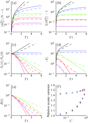
Figure 3: (Color online) Panels (a-e) show various dynamical parameters versus time with fixed $g_{\mathrm{ens}}=2\Gamma$ and varying $\kappa$, such that $C$ attains the values $0.05$ (magenta), $0.2$ (red), $0.5$ (green), $1$ (blue), and $2$ (black), represented in the order from the the lower to the upper sets of dashed and solid curves in all plots. Solid lines have been calculated for Gaussian inhomogeneous broadening ($\gamma_{\perp}=0$), while the dashed lines correspond to both Lorentzian broadening ($\gamma_{\perp}=0$) and homogeneous broadening ($\gamma_{\perp}=\Gamma$). (a) Excess variance of $\hat{S}_{x}$ relative to the coherent-state value of $N$. (b) Excess variance of $\hat{P}_{\mathrm{c}}$ relative to the coherent-state value of $\frac{1}{2}$. (c) The mean value of $S_{x}$ normalized to $S_{x}(t=0)$. (d) The mean value of $\hat{P}_{\mathrm{c}}$ in arbitrary units. (e) The relative deviation of $\langle\delta\hat{S}_{x}^{2}\rangle$ from its steady-state value, $R(t)$, see the text for details. (f) The Gaussian-broadened steady-state excess variance $[\langle\delta\hat{S}_{x}^{2}(\infty)\rangle/N-1]$ (circles) or $[2\langle\delta\hat{P}_{\mathrm{c}}^{2}(\infty)\rangle-1]$ (diamonds), relative to the corresponding values from Eq. (20). The results are very similar for the different coupling strengths $g_{\mathrm{ens}}=3\Gamma$ (red), $g_{\mathrm{ens}}=4\Gamma$ (green), and $g_{\mathrm{ens}}=5\Gamma$ (blue).

For the case of inhomogeneous broadening we use numerical simulation of Eqs. (34) and (36) for calculating the dynamical evolution. We use only a single value for $g_{m}$ but choose either a Lorentzian or Gaussian shaped distribution of $\Delta_{m}$. As a starting point, all spins are prepared in the inverted coherent state being slightly displaced: $S_{z}^{(m)}=N_{m}$, $S_{y}^{(m)}=0$, and $S_{x}^{(m)}=\theta S_{z}^{(m)}$ where $\theta=10^{-3}$, and the cavity is prepared in the vacuum state. Leaving the spin-cavity system to evolve from this initial state, we study as function of time a representative set of mean values and variances: $S_{x}=\sum_{m=1}^{M}S_{x}^{(m)}$, $P_{\mathrm{c}}$, $\langle\delta\hat{S}_{x}^{2}\rangle=\sum_{m,n=1}^{M}\langle\delta\hat{S}_{x}^{(m)}\delta\hat{S}_{x}^{(n)}\rangle$, and $\langle\delta\hat{P}_{\mathrm{c}}^{2}\rangle$, the results have been plotted in Fig. 3.

Panels (a) and (b) of this figure show how the variances, $\langle\delta\hat{S}_{x}^{2}\rangle$ and $\langle\delta\hat{P}_{\mathrm{c}}^{2}\rangle$, increase from their initial values of $N$ and $\frac{1}{2}$, respectively. As can be seen, in the stable region with $C<1$ these variances converge to a steady-state value while for $C\geq 1$ the curves increase without limits. The solid lines correspond to a Gaussian distribution while the dashed lines correspond to a homogeneously broadened sample with $\Gamma=\gamma_{\perp}$, which coincides with the simulations for a Lorentzian broadened sample with $\gamma_{\perp}=0$ and $\Gamma=\frac{w}{2}$. At the same time, the mean values of $\hat{S}_{x}$ and $\hat{P}_{\mathrm{c}}$ have been plotted in panel (c) and (d), which confirm that solutions increase or decrease versus time when $C>1$ or $C<1$, respectively. We note that the features and interpretation of these graphs are very similar to those of Fig. 2; only the initial state is different in the two figures. In order to show the time scale of the dynamical evolution of variances, the deviation of $\langle\delta\hat{S}_{x}^{2}(t)\rangle$ from its asymptotic value of $\langle\delta\hat{S}_{x}^{2}(\infty)\rangle$ has been shown in panel (e) relative to the entire dynamical range, i.e. the vertical scale is the ratio: $R(t)=\frac{\langle\delta\hat{S}_{x}^{2}(\infty)\rangle-\langle\delta\hat{S}_{x}^{2}(t)\rangle}{\langle\delta\hat{S}_{x}^{2}(\infty)\rangle-\langle\delta\hat{S}_{x}^{2}(0)\rangle}$. Noting that in panel (e) the horizontal axis spans only half the time as compared to panel (c), it can be seen that the variance $\langle\delta\hat{S}_{x}^{2}\rangle$ approaches its asymptotic value approximately twice as fast as the decay of the mean value $S_{x}$ toward zero. This is no surprise for the homogeneous or Lorentzian case since we already observed that the three characteristic eigenvalues of the problem, $2\lambda_{+}$, $2\lambda_{-}$, and $\lambda_{+}+\lambda_{-}$, relate closely to the eigen values of the mean value equation (7). The similarity of the solid lines in panels (c) and (e) demonstrate that this holds qualitatively also for the case of Gaussian broadening. Finally, it can be observed from panels (a) and (b) that in the case of Gaussian broadening (solid lines), the variances $\langle\delta\hat{S}_{x}^{2}\rangle$ and $\langle\delta\hat{P}_{\mathrm{c}}^{2}\rangle$ converge to values which are slightly higher than those give by Eq. (20) when simply inserting the corresponding values for $\kappa$, $\Gamma$, and $C$ (dashed lines). The ratio of solid-to-dashed lines in panels (a) and (b) have been shown in panel (f) with circles and diamonds, respectively, and varying values for the ratio $g_{\mathrm{ens}}/\Gamma$ have been examined. We conclude that Eq. (20) is not accurate for a Gaussian inhomogeneous distribution although the qualitative features remain.

V External probing of the spin sample

The linear response of the spin ensemble can be probed by applying a weak, external field $\beta$ and measuring the reflected or transmitted field as depicted in Fig. 1. Such a measurement enables the determination of $C$ from a non-inverted sample and also allows for assessing the efficiency of the spin-inversion process. Assuming the cavity to be resonant with the spins, $\Delta_{\mathrm{cs}}=0$, the following mean-value equations are valid under the Holstein-Primakoff approximation:

$$\frac{\partial\langle\hat{a}_{\mathrm{c}}\rangle}{\partial t} =-\kappa\langle\hat{a}_{\mathrm{c}}\rangle-i\sum_{j=1}^{N}g_{j}\langle\hat{\sigma}_{-}^{(j)}\rangle+\sqrt{2\kappa_{1}}\beta$$ (21)

$$\frac{\partial\langle\hat{\sigma}_{-}^{(j)}\rangle}{\partial t} =-(\gamma_{\perp}+i\Delta_{j})\langle\hat{\sigma}_{-}^{(j)}\rangle+ipg_{j}\langle\hat{a}_{\mathrm{c}}\rangle,$$ (22)

where $p=1$ for an inverted sample and $p=-1$ for a non-inverted sample. By applying a monochromatic external field, $\beta(t)=\beta_{0}e^{-i\Delta_{\mathrm{e}}t}$, the cavity-field mean value can be shown to be:

$$\langle\hat{a}_{\mathrm{c}}(t)\rangle=\frac{\sqrt{2\kappa_{1}}\beta(t)}{\kappa-i\Delta_{\mathrm{e}}-pg_{\mathrm{ens}}^{2}\int_{-\infty}^{\infty}\frac{f(\Delta)d\Delta}{\gamma_{\perp}+i(\Delta-\Delta_{\mathrm{e}})}}.$$ (23)

In fact, this is a particular solution to the differential equation and we assume that the homogeneous solution has relaxed to zero; this relaxation process was the topic of Sec. III, and for an inverted sample ($p=1$) the calculations only make sense if the stability criterion is met, $C<1$. The integral in the denominator of the above equation is equal to $[\Gamma-i\Delta_{\mathrm{e}}]^{-1}$ for Lorentzian broadening and equal to $\sqrt{\frac{\pi}{2}}\frac{w(z_{\mathrm{e}})}{\sigma_{\Delta}}$ with $z_{\mathrm{e}}=\frac{\Delta_{\mathrm{e}}+i\gamma_{\perp}}{\sqrt{2}\sigma_{\Delta}}$ for Gaussian broadening. When the driving is resonant, $\Delta_{\mathrm{e}}=0$, the integral is equal to $\Gamma^{-1}$ for any (symmetric) distribution according to Eq. (4).

Now, the reflected and transmitted fields relate to the cavity field by Collett and Gardiner (1984): $\langle\hat{a}_{\mathrm{R}}\rangle=\sqrt{2\kappa_{1}}\langle\hat{a}_{\mathrm{c}}\rangle-\beta$ and $\langle\hat{a}_{\mathrm{T}}\rangle=\sqrt{2\kappa_{2}}\langle\hat{a}_{\mathrm{c}}\rangle$. This enables a calculation of the complex reflection and transmission coefficients, $r=\frac{\langle\hat{a}_{\mathrm{R}}\rangle}{\beta}$ and $t=\frac{\langle\hat{a}_{\mathrm{T}}\rangle}{\beta}$, respectively. Selected examples have been plotted in Fig. 4 for a Lorentzian inhomogeneous broadening (a Gaussian profile presents qualitatively similar results). When $C$ increases beyond unity, the bare-cavity transmission spectrum is significantly modified by the presence of the spin ensemble and the well-known normal-mode splitting occurs Zhu et al. (1990). Note that $C=1$ corresponds to the case where the transmission coefficient is reduced from unity to one half (for a symmetric cavity). We also note that the transmission spectrum exists for an inverted sample when $C<1$ (the dotted curve exemplifies this) and that the transmission coefficient may exceed unity due to the inherent gain of the inverted sample.

A particular relation, which is useful for a simple estimation of the effective cooperativity parameter, is given by the connection of $C$ to the values of $r$ and $t$ for any (symmetric) distribution on resonance ($\Delta_{\mathrm{e}}=0$):

$$pC=\frac{r-\frac{\kappa_{1}-\kappa_{2}}{\kappa_{1}+\kappa_{2}}}{r+1}=1-\frac{2\sqrt{\kappa_{1}\kappa_{2}}}{\kappa}\cdot\frac{1}{t}.$$ (24)

The fact that the reflection and transmission coefficients may exceed unity clearly demonstrates that the excitation level of the spin ensemble must account for the energy balance. This fact is disguised by the Holstein-Primakoff approximation, but it is possible to estimate the effect in a mean-field theory on resonance ($\Delta_{\mathrm{cs}}=0$, see the appendix for details):

$$\frac{\partial S_{z}}{\partial t}=-\frac{4pg_{\mathrm{ens}}^{2}|a_{\mathrm{c}}|^{2}}{\Gamma}.$$ (25)

We stress that this holds also for a non-inverted sample ($p=-1$), in which case energy quanta leak from the cavity into the continuous spin ensemble with a rate proportional to a squared matrix element, $\sim\frac{g_{\mathrm{ens}}^{2}}{N}$, times the density of states, $\sim\frac{N}{\Gamma}$, resembling the usual Fermi’s-Golden-Rule expression for decay of a quantum system due to the coupling to a broad-bandwidth reservoir. In order that this de-polarizing effect is kept small, the duration $T$ of the external driving must be short enough so that $\left|\frac{\partial S_{z}}{\partial t}\right|T\ll N$. This is equivalent to: $n_{\mathrm{ph}}\ll\frac{\kappa}{\kappa_{1}}\cdot\frac{(1-pC)^{2}}{8|pC|}\cdot N$, where $n_{\mathrm{ph}}=|\beta|^{2}T$ is the total number of photons supplied by the external driving field during the experiment. Clearly, for an inverted sample approaching the point of instability, $pC\rightarrow 1$, the allowed number of photons decreases significantly below $N$.

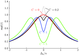
Figure 4: (Color online) The real part of the transmission coefficient versus external driving frequency. The calculations assume a Lorentzian profile, $\kappa_{1}=\kappa_{2}$, $\kappa=10\Gamma$, and $g_{\mathrm{ens}}$ is varied in order to obtain the $C$-values marked on the curves. Solid lines are non-inverted ($p=-1$) while the dotted line for $C=0.2$ corresponds to an inverted sample ($p=1$).

VI Discussion

The stability criterion of Eq. (5) and the dynamical evolution of the spin-cavity system below and above the point of stability present the main result of this manuscript. The results of Sec. IV, in particular panels (a-d) of Fig. 3, demonstrate that the stability criterion refers to both the mean values and the second moments. This follows naturally from the fact that the same matrices govern the linear sets of equations for the first and second moments, as shown in the appendix.

Understanding the free evolution of an inverted spin ensemble in a cavity is of high importance for spin-refocusing techniques. Such refocusing could improve spin-based quantum memory protocols in cavities. However, the storage and retrieval part of such a protocol Kubo et al. (2011) would typically be implemented in the strong-coupling regime, $g_{\mathrm{ens}}\gg\kappa,\Gamma$, i.e. with $C\gg 1$, and the ability to tune the value of $C$ during the experimental protocol would then be necessary. We also note that the spins can effectively be decoupled from the cavity field by a large detuning $\Delta_{\mathrm{cs}}$. The discussion after Eq. (18) can be stated more generally as $\langle\hat{a}_{\mathrm{c}}(\omega)\rangle\approx\frac{\alpha}{\kappa+i(\Delta_{\mathrm{cs}}-\omega)}+\frac{\alpha K^{+}(\omega)}{[\kappa+i\Delta_{\mathrm{cs}}]^{2}}$ when $|\kappa+i\Delta_{\mathrm{cs}}|$ is large compared to the frequency width of $K^{+}(\omega)$. This equation reflects the fact that the cavity field follows adiabatically the evolution of the (effectively) uncoupled spin ensemble (the second term depends on $\omega$ through $K^{+}(\omega)$ only), which in turn is largely given by the Fourier components of $f(\Delta)$ through the relation (12). Note that a broad and smooth distribution $f(\Delta)$ is required in general, coupled or uncoupled, if a fast relaxation of both the cavity field and the spin components is desired.

The diagnostics tools presented in Sec. V have been derived for a perfectly polarized spin ensemble ($p=\pm 1$). However, as exemplified in the appendix by using a suitable sub-ensemble distribution, we may argue that the results of Sec. V hold for a non-perfect polarization also, $-1\leq p\leq 1$. The Holstein-Primakoff approximation corresponds to keeping the collective spin vector within the linear region around the north or south pole of a collective Bloch sphere. Relaxing the need for perfect polarization corresponds to merely reducing the radius of the collective Bloch vector. We note that the important equations include $p$ and $C$ in the combination $pC$, and since $C\propto N$ it is reasonable that a non-perfect spin polarization is accounted for by this combination. This argument holds also for the stability criterion of Eq. (5).

VII Conclusion

We have demonstrated that inhomogeneous broadening is a stabilizing mechanism for an inverted spin ensemble coupled to a cavity. A stability criterion was stated in Eq. (5), and if this criterion is met the transverse spin-component mean values relax toward zero while the variances of these spin components reach finite values. This holds simultaneously for the mean values and variances of the cavity field.

The details of the spin-cavity dynamics was discussed for a Lorentzian and a Gaussian inhomogeneity in the spin-resonance frequencies. In particular, the time scale of the relaxation process is well understood, and fast relaxation requires a broad and smooth inhomogeneity.

Appendix A Equations for first and second moments using a sub-ensemble discretization

The present appendix describes how the Holstein-Primakoff approximation is applied to establish numerically tractable, linear equations of motion for the mean values and second moments of field and collective spin quadrature operators. The system Hilbert space is infinite dimensional even for a single oscillator mode; however, the number of equations we need to solve scales only linearly and quadratically with the number of modes for mean values and second moments, respectively. In order to handle inhomogeneities numerically, the ensemble is divided into $M$ sub-ensembles, $\mathcal{M}_{1},\mathcal{M}_{2},\ldots,\mathcal{M}_{M}$, which can each be regarded as homogeneous with coupling strength $g_{m}$, spin resonance frequency $\Delta_{m}$, and containing $N_{m}$ spins for $m=1,\ldots,M$. We assume that all spins reside in the ground or in the excited state, such that $\hat{S}_{z}^{(m)}=\sum_{\mathcal{M}_{m}}\hat{\sigma}_{z}^{(j)}\approx\pm N_{m}$, and that the dynamical variables of the spin-cavity system are described by the operators:

$$\begin{split}\hat{X}_{\mathrm{c}}&=\frac{\hat{a}_{\mathrm{c}}+\hat{a}^{\dagger}_{\mathrm{c}}}{\sqrt{2}},\\ \hat{P}_{\mathrm{c}}&=\frac{-i(\hat{a}_{\mathrm{c}}-\hat{a}^{\dagger}_{\mathrm{c}})}{\sqrt{2}},\\ \hat{S}_{x}^{(m)}&=\sum_{\mathcal{M}_{m}}(\hat{\sigma}_{+}^{(j)}+\hat{\sigma}_{-}^{(j)}),\\ \hat{S}_{y}^{(m)}&=-i\sum_{\mathcal{M}_{m}}(\hat{\sigma}_{+}^{(j)}-\hat{\sigma}_{-}^{(j)}).\end{split}$$ (26)

The $\hat{X}_{\mathrm{c}}$ and $\hat{P}_{\mathrm{c}}$ operators describe the quadratures of the cavity field with $[\hat{X}_{\mathrm{c}},\hat{P}_{\mathrm{c}}]=i$, while the $\hat{S}_{k}^{(m)}$ components correspond to twice the total spin in each sub-ensemble with $[\hat{S}_{j}^{(m)},\hat{S}_{k}^{(m)}]=2i\epsilon_{jkl}\hat{S}_{l}^{(m)}$.

The strong spin polarization ensures the constant commutator: $[\hat{S}_{x}^{(m)},\hat{S}_{y}^{(m)}]=2i\hat{S}_{z}^{(m)}\approx\pm 2iN_{m}$, and validates the ensuing simplified Heisenberg equations of motion in the Holstein-Primakoff approximation:

$$\frac{\partial\hat{X}_{\mathrm{c}}}{\partial t} =-\kappa\hat{X}_{\mathrm{c}}+\Delta_{\mathrm{cs}}\hat{P}_{\mathrm{c}}-\sum_{m}\frac{g_{m}}{\sqrt{2}}\hat{S}_{y}^{(m)}+\hat{F}_{X_{\mathrm{c}}},$$ (27)

$$\frac{\partial\hat{P}_{\mathrm{c}}}{\partial t} =-\kappa\hat{P}_{\mathrm{c}}-\Delta_{\mathrm{cs}}\hat{X}_{\mathrm{c}}-\sum_{m}\frac{g_{m}}{\sqrt{2}}\hat{S}_{x}^{(m)}+\hat{F}_{P_{\mathrm{c}}},$$ (28)

$$\frac{\partial\hat{S}_{x}^{(m)}}{\partial t} =-\gamma_{\perp}\hat{S}_{x}^{(m)}-\Delta_{m}\hat{S}_{y}^{(m)}-\sqrt{2}g_{m}S_{z}^{(m)}\hat{P}_{\mathrm{c}}+\hat{F}_{S_{x}^{(m)}},$$ (29)

$$\frac{\partial\hat{S}_{y}^{(m)}}{\partial t} =-\gamma_{\perp}\hat{S}_{y}^{(m)}+\Delta_{m}\hat{S}_{x}^{(m)}-\sqrt{2}g_{m}S_{z}^{(m)}\hat{X}_{\mathrm{c}}+\hat{F}_{S_{y}^{(m)}}.$$ (30)

Note, the external driving is assumed to be absent, $\beta=0$. The last term in each equation is a Langevin noise operator, the properties of which follow from the quantum Langevin equations of a damped harmonic oscillator Gardiner and Zoller (2000). For instance, the preservation of commutators require that $[\hat{F}_{X_{\mathrm{c}}}(t),\hat{F}_{P_{\mathrm{c}}}(t^{\prime})]=2\kappa\cdot i\delta(t-t^{\prime})$ and $[\hat{F}_{S_{x}^{(m)}}(t),\hat{F}_{S_{y}^{(m)}}(t^{\prime})]=4\gamma_{\perp}N_{m}\cdot i\delta(t-t^{\prime})$.

Arranging the field and spin operators in a column vector $\hat{\mathbf{y}}$ with $2M+2$ components, we can write the coupled Heisenberg equations of motion in the compact form:

$$\frac{\partial}{\partial t}\hat{\mathbf{y}}=\mathbf{M}\hat{\mathbf{y}}+\hat{\mathbf{F}},$$ (31)

where the driving matrix $\mathbf{M}$ is given by:

$$\mathbf{M}=\begin{bmatrix}\mathbf{A}&\mathbf{B}^{(1)}&\mathbf{B}^{(2)}&\ldots&\mathbf{B}^{(M)}\\ \mathbf{C}^{(1)}&\mathbf{D}^{(1)}&0&\ldots&0\\ \mathbf{C}^{(2)}&0&\mathbf{D}^{(2)}&\ldots&0\\ \vdots&\vdots&\vdots&\ddots&\vdots\\ \mathbf{C}^{(M)}&0&0&\ldots&\mathbf{D}^{(M)}\end{bmatrix},$$ (32)

with

$$\begin{split}\mathbf{A}&=\begin{bmatrix}-\kappa&\Delta_{\mathrm{cs}}\\ -\Delta_{\mathrm{cs}}&-\kappa\end{bmatrix},\quad\mathbf{B}^{(m)}=\begin{bmatrix}0&-\frac{g_{m}}{\sqrt{2}}\\ -\frac{g_{m}}{\sqrt{2}}&0\end{bmatrix},\\ &\mathbf{C}^{(m)}=\begin{bmatrix}0&-\sqrt{2}g_{m}S_{z}^{(m)}\\ -\sqrt{2}g_{m}S_{z}^{(m)}&0\end{bmatrix},\\ &\mathbf{D}^{(m)}=\begin{bmatrix}-\gamma_{\perp}&-\Delta_{m}\\ \Delta_{m}&-\gamma_{\perp}\end{bmatrix}.\end{split}$$ (33)

Inserting $\hat{\mathbf{y}}=\mathbf{y}+\delta\hat{\mathbf{y}}$, where $\langle\delta\hat{\mathbf{y}}\rangle=0$, into Eq. (31) yields the mean value equation for $\mathbf{y}$:

$$\frac{\partial\mathbf{y}}{\partial t}=\mathbf{M}\mathbf{y}.$$ (34)

This is the equation solved in our numerical mean field analysis, and it is the eigenvalues of the matrix $\mathbf{M}$ which govern the stability of the solutions. The Heisenberg equations for the fluctuations around the mean values

$$\frac{\partial}{\partial t}\delta\hat{\mathbf{y}}=\mathbf{M}\delta\hat{\mathbf{y}}+\hat{\mathbf{F}},$$ (35)

are operator valued, and to investigate the fluctuations numerically we introduce the $(2+2M)\times(2+2M)$ covariance matrix $\boldsymbol{\gamma}=2\mathrm{Re}\{\langle\delta\hat{\mathbf{y}}\cdot\delta\hat{\mathbf{y}}^{\mathrm{T}}\rangle\}$ with elements $\boldsymbol{\gamma}_{kl}=C(\hat{y}_{k},\hat{y}_{l})=2\mathrm{Re}\{\langle\delta\hat{y}_{k}\delta\hat{y}_{l}\rangle\}$, which represent the quantum correlations between any two of the $2+2M$ relevant operators, $\hat{y}_{k}$ and $\hat{y}_{l}$. In particular $\boldsymbol{\gamma}_{kk}=2\mathrm{Var}(\hat{y}_{k})$. The special form of $\boldsymbol{\gamma}$ leads to its time derivative:

$$\frac{\partial\boldsymbol{\gamma}}{\partial t}=\mathbf{M}\boldsymbol{\gamma}+\boldsymbol{\gamma}\mathbf{M}^{\mathrm{T}}+\mathbf{N},$$ (36)

where $\mathbf{N}$ is related to the correlation of the Langevin operators by $\mathbf{N}\delta(t-t^{\prime})=2\mathrm{Re}\{\langle\hat{\mathbf{F}}(t)\hat{\mathbf{F}}(t^{\prime})^{T}\rangle\}$, which for reservoirs at zero temperature amounts to:

$$\begin{split}\mathbf{N}&=\begin{bmatrix}\mathbf{V}&0&\ldots&0\\ 0&\mathbf{U}^{(1)}&\ldots&0\\ \vdots&\vdots&\ddots&\vdots\\ 0&0&\ldots&\mathbf{U}^{(M)}\end{bmatrix},\quad\mathbf{V}=\begin{bmatrix}2\kappa&0\\ 0&2\kappa\end{bmatrix},\\ &\mathbf{U}^{(m)}=\begin{bmatrix}4\gamma_{\perp}N_{m}&0\\ 0&4\gamma_{\perp}N_{m}\end{bmatrix}.\end{split}$$ (37)

We observe that the eigenvalue spectrum of the matrix $\mathbf{M}$ also accounts for the stability properties of the covariance matrix, and thus the second moments of collective spin variables.

The sub-ensemble grouping of spins serves two purposes. Most importantly, it enables the application of the Holstein-Primakoff approximation, which results in linear coupled equations for the first and second moments of effective oscillator quadrature operators. This significantly reduces the number of dynamical variables accounting for the full quantum state to $(2M+2)$ mean values and $(2M+2)^{2}$ second moments with $M$ being the number sub-ensembles. For the validity and accuracy of our approach one should ensure that $M$ is large enough to adequately represent the inhomogeneous broadening of the spin ensemble, i.e., the frequency spacing must be sufficiently small to avoid discretization errors such as artificial revivals of the spin state, while still treating a sufficiently large number of spins to render the Holstein-Primakoff oscillator description valid.

Although we treat the collective $\hat{S}_{z}^{(m)}$ operators as constants equal to $\pm N_{m}$, the validity of the Holstein-Primakoff approximations merely relies on their mean values being much larger than their quantum fluctuations. Our analysis will thus also apply for partly polarized samples, and we may revisit the full Heisenberg equations of motion in order to determine if they change in time due to the coupling to the cavity field. To this end, consider the time derivative of $S_{z}^{(m)}=\langle\hat{S}_{z}^{(m)}\rangle$:

$$\frac{\partial S_{z}^{(m)}}{\partial t}=-2ig_{m}(\langle\hat{S}_{+}^{(m)}\hat{a}_{\mathrm{c}}\rangle-\langle\hat{S}_{-}^{(m)}\hat{a}^{\dagger}_{\mathrm{c}}\rangle).$$ (38)

In the case of a seeded cavity, studied in Sec. V, the spin and field operators have finite mean values, and the above expectation values approximately factor: $\langle\hat{S}_{+}^{(m)}\hat{a}_{\mathrm{c}}\rangle\approx S_{+}^{(m)}a_{\mathrm{c}}$, etc. From the mean value equation

$$\frac{\partial S_{-}^{(m)}}{\partial t}=-(\gamma_{\perp}+i\Delta_{m})S_{-}^{(m)}+ig_{m}S_{z}^{(m)}a_{\mathrm{c}},$$ (39)

we can adiabatically eliminate the spin variable: $S_{-}^{(m)}=\frac{ig_{m}S_{z}^{(m)}a_{\mathrm{c}}}{\gamma_{\perp}+i\Delta_{m}}$ to a good approximation when $a_{\mathrm{c}}$ varies slowly ($\Delta_{\mathrm{cs}}=0$). Setting $S_{z}^{(m)}=pN_{m}$ in this expression, and inserting the result into Eq. (38), the change of $S_{z}$ becomes:

$$\begin{split}\frac{\partial S_{z}}{\partial t}&=\sum_{m}\frac{\partial S_{z}^{(m)}}{\partial t}=-4p|a_{\mathrm{c}}|^{2}\sum_{m}\frac{g_{m}^{2}N_{m}}{\gamma_{\perp}+i\Delta_{m}}\\ &=-4pg_{\mathrm{ens}}^{2}|a_{\mathrm{c}}|^{2}\int_{-\infty}^{\infty}\frac{f(\Delta)d\Delta}{\gamma_{\perp}+i\Delta}.\end{split}$$ (40)

The second equality is valid for a symmetric sub-ensemble distribution, while the third equality assumes the continuum limit of the sub-ensemble description of the actual inhomogeneous distribution. Using Eq. (4) leads to the Fermi’s-Golden-Rule-like expression (25), which both explains the field loss due to absorption by the non-inverted spin ensemble and the gain obtained due to stimulated emission by the inverted sample. We note that in the absence of coherent driving, mean values of the cavity field and the spin components vanish in steady state, and the product term in Eq. (38) is a combination of the second moments obtained by solving Eq. (36). For the special case of an inverted homogeneous or Lorentzian spin ensemble, these second moments are given by Eq. (20), and the rate of change in $S_{z}$ becomes $\frac{\partial S_{z}}{\partial t}=-\frac{4g_{\mathrm{ens}}^{2}}{(\kappa+\Gamma)(1-C)}$ when $p=1$ and zero when $p=-1$.

References

- Kimble (1998) H. J. Kimble, Physica Scripta T76, 127 (1998).
- Agarwal (1984) G. S. Agarwal, Phys. Rev. Lett. 53, 1732 (1984).
- Kaluzny et al. (1983) Y. Kaluzny, P. Goy, M. Gross, J. M. Raimond, and S. Haroche, Phys. Rev. Lett. 51, 1175 (1983).
- Raizen et al. (1989) M. G. Raizen, R. J. Thompson, R. J. Brecha, H. J. Kimble, and H. J. Carmichael, Phys. Rev. Lett. 63, 240 (1989).
- Zhu et al. (1990) Y. Zhu, D. J. Gauthier, S. E. Morin, Q. Wu, H. J. Carmichael, and T. W. Mossberg, Phys. Rev. Lett. 64, 2499 (1990).
- Herskind et al. (2009) P. F. Herskind, A. Dantan, J. P. Marler, M. Albert, and M. Drewsen, Nature Phys. 5, 494 (2009).
- Schuster et al. (2010) D. I. Schuster, A. P. Sears, E. Ginossar, L. DiCarlo, L. Frunzio, J. J. L. Morton, H. Wu, G. A. D. Briggs, B. B. Buckley, D. D. Awschalom, and R. J. Schoelkopf, Phys. Rev. Lett. 105, 140501 (2010).
- Kubo et al. (2010) Y. Kubo, F. R. Ong, P. Bertet, D. Vion, V. Jacques, D. Zheng, A. Dreau, J. F. Roch, A. Auffeves, F. Jelezko, J. Wrachtrup, M. F. Barthe, P. Bergonzo, and D. Esteve, Phys. Rev. Lett. 105, 140502 (2010).
- Amsüss et al. (2011) R. Amsüss, C. Koller, T. Nöbauer, S. Putz, S. Rotter, K. Sandner, S. Schneider, M. Schramböck, G. Steinhauser, H. Ritsch, J. Schmiedmayer, and J. Majer, Phys. Rev. Lett. 107, 060502 (2011).
- Imamoglu (2009) A. Imamoglu, Phys. Rev. Lett. 102, 083602 (2009).
- Wesenberg et al. (2009) J. H. Wesenberg, A. Ardavan, G. A. D. Briggs, J. J. L. Morton, R. J. Schoelkopf, D. I. Schuster, and K. Mølmer, Phys. Rev. Lett. 103, 070502 (2009).
- Wu et al. (2010) H. Wu, R. E. George, J. H. Wesenberg, K. Mølmer, D. I. Schuster, R. J. Schoelkopf, K. M. Itoh, A. Ardavan, J. J. L. Morton, and G. A. D. Briggs, Phys. Rev. Lett. 105, 140503 (2010).
- Kubo et al. (2011) Y. Kubo, C. Grezes, A. Dewes, T. Umeda, J. Isoya, H. Sumiya, N. Morishita, H. Abe, S. Onoda, T. Ohshima, V. Jacques, A. Dréau, J.-F. Roch, I. Diniz, A. Auffeves, D. Vion, D. Esteve, and P. Bertet, Phys. Rev. Lett. 107, 220501 (2011).
- Yang et al. (2011) W. L. Yang, Z. Q. Yin, Y. Hu, M. Feng, and J. F. Du, Phys. Rev. A 84, 010301R (2011).
- Holstein and Primakoff (1940) T. Holstein and H. Primakoff, Phys. Rev. 58, 1098 (1940).
- Madsen and Mølmer (2004) L. B. Madsen and K. Mølmer, Phys. Rev. A 70, 052324 (2004).
- Houdré et al. (1996) R. Houdré, R. P. Stanley, and M. Ilegems, Phys. Rev. A 53, 2711 (1996).
- Kurucz et al. (2011) Z. Kurucz, J. H. Wesenberg, and K. Mølmer, Phys. Rev. A 83, 053852 (2011).
- Diniz et al. (2011) I. Diniz, S. Portolan, R. Ferreira, J. M. Gérard, P. Bertet, and A. Auffèves, Phys. Rev. A 84, 063810 (2011).
- Sandner et al. (2012) K. Sandner, H. Ritsch, R. Amsüss, Ch. Koller, T. Nöbauer, S. Putz, J. Schmiedmayer, and J. Majer, Phys. Rev. A 85, 053806 (2012).
- Temnov and Woggon (2005) V. V. Temnov and U. Woggon, Phys. Rev. Lett. 95, 243602 (2005).
- Abramowitz and Stegun (1972) M. Abramowitz and I. A. Stegun, eds., Handbook of mathematical functions (Dover Publications, New York, 1972).
- Collett and Gardiner (1984) M. J. Collett and C. W. Gardiner, Phys. Rev. A 30, 1386 (1984).
- Gardiner and Zoller (2000) C. W. Gardiner and P. Zoller, Quantum Noise, 2nd ed. (Springer, Berlin, 2000).