Logarithmic distribution of mean velocity and turbulent kinetic energy in a pipe flow

A Lie-group based similarity theory is developed for both momentum and energy distributions in a turbulent pipe flow, leading to asymptotic logarithmic profiles of mean velocity and turbulent kinetic energy. Both channel and pipe data over a wide range of $Re$ yield $0.45$ to be the universal Karman constant. A new spatial invariant characterizing outer dynamics is discovered and validated by reliable experimental data. The theory predicts the mean velocity profile (MVP) with $99\%$ accuracy for high $Re$ experimental data (up to $40$ millions), and offers a quantitative explanation for recent observation of logarithmic kinetic energy distribution by Hullmak et al. (Phys. Rev. Lett. 108, 094501).

Turbulent flows over objects form thin vorticity layers called boundary layers. As it is widely accepted that near-wall flow physics is autonomous and independent of the flow being external or internal, pipe flow forms an experimentally and numerically expedient canonical flow for the study of wall turbulence. Despite extensive efforts, the prediction of the mean velocity still relies on empirical functions Wilcox06 having limited accuracy and limited range of Reynolds numbers ($Re$). Hence, the problem continues to receive vivid attention with great experimental Marusic2010 ; Smits2011 and theoretical Lvov2008 efforts.

From a statistical physics point of view, turbulent pipe flows are at a far-from-equilibrium state encompassing not only a cross-scale energy flux (cascade) but also momentum and energy fluxes in space. Understanding physical principles governing the non-homogeneous transport and non-uniform distribution of the mean momentum and kinetic-energy is a log-standing goal of the research. Nearly eighty years ago, Prandtl Prandtl1925 and von Karman Karman1930 , independently proposed the concept of mixing length with a linear dependence on the distance from the wall, predicting a logarithmic MVP and hence friction coefficient. However, this empirical model has led to controversies: Barenblatt et al Barenblatt have claimed that power-law is a better description; Goldenfeld Goldenfeld has proposed a model for friction coefficient using a power-law description. A recent model of L’vov et al. Lvov2008 is particularly noteworthy, as its log-law description yields predictions of reasonable accuracy over a range of finite $Re$ (see Fig.2). Recently, a logarithmic scaling for the streamwise mean kinetic energy profile (MKP) is reported Hulkmark2012 , with no explanation. Clearly, a deductive theory for joint MVP and MKP is still missing.

Here, we present a Lie-group based similarity theory for turbulent channel and pipe flows. The original idea was presented in She2010 and formulated rigorously in She2012 . The goal of the theory is to find invariant solutions of the averaged flow equations based on a symmetry analysis of a set of new quantities, called order functions, which are introduced in close analogy to order parameter Kadanoff2009 in the study of critical phenomena. Adding the order function to dependent variables in the equations and then performing a dilation-group transformation yields a set of new, candidate invariant solutions, which defines a new method to measure the Karman constant. In this Letter, we compare the prediction to measured MVP in a turbulent pipe Mekeon2004 . In addition, with a system similarity argument, we find a new spatial invariant which predicts a logarithmic MKP at high $Re$.

Theory for mean velocity - In a pipe, the mean momentum equation (MME) is Lvov2008 :

$$S^{+}+W^{+}=\frac{{dU^{+}}}{{dy^{+}}}-\left\langle{uv}\right\rangle^{+}=\tau_{U}^{+}$$ (1)

where $U^{+}\equiv\left\langle u\right\rangle^{+}$ is the streamwise mean velocity, $S^{+}=dU^{+}/dy^{+}$ is the viscous stress, $W^{+}=-\left\langle{\left.{uv}\right\rangle}\right.^{+}$ is the Reynolds stress, and $\tau_{U}^{+}\equiv r$ is the total wall shear stress, $r$ is the distance to the centreline, $y^{+}$ the distance to the wall, and $u$, $v$ are streamwise and vertical fluctuating velocities, respectively, and superscript $+$ denotes ’wall units’ normalization with friction velocity and viscosity. We now search for group-invariant solutions of (1), by introducing the mixing length, $\ell^{+}_{M}=\sqrt{W^{+}}/S^{+}$. A formal Lie-group analysis of (1) adding $\ell_{M}$ ($=\ell^{+}_{M}/Re_{\tau}$) and its gradient, $d\ell_{M}/dr$, as new dependent variables She2012 shows three kinds of invariant solutions, of which the second kind corresponds to the situation of symmetry-breaking in $\ell_{M}$ but maintained symmetry in $d\ell_{M}/dr$. This solution is expressed as:

$$\ell_{M}(r)\approx\frac{\kappa}{m}(1-r^{m})$$ (2)

where $m$ is a scaling exponent characterizing the bulk flow, and $\kappa$ is the classical Karman constant, as can be seen when taking the limit to the wall, $r\rightarrow 1$, $\ell_{M}\approx\kappa y$, i.e. Karman’s linearity assumption.

Now, we establish a complete expression for the mixing length in the outer flow encompassing a bulk and a central core. Define another length involving $S^{+}$, $W^{+}$ and dissipation $\epsilon^{+}$, using the eddy viscosity $\nu_{t}=W^{+}/S^{+}$ Prandtl1925 , which gives $\ell_{\nu}^{+}=(W^{+}/S^{+})^{3/4}/\varepsilon^{+1/4}=\nu_{t}^{3/4}/\varepsilon^{+1/4}$. A comparison to the Kolmogorov dissipation length $\eta=\nu^{3/4}/\varepsilon^{1/4}$ suggests that $\ell_{\nu}$ signifies the energy input length scale, while $\eta$ the output length scale of the energy cascade. Verify that

$$\ell_{M}^{+}=\ell_{\nu}^{+}\Theta^{1/4},$$ (3)

where $\Theta=\varepsilon^{+}/(S^{+}W^{+})=\varepsilon^{+}/P^{+}$ is the ratio between dissipation and production. $\Theta$ is an important quantity, denoted to be an order function of the second kind She2010 .

A two-layer model can be readily derived with the above definitions. In the bulk flow, the quasi-balance Pope00 corresponds to $\Theta\approx 1$. Near the center line as $r\to 0$, $W^{+}\approx r$, $S^{+}\approx\sqrt{r}/\ell_{M}^{+}\sim r$ and $\varepsilon>0$, then $\ell_{M}\sim r^{-1/2}$, but $\ell_{\nu}\to C=O(1)$ and $\Theta\sim r^{-2}$. This transition is physically due to the switch of the generating mechanism of fluctuations - from mean shear production to turbulent transport (vanishing mean shear at the center). A simple ansatz taking into account of the transition of $\Theta$ from $r^{-2}$ to $1$ is $\Theta=1-c+cr^{-2}$ with a constant $c$, or

$$\Theta=\frac{1+(r_{c}/r)^{2}}{1+r_{c}^{2}},$$ (4)

where the parameter $r_{c}=\sqrt{c/(1-c)}$ represents a critical radius characterizing the core region. In this core region ($r_{c}>r\to 0$), $\ell_{\nu}\approx\ell_{0}$ and $\Theta\approx r^{-2}r_{c}^{2}/(1+r_{c}^{2})$ together determine the central behavior of $\ell_{M}$ from (3).

In the bulk flow ($r>r_{c}$), $\Theta\approx 1$, $\ell_{\nu}\approx\ell_{M}$. A phenomenology yields an estimation of $m$ in (2) as following. Consider the scaling property of $\ell_{\nu}$. Similar to $\ell_{M}$, only $d\ell_{\nu}/dr$ has a scale-invariance property: $d\ell_{\nu}/dr\propto r^{m-1}$, which corresponds to the Lie-group similarity of the second kind She2012 . The exponent $m$ can be derived by assuming that: $d\ell_{\nu}/dr\propto\int{P^{+}}rdr$, i.e. the volume integral of the turbulence production, which equals the amount of kinetic energy converted from the mean flow. The validity of this assumption relies on an intriguing connection between the mean flow and fluctuation energy yet to be uncovered, which we defer to future study. Since $P^{+}=S^{+}W^{+}\propto r^{2}$ and using the wall condition ($\ell_{\nu}=0$ as $r\to 1$), we obtain $\ell_{\nu}=\ell_{0}(1-r^{5})$. Furthermore, taking the limit $r\to 1$ and using $\ell_{M}\approx\kappa y$ and $\Theta\approx 1$, we obtain an important relation: $\kappa=5\ell_{0}$. Hence, $\ell_{\nu}=\kappa(1-r^{5})/5$. This derivation immediately predicts that, for channel flow, $m=4$, since $d\ell_{\nu}/dr\propto\int{P^{+}}dr$ with a flat plate. Substitute the expression of $\ell_{\nu}$ and (4) into (3), we thus obtain:

$$\ell_{M}(r)=\frac{{\kappa}}{{mZ_{c}}}(1-r^{m})\left({1+({{r_{c}}}/{r})^{2}}\right)^{1/4}$$ (5)

where $Z_{c}=(1+r_{c}^{2})^{1/4}$, and $m=5$ (4) for pipe (channel) flows.

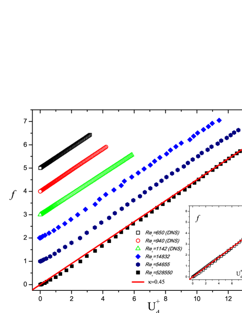
Figure 1: (color). Plot of measured $U^{+}_{d}$ versus theoretical $f(r;r_{c})$ (vertically shift by one) for five sets of data : DNS channel (black and red; $r_{c}=0.27$), DNS pipe (green; $r_{c}=0.23$), experiments pipe (solid diamonds, disks and squares; $r_{c}=0.67$). Note a good linear relation with slope $0.45$ for all Res. The original plot is shown in the inset.

Measurement of $\kappa$ and prediction of the MVP - In the outer flow, $W^{+}\approx\ell_{M}^{+2}S^{+2}\approx r$, which yields $S^{+}\approx\sqrt{r}/\ell_{M}^{+}$. Integrating it using (5) yields an expression for the mean velocity defect, i.e. $U_{d}^{+}=U_{c}^{+}-U^{+}(r)={\mathop{\rm Re}\nolimits}_{\tau}\int_{0}^{r}{S^{+}dr}=(1/\kappa)f(r;r_{c})$, where $U_{c}^{+}$ is the mean velocity at the centreline, and

$$f(r;r_{c})=mZ_{c}\int_{0}^{r}{\frac{{r^{\prime}dr^{\prime}}}{{(1-r^{\prime m})(r^{\prime 2}+r_{c}^{2})^{1/4}}}}=\kappa U_{d}^{+}.$$ (6)

The linear relation between $f(r;r_{c})$ and $U_{d}^{+}$ can be subjected to experimental tests, with a fixed $r_{c}$. In Fig.1, theoretical $f(r;r_{c})$ versus empirical (measured) $U_{d}^{+}$ is plotted for a wide range of data, from direct numerical simulations (DNS) of channel and pipe flow at moderate $Re$ Iwamoto2002 ; Hoyas2006 ; Moin and experiments of pipe flows Mekeon2004 at very high $Re$. The linearity is remarkably observed with a slope of $0.45\pm 0.01$, consistent with our earlier study of channel flows WY2012b . Note that $r_{c}$ can be determined in a rational way, by an evaluation of the minimum relative error, $\sigma_{U}=\frac{1}{N}\sum{\left({1-\kappa U_{d}^{+EXP}(r_{i})/f(r_{i};r_{c})}\right)^{2}}$, where $\kappa$ is the value from the least-square fitting above. In practice, the relative error is evaluated in a domain defined as $200<y^{+}<0.9{\mathop{\rm Re}\nolimits}_{\tau}$. This procedure yields a $r_{c}\approx 2/3$ for Princeton data Mekeon2004 at high $Re_{\tau}>5000$, while at the moderate to low Re, the DNS data Iwamoto2002 ; Hoyas2006 ; Moin show a smaller $r_{c}\approx 0.23\sim 0.27$ for $Re_{\tau}\leq 1000$ (both channel and pipe). With $r_{c}$ so determined, $\kappa$ (i.e. the slope) is measured with high confidence: all data show that $\kappa\approx 0.45$.

This value of $\kappa$ is 10% higher than generally accepted value ($0.41$) Wilcox06 . Initially, it was a bit surprising, but a careful scrutiny confirms the internal consistency of the procedure. Note that in our definition, $\kappa$ is a coefficient defining the outer flow, and its measurement involves little ambiguity. The fact that the measured value is accurately constant for both channel and pipe flows and for a wide range of $Re^{\prime}s$, and that it is exactly the historic Karman constant in the overlap region, suggests that (5) is a better definition for $\kappa$ in channel and pipe flows, and taking into account explicitly the form of the outer flow makes the measurement of $\kappa$ more robust, compared to previous measurements Marusic2010 ; Nagib . Another interesting prediction is an asymptotic centreline dissipation at high $Re$:

$$\varepsilon_{0}^{+Pipe(CH)}=\mathop{\lim}\limits_{r\to 0}(S^{+}W^{+}\Theta)=\frac{{mr_{c}^{3/2}}}{{\kappa Z_{c}^{3}{\mathop{\rm Re}\nolimits}_{\tau}}}\approx\frac{4.6(3.7)}{{\mathop{\rm Re}\nolimits}_{\tau}}.$$ (7)

The constant 3.7 for channel flow becomes 1.18 at $Re_{\tau}\approx 940$ (with $r_{c}\approx 0.27$), which agrees with measured value $\varepsilon_{0}^{+DNS}\approx 1.05/Re_{\tau}$ from DNS data of Hoyas2006 .

In order to predict the MVP, one needs an additional constant. Using (6), we can express the MVP as

$$U^{+}(r)=U^{+}_{c}-f(r;r_{c})/\kappa$$ (8)

Our analysis of the Princeton pipe data at high $Re$ show that $U_{c}^{+}\approx\ln Re_{\tau}/0.45+B_{c}$, with $B_{c}\approx 8.3$. With three parameters: $\kappa\approx 0.45$, $r_{c}\approx 0.67$ and $B_{c}\approx 8.3$, the high-$Re$ outer flow MVP is completely specified by (6) and (8). In addition, an asymptotic calculation of (5) gives $\mathop{\lim}\limits_{r\to 1}f(r;r_{c})=\mathop{\lim}\limits_{r\to 1}\kappa U_{d}^{+}\left(r\right)\approx-\ln\left({1-r}\right)+\kappa B_{d}$ with $B_{d}\approx 1.7$, which only depends on $r_{c}$. Then, (6) yields an approximate log-law in the overlap region:

$$U^{+}(r)\approx\ln y^{+}/0.45+6.6$$ (9)

where the additive constant is found from $B_{c}-B_{d}\approx 8.3-1.7$. In Fig.2, the theoretical MVP (8) is shown to agree with the Princeton pipe data for the entire profile with 99% accuracy for $Re$ up to $4\times 10^{7}$ (better than Lvov2008 ). This unprecedented accuracy settles the debate between the logarithmic law and power law with a rational description of the bulk flow; it further shows that turbulence in pipe flows indeed admits an analytic solution.

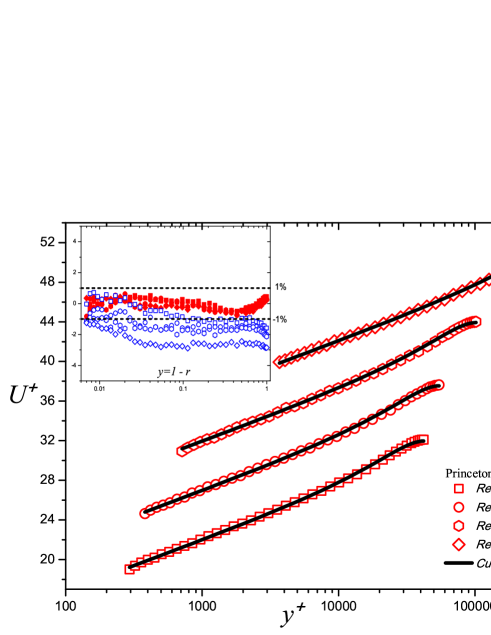
Figure 2: (color). Theoretical (solid lines) and measured MVPs, which are staggered vertically by five units for clarity. Inset shows the relative errors, $(U^{EXP}/U^{THE}-1)\times 100\;\%$ - our predictions (red solid symbols) are uniformly within 1%. Also included (blue open symbols) is the model of L’vov et al. Lvov2008 , which reveals systematic deviations at high $Re$ due to inappropriate boundary constraints WY2012a .

Predictions for fluctuations - The mean kinetic-energy equation (MKE) Pope00 can be rearranged in a form similar to (1) as:

$$-\frac{{dK^{+}}}{{dy^{+}}}+\left\langle{uuv}\right\rangle^{+}=\tau_{K}^{+}$$ (10)

where $K^{+}\equiv\left\langle{uu}\right\rangle^{+}$ is the streamwise kinetic energy, and $\tau_{K}^{+}=\int_{0}^{y^{+}}{(S^{+}W^{+}-\varepsilon^{+}_{K})dy^{+^{\prime}}}-\left\langle{pu}\right\rangle^{+}$ involves the integration of turbulent production, $SW$, dissipation, $\varepsilon_{K}$, and a term due to pressure transport, $\left\langle{pu}\right\rangle^{+}$. Note that one often assumes a quasi-balance, then, $\tau_{K}^{+}$ would be small. Detailed examination of empirical data shows that the integrated deviation from the quasi-balance, although small, is fully responsible for the non-uniform distribution of the kinetic energy.

The similarity between (1) and (10) is a major focus of this paper. Denote $S_{K}^{+}=-dK^{+}/dy^{+}$ and $W_{K}^{+}=\left\langle{uuv}\right\rangle^{+}$, thus, the MKE has a similar form as

$$S_{K}^{+}+W_{K}^{+}=\tau_{K}^{+}.$$ (11)

The two terms on the l.h.s. represent the viscous diffusion and turbulent transport of $K$. Analysis of DNS data of channel flows Hoyas2006 reveals indeed two similarities (results not shown): first, all terms go to zero near the center line, and $W^{+}\sim W^{+}_{K}$ and $S^{+}\sim S^{+}_{K}$; second, $W^{+}_{K}\gg S^{+}_{K}$, but $W^{+}/S^{+}\sim W^{+}_{K}/S^{+}_{K}$. These similarities suggest that (1) and (10) may differ by a constant factor $\alpha$. Assuming this is true, multiplying (1) by $\alpha$ and subtracting (10) yields $d(\alpha U^{+}+K^{+})/dy^{+}\approx 0,$ leading to

$$\alpha U^{+}\left(r\right)+K^{+}\left(r\right)\approx\alpha U_{c}^{+}+K_{c}^{+}\approx C$$ (12)

where $K^{+}_{c}$ is central kinetic energy, with

$$C=(\alpha/\kappa)\ln{Re_{\tau}}+\alpha B_{c}+K^{+}_{c}$$ (13)

being a constant in the outer flow. With experimentally measured $U^{+}(r)$ and $K^{+}(r)$, the validity of (12) is successfully tested (Fig.3) with a $\alpha\approx 0.56$ (Fig.4) by a linear fitting at small $r$ (where the linearity is accurate because both terms have a quadratic dependence on $r$). Fig.3 shows a clear evidence of a spatial invariant over an increasing radial domain with increasing $Re$: the extent reaches almost the entire radius at high $Re$. In addition, the constant $C$ can be measured directly from data at each $Re$, shown in the inset: $C\approx 1.25\ln Re_{\tau}+5.4$. This measurement yields $K^{+}_{c}\approx 0.7$.

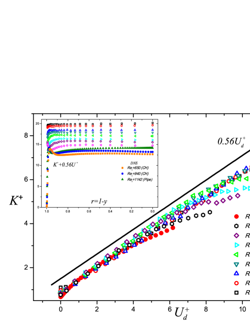
Figure 3: (color). Evidence of linear dependence between $U^{+}_{d}$ and $K^{+}$. The coefficient $\alpha\approx 0.56$ is obtained from fitting the largest $Re$ data. The inset validates the invariance law (12) using experimental $K$ Hulkmark2012 and theoretical $U$ at the same $Re$ with $\alpha$.

A specific prediction of (12) is that at high $Re$, $K$ must have a logarithmic profile (with a negative sign), since $U$ has a logarithmic profile. In the overlap region, $K^{+}\approx-(\alpha/\kappa)\ln y+\alpha B_{d}+K_{c}^{+}\approx-1.25\ln y+1.65$, which reproduces well the empirical observation of Hulkmark et al. Hulkmark2012 : $K^{+}\approx-1.25\ln y+1.61$. Finally, we predict the outer profile of the MKP as

$$K^{+}\approx\alpha f(r;r_{c})/\kappa+K^{+}_{c}.$$ (14)

As shown in Fig.4, it agrees well with empirical data, especially at high $Re$, better than that proposed by Alfredsson et al Alfredsson2011 .

In summary, we have achieved a simultaneous description of the outer MVP and MKP by exploring the similarity in the MME and MKE, which discovers a new spatial invariant in the radius direction of a turbulent pipe. The Lie-group based theory yields a new procedure for measuring $\kappa$ and a universal value of $0.45$ for both channel and pipe flows. The predicted MVPs achieve a 99% accuracy compared to Princeton pipe data for a wide range of $Re^{\prime}s$. Note that the analysis has been successfully extended to incompressible, compressible and rough-wall turbulent boundary layers SED2012a ; SED2012b , and turbulent Rayleigh-Benard convection (temperature). Those results will be communicated soon.

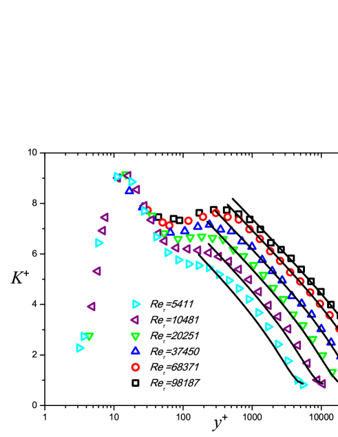
Figure 4: (color). Comparison between the theory (14) (solid lines) and experimental data (symbols) Hulkmark2012 of the MKP.

We thank Y. Wu for helpful discussions. This work is supported by National Nature Science Fund 90716008 and by MOST 973 project 2009CB724100.

$\ast$ Corresponding author. Email: she@pku.edu.cn

References

- (1) D.C. Wilcox, 2006 Turbulence Modeling for CFD. DCW Industries.
- (2) I. Marusic, et al., Phys. Fluids. 22, 065103 (2010).
- (3) A.J. Smits, B.J. McKeon, I. Marusic, Annu. Rev. Fluid Mech. 43, 353-75 (2011).
- (4) V.S. L’vov, et al., Phys. Rev. Lett. 100, 050504 (2008).
- (5) L. Prandtl, Z. Angew. Math. Mech. 5, 136-139 (1925).
- (6) von Karman, In Proc. Third Int. Congr. Applied Mechanics, Stockholm. 85-105.
- (7) G. I. Barenblatt, A. J. Chorin, Proc. Natl Acad. Sci. USA 101, 15023-15026 (2004).
- (8) N. Goldenfeld, Phys. Rev. Lett. 96, 044503 (2006).
- (9) M. Hulkmark, et al., Phys. Rev. Lett. 108, 094501(2012).
- (10) Z.S. She, X. Chen, Y. Wu, F. Hussain, Acta Mech Sinica, 26, 847-861 (2010)
- (11) Z.S. She, X. Chen, F. Hussain, arXiv:1112.6312 (2012)
- (12) L.P. Kadanoff, J. Stat. Phys. 137, 777-797 (2009).
- (13) B.J. McKeon, et al., J. Fluid Mech. 501, 135 (2004)
- (14) S.B. Pope, Turbulent Flows. (Cambridge University Press, Cambridge, 2000).
- (15) K. Iwamoto, Y. Suzuki, N. Kasagi, THTLAB Internal Report. No. ILR-0201 (2002).
- (16) S. Hoyas, J. Jimenez, Phys. Fluids. 18, 011702 (2006).
- (17) X.H. Wu, P. Moin, J. Fluid Mech. 608, 81-112 (2008).
- (18) Y. Wu, X. Chen, Z.S. She and F. Hussain, Physica Scripta, to appear (2012).
- (19) H.M. Nagib, K.A. Chauhan, Phys. Fluids. 20, 101518 (2008).
- (20) Y. Wu, X. Chen, Z.S. She, F. Hussain, Sci China-Phys Mech Astron, 55, 9, 1691-1695 (2012).
- (21) P.H. Alfredsson, et al., Phys. Fluids. 23, 041702 (2011).
- (22) Y.S. Zhang, et al., Phys. Rev. Lett. 109, 054502 (2012).
- (23) Z.S. She, et al., New J. Physics, accepted, (2012).