Abstract
For the first time, we obtain the entropy variation law in a laser process
after finding the Kraus operator of the master equation describing the laser
process with the use of the entangled state representation. The behavior of
entropy is determined by the competition of the gain and damping in the
laser process. The photon number evolution formula is also obtained.
1 Introduction
Since the theoretical foundation proposed by Albert Einstein in 1917 [ 1 ] [ 1 ] {}^{\cite[cite]{[\@@bibref{}{R1}{}{}]}} [ 2 , 3 ] [ 2 , 3 ] {}^{\cite[cite]{[\@@bibref{}{R2,R3}{}{}]}} [ 4 , 5 ] [ 4 , 5 ] {}^{\cite[cite]{[\@@bibref{}{R4,R5}{}{}]}}
In quantum optics theory the time evolution of laser in the lowest-order
approximation can be described by the following master equation of density
operator [ 6 , 7 , 8 , 9 ] [ 6 , 7 , 8 , 9 ] {}^{\cite[cite]{[\@@bibref{}{R6,R7,R8,R9}{}{}]}}
d ρ ( t ) d t = g [ 2 a † ρ ( t ) a − a a † ρ ( t ) − ρ ( t ) a a † ] + κ [ 2 a ρ ( t ) a † − a † a ρ ( t ) − ρ ( t ) a † a ] , 𝑑 𝜌 𝑡 𝑑 𝑡 𝑔 delimited-[] 2 superscript 𝑎 † 𝜌 𝑡 𝑎 𝑎 superscript 𝑎 † 𝜌 𝑡 𝜌 𝑡 𝑎 superscript 𝑎 † 𝜅 delimited-[] 2 𝑎 𝜌 𝑡 superscript 𝑎 † superscript 𝑎 † 𝑎 𝜌 𝑡 𝜌 𝑡 superscript 𝑎 † 𝑎 \begin{array}[]{c}\frac{d\rho\left(t\right)}{dt}=g\left[2a^{\dagger}\rho\left(t\right)a-aa^{\dagger}\rho\left(t\right)-\rho\left(t\right)aa^{\dagger}\right]\\
+\kappa\left[2a\rho\left(t\right)a^{\dagger}-a^{\dagger}a\rho\left(t\right)-\rho\left(t\right)a^{\dagger}a\right],\end{array} (1)
where g 𝑔 g κ 𝜅 \kappa a † , superscript 𝑎 † a^{\dagger}, a 𝑎 a ρ 0 subscript 𝜌 0 \rho_{0} ρ ( t ) 𝜌 𝑡 \rho\left(t\right)
ρ ( t ) = ∑ n = 0 ∞ M n ρ 0 M n † , 𝜌 𝑡 superscript subscript 𝑛 0 subscript 𝑀 𝑛 subscript 𝜌 0 superscript subscript 𝑀 𝑛 † \rho\left(t\right)=\sum_{n=0}^{\infty}M_{n}\rho_{0}M_{n}^{\dagger}, (2)
such an expression is named an operator-sum (Kraus) representation, M n subscript 𝑀 𝑛 M_{n} ρ 0 = | z ⟩ ⟨ z | subscript 𝜌 0 ket 𝑧 bra 𝑧 \rho_{0}=\left|z\right\rangle\left\langle z\right| n 𝑛 n 1
Our way is introducing the two-mode entangled state
| η ⟩ = exp ( − 1 2 | η | 2 + η a † − η ∗ a ~ † + a † a ~ † ) | 0 0 ~ ⟩ , ket 𝜂 1 2 superscript 𝜂 2 𝜂 superscript 𝑎 † superscript 𝜂 ∗ superscript ~ 𝑎 † superscript 𝑎 † superscript ~ 𝑎 † ket 0 ~ 0 |\eta\rangle=\exp(-\frac{1}{2}|\eta|^{2}+\eta a^{{\dagger}}-\eta^{\ast}\tilde{a}^{{\dagger}}+a^{{\dagger}}\tilde{a}^{{\dagger}})|0\tilde{0}\rangle, (3)
where a ~ † superscript ~ 𝑎 † \tilde{a}^{{\dagger}} a † superscript 𝑎 † a^{\dagger} | 0 ~ ⟩ ket ~ 0 |\tilde{0}\rangle a ~ , ~ 𝑎 \tilde{a}, [ a ~ , a ~ † ] = 1 . ~ 𝑎 superscript ~ 𝑎 † 1 \left[\tilde{a},\tilde{a}^{{\dagger}}\right]=1. | η = 0 ⟩ ket 𝜂 0 |\eta=0\rangle
a | η = 0 ⟩ = a ~ † | η = 0 ⟩ , a † | η = 0 ⟩ = a ~ | η = 0 ⟩ , ( a † a ) n | η = 0 ⟩ = ( a ~ † a ~ ) n | η = 0 ⟩ . 𝑎 ket 𝜂 0 superscript ~ 𝑎 † ket 𝜂 0 superscript 𝑎 † ket 𝜂 0 ~ 𝑎 ket 𝜂 0 superscript superscript 𝑎 † 𝑎 𝑛 ket 𝜂 0 superscript superscript ~ 𝑎 † ~ 𝑎 𝑛 ket 𝜂 0 \begin{array}[]{c}a|\eta=0\rangle=\tilde{a}^{{\dagger}}|\eta=0\rangle,\\
a^{{\dagger}}|\eta=0\rangle=\tilde{a}|\eta=0\rangle,\\
(a^{{\dagger}}a)^{n}|\eta=0\rangle=(\tilde{a}^{{\dagger}}\tilde{a})^{n}|\eta=0\rangle.\end{array} (4)
Operating the both sides of (1 | η = 0 ⟩ ≡ | I ⟩ , ket 𝜂 0 ket 𝐼 |\eta=0\rangle\equiv\left|I\right\rangle, | ρ ⟩ = ρ | I ⟩ , ket 𝜌 𝜌 ket 𝐼 \left|\rho\right\rangle=\rho\left|I\right\rangle, 4 | ρ ( t ) ⟩ , ket 𝜌 𝑡 \left|\rho\left(t\right)\right\rangle,
d d t | ρ ( t ) ⟩ = [ g ( 2 a † a ~ † − a a † − a ~ a ~ † ) + κ ( 2 a a ~ − a † a − a ~ † a ~ ) ] | ρ ( t ) ⟩ . 𝑑 𝑑 𝑡 ket 𝜌 𝑡 delimited-[] 𝑔 2 superscript 𝑎 † superscript ~ 𝑎 † 𝑎 superscript 𝑎 † ~ 𝑎 superscript ~ 𝑎 † 𝜅 2 𝑎 ~ 𝑎 superscript 𝑎 † 𝑎 superscript ~ 𝑎 † ~ 𝑎 ket 𝜌 𝑡 \frac{d}{dt}\left|\rho\left(t\right)\right\rangle=\left[\begin{array}[]{c}g\left(2a^{\dagger}\tilde{a}^{\dagger}-aa^{\dagger}-\tilde{a}\tilde{a}^{\dagger}\right)\\
+\kappa\left(2a\tilde{a}-a^{\dagger}a-\tilde{a}^{\dagger}\tilde{a}\right)\end{array}\right]\left|\rho\left(t\right)\right\rangle. (5)
where | ρ 0 ⟩ ≡ ρ 0 | I ⟩ , ket subscript 𝜌 0 subscript 𝜌 0 ket 𝐼 \left|\rho_{0}\right\rangle\equiv\rho_{0}\left|I\right\rangle, ρ 0 subscript 𝜌 0 \rho_{0}
The formal solution of (5
| ρ ( t ) ⟩ = U ( t ) | ρ 0 ⟩ , ket 𝜌 𝑡 𝑈 𝑡 ket subscript 𝜌 0 \left|\rho\left(t\right)\right\rangle=U\left(t\right)\left|\rho_{0}\right\rangle, (6)
and
U ( t ) = exp [ g t ( 2 a † a ~ † − a a † − a ~ a ~ † ) + κ t ( 2 a a ~ − a † a − a ~ † a ~ ) ] . 𝑈 𝑡 𝑔 𝑡 2 superscript 𝑎 † superscript ~ 𝑎 † 𝑎 superscript 𝑎 † ~ 𝑎 superscript ~ 𝑎 † 𝜅 𝑡 2 𝑎 ~ 𝑎 superscript 𝑎 † 𝑎 superscript ~ 𝑎 † ~ 𝑎 U\left(t\right)=\exp\left[\begin{array}[]{c}gt\left(2a^{\dagger}\widetilde{a}^{\dagger}-aa^{\dagger}-\widetilde{a}\widetilde{a}^{\dagger}\right)\\
+\kappa t\left(2a\widetilde{a}-a^{\dagger}a-\widetilde{a}^{\dagger}\widetilde{a}\right)\end{array}\right]. (7)
It challenges us how to disentangle the exponential operator U ( t ) . 𝑈 𝑡 U\left(t\right). U ( t ) 𝑈 𝑡 U\left(t\right)
2 Two Theorems
In order to find the disentangled form of (7 : [ 10 , 11 ] \ {}^{\cite[cite]{[\@@bibref{}{R10,R11}{}{}]}}:
Theorem 1 : The multimode bosonic exponential operator exp ℋ , ℋ \exp\mathcal{H}, ℋ = 1 2 B Γ B ~ , ℋ 1 2 𝐵 Γ ~ 𝐵 \mathcal{H=}\frac{1}{2}B\Gamma\widetilde{B}, B 𝐵 B
B 𝐵 \displaystyle B ≡ \displaystyle\equiv ( A † A ) ≡ ( a 1 † a 2 † ⋯ a n † a 1 a 2 ⋯ a n ) , superscript 𝐴 † 𝐴 superscript subscript 𝑎 1 † superscript subscript 𝑎 2 † ⋯ superscript subscript 𝑎 𝑛 † subscript 𝑎 1 subscript 𝑎 2 ⋯ subscript 𝑎 𝑛 \displaystyle\left(A^{\dagger}\text{ }A\right)\equiv\left(a_{1}^{\dagger}\text{ }a_{2}^{\dagger}\cdot\cdot\cdot\text{ }a_{n}^{\dagger}\text{ }a_{1}\text{\ }a_{2}\cdot\cdot\cdot\text{\ }a_{n}\right), (8)
B ~ ~ 𝐵 \displaystyle\text{ }\widetilde{B} = \displaystyle= ( A ~ † A ~ ) , binomial superscript ~ 𝐴 † ~ 𝐴 \displaystyle\binom{\widetilde{A}^{\dagger}}{\widetilde{A}},
Γ Γ \Gamma 2 n × 2 n 2 𝑛 2 𝑛 2n\times 2n n 𝑛 n
exp ℋ = det Q ∫ ∏ i = 1 n d 2 Z i π | ( Q − L − N P ) ( Z ~ Z ~ ∗ ) ⟩ ⟨ ( Z ~ Z ~ ∗ ) | , ℋ 𝑄 superscript subscript product 𝑖 1 𝑛 superscript 𝑑 2 subscript 𝑍 𝑖 𝜋 ket 𝑄 𝐿 𝑁 𝑃 binomial ~ 𝑍 superscript ~ 𝑍 ∗ bra binomial ~ 𝑍 superscript ~ 𝑍 ∗ \begin{array}[]{c}\exp\mathcal{H}=\sqrt{\det Q}\int\prod\limits_{i=1}^{n}\frac{d^{2}Z_{i}}{\pi}|\left(\begin{array}[]{cc}Q&-L\\
-N&P\end{array}\right)\binom{\widetilde{Z}}{\widetilde{Z}^{\ast}}\rangle\langle\binom{\widetilde{Z}}{\widetilde{Z}^{\ast}}|,\end{array} (9)
where the n 𝑛 n
| ( Z ~ Z ~ ∗ ) ⟩ ket binomial ~ 𝑍 superscript ~ 𝑍 ∗ \displaystyle|\binom{\widetilde{Z}}{\widetilde{Z}^{\ast}}\rangle ≡ \displaystyle\equiv | Z ⟩ = D ( Z ) | 0 → ⟩ , ket 𝑍 𝐷 𝑍 ket → 0
\displaystyle\left|Z\right\rangle=D\left(Z\right)\left|\vec{0}\right\rangle,\text{\ \ } (10)
D ( Z ) 𝐷 𝑍 \displaystyle\text{\ }D\left(Z\right) ≡ \displaystyle\equiv exp { A † Z ~ − A Z ~ ∗ } , superscript 𝐴 † ~ 𝑍 𝐴 superscript ~ 𝑍 ∗ \displaystyle\exp\{A^{\dagger}\widetilde{Z}-A\widetilde{Z}^{\ast}\},
and
( Q L N P ) = exp { Γ Π } , Π = ( 0 − I n I n 0 ) . formulae-sequence 𝑄 𝐿 𝑁 𝑃 Γ Π Π 0 subscript 𝐼 𝑛 subscript 𝐼 𝑛 0 \left(\begin{array}[]{cc}Q&L\\
N&P\end{array}\right)=\exp\{\Gamma\Pi\},\text{ }\Pi=\left(\begin{array}[]{cc}0&-I_{n}\\
I_{n}&0\end{array}\right). (11)
I n subscript 𝐼 𝑛 I_{n} n × n 𝑛 𝑛 n\times n Q , L , N , P 𝑄 𝐿 𝑁 𝑃
Q,L,N,P n × n 𝑛 𝑛 n\times n ( Q L N P ) ≡ M 𝑄 𝐿 𝑁 𝑃 𝑀 \left(\begin{array}[]{cc}Q&L\\
N&P\end{array}\right)\equiv M
M Π M ~ = Π , Π M ~ Π = − M − 1 , formulae-sequence 𝑀 Π ~ 𝑀 Π Π ~ 𝑀 Π superscript 𝑀 1 M\Pi\tilde{M}=\Pi,\text{ }\Pi\tilde{M}\Pi=-M^{-1}, (12)
or
Q L ~ 𝑄 ~ 𝐿 \displaystyle Q\tilde{L} = \displaystyle= L Q ~ , Q P ~ − L N ~ = I , formulae-sequence 𝐿 ~ 𝑄 𝑄 ~ 𝑃 𝐿 ~ 𝑁
𝐼 \displaystyle L\tilde{Q},\text{ }Q\tilde{P}-L\tilde{N}=I,\text{ } (13)
N P ~ 𝑁 ~ 𝑃 \displaystyle\text{ }N\tilde{P} = \displaystyle= P N ~ , P Q ~ − N L ~ = I . 𝑃 ~ 𝑁 𝑃 ~ 𝑄 𝑁 ~ 𝐿
𝐼 \displaystyle P\tilde{N},\text{ }P\tilde{Q}-N\tilde{L}=I.
Theorem 2 : By performing the integration in (9 [ 11 , 12 ] [ 11 , 12 ] {}^{\cite[cite]{[\@@bibref{}{R11,R12}{}{}]}}
exp ℋ = 1 det P exp { − 1 2 A † ( L P − 1 ) A ~ † } × exp { A † ( ln P ~ − 1 ) A ~ } exp { 1 2 A ( P − 1 N ) A ~ } . ℋ 1 𝑃 1 2 superscript 𝐴 † 𝐿 superscript 𝑃 1 superscript ~ 𝐴 † absent superscript 𝐴 † superscript ~ 𝑃 1 ~ 𝐴 1 2 𝐴 superscript 𝑃 1 𝑁 ~ 𝐴 \begin{array}[]{c}\exp\mathcal{H}=\frac{1}{\sqrt{\det P}}\exp\{-\frac{1}{2}A^{\dagger}(LP^{-1})\widetilde{A}^{\dagger}\}\\
\times\exp\{A^{\dagger}(\ln\widetilde{P}^{-1})\widetilde{A}\}\exp\{\frac{1}{2}A(P^{-1}N)\widetilde{A}\}.\end{array} (14)
Now we first appeal to Theorem 1, so we should identify U ( t ) 𝑈 𝑡 U\left(t\right) 7 exp ℋ ℋ \exp\mathcal{H} A = ( a ~ a ) 𝐴 ~ 𝑎 𝑎 A=\left(\begin{array}[]{cc}\widetilde{a}&a\end{array}\right) U ( t ) 𝑈 𝑡 U\left(t\right)
U ( t ) = e ( κ − g ) t exp [ 1 2 B Γ B ~ ] 𝑈 𝑡 superscript 𝑒 𝜅 𝑔 𝑡 1 2 𝐵 Γ ~ 𝐵 U\left(t\right)=e^{\left(\kappa-g\right)t}\exp\left[\frac{1}{2}B\Gamma\widetilde{B}\right] (15)
with Γ Γ \Gamma
Γ = t ( 2 g J 2 − ( g + κ ) I 2 − ( g + κ ) I 2 2 κ J 2 ) Γ 𝑡 2 𝑔 subscript 𝐽 2 𝑔 𝜅 subscript 𝐼 2 𝑔 𝜅 subscript 𝐼 2 2 𝜅 subscript 𝐽 2 \Gamma=t\left(\begin{array}[]{cc}2gJ_{2}&-\left(g+\kappa\right)I_{2}\\
-\left(g+\kappa\right)I_{2}&2\kappa J_{2}\end{array}\right) (16)
here
I 2 = ( 1 0 0 1 ) , J 2 = ( 0 1 1 0 ) , J 2 2 = I 2 , formulae-sequence subscript 𝐼 2 1 0 0 1 formulae-sequence subscript 𝐽 2 0 1 1 0 superscript subscript 𝐽 2 2 subscript 𝐼 2
I_{2}=\left(\begin{array}[]{cc}1&0\\
0&1\end{array}\right),\text{ \ }J_{2}=\left(\begin{array}[]{cc}0&1\\
1&0\end{array}\right),\text{ }J_{2}^{2}=I_{2},\text{ } (17)
we then follow (11 ( Γ Π ) Γ Π \left(\Gamma\Pi\right)
Γ Π = t ( − ( g + κ ) I 2 − 2 g J 2 2 κ J 2 ( g + κ ) I 2 ) Γ Π 𝑡 𝑔 𝜅 subscript 𝐼 2 2 𝑔 subscript 𝐽 2 2 𝜅 subscript 𝐽 2 𝑔 𝜅 subscript 𝐼 2 \Gamma\Pi=t\left(\begin{array}[]{cc}-\left(g+\kappa\right)I_{2}&-2gJ_{2}\\
2\kappa J_{2}&\left(g+\kappa\right)I_{2}\end{array}\right) (18)
therefore
e Γ Π ≡ ( Q L N P ) superscript 𝑒 Γ Π 𝑄 𝐿 𝑁 𝑃 e^{\Gamma\Pi}\equiv\left(\begin{array}[]{cc}Q&L\\
N&P\end{array}\right) (19)
with
Q ≡ g e ( κ − g ) t − κ e ( g − κ ) t g − κ I 2 , L ≡ g [ e ( κ − g ) t − e ( g − κ ) t ] g − κ J 2 , N ≡ κ [ e ( g − κ ) t − e ( κ − g ) t ] g − κ J 2 , P ≡ g e ( g − κ ) t − κ e ( κ − g ) t g − κ I 2 . formulae-sequence 𝑄 𝑔 superscript 𝑒 𝜅 𝑔 𝑡 𝜅 superscript 𝑒 𝑔 𝜅 𝑡 𝑔 𝜅 subscript 𝐼 2 𝐿 𝑔 delimited-[] superscript 𝑒 𝜅 𝑔 𝑡 superscript 𝑒 𝑔 𝜅 𝑡 𝑔 𝜅 subscript 𝐽 2 formulae-sequence 𝑁 𝜅 delimited-[] superscript 𝑒 𝑔 𝜅 𝑡 superscript 𝑒 𝜅 𝑔 𝑡 𝑔 𝜅 subscript 𝐽 2 𝑃 𝑔 superscript 𝑒 𝑔 𝜅 𝑡 𝜅 superscript 𝑒 𝜅 𝑔 𝑡 𝑔 𝜅 subscript 𝐼 2 \begin{array}[]{c}Q\equiv\frac{ge^{\left(\kappa-g\right)t}-\kappa e^{\left(g-\kappa\right)t}}{g-\kappa}I_{2},\text{ }L\equiv\frac{g\left[e^{\left(\kappa-g\right)t}-e^{\left(g-\kappa\right)t}\right]}{g-\kappa}J_{2},\\
N\equiv\frac{\kappa\left[e^{\left(g-\kappa\right)t}-e^{\left(\kappa-g\right)t}\right]}{g-\kappa}J_{2},\text{ }P\equiv\frac{ge^{\left(g-\kappa\right)t}-\kappa e^{\left(\kappa-g\right)t}}{g-\kappa}I_{2}.\end{array} (20)
Thus according to Theorems 1 and 2 we have
U ( t ) = κ − g κ e − 2 ( g − κ ) t − g exp [ g [ 1 − e − 2 ( κ − g ) t ] κ − g e − 2 ( κ − g ) t a ~ † a † ] × exp [ ( a ~ † a ~ + a † a ) ln ( κ − g ) e − ( κ − g ) t κ − g e − 2 ( κ − g ) t ] × exp [ κ [ 1 − e − 2 ( κ − g ) t ] κ − g e − 2 ( κ − g ) t a a ~ ] , 𝑈 𝑡 𝜅 𝑔 𝜅 superscript 𝑒 2 𝑔 𝜅 𝑡 𝑔 𝑔 delimited-[] 1 superscript 𝑒 2 𝜅 𝑔 𝑡 𝜅 𝑔 superscript 𝑒 2 𝜅 𝑔 𝑡 superscript ~ 𝑎 † superscript 𝑎 † absent superscript ~ 𝑎 † ~ 𝑎 superscript 𝑎 † 𝑎 𝜅 𝑔 superscript 𝑒 𝜅 𝑔 𝑡 𝜅 𝑔 superscript 𝑒 2 𝜅 𝑔 𝑡 absent 𝜅 delimited-[] 1 superscript 𝑒 2 𝜅 𝑔 𝑡 𝜅 𝑔 superscript 𝑒 2 𝜅 𝑔 𝑡 𝑎 ~ 𝑎 \begin{array}[]{c}U\left(t\right)=\frac{\kappa-g}{\kappa e^{-2\left(g-\kappa\right)t}-g}\exp\left[\frac{g\left[1-e^{-2\left(\kappa-g\right)t}\right]}{\kappa-ge^{-2\left(\kappa-g\right)t}}\widetilde{a}^{\dagger}a^{\dagger}\right]\\
\times\exp\left[\left(\widetilde{a}^{\dagger}\widetilde{a}+a^{\dagger}a\right)\ln\frac{\left(\kappa-g\right)e^{-\left(\kappa-g\right)t}}{\kappa-ge^{-2\left(\kappa-g\right)t}}\right]\\
\times\exp\left[\frac{\kappa\left[1-e^{-2\left(\kappa-g\right)t}\right]}{\kappa-ge^{-2\left(\kappa-g\right)t}}a\widetilde{a}\right],\end{array} (21)
where we have used
L P − 1 = g [ 1 − e − 2 ( κ − g ) t ] g e − 2 ( κ − g ) t − κ J 2 , P − 1 N = κ [ e − 2 ( κ − g ) t − 1 ] g e − 2 ( κ − g ) t − κ J 2 𝐿 superscript 𝑃 1 𝑔 delimited-[] 1 superscript 𝑒 2 𝜅 𝑔 𝑡 𝑔 superscript 𝑒 2 𝜅 𝑔 𝑡 𝜅 subscript 𝐽 2 superscript 𝑃 1 𝑁 𝜅 delimited-[] superscript 𝑒 2 𝜅 𝑔 𝑡 1 𝑔 superscript 𝑒 2 𝜅 𝑔 𝑡 𝜅 subscript 𝐽 2 \begin{array}[]{c}LP^{-1}=\frac{g\left[1-e^{-2\left(\kappa-g\right)t}\right]}{ge^{-2\left(\kappa-g\right)t}-\kappa}J_{2},\\
P^{-1}N=\frac{\kappa\left[e^{-2\left(\kappa-g\right)t}-1\right]}{ge^{-2\left(\kappa-g\right)t}-\kappa}J_{2}\end{array} (22)
and
det P ≡ g e ( g − κ ) t − κ e ( κ − g ) t g − κ . 𝑃 𝑔 superscript 𝑒 𝑔 𝜅 𝑡 𝜅 superscript 𝑒 𝜅 𝑔 𝑡 𝑔 𝜅 \sqrt{\det P}\equiv\frac{ge^{\left(g-\kappa\right)t}-\kappa e^{\left(\kappa-g\right)t}}{g-\kappa}. (23)
writing
T 1 subscript 𝑇 1 \displaystyle T_{1} = \displaystyle= 1 − e − 2 ( κ − g ) t κ − g e − 2 t ( κ − g ) , T 2 = ( κ − g ) e − ( κ − g ) t κ − g e − 2 t ( κ − g ) , formulae-sequence 1 superscript 𝑒 2 𝜅 𝑔 𝑡 𝜅 𝑔 superscript 𝑒 2 𝑡 𝜅 𝑔 subscript 𝑇 2
𝜅 𝑔 superscript 𝑒 𝜅 𝑔 𝑡 𝜅 𝑔 superscript 𝑒 2 𝑡 𝜅 𝑔 \displaystyle\frac{1-e^{-2\left(\kappa-g\right)t}}{\kappa-ge^{-2t\left(\kappa-g\right)}},\text{ }T_{2}=\frac{\left(\kappa-g\right)e^{-\left(\kappa-g\right)t}}{\kappa-ge^{-2t\left(\kappa-g\right)}},\text{ } (24)
T 3 subscript 𝑇 3 \displaystyle T_{3} = \displaystyle= κ − g κ − g e − 2 t ( κ − g ) = 1 − g T 1 , 𝜅 𝑔 𝜅 𝑔 superscript 𝑒 2 𝑡 𝜅 𝑔 1 𝑔 subscript 𝑇 1 \displaystyle\frac{\kappa-g}{\kappa-ge^{-2t\left(\kappa-g\right)}}=1-gT_{1},
and using (4 6
| ρ ( t ) ⟩ = U ( t ) | ρ 0 ⟩ = T 3 e g T 1 a † a ~ † : e ( T 2 − 1 ) ( a ~ † a ~ + a † a ) : e κ T 1 a a ~ | ρ 0 ⟩ = ∑ i , j = 0 ∞ T 3 κ i g j T 1 i + j i ! j ! T 2 2 j e a † a ln T 2 a † j a i ρ 0 a † i a j e a † a ln T 2 | η = 0 ⟩ , ket 𝜌 𝑡 𝑈 𝑡 ket subscript 𝜌 0 : absent subscript 𝑇 3 superscript 𝑒 𝑔 subscript 𝑇 1 superscript 𝑎 † superscript ~ 𝑎 † superscript 𝑒 subscript 𝑇 2 1 superscript ~ 𝑎 † ~ 𝑎 superscript 𝑎 † 𝑎 : superscript 𝑒 𝜅 subscript 𝑇 1 𝑎 ~ 𝑎 ket subscript 𝜌 0 absent superscript subscript 𝑖 𝑗
0 subscript 𝑇 3 superscript 𝜅 𝑖 superscript 𝑔 𝑗 superscript subscript 𝑇 1 𝑖 𝑗 𝑖 𝑗 superscript subscript 𝑇 2 2 𝑗 superscript 𝑒 superscript 𝑎 † 𝑎 subscript 𝑇 2 superscript 𝑎 † absent 𝑗 superscript 𝑎 𝑖 subscript 𝜌 0 superscript 𝑎 † absent 𝑖 superscript 𝑎 𝑗 superscript 𝑒 superscript 𝑎 † 𝑎 subscript 𝑇 2 ket 𝜂 0 \begin{array}[]{c}\left|\rho\left(t\right)\right\rangle=U\left(t\right)\left|\rho_{0}\right\rangle\\
=T_{3}e^{gT_{1}a^{\dagger}\tilde{a}^{\dagger}}\colon e^{\left(T_{2}-1\right)\left(\tilde{a}^{\dagger}\tilde{a}+a^{\dagger}a\right)}\colon e^{\kappa T_{1}a\tilde{a}}\left|\rho_{0}\right\rangle\\
=\sum\limits_{i,j=0}^{\infty}T_{3}\frac{\kappa^{i}g^{j}T_{1}^{i+j}}{i!j!T_{2}^{2j}}e^{a^{\dagger}a\ln T_{2}}a^{\dagger j}a^{i}\rho_{0}a^{\dagger i}a^{j}e^{a^{\dagger}a\ln T_{2}}\left|\eta=0\right\rangle,\end{array} (25)
or
ρ ( t ) = ∑ i , j = 0 ∞ M i j ρ 0 M i j † , 𝜌 𝑡 superscript subscript 𝑖 𝑗
0 subscript 𝑀 𝑖 𝑗 subscript 𝜌 0 superscript subscript 𝑀 𝑖 𝑗 † \rho\left(t\right)=\sum_{i,j=0}^{\infty}M_{ij}\rho_{0}M_{ij}^{\dagger}, (26)
where
M i j = κ i g j T 3 T 1 i + j i ! j ! T 2 2 j e a † a ln T 2 a † j a i subscript 𝑀 𝑖 𝑗 superscript 𝜅 𝑖 superscript 𝑔 𝑗 subscript 𝑇 3 superscript subscript 𝑇 1 𝑖 𝑗 𝑖 𝑗 superscript subscript 𝑇 2 2 𝑗 superscript 𝑒 superscript 𝑎 † 𝑎 subscript 𝑇 2 superscript 𝑎 † absent 𝑗 superscript 𝑎 𝑖 M_{ij}=\sqrt{\frac{\kappa^{i}g^{j}T_{3}T_{1}^{i+j}}{i!j!T_{2}^{2j}}}e^{a^{\dagger}a\ln T_{2}}a^{\dagger j}a^{i} (27)
is the Kraus operator, and one can check
∑ i , j = 0 ∞ M i j † M i j = 1 . superscript subscript 𝑖 𝑗
0 superscript subscript 𝑀 𝑖 𝑗 † subscript 𝑀 𝑖 𝑗 1 \sum_{i,j=0}^{\infty}M_{ij}^{\dagger}M_{ij}=1. (28)
3 The Photon Number Evolution
Now we have an explicit solution of the density matrix of a laser (26 ρ 0 = | z ⟩ ⟨ z | subscript 𝜌 0 ket 𝑧 bra 𝑧 \rho_{0}=\left|z\right\rangle\left\langle z\right| | z ⟩ = exp [ − | z | 2 / 2 + z a † ] | 0 ⟩ , ket 𝑧 superscript 𝑧 2 2 𝑧 superscript 𝑎 † ket 0 \ \left|z\right\rangle=\exp[-|z|^{2}/2+za^{\dagger}]\left|0\right\rangle,
⟨ n ⟩ = T r [ ρ ( t ) a † a ] = e κ T 1 | z | 2 T r [ ∑ j = 0 ∞ T 3 g j T 1 j j ! T 2 2 j e a † a ln T 2 a † j | z ⟩ ⟨ z | a j e a † a ln T 2 a † a ] delimited-⟨⟩ 𝑛 𝑇 𝑟 delimited-[] 𝜌 𝑡 superscript 𝑎 † 𝑎 absent superscript 𝑒 𝜅 subscript 𝑇 1 superscript 𝑧 2 𝑇 𝑟 delimited-[] superscript subscript 𝑗 0 subscript 𝑇 3 superscript 𝑔 𝑗 superscript subscript 𝑇 1 𝑗 𝑗 superscript subscript 𝑇 2 2 𝑗 superscript 𝑒 superscript 𝑎 † 𝑎 subscript 𝑇 2 superscript 𝑎 † absent 𝑗 ket 𝑧 bra 𝑧 superscript 𝑎 𝑗 superscript 𝑒 superscript 𝑎 † 𝑎 subscript 𝑇 2 superscript 𝑎 † 𝑎 \begin{array}[]{c}\left\langle n\right\rangle=Tr\left[\rho\left(t\right)a^{\dagger}a\right]\\
=e^{\kappa T_{1}\left|z\right|^{2}}Tr\left[\sum\limits_{j=0}^{\infty}T_{3}\frac{g^{j}T_{1}^{j}}{j!T_{2}^{2j}}e^{a^{\dagger}a\ln T_{2}}a^{\dagger j}\left|z\right\rangle\left\langle z\right|a^{j}e^{a^{\dagger}a\ln T_{2}}a^{\dagger}a\right]\end{array} (29)
Then using | 0 ⟩ ⟨ 0 | = : e − a † a : , \left|0\right\rangle\left\langle 0\right|=:e^{-a^{\dagger}a}:, ∫ d 2 z π | z ⟩ ⟨ z | = 1 superscript 𝑑 2 𝑧 𝜋 ket 𝑧 bra 𝑧 1 \int\frac{d^{2}z}{\pi}\left|z\right\rangle\left\langle z\right|=1
⟨ n ⟩ = T 3 e ( κ T 1 − 1 ) | z | 2 T r [ ∑ j = 0 ∞ g j T 1 j j ! a † j e z T 2 a † : e − a † a : e z ∗ T 2 a a j a † a ] = T 3 e ( κ T 1 − 1 ) | z | 2 T r [ e z T 2 a † e a † a ln ( g T 1 ) e z ∗ T 2 a a † a ] = T 3 e ( κ T 1 − 1 ) | z | 2 T r [ e z T 2 a † ( g T 1 a † + z ∗ T 2 ) e a † a ln ( g T 1 ) e z ∗ T 2 a a ] = T 3 e ( κ T 1 − 1 ) | z | 2 ∫ d 2 z ′ π ⟨ z ′ | × : e z T 2 a † + z ∗ T 2 a + ( g T 1 − 1 ) a † a ( g T 1 a † + z ∗ T 2 ) a : | z ′ ⟩ = g 1 − e − 2 ( κ − g ) t κ − g + | z | 2 e − 2 ( κ − g ) t . \begin{array}[]{c}\left\langle n\right\rangle\\
=T_{3}e^{\left(\kappa T_{1}-1\right)\left|z\right|^{2}}Tr\left[\sum\limits_{j=0}^{\infty}\frac{g^{j}T_{1}^{j}}{j!}a^{\dagger j}e^{zT_{2}a^{\dagger}}:e^{-a^{\dagger}a}:e^{z^{\ast}T_{2}a}a^{j}a^{\dagger}a\right]\\
=T_{3}e^{\left(\kappa T_{1}-1\right)\left|z\right|^{2}}Tr\left[e^{zT_{2}a^{\dagger}}e^{a^{\dagger}a\ln\left(gT_{1}\right)}e^{z^{\ast}T_{2}a}a^{\dagger}a\right]\\
=T_{3}e^{\left(\kappa T_{1}-1\right)\left|z\right|^{2}}Tr\left[e^{zT_{2}a^{\dagger}}\left(gT_{1}a^{\dagger}+z^{\ast}T_{2}\right)e^{a^{\dagger}a\ln\left(gT_{1}\right)}e^{z^{\ast}T_{2}a}a\right]\\
=T_{3}e^{\left(\kappa T_{1}-1\right)\left|z\right|^{2}}\int\frac{d^{2}z^{\prime}}{\pi}\left\langle z^{\prime}\right|\\
\times:e^{zT_{2}a^{\dagger}+z^{\ast}T_{2}a+\left(gT_{1}-1\right)a^{\dagger}a}\left(gT_{1}a^{\dagger}+z^{\ast}T_{2}\right)a:\left|z^{\prime}\right\rangle\\
=g\frac{1-e^{-2\left(\kappa-g\right)t}}{\kappa-g}+\left|z\right|^{2}e^{-2\left(\kappa-g\right)t}.\end{array} (30)
We can easily write down the asymptotic behavior of ⟨ n ⟩ delimited-⟨⟩ 𝑛 \left\langle n\right\rangle t → + ∞ → 𝑡 t\rightarrow+\infty
If κ = g 𝜅 𝑔 \kappa=g ⟨ n ⟩ = | z | 2 + 2 g t delimited-⟨⟩ 𝑛 superscript 𝑧 2 2 𝑔 𝑡 \left\langle n\right\rangle=\left|z\right|^{2}+2gt
If κ < g 𝜅 𝑔 \kappa<g ⟨ n ⟩ ∼ ( g g − κ + | z | 2 ) e 2 ( g − κ ) t similar-to delimited-⟨⟩ 𝑛 𝑔 𝑔 𝜅 superscript 𝑧 2 superscript 𝑒 2 𝑔 𝜅 𝑡 \left\langle n\right\rangle\sim\left(\frac{g}{g-\kappa}+\left|z\right|^{2}\right)e^{2\left(g-\kappa\right)t} t → + ∞ . → 𝑡 t\rightarrow+\infty.
If κ > g 𝜅 𝑔 \kappa>g ⟨ n ⟩ ∼ g κ − g similar-to delimited-⟨⟩ 𝑛 𝑔 𝜅 𝑔 \left\langle n\right\rangle\sim\frac{g}{\kappa-g} t → + ∞ . → 𝑡 t\rightarrow+\infty.
4
We now calculate how the entropy of a laser evolves with time. Using (26 ρ ( t ) 𝜌 𝑡 \rho\left(t\right) | z ⟩ ⟨ z | ket 𝑧 bra 𝑧 \left|z\right\rangle\left\langle z\right|
ρ ( t ) = T 3 exp [ | z | 2 e 2 ( g − κ ) t ln g T 1 ] × ∑ j = 0 ∞ g j T 1 j j ! T 2 2 j : a † j a j e z a † + z ∗ a − a † a : e a † a ln T 2 = T 3 e κ T 1 | z | 2 − | z | 2 e z T 2 a † e a † a ln ( g T 1 ) e z ∗ T 2 a . \begin{array}[]{c}\rho\left(t\right)=T_{3}\exp\left[\left|z\right|^{2}e^{2\left(g-\kappa\right)t}\ln gT_{1}\right]\\
\times\sum\limits_{j=0}^{\infty}\frac{g^{j}T_{1}^{j}}{j!T_{2}^{2j}}:a^{\dagger j}a^{j}e^{za^{\dagger}+z^{\ast}a-a^{\dagger}a}:e^{a^{\dagger}a\ln T_{2}}\\
=T_{3}e^{\kappa T_{1}\left|z\right|^{2}-\left|z\right|^{2}}e^{zT_{2}a^{\dagger}}e^{a^{\dagger}a\ln\left(gT_{1}\right)}e^{z^{\ast}T_{2}a}.\end{array} (31)
By the Baker–Campbell–Hausdorff formula, if
[ X , Y ] = λ Y + μ , 𝑋 𝑌 𝜆 𝑌 𝜇 \left[X,Y\right]=\lambda Y+\mu, (32)
then
exp X exp Y = exp ( X + λ Y + μ 1 − e − λ − μ λ ) . 𝑋 𝑌 𝑋 𝜆 𝑌 𝜇 1 superscript 𝑒 𝜆 𝜇 𝜆 \exp X\exp Y=\exp\left(X+\frac{\lambda Y+\mu}{1-e^{-\lambda}}-\frac{\mu}{\lambda}\right). (33)
we can compact the three exponentials in (31
ρ ( t ) = T 3 exp [ | z | 2 e 2 ( g − κ ) t ln g T 1 ] × exp { [ a † a − e ( g − κ ) t ( z a † + z ∗ a ) ] ln g T 1 } . 𝜌 𝑡 subscript 𝑇 3 superscript 𝑧 2 superscript 𝑒 2 𝑔 𝜅 𝑡 𝑔 subscript 𝑇 1 absent delimited-[] superscript 𝑎 † 𝑎 superscript 𝑒 𝑔 𝜅 𝑡 𝑧 superscript 𝑎 † superscript 𝑧 ∗ 𝑎 𝑔 subscript 𝑇 1 \begin{array}[]{c}\rho\left(t\right)=T_{3}\exp\left[\left|z\right|^{2}e^{2\left(g-\kappa\right)t}\ln gT_{1}\right]\\
\times\exp\left\{\left[a^{\dagger}a-e^{\left(g-\kappa\right)t}\left(za^{\dagger}+z^{\ast}a\right)\right]\ln gT_{1}\right\}.\end{array} (34)
with direct calculations. Thus we see how a pure state | z ⟩ ⟨ z | ket 𝑧 bra 𝑧 \left|z\right\rangle\left\langle z\right| 3 ρ ( t ) 𝜌 𝑡 \rho\left(t\right)
ln ρ ( t ) = ln T 3 + | z | 2 e 2 ( g − κ ) t ln g T 1 + [ a † a − e ( g − κ ) t ( z a † + z ∗ a ) ] ln g T 1 . 𝜌 𝑡 subscript 𝑇 3 superscript 𝑧 2 superscript 𝑒 2 𝑔 𝜅 𝑡 𝑔 subscript 𝑇 1 delimited-[] superscript 𝑎 † 𝑎 superscript 𝑒 𝑔 𝜅 𝑡 𝑧 superscript 𝑎 † superscript 𝑧 ∗ 𝑎 𝑔 subscript 𝑇 1 \begin{array}[]{c}\ln\rho\left(t\right)=\ln T_{3}+\left|z\right|^{2}e^{2\left(g-\kappa\right)t}\ln gT_{1}\\
+\left[a^{\dagger}a-e^{\left(g-\kappa\right)t}\left(za^{\dagger}+z^{\ast}a\right)\right]\ln gT_{1}.\end{array} (35)
Therefore the von-Neumann entropy of ρ ( t ) 𝜌 𝑡 \rho\left(t\right)
S ( ρ ( t ) ) / k B = − T r [ ρ ln ρ ] = − T r [ ρ ( ln T 3 + | z | 2 e 2 ( g − κ ) t ln g T 1 ) ] − T 3 e ( κ T 1 − 1 ) | z | 2 ln g T 1 × T r [ e z T 2 a † e a † a ln g T 1 e z ∗ T 2 a ( a † a − e ( g − κ ) t ( z a † + z ∗ a ) ) ] = − ln T 3 − | z | 2 e 2 ( g − κ ) t ln g T 1 − T 3 e ( κ T 1 − 1 ) | z | 2 ln g T 1 × T r [ e z T 2 a † e a † a ln g T 1 e z ∗ T 2 a ( a † a − e ( g − κ ) t ( z a † + z ∗ a ) ) ] , 𝑆 𝜌 𝑡 subscript 𝑘 𝐵 𝑇 𝑟 delimited-[] 𝜌 𝜌 absent 𝑇 𝑟 delimited-[] 𝜌 subscript 𝑇 3 superscript 𝑧 2 superscript 𝑒 2 𝑔 𝜅 𝑡 𝑔 subscript 𝑇 1 subscript 𝑇 3 superscript 𝑒 𝜅 subscript 𝑇 1 1 superscript 𝑧 2 𝑔 subscript 𝑇 1 absent 𝑇 𝑟 delimited-[] superscript 𝑒 𝑧 subscript 𝑇 2 superscript 𝑎 † superscript 𝑒 superscript 𝑎 † 𝑎 𝑔 subscript 𝑇 1 superscript 𝑒 superscript 𝑧 ∗ subscript 𝑇 2 𝑎 superscript 𝑎 † 𝑎 superscript 𝑒 𝑔 𝜅 𝑡 𝑧 superscript 𝑎 † superscript 𝑧 ∗ 𝑎 absent subscript 𝑇 3 superscript 𝑧 2 superscript 𝑒 2 𝑔 𝜅 𝑡 𝑔 subscript 𝑇 1 subscript 𝑇 3 superscript 𝑒 𝜅 subscript 𝑇 1 1 superscript 𝑧 2 𝑔 subscript 𝑇 1 absent 𝑇 𝑟 delimited-[] superscript 𝑒 𝑧 subscript 𝑇 2 superscript 𝑎 † superscript 𝑒 superscript 𝑎 † 𝑎 𝑔 subscript 𝑇 1 superscript 𝑒 superscript 𝑧 ∗ subscript 𝑇 2 𝑎 superscript 𝑎 † 𝑎 superscript 𝑒 𝑔 𝜅 𝑡 𝑧 superscript 𝑎 † superscript 𝑧 ∗ 𝑎 \begin{array}[]{c}S\left(\rho\left(t\right)\right)/k_{B}=-Tr\left[\rho\ln\rho\right]\\
=-Tr\left[\rho\left(\ln T_{3}+\left|z\right|^{2}e^{2\left(g-\kappa\right)t}\ln gT_{1}\right)\right]-T_{3}e^{\left(\kappa T_{1}-1\right)\left|z\right|^{2}}\ln gT_{1}\\
\times Tr\left[e^{zT_{2}a^{\dagger}}e^{a^{\dagger}a\ln gT_{1}}e^{z^{\ast}T_{2}a}\left(a^{\dagger}a-e^{\left(g-\kappa\right)t}\left(za^{\dagger}+z^{\ast}a\right)\right)\right]\\
=-\ln T_{3}-\left|z\right|^{2}e^{2\left(g-\kappa\right)t}\ln gT_{1}-T_{3}e^{\left(\kappa T_{1}-1\right)\left|z\right|^{2}}\ln gT_{1}\\
\times Tr\left[e^{zT_{2}a^{\dagger}}e^{a^{\dagger}a\ln gT_{1}}e^{z^{\ast}T_{2}a}\left(a^{\dagger}a-e^{\left(g-\kappa\right)t}\left(za^{\dagger}+z^{\ast}a\right)\right)\right],\end{array} (36)
where k B subscript 𝑘 𝐵 k_{B}
e z T 2 a † e a † a ln g T 1 e z ∗ T 2 a [ a † a − e ( g − κ ) t z a † ] = e z T 2 a † e a † a ln g T 1 ( a † + z ∗ T 2 ) e z ∗ T 2 a a − e ( g − κ ) t z e z T 2 a † e a † a ln g T 1 ( a † + z ∗ T 2 ) e z ∗ T 2 a = e z T 2 a † ( g T 1 a † + z ∗ T 2 ) e a † a ln g T 1 e z ∗ T 2 a a − e ( g − κ ) t z e z T 2 a † ( g T 1 a † + z ∗ T 2 ) e a † a ln g T 1 e z ∗ T 2 a , superscript 𝑒 𝑧 subscript 𝑇 2 superscript 𝑎 † superscript 𝑒 superscript 𝑎 † 𝑎 𝑔 subscript 𝑇 1 superscript 𝑒 superscript 𝑧 ∗ subscript 𝑇 2 𝑎 delimited-[] superscript 𝑎 † 𝑎 superscript 𝑒 𝑔 𝜅 𝑡 𝑧 superscript 𝑎 † absent superscript 𝑒 𝑧 subscript 𝑇 2 superscript 𝑎 † superscript 𝑒 superscript 𝑎 † 𝑎 𝑔 subscript 𝑇 1 superscript 𝑎 † superscript 𝑧 ∗ subscript 𝑇 2 superscript 𝑒 superscript 𝑧 ∗ subscript 𝑇 2 𝑎 𝑎 superscript 𝑒 𝑔 𝜅 𝑡 𝑧 superscript 𝑒 𝑧 subscript 𝑇 2 superscript 𝑎 † superscript 𝑒 superscript 𝑎 † 𝑎 𝑔 subscript 𝑇 1 superscript 𝑎 † superscript 𝑧 ∗ subscript 𝑇 2 superscript 𝑒 superscript 𝑧 ∗ subscript 𝑇 2 𝑎 absent superscript 𝑒 𝑧 subscript 𝑇 2 superscript 𝑎 † 𝑔 subscript 𝑇 1 superscript 𝑎 † superscript 𝑧 ∗ subscript 𝑇 2 superscript 𝑒 superscript 𝑎 † 𝑎 𝑔 subscript 𝑇 1 superscript 𝑒 superscript 𝑧 ∗ subscript 𝑇 2 𝑎 𝑎 superscript 𝑒 𝑔 𝜅 𝑡 𝑧 superscript 𝑒 𝑧 subscript 𝑇 2 superscript 𝑎 † 𝑔 subscript 𝑇 1 superscript 𝑎 † superscript 𝑧 ∗ subscript 𝑇 2 superscript 𝑒 superscript 𝑎 † 𝑎 𝑔 subscript 𝑇 1 superscript 𝑒 superscript 𝑧 ∗ subscript 𝑇 2 𝑎 \begin{array}[]{c}e^{zT_{2}a^{\dagger}}e^{a^{\dagger}a\ln gT_{1}}e^{z^{\ast}T_{2}a}\left[a^{\dagger}a-e^{\left(g-\kappa\right)t}za^{\dagger}\right]\\
=e^{zT_{2}a^{\dagger}}e^{a^{\dagger}a\ln gT_{1}}\left(a^{\dagger}+z^{\ast}T_{2}\right)e^{z^{\ast}T_{2}a}a\\
-e^{\left(g-\kappa\right)t}ze^{zT_{2}a^{\dagger}}e^{a^{\dagger}a\ln gT_{1}}\left(a^{\dagger}+z^{\ast}T_{2}\right)e^{z^{\ast}T_{2}a}\\
=e^{zT_{2}a^{\dagger}}\left(gT_{1}a^{\dagger}+z^{\ast}T_{2}\right)e^{a^{\dagger}a\ln gT_{1}}e^{z^{\ast}T_{2}a}a\\
-e^{\left(g-\kappa\right)t}ze^{zT_{2}a^{\dagger}}\left(gT_{1}a^{\dagger}+z^{\ast}T_{2}\right)e^{a^{\dagger}a\ln gT_{1}}e^{z^{\ast}T_{2}a},\end{array} (37)
therefore
T r [ e z T 2 a † e a † a ln g T 1 e z ∗ T 2 a z ∗ T 2 a ( a † a − e ( g − κ ) t ( z a † + z ∗ a ) ) ] = ∫ d 2 z ′ π ⟨ z ′ | : e z T 2 a † + z ∗ T 2 a + ( g T 1 − 1 ) a † a × [ ( g T 1 a † + z ∗ T 2 ) ( a − e ( g − κ ) t z ) − e ( g − κ ) t z ∗ a ] : | z ′ ⟩ = ∫ d 2 z ′ π e z T 2 z ′ ∗ + z ∗ T 2 z ′ + ( g T 1 − 1 ) | z ′ | 2 × [ ( g T 1 z ′ ∗ + z ∗ T 2 ) ( z ′ − e ( g − κ ) t z ) − e ( g − κ ) t z ∗ z ′ ] . \begin{array}[]{c}Tr\left[e^{zT_{2}a^{\dagger}}e^{a^{\dagger}a\ln gT_{1}}e^{z^{\ast}T_{2}az^{\ast}T_{2}a}\left(a^{\dagger}a-e^{\left(g-\kappa\right)t}\left(za^{\dagger}+z^{\ast}a\right)\right)\right]\\
=\int\frac{d^{2}z^{\prime}}{\pi}\left\langle z^{\prime}\right|:e^{zT_{2}a^{\dagger}+z^{\ast}T_{2}a+\left(gT_{1}-1\right)a^{\dagger}a}\\
\times\left[\left(gT_{1}a^{\dagger}+z^{\ast}T_{2}\right)\left(a-e^{\left(g-\kappa\right)t}z\right)-e^{\left(g-\kappa\right)t}z^{\ast}a\right]:\left|z^{\prime}\right\rangle\\
=\int\frac{d^{2}z^{\prime}}{\pi}e^{zT_{2}z^{\prime\ast}+z^{\ast}T_{2}z^{\prime}+\left(gT_{1}-1\right)\left|z^{\prime}\right|^{2}}\\
\times\left[\left(gT_{1}z^{\prime\ast}+z^{\ast}T_{2}\right)\left(z^{\prime}-e^{\left(g-\kappa\right)t}z\right)-e^{\left(g-\kappa\right)t}z^{\ast}z^{\prime}\right].\end{array} (38)
Finally the entropy variation law is
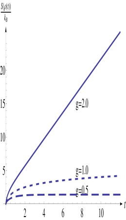
S ( ρ ( t ) ) = − k B ( ln T 3 + g T 1 ln g T 1 1 − g T 1 ) 𝑆 𝜌 𝑡 subscript 𝑘 𝐵 subscript 𝑇 3 𝑔 subscript 𝑇 1 𝑔 subscript 𝑇 1 1 𝑔 subscript 𝑇 1 S\left(\rho\left(t\right)\right)=-k_{B}\left(\ln T_{3}+\frac{gT_{1}\ln gT_{1}}{1-gT_{1}}\right) (39)
Figure 1: S ( ρ ( t ) ) / k B 𝑆 𝜌 𝑡 subscript 𝑘 𝐵 S\left(\rho\left(t\right)\right)/k_{B} for z = 4 , κ = 1 formulae-sequence 𝑧 4 𝜅 1 z=4,\kappa=1 g = 2 , 1 , 0.5 𝑔 2 1 0.5
g=2,1,0.5
We also write down the asymptotic behavior of S ( ρ ( t ) ) 𝑆 𝜌 𝑡 S\left(\rho\left(t\right)\right) t → + ∞ → 𝑡 t\rightarrow+\infty
If κ = g 𝜅 𝑔 \kappa=g S ( ρ ( t ) ) / k B ∼ similar-to 𝑆 𝜌 𝑡 subscript 𝑘 𝐵 absent S\left(\rho\left(t\right)\right)/k_{B}\sim 1 + ln ( 2 g t ) 1 2 𝑔 𝑡 1+\ln\left(2gt\right) t → + ∞ → 𝑡 t\rightarrow+\infty
If κ < g 𝜅 𝑔 \kappa<g S ( ρ ( t ) ) / k B ∼ 1 + ln g g − κ + 2 ( g − κ ) t similar-to 𝑆 𝜌 𝑡 subscript 𝑘 𝐵 1 𝑔 𝑔 𝜅 2 𝑔 𝜅 𝑡 S\left(\rho\left(t\right)\right)/k_{B}\sim 1+\ln\frac{g}{g-\kappa}+2\left(g-\kappa\right)t t → + ∞ → 𝑡 t\rightarrow+\infty
If κ > g 𝜅 𝑔 \kappa>g S ( ρ ( t ) ) / k B ∼ ln κ κ − g + g κ − g ln κ g similar-to 𝑆 𝜌 𝑡 subscript 𝑘 𝐵 𝜅 𝜅 𝑔 𝑔 𝜅 𝑔 𝜅 𝑔 S\left(\rho\left(t\right)\right)/k_{B}\sim\ln\frac{\kappa}{\kappa-g}+\frac{g}{\kappa-g}\ln\frac{\kappa}{g} t → + ∞ → 𝑡 t\rightarrow+\infty
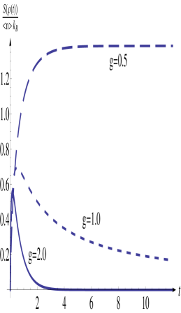
The results of expected photon number and entropy of the laser do not depend on the phase of parameter z 𝑧 z z 𝑧 z z 𝑧 z
Plots of S ( ρ ( t ) ) 𝑆 𝜌 𝑡 S\left(\rho\left(t\right)\right) S ( ρ ( t ) ) ⟨ n ⟩ 𝑆 𝜌 𝑡 delimited-⟨⟩ 𝑛 \frac{S\left(\rho\left(t\right)\right)}{\left\langle n\right\rangle} k B subscript 𝑘 𝐵 k_{B} z = 4 𝑧 4 z=4 , κ = 1 𝜅 1 \kappa=1 g = 2 , 1 , 0.5 𝑔 2 1 0.5
g=2,1,0.5 g 𝑔 g κ 𝜅 \kappa T = ℏ ω k B ln κ g 𝑇 Planck-constant-over-2-pi 𝜔 subscript 𝑘 𝐵 𝜅 𝑔 T=\frac{\hbar\omega}{k_{B}}\ln\frac{\kappa}{g} g 𝑔 g κ 𝜅 \kappa g 𝑔 g
Figure 2: S ( ρ ( t ) ) / ( ⟨ n ⟩ k B ) 𝑆 𝜌 𝑡 delimited-⟨⟩ 𝑛 subscript 𝑘 𝐵 S\left(\rho\left(t\right)\right)/{(\langle n\rangle k_{B})} for z = 4 , κ = 1 formulae-sequence 𝑧 4 𝜅 1 z=4,\kappa=1 g = 2 , 1 , 0.5 𝑔 2 1 0.5
g=2,1,0.5