Exotic symmetry and monodromy equivalence in Schrödinger sigma models

Abstract

We consider the classical integrable structure of two-dimensional non-linear sigma models with target space three-dimensional Schrödinger spacetimes. There are the two descriptions to describe the classical dynamics: 1) the left description based on $SL(2,\mathbb{R})_{\rm L}$ and 2) the right description based on $U(1)_{\rm R}$ . We have shown the $sl(2,{\mathbb{R}})_{\rm L}$ Yangian and $q$-deformed Poincaré algebras associated with them. We proceed to argue an infinite-dimensional extension of the $q$-deformed Poincaré algebra. The corresponding charges are constructed by using a non-local map from the flat conserved currents related to the Yangian. The exotic tower structure of the charges is revealed by directly computing the classical Poisson brackets. Then the monodromy matrices in both descriptions are shown to be gauge-equivalent via the relation between the spectral parameters. We also give a simple Riemann sphere interpretation of this equivalence.

1 Introduction

In the recent studies of the AdS/CFT correspondence M ; GKP ; W , Schrödinger spacetimes Son ; BM have been in the spotlight. The spacetimes are basically null-deformations of the usual AdS spaces and the relativistic conformal algebra is broken to a subalgebra called the Schrödinger algebra Sch1 ; Sch2 . Those are considered to be holographic dual to non-relativistic (NR) CFTs Henkel ; Nishida realized by using ultra cold atoms in real laboratories. This observation is of great significance because it might be possible to test string theory from tabletop experiments (for reviews see Lecture1 ; Lecture2 ).

To elaborate the AdS/NRCFT correspondence, it is interesting to explore the integrability of two-dimensional non-linear sigma models with target space Schrödinger spacetimes. The integrability in AdS/CFT has played an important role in studying the matching of the spectra (for a comprehensive review see review ). The integrability yields a powerful tool to examine AdS/NRCFT as well.

Schrödinger spacetimes are represented by non-symmetric and non-reductive cosets SYY , hence the classical integrable structure is far from obvious. Although the integrability has not been clarified in more than three dimensions so far, the sigma models on three-dimensional Schrödinger spacetimes are shown to be classically integrable by explicitly constructing an infinite set of non-local charges and showing that the classical $r/s$-matrices satisfy the extended Yang-Baxter equation KY-Sch . Thus the spacetimes are regarded as integrable deformations of AdS₃ . An intensive analysis on other integrable deformations has been done in the recent work BR .

In this paper we proceed our previous analysis on the classical integrable structure of two-dimensional non-linear sigma models on three-dimensional Schrödinger spacetimes KY-Sch . There are the two descriptions to describe the classical dynamics: 1) the left description based on $SL(2,\mathbb{R})_{\rm L}$ and 2) the right description based on $U(1)_{\rm R}$ . We have shown the $sl(2,{\mathbb{R}})_{\rm L}$ Yangian and $q$-deformed Poincaré algebras associated with them KY-Sch . However, while the Yangian is an infinite-dimensional symmetry, the $q$-deformed Poincaré symmetry is finite-dimensional.

The main purpose here is to argue an infinite-dimensional extension of the $q$-deformed Poincaré algebra. The corresponding charges are constructed by using a non-local map from the flat conserved currents related to the Yangian. The exotic tower structure of the charges is revealed by directly computing the classical Poisson brackets. Then the monodromy matrices in both descriptions are shown to be gauge-equivalent via the relation between the spectral parameters. We also give a simple Riemann sphere interpretation of this equivalence.

This paper is organized as follows. In section 2 we introduce the classical action of two-dimensional non-linear sigma models on three-dimensional Schrödinger spacetimes. In section 3 the left description based on $SL(2,{\mathbb{R}})_{\rm L}$ is revisited. We carefully reconsider the flat conserved currents, focusing upon the sign of the current improvement. In section 4 our previous analysis on the right description based on $U(1)_{\rm R}$ further proceeds. An infinite-dimensional extension of $q$-deformed Poincaré algebra is shown directly by constructing the conserved charges. The tower structure of the charges is generated in an exotic way. Then we show the gauge-equivalence of the monodromy matrices in the two descriptions and give a simple Riemann sphere interpretation of it. Section 5 is devoted to conclusion and discussion. In appendix A we show the right current algebra that is used to compute the algebra of non-local conserved charges in section 4. In appendix B we explain in detail the prescription utilized in computing the algebra of an infinite dimensional extension of the $q$-deformed Poincaré algebra.

2 Setup

In this section we introduce the classical action of two-dimensional non-linear sigma models on three-dimensional Schrödinger spacetimes

2.1 Schrödinger spacetimes

Schrödinger spacetimes in three dimensions are known as null-like deformations of AdS₃ . And the metric of the spacetimes is given by

$$ds^{2}=L^{2}\left[-2{\rm e}^{-2\rho}dudv+d\rho^{2}-C{\rm e}^{-4\rho}dv^{2}\right]\,.$$ (1)

The deformation is measured by a real constant parameter $C$ . When $C=0$ , the metric (1) describes the AdS₃ space with the curvature radius $L$ and the isometry is $SO(2,2)=SL(2,{\mathbb{R}})_{\rm L}\times SL(2,{\mathbb{R}})_{\rm R}$ . When $C\neq 0$ , the $SL(2,{\mathbb{R}})_{\rm R}$ symmetry is broken to $U(1)_{\rm R}$ while the $SL(2,{\mathbb{R}})_{\rm L}$ symmetry is preserved. Hence the symmetry that survives the deformation is $SL(2,{\mathbb{R}})_{\rm L}\times U(1)_{\rm R}$ in total. This symmetry yields two distinct descriptions to describe the classical dynamics as we will see later.

It is useful to rewrite the metric (1) in terms of an $SL(2,{\mathbb{R}})$ group element $g$,

$$g={\rm e}^{2vT^{+}}{\rm e}^{2\rho T^{2}}{\rm e}^{2uT^{-}}\,,\qquad T^{\pm}\equiv\frac{1}{\sqrt{2}}\left(T^{0}\pm T^{1}\right)\,.$$ (2)

Here the ${\it sl}(2,{\mathbb{R}})$ generators $T^{a}~{}(a=0,1,2)$ satisfy

$$\left[T^{a},T^{b}\right]=\varepsilon^{ab}_{~{}~{}c}T^{c}\,,\quad{\rm Tr}\left(T^{a}T^{b}\right)=\frac{1}{2}\gamma^{ab}\,,$$ (3)

where $\varepsilon^{ab}_{~{}~{}c}$ is the anti-symmetric tensor normalized as

$$\varepsilon^{01}_{~{}~{}\,2}=+1\,,\qquad\gamma^{ab}={\rm diag}(-1,+1,+1)\,.$$

In the following discussion, $\gamma^{ab}$ and its inverse are used to rising and lowering the $sl(2,{\mathbb{R}})$ indices. It is useful to list the light-cone components of $\varepsilon^{ab}_{~{}~{}c}$ and $\gamma_{ab}$ :

$$\varepsilon^{-+}_{~{}~{}~{}~{}2}=+1\,,\quad\gamma_{-+}=\gamma_{+-}=-1\,,\quad\gamma_{22}=+1\,.$$

For definiteness we take a representation of the ${\it sl}(2,{\mathbb{R}})$ generators,

$$T^{0}=\frac{i}{2}\sigma_{2}\,,\quad T^{1}=\frac{1}{2}\sigma_{1}\,,\quad T^{2}=\frac{1}{2}\sigma_{3}\,,$$ (4)

where $\sigma_{i}~{}(i=1,2,3)$ are the Pauli matrices and $T^{2}$ is taken as the Cartan generator.

With the group element $g$ , the left-invariant one-form $J$ is defined as

$$J\equiv g^{-1}dg\,.$$ (5)

Now $J$ is expanded in terms of the ${\it sl}(2,{\mathbb{R}})$ generators like

$$J = -T^{0}J^{0}+T^{1}J^{1}+T^{2}J^{2}$$

$$= -T^{+}J^{-}-T^{-}J^{+}+T^{2}J^{2}\,,$$

where each of $J^{a}$’s is written in a simple form,

$$J^{a}=2{\rm Tr}(T^{a}J)\,.$$ (6)

It is a turn to rewrite the metric (1) in terms of $J$ like

$$ds^{2} = \frac{L^{2}}{2}\left[{\rm Tr}(J^{2})-2C\left({\rm Tr}[T^{-}J]\right)^{2}\right]$$ (7)

$$= \frac{L^{2}}{4}\left[-2J^{+}J^{-}+(J^{2})^{2}-C(J^{-})^{2}\right]\,.$$

From the last expression (7) , the Schrödinger spacetime can be regarded as a null-deformation of AdS₃ .

Then the isometry $SL(2,{\mathbb{R}})_{\rm L}\times U(1)_{\rm R}$ is represented by

$$g^{\prime}={\rm e}^{\beta^{a}T^{a}}\cdot g\cdot{\rm e}^{-\alpha T^{-}}\,,$$

where $\beta^{a}~{}(a=0,1,2)$ and $\alpha$ are real constant parameters. Its infinitesimal form is

$$\delta^{a}_{L}g=\epsilon_{\rm L}^{a}\,T^{a}\,g\,,\qquad\delta^{-}_{R}g=-\epsilon_{\rm R}\,g\,T^{-}\,.$$

Here the summation is not taken for the repeated indices in the first equation.

2.2 Schrödinger sigma models

Our purpose is to investigate the classical integrable structure of two-dimensional non-linear sigma models on three-dimensional Schrödinger spacetime. For simplicity, we shall refer to these sigma models as Schrödinger sigma models.

With the metric (7), the classical action is given by

$$S = -\int^{\infty}_{-\infty}\!\!\!dt\!\int^{\infty}_{-\infty}\!\!\!dx\,\eta^{\mu\nu}\left[{\rm Tr}\left(J_{\mu}J_{\nu}\right)-2C{\rm Tr}\left(T^{-}J_{\mu}\right){\rm Tr}\left(T^{-}J_{\nu}\right)\right]\,.$$ (8)

The base space is a two-dimensional Minkowski spacetime with the coordinates $x^{\mu}=(t,x)$ and the metric $\eta_{\mu\nu}=(-1,+1)$ . The rapidly dumping boundary condition is taken so that the group-valued field $g(x)$ approaches a constant element $g_{\infty}$ at spatial infinities:

$$g(x)~{}~{}\to~{}~{}g_{\infty}\qquad(x\to\pm\infty)\,.$$

That is, $J_{\mu}$ vanishes very rapidly at spatial infinities.

This setup is not appropriate in considering some applications to string theory. However, it is suitable to study infinite-dimensional symmetries generated by an infinite set of non-local charges in a well-defined way. The Virasoro constraints are also not taken into account.

Taking a variation of the action (8) leads to the equations of motion,

$$\partial^{\mu}J_{\mu}-2C{\rm Tr}\left(T^{-}\partial^{\mu}J_{\mu}\right)T^{-}-2C{\rm Tr}\left(T^{-}J_{\mu}\right)\left[J^{\mu},T^{-}\right]=0\,.$$ (9)

By multiplying $T^{-}$ and taking the trace, the conservation law of the $U(1)_{\rm R}$ current is obtained as

$$\partial^{\mu}J^{-}_{\mu}=0\,.$$ (10)

With this conservation law (10) , the equations of motion in (9) are simplified as

$$\partial^{\mu}J_{\mu}-2C{\rm Tr}\left(T^{-}J_{\mu}\right)\left[J^{\mu},T^{-}\right]=0\,.$$ (11)

When $C=0$, the Schrödinger sigma models become $SL(2,{\mathbb{R}})$ principal chiral models.

The Schrödinger sigma models are classically integrable KY-Sch . The $SL(2,{\mathbb{R}})_{\rm L}$ and $U(1)_{\rm R}$ symmetries give rise to two descriptions to describe the classical dynamics. One is the left description based on $SL(2,{\mathbb{R}})_{\rm L}$ . The other is the right description based on $U(1)_{\rm R}$ . For each of them, Lax pairs and monodromy matrices are constructed. Then all Lax pairs lead to the identical equations of motion in (11). The classical integrable structure is similar to the hybrid one in the squashed S³ and warped AdS₃ cases KYhybrid ; KMY-QAA ; KMY-monodromy ; KY-summary .

3 The left description

One way to describe the classical dynamics is the left description based on $SL(2,{\mathbb{R}})_{\rm L}$ . A pair of flat conserved currents is obtained by improving the $SL(2,{\mathbb{R}})_{\rm L}$ Noether current appropriately. Then the corresponding Lax pairs and monodromy matrices are constructed in the usual way. Both of them lead to the same equations of motion in (11) and two copies of the Yangians.

This section is mainly a brief review of the previous work KY-Sch . However, the sign of the improvement is carefully reconsidered here (while a specific sign has been considered in KY-Sch ) and it will be important in our later discussion.

3.1 Flat conserved currents and Yangians

The key ingredient here is the $SL(2,{\mathbb{R}})_{\rm L}$ conserved current,

$$j^{L}_{\mu}=gJ_{\mu}g^{-1}-2C{\rm Tr}\left(T^{-}J_{\mu}\right)gT^{-}g^{-1}+\epsilon_{\mu\nu}\partial^{\nu}f\,.$$ (12)

where $\epsilon_{\mu\nu}$ is an anti-symmetric tensor normalized as $\epsilon_{tx}=+1$ and $f$ is an undetermined function. The first two terms are obtained by following the Noether’s procedure and the last term is an improvement term.

An important point here is that the function $f$ can be taken as

$$f=-AgT^{-}g^{-1}\,,$$

so that the improved current satisfies the following equation,

$$\epsilon^{\mu\nu}\left(\partial_{\mu}j^{L}_{\nu}-j^{L}_{\mu}j^{L}_{\nu}\right)=\left(A^{2}-C\right)\epsilon_{\mu\nu}\partial^{\mu}(gT^{-}g^{-1})\partial^{\nu}(gT^{-}g^{-1})\,.$$ (13)

Thus, by choosing the appropriate values

$$A=\pm\sqrt{C}\,,$$ (14)

the improved current satisfies the flatness condition,

$$\epsilon^{\mu\nu}\left(\partial_{\mu}j^{L}_{\nu}-j^{L}_{\mu}j^{L}_{\nu}\right)=0\,.$$ (15)

The explicit form of the resulting flat conserved currents are given by

$$j^{L_{\pm}}_{\mu}=gJ_{\mu}g^{-1}-2C{\rm Tr}\left(T^{-}J_{\mu}\right)gT^{-}g^{-1}\mp\sqrt{C}\epsilon_{\mu\nu}\partial^{\nu}\left(gT^{-}g^{-1}\right)\,.$$ (16)

The subscript of $L$ ($+$ or $-$) denotes the sign of the improvement term. Although only $j_{\mu}^{L_{+}}$ has been discussed in KY-Sch , both currents are important in the present case.

With the improved currents, an infinite set of conserved non-local charges are recursively constructed by following BIZZ . The first three charges are given by

$$Q^{L}_{(0)} = \int^{\infty}_{-\infty}\!\!\!dx~{}j^{L_{\pm}}_{t}(x)\,,$$

$$Q^{L}_{(1)} = \frac{1}{4}\int^{\infty}_{-\infty}\!\!\!dx\int^{\infty}_{-\infty}\!\!\!dy~{}\epsilon(x-y)\left[j^{L_{\pm}}_{t}(x),j^{L_{\pm}}_{t}(y)\right]-\int^{\infty}_{-\infty}\!\!\!dx~{}j^{L_{\pm}}_{x}(x)\,,$$

$$Q^{L}_{(2)} = \frac{1}{12}\int^{\infty}_{-\infty}\!\!\!dx\int^{\infty}_{-\infty}\!\!\!dy\int^{\infty}_{-\infty}\!\!\!dz~{}\epsilon(x-y)\epsilon(x-z)\left[\left[j^{L_{\pm}}_{t}(x),j^{L_{\pm}}_{t}(y)\right],j^{L_{\pm}}_{t}(z)\right]$$ (17)

$$-\frac{1}{2}\int^{\infty}_{-\infty}\!\!\!dx\int^{\infty}_{-\infty}\!\!\!dy~{}\epsilon(x-y)\left[j^{L_{\pm}}_{t}(x),j^{L_{\pm}}_{x}(y)\right]+\int^{\infty}_{-\infty}\!\!\!dx~{}j^{L_{\pm}}_{t}(x)\,,$$

$$\vdots$$

where $\epsilon(x-y)\equiv\theta(x-y)-\theta(y-x)$ and $\theta(x)$ is a step function. The subscript $(n)$ denotes the degree of non-locality. Note that the sign of the improvement term is not relevant at the charge level because only $C$ appears in the charges but $\sqrt{C}$ does not. Thus the subscript $\pm$ for the charges has been ignored above.

Then the current algebra is given in terms of the classical Poisson bracket $\{~{}.~{}\}_{\rm P}$ ,

$$\left\{j^{L_{\pm},a}_{t}(x),j^{L_{\pm},b}_{t}(y)\right\}_{\rm P} = \varepsilon^{ab}_{~{}~{}c}j^{L_{\pm},c}_{t}(x)\delta(x-y)\,,$$

$$\left\{j^{L_{\pm},a}_{t}(x),j^{L_{\pm},b}_{x}(y)\right\}_{\rm P} = \varepsilon^{ab}_{~{}~{}c}j^{L_{\pm},c}_{x}(x)\delta(x-y)+\gamma^{ab}\partial_{x}\delta(x-y)\,,$$ (18)

$$\left\{j^{L_{\pm},a}_{x}(x),j^{L_{\pm},b}_{x}(y)\right\}_{\rm P} = 0\,.$$

Here the components of $j^{L_{\pm}}_{\mu}$ are defined as

$$j^{L_{\pm},a}_{\mu}\equiv 2{\rm Tr}\left(T^{a}j^{L_{\pm}}_{\mu}\right)\,.$$

Note that the current algebra (18) does not contain the deformation parameter $C$ , in comparison to the squashed S³ and warped AdS₃ cases. Thus in the present case, redfollowing a prescription of MacKay , one can show that the charges (17) satisfy the defining relations of ${\it sl}(2,{\mathbb{R}})$ Yangian in the sense of the first realization by Drinfeld Drinfeld

3.2 Lax pairs and monodromy matrices

Let us next consider the Lax pairs. Since the flat conserved currents have already been obtained, it is easy to construct the Lax pairs,

$$L^{L_{\pm}}_{\mu}(x;\lambda_{L_{\pm}}) = \frac{1}{1-\lambda_{L_{\pm}}^{2}}\left(j^{L_{\pm}}_{\mu}(x)-\lambda_{L_{\pm}}\epsilon_{\mu\nu}j^{L_{\pm},\nu}(x)\right)\,.$$ (19)

Here the spectral parameters $\lambda_{L_{\pm}}$ are constant complex numbers. Then the commutation relations

$$\left[\partial_{t}-L_{t}^{L_{\pm}}(x;\lambda_{L_{\pm}}),\partial_{x}-L^{L_{\pm}}_{x}(x;\lambda_{L_{\pm}})\right]=0$$ (20)

give rise to the flatness conditions and the conservation laws for the improved currents. We will refer to (19) as the left Lax pairs.

The flat conserved currents enable us to construct the monodromy matrices,

$$U^{L_{\pm}}(\lambda_{L_{\pm}})={\rm P}\exp\left[\int^{\infty}_{-\infty}\!\!\!dx~{}L^{L_{\pm}}_{x}(x;\lambda_{L_{\pm}})\right]\,,$$ (21)

where the symbol P denotes a path-ordering operation. It is straightforward to show that the monodromy matrices are conserved quantities,

$$\frac{d}{dt}U^{L_{\pm}}(\lambda_{L_{\pm}})=0\,.$$

Thus, by expanding (21) around a certain value of $\lambda_{L_{\pm}}$ , an infinite set of conserved charges are obtained. For instance, the $sl(2,{\mathbb{R}})_{\rm L}$ Yangian generators listed in (17) are reproduced by expanding (21) like

$$U^{L_{\pm}}(\lambda_{L_{\pm}})=\exp\left[\sum_{n=0}^{\infty}\lambda_{L_{\pm}}^{-n-1}Q^{L}_{(n)}\right]$$

around $\lambda_{L_{\pm}}=\infty$ .

By evaluating the following Poisson brackets Maillet  ,

$$\left\{L^{L_{\pm}}_{x}(x;\lambda_{L_{\pm}})\stackrel{{\scriptstyle\otimes}}{{,}}L^{L_{\pm}}_{x}(y;\mu_{L_{\pm}})\right\}_{\rm P}$$

$$= \left[r^{L_{\pm}}(\lambda_{L_{\pm}},\mu_{L_{\pm}}),L^{L_{\pm}}_{x}(x;\lambda_{L_{\pm}})\otimes 1+1\otimes L^{L_{\pm}}_{x}(y;\mu_{L_{\pm}})\right]\delta(x-y)$$

$$-\left[s^{L_{\pm}}(\lambda_{L_{\pm}},\mu_{L_{\pm}}),L^{L_{\pm}}_{x}(x;\lambda_{L_{\pm}})\otimes 1-1\otimes L^{L_{\pm}}_{x}(y;\mu_{L_{\pm}})\right]\delta(x-y)$$

$$-2s^{L_{\pm}}(\lambda_{L_{\pm}},\mu_{L_{\pm}})\partial_{x}\delta(x-y)\,,$$

we obtain the following classical $r$/$s$-matrices

$$r^{L_{\pm}}(\lambda_{L_{\pm}},\mu_{L_{\pm}})=\frac{h(\lambda_{L_{\pm}})+h(\mu_{L_{\pm}})}{2\left(\lambda_{L_{\pm}}-\mu_{L_{\pm}}\right)}\left(-T^{+}\otimes T^{-}-T^{-}\otimes T^{+}+T^{2}\otimes T^{2}\right)\,,$$

$$s^{L_{\pm}}(\lambda_{L_{\pm}},\mu_{L_{\pm}})=\frac{h(\lambda_{L_{\pm}})-h(\mu_{L_{\pm}})}{2\left(\lambda_{L_{\pm}}-\mu_{L_{\pm}}\right)}\left(-T^{+}\otimes T^{-}-T^{-}\otimes T^{+}+T^{2}\otimes T^{2}\right)\,.$$

Here we have introduced a scalar function,

$$h(\lambda)\equiv\frac{\lambda^{2}}{1-\lambda^{2}}$$ (22)

The classical $r/s$-matrices satisfy the extended classical Yang-Baxter equation KY-Sch .

Note that the classification of classical $r$-matrix by Belavin-Drinfeld BD does not make sense for the extended Yang-Baxter equation, but only for the original Yang-Baxter equation. Actually, the $r$-matrix cannot be recast into the skew symmetric form with respect to the difference of spectral parameters.

4 The right description

The other way to describe the classical dynamics is the right description based on $U(1)_{\rm R}$ . An infinite-dimensional symmetry should be related to this description. But it has not been clarified in the previous work KY-Sch , though the finite-dimensional part is found to be $q$-deformed Poincaré algebra.

Hence, after giving a short review on the previous result, we first consider its infinite-dimensional extension. By constructing the conserved charges explicitly, the exotic tower structure of the conserved charges will be revealed. Then we construct the associated Lax pairs and monodromy matrices, which are gauge-equivalent to the ones in the left description. We also give a simple Riemann sphere description of this equivalence.

4.1 $q$-deformed Poincaré algebra

The conserved current related to the $U(1)_{\rm R}$ symmetry is given by

$$j^{R,-}_{\mu}=-J^{-}_{\mu}\,.$$ (23)

For the broken components of $SL(2,\mathbb{R})_{\rm R}$ , the following non-local currents

$$j^{R,2}_{\mu}=-{\rm e}^{\sqrt{C}\chi}\left(J^{2}_{\mu}+\sqrt{C}\epsilon_{\mu\nu}J^{-,\nu}\right)\,,$$ (24)

$$j^{R,+}_{\mu}=-{\rm e}^{\sqrt{C}\chi}\left(J^{+}_{\mu}+\sqrt{C}\epsilon_{\mu\nu}J^{2,\nu}+CJ^{-}_{\mu}\right)$$

are conserved KY-Sch . Here we have introduced a non-local field $\chi(x)$ defined as

$$\chi(x)\equiv-\frac{1}{2}\int^{\infty}_{-\infty}\!\!\!dy~{}\epsilon(x-y)\,j^{R,-}_{t}(y)\,.$$ (25)

Thus the conserved charges are

$$Q^{R,-}=\int^{\infty}_{-\infty}\!\!\!dx~{}j^{R,-}_{t}(x)\,,\quad Q^{R,2}=\int^{\infty}_{-\infty}\!\!\!dx~{}j^{R,2}_{t}(x)\,,\quad Q^{R,+}=\int^{\infty}_{-\infty}\!\!\!dx~{}j^{R,+}_{t}(x)\,.$$ (26)

Note that the last two charges are non-local due to the presence of (25).

Then the Poisson brackets of the charges are computed as KY-Sch

$$\left\{Q^{R,+},Q^{R,-}\right\}_{\rm P} = -Q^{R,2}\,,$$

$$\left\{Q^{R,+},Q^{R,2}\right\}_{\rm P} = -Q^{R,+}\cosh\left(\frac{\sqrt{C}}{2}Q^{R,-}\right)\,,$$ (27)

$$\left\{Q^{R,-},Q^{R,2}\right\}_{\rm P} = \frac{2}{\sqrt{C}}\sinh\left(\frac{\sqrt{C}}{2}Q^{R,-}\right)\,.$$

This algebra (27) is not the standard $q$-deformation of $sl(2)$ Drinfeld ; Jimbo  , because this is not for a deformation for the Cartan direction. After taking an appropriate rescaling of the charges, the algebra (27) is isomorphic to a two-dimensional $q$-deformed Poincaré algebra q-Poincare ; Ohn , where the deformation parameter $q$ is defined as

$$q\equiv{\rm e}^{\frac{\sqrt{C}}{2}}\,.$$

Eventually the algebra (27) is also known as a non-standard $q$-deformation of $sl(2)$ .

Note that the non-local currents in (24) are related to $j_{\mu}^{L_{+}}$ through a non-local map

$$j^{R,2}_{\mu}=-2{\rm e}^{\sqrt{C}\chi}{\rm Tr}\left(T^{2}g^{-1}j^{L_{+}}_{\mu}g\right)\,,$$

$$j^{R,+}_{\mu}=-2{\rm e}^{\sqrt{C}\chi}{\rm Tr}\left(T^{+}g^{-1}j^{L_{+}}_{\mu}g\right)\,.$$ (28)

One can directly show that the currents in (28) are conserved. This implies that the left-right duality in $SL(2)$ principal chiral models is realized in a non-local way even after the deformation has been performed. The current algebra for $j^{R,a}_{\mu}~{}(a=+,-,2)$ is shown in appendix A.

In fact, the current algebra (58) contains non-ultra local terms. However, note that the charges in (26) are composed of the time component $j^{R,a}_{t}(x)$ only and the associated Poisson brackets do not contain non-ultra local terms. Thus there is no ambiguity related to non-ultra local terms in computing the algebra (27) .

4.2 Exotic infinite-dimensional extension

Our main purpose is to explore an infinite-dimensional extension of the algebra (27). That is, we would like to consider its affine extension.

To find out the candidate of affine generators, let us try a non-local map to $j_{\mu}^{L_{-}}$ like

$$\widetilde{j}^{R,2}_{\mu}=-2{\rm e}^{-\sqrt{C}\chi}{\rm Tr}\left(T^{2}g^{-1}j^{L_{-}}_{\mu}g\right)\,,$$

$$\widetilde{j}^{R,+}_{\mu}=-2{\rm e}^{-\sqrt{C}\chi}{\rm Tr}\left(T^{+}g^{-1}j^{L_{-}}_{\mu}g\right)\,.$$ (29)

The resulting non-local currents are given by

$$\widetilde{j}^{R,2}_{\mu}=-{\rm e}^{-\sqrt{C}\chi}\left(J^{2}_{\mu}-\sqrt{C}\epsilon_{\mu\nu}J^{-,\nu}\right)\,,$$

$$\widetilde{j}^{R,+}_{\mu}=-{\rm e}^{-\sqrt{C}\chi}\left(J^{+}_{\mu}-\sqrt{C}\epsilon_{\mu\nu}J^{2,\nu}+CJ^{-}_{\mu}\right)\,,$$ (30)

and it is an easy task to show that these are conserved. The corresponding conserved charges are defined as

$$\widetilde{Q}^{R,2}=\int^{\infty}_{-\infty}\!\!\!dx~{}\widetilde{j}^{R,2}_{t}(x)\equiv Q_{(1)}^{R,2}\,,\qquad\widetilde{Q}^{R,+}=\int^{\infty}_{-\infty}\!\!\!dx~{}\widetilde{j}^{R,+}_{t}(x)\equiv Q_{(2)}^{R,+}\,.$$ (31)

The meaning of the subscripts $(1)$ and $(2)$ will be clarified later as the level of the resulting algebra. For convenience we rename the generators of $q$-deformed Poincaré algebra as

$$Q_{(0)}^{R,-}\equiv Q^{R,-}\,,\quad Q_{(0)}^{R,2}\equiv Q^{R,2}\,,\quad Q_{(0)}^{R,+}\equiv Q^{R,+}\,.$$ (32)

The tower structure generated by (31) and (32) can be deduced by evaluating the Poisson brackets without the knowledge on the mathematical formulation of the affine extension of $q$-deformed Poincaré algebra. This is a great advantage of the sigma model calculation.

We shall show some examples of the Poisson brackets below. Those are enough to deduce the tower structure of the conserved charges.

First, the Poisson bracket of $Q^{R,+}_{(0)}$ and $Q^{R,2}_{(1)}$ is evaluated as

$$\Bigl{\{}Q^{R,+}_{(0)},Q^{R,2}_{(1)}\Bigr{\}}_{\rm P}=Q_{(1)}^{R,+}+\cosh\left(\frac{\sqrt{C}}{2}Q^{R,-}_{(0)}\right)Q^{R,+}_{(0)}\,,$$

where a new conserved charge is defined as

$$Q_{(1)}^{R,+}\equiv\frac{\sqrt{C}}{2}\int^{\infty}_{-\infty}\!\!\!dx\int^{\infty}_{-\infty}\!\!\!dy~{}\epsilon(x-y)\,j^{R,2}_{t}(x)\widetilde{j}^{R,2}_{t}(y)+2\int^{\infty}_{-\infty}\!\!\!dx~{}J^{+}_{t}(x)\,.$$ (33)

Then let us compute the following bracket,

$$\Bigl{\{}Q^{R,+}_{(0)},Q^{R,+}_{(1)}\Bigr{\}}_{\rm P}=Q^{R,++}_{(1)}-\frac{\sqrt{C}}{2}\sinh\left(\frac{\sqrt{C}}{2}Q^{R,-}_{(0)}\right)Q^{R,2}_{(0)}Q^{R,+}_{(0)}\,,$$ (34)

where a new conserved charge $Q^{R,++}_{(1)}$ is given by

$$Q^{R,++}_{(1)} \equiv -\frac{C}{4}\int^{\infty}_{-\infty}\!\!\!dx\int^{\infty}_{-\infty}\!\!\!dy\int^{\infty}_{-\infty}\!\!\!dz~{}\epsilon(x-y)\epsilon(x-z)j^{R,2}_{t}(x)j^{R,2}_{t}(y)\widetilde{j}^{R,2}_{t}(z)$$ (35)

$$+\sqrt{C}\int^{\infty}_{-\infty}\!\!\!dx\int^{\infty}_{-\infty}\!\!\!dy~{}\epsilon(x-y)j^{R,2}_{t}(x)J^{+}_{t}(y)-2\sqrt{C}\int^{\infty}_{-\infty}\!\!\!dx~{}j^{R,+}_{x}(x)\,.$$

Note that $Q^{R,++}_{(1)}$ can also be obtained by evaluating the following bracket,

$$\Bigl{\{}Q^{R,+}_{(0)},\Bigl{\{}Q^{R,+}_{(0)},Q^{R,2}_{(1)}\Bigr{\}}_{\rm P}\Bigr{\}}_{\rm P} = Q^{R,++}_{(1)}-\sqrt{C}\sinh\left(\frac{\sqrt{C}}{2}Q^{R,-}\right)Q^{R,2}Q^{R,+}$$

$$+\frac{\sqrt{C}}{2}\sinh\left(\frac{\sqrt{C}}{2}Q^{R,-}\right)\widetilde{Q}^{R,2}Q^{R,+}+\frac{C}{4}\left(Q^{R,2}\right)^{2}\widetilde{Q}^{R,2}\,.$$

By multiplying $Q^{R,+}_{(0)}$ to $Q^{R,++}_{(1)}$ , we obtain that

$$\Bigl{\{}Q^{R,+}_{(0)},Q^{R,++}_{(1)}\Bigr{\}}_{\rm P} = \frac{\sqrt{C}}{2}\sinh\left(\frac{\sqrt{C}}{2}Q^{R,-}_{(0)}\right)Q^{R,+}_{(0)}Q^{R,+}_{(1)}$$

$$+\frac{C}{4}\cosh\left(\frac{\sqrt{C}}{2}Q^{R,-}_{(0)}\right)Q^{R,2}_{(0)}Q^{R,2}_{(1)}Q^{R,+}_{(0)}\,.$$

Hence any new conserved charges have not been generated. This result can be recast into the Serre relation,

$$\Bigl{\{}Q^{R,+}_{(0)},\Bigl{\{}Q^{R,+}_{(0)},\Bigl{\{}Q^{R,+}_{(0)},Q^{R,2}_{(1)}\Bigr{\}}_{\rm P}\Bigr{\}}_{\rm P}\Bigr{\}}_{\rm P}$$

$$= \sqrt{C}\sinh\left(\frac{\sqrt{C}}{2}Q^{R,-}_{(0)}\right)Q^{R,+}_{(0)}\Bigl{\{}Q^{R,+}_{(0)},Q^{R,2}_{(1)}\Bigr{\}}_{\rm P}+\frac{C}{4}\left(Q^{R,2}_{(0)}\right)^{2}\Bigl{\{}Q^{R,+}_{(0)},Q^{R,2}_{(1)}\Bigr{\}}_{\rm P}$$

$$+\frac{C}{2}\cosh\left(\frac{\sqrt{C}}{2}Q^{R,-}_{(0)}\right)\left(Q^{R,2}_{(0)}\right)^{2}Q^{R,+}_{(0)}-\frac{C}{2}\cosh\left(\frac{\sqrt{C}}{2}Q^{R,-}_{(0)}\right)Q^{R,2}_{(0)}Q^{R,2}_{(1)}Q^{R,+}_{(0)}$$

$$+\frac{\sqrt{C}}{2}\sinh\left(\frac{\sqrt{C}}{2}Q^{R,-}_{(0)}\right)\cosh\left(\frac{\sqrt{C}}{2}Q^{R,-}_{(0)}\right)\left(Q^{R,+}_{(0)}\right)^{2}\,.$$

Thus evaluating possible Poisson brackets enables us to deduce the tower structure of the conserved charges in Figure 1, up to lower level conserved charges. The level is defined as the necessary number of $\widetilde{Q}^{R,2}\,\left(=Q_{(1)}^{R,2}\right)$ to construct the charges at the level from the charges of $q$-deformed Poincaré algebra (This is the definition of the level 0 charges). The number of $+$ is basically measured by the number of charges with the $+$ group index but the $+$ index should be formally assigned to $\sqrt{C}$ so as to define the number of $+$ properly.

Figure 1 seems a tilted Yangian algebra, but it contains a constant deformation parameter and the level 0 part is given by a $q$-deformed Poincaré algebra rather than $SL(2,\mathbb{R})_{\rm R}$ , so the resulting tower structure seems to be different from the well-known Yangian (though there might be an isomorphism). In this sense this algebra should be called exotic.

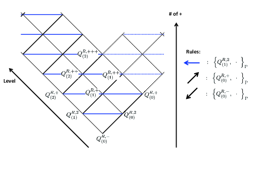
Figure 1: The tower structure of conserved charges.

Note that $\widetilde{Q}^{R,+}\,(=Q_{(2)}^{R,+})$ looks like an affine generator at a glance from the definition in analogy with the squashed S³ case KMY-QAA . However, it is not necessary to include $\widetilde{Q}^{R,+}$ into the defining relations so as to generate the whole tower of conserved charges. Eventually it is enough to take only $Q_{(1)}^{R,2}$ . In fact, $\widetilde{Q}^{R,+}\,(=Q^{R,+}_{(2)})$ is expressed in terms of lower conserved charges like

$$\Bigl{\{}Q^{R,2}_{(1)},Q^{R,+}_{(1)}\Bigr{\}}_{\rm P} = -\widetilde{Q}^{R,+}-\frac{\sqrt{C}}{2}\sinh\left(\frac{\sqrt{C}}{2}Q^{R,-}_{(0)}\right)\left(Q^{R,2}_{(1)}\right)^{2}$$

$$+\frac{\sqrt{C}}{4}\sinh\left(\frac{\sqrt{C}}{2}Q^{R,-}_{(0)}\right)Q^{R,2}_{(0)}Q^{R,2}_{(1)}\,.$$

and can be regarded as one of the level 2 conserved charges.

This is the reason that we have assigned the subscript $(2)$ as $\widetilde{Q}^{R,+}=Q_{(2)}^{R,+}$ . An interpretation why the structure of this kind happens will be explained from the viewpoint of Riemann spheres later.

There is another way to represent the tower of conserved charges. It is worth noting that the charges $\widetilde{Q}^{R,\pm}$ and $\widetilde{Q}^{R,2}$ also generate $q$-deformed Poincaré algebra. Hence, instead of $Q^{R,\pm}$ and $Q^{R,2}$ , one can use $\widetilde{Q}^{R,\pm}$ and $\widetilde{Q}^{R,2}$ as the level 0 charges. We refer to them as $\widetilde{Q}^{R,-}_{(0)}$ , $\widetilde{Q}^{R,2}_{(0)}$ , and $\widetilde{Q}^{R,+}_{(0)}$ . Then $Q^{R,2}$ plays a role of an affine generator in turn and should be called $\widetilde{Q}^{R,2}_{(1)}$ . The tower structure is depicted in Figure 2 .

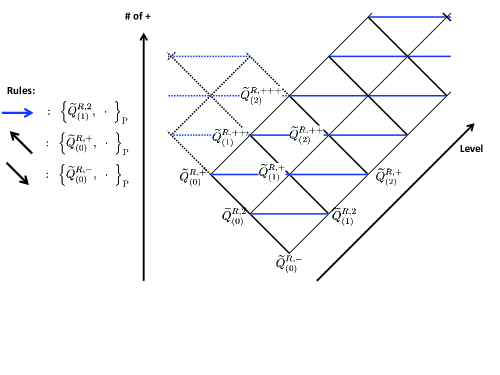
Figure 2: Another expression of the whole tower of conserved charges.

It would probably not be difficult to notice that there is a certain relation between the two representations. In fact, these are exchanged through the sign flip of $\sqrt{C}$ like

$$\sqrt{C}\quad\longleftrightarrow\quad-\sqrt{C}\,.$$ (38)

More concretely speaking, the flipping (38) exchanges the charges as

$$Q_{(n)}^{R,*}\quad\longleftrightarrow\quad\widetilde{Q}_{(n)}^{R,*}\qquad(*=\pm,2)\,.$$

Thus the one representation is dual to the other one through (38) .

Naively looking at the tower structure, one might think of that the two towers should be merged into a single V shape tower. However, it is not the case. To understand it accurately, it is of great value to note on the following Poisson brackets, as an example,

$$\left\{\widetilde{Q}^{R,2}_{(1)},\widetilde{Q}^{R,+}_{(0)}\right\}_{\rm P}=-\widetilde{Q}^{R,+}_{(1)}-\cosh\left(\frac{\sqrt{C}}{2}\widetilde{Q}^{R,-}_{(0)}\right)\widetilde{Q}^{R,+}_{(0)}\,,$$ (39)

$$\left\{Q^{R,2}_{(0)},Q^{R,+}_{(2)}\right\}_{\rm P}=-Q^{R,+}_{(1)}-\cosh\left(\frac{\sqrt{C}}{2}Q^{R,-}_{(0)}\right)Q^{R,+}_{(2)}\,.$$ (40)

The two equations are precisely identical but only the level assignment is different. The difference of the level assignment is very important because the interpretation of the right-hand sides of (39) and (40) depends on it.

The first relation (39) implies that $\widetilde{Q}^{R,+}_{(1)}$ is obtained when $\widetilde{Q}^{R,2}_{(1)}$ acts on $\widetilde{Q}^{R,+}_{(0)}$ . The right-hand side of (39) is interpreted that acting $\widetilde{Q}^{R,2}_{(1)}$ gives rise to the movement to right by one, because the lower conserved charges are discarded. This is depicted in Figure 2.

On the other hand, the second relation (40) says that acting $Q^{R,2}_{(0)}$ on $Q^{R,+}_{(2)}$ does not generate any new charge. At a glance, it seems that the right-hand side of (40) contains $Q^{R,+}_{(1)}$ sitting at the right of $Q^{R,+}_{(2)}$ and hence this operation also generates the movement to the right. However, $Q^{R,+}_{(1)}$ is lower than $Q^{R,+}_{(2)}$ in the level assignment in Figure 1. Thus $Q^{R,+}_{(2)}$ is picked up and after all $Q^{R,+}_{(2)}$ keeps staying under the action of $Q^{R,2}_{(0)}$ . In fact, any charges remain the same position under the action of $Q^{R,2}_{(0)}$ and the tower structure in Figure 1 is determined. This is the trick to determine the tower structure that is semi-infinite in a certain direction like Yangians rather than quantum affine algebras.

Finally we comment on the Yangian limit. When taking the $C\to 0$ limit, the $SL(2,\mathbb{R})_{\rm R}$ Yangian should be reproduced from the exotic symmetry discussed here. This limit is not obvious in the representations given in Figures 1 and 2. The level 0 charges in the $SL(2,\mathbb{R})_{\rm R}$ Yangian are obtained from the charges with $2,\pm$ . Then the level 1 charges are obtained from the charges with more $+$ . For example, the level 1 charge with $+$ is obtained from $Q_{(1)}^{R,++}$ in (35) by multiplying $1/\sqrt{C}$ before taking the $C\to 0$ limit. In fact, there is a better basis of the charges so that the Yangian limit is manifest. For this basis, it will be explained in future .

4.3 The right Lax pairs

It is a turn to consider Lax pairs in the right description. We refer to the Lax pairs as the right Lax pairs. Indeed, there are some ways to derive the right Lax pairs. Here we shall take a scaling limit of space-like or time-like warped AdS₃ spaces. Here we follow a different derivation from the one discussed in KY-Sch because the argument on the left-right duality becomes much clearer.

The metrics of space-like and time-like warped AdS₃ are given by, respectively warped ,

$$ds^{2}=\frac{L^{2}}{2}\left[{\rm Tr}\left(J^{2}\right)-2\widetilde{C}\left({\rm Tr}\left[T^{1}J\right]\right)^{2}\right]\qquad(\mbox{space-like})\,,$$ (41)

$$ds^{2}=\frac{L^{2}}{2}\left[{\rm Tr}\left(J^{2}\right)-2\widetilde{C}\left({\rm Tr}\left[T^{0}J\right]\right)^{2}\right]\qquad(\mbox{time-like})\,.$$ (42)

The constant parameter $\widetilde{C}$ is a deformation parameter. When $\widetilde{C}=0$, the metrics (41) and (42) degenerate to the one of AdS₃ with radius $L$ .

Let us start from a scaling limit of the space-like warped AdS₃ to the Schrödinger spacetime (The process is the same for the time-like). First, the metric (41) is rewritten in terms of $T^{\pm}$ as

$$ds^{2}=\frac{L^{2}}{2}\left[{\rm Tr}\left(J^{2}\right)-\widetilde{C}\left({\rm Tr}\left[T^{-}J\right]\right)^{2}+2\widetilde{C}{\rm Tr}\left[T^{-}J\right]{\rm Tr}\left[T^{+}J\right]-\widetilde{C}\left({\rm Tr}\left[T^{+}J\right]\right)^{2}\right]\,.$$

Then $T^{\pm}$ is rescaled like

$$T^{-}\to\sqrt{\frac{2C}{\widetilde{C}}}\,T^{-}\,,\qquad T^{+}\to\sqrt{\frac{\widetilde{C}}{2C}}\,T^{+}\,.$$ (43)

The resulting metric is given by

$$ds^{2}=\frac{L^{2}}{2}\left[{\rm Tr}\left(J^{2}\right)-2C\left({\rm Tr}\left[T^{-}J\right]\right)^{2}+2\widetilde{C}{\rm Tr}\left[T^{-}J\right]{\rm Tr}\left[T^{+}J\right]-\frac{\widetilde{C}^{2}}{2C}\left({\rm Tr}\left[T^{+}J\right]\right)^{2}\right]\,.$$

Finally, by taking the following limit

$$\widetilde{C}\to 0\qquad\mbox{with}~{}~{}C~{}~{}\mbox{fixed}\,,$$

the metric of the Schrödinger spacetime (7) is reproduced.

Our strategy here is to apply the same scaling limit to the Lax pairs in warped AdS₃ sigma models so as to obtain the right Lax pairs of the Schrödinger sigma models. The classical action of two-dimensional non-linear sigma models defined on space-like warped AdS₃ is given by

$$S = -\int^{\infty}_{-\infty}\!\!\!dt\int^{\infty}_{-\infty}\!\!\!dx\,\eta^{\mu\nu}\left[{\rm Tr}\left(J_{\mu}J_{\nu}\right)-2\widetilde{C}\,{\rm Tr}\left(T^{1}J_{\mu}\right){\rm Tr}\left(T^{1}J_{\nu}\right)\right]\,.$$ (44)

The right Lax pair is basically given in Cherednik ; FR and its expression is

$$L^{R}_{\pm}(x;\lambda_{R})=-\frac{\sinh\alpha}{\sinh\left(\alpha\pm\lambda_{R}\right)}\left[-T^{0}J^{0}_{\pm}+T^{2}J^{2}_{\pm}+\frac{\cosh\left(\alpha\pm\lambda_{R}\right)}{\cosh\alpha}T^{1}J^{1}_{\pm}\right]\,,$$ (45)

$$\hskip 85.35826ptJ_{\pm}=J_{t}\pm J_{x}\,,\qquad\sqrt{\widetilde{C}}=\tanh\alpha\,.$$

Then by using the isomorphism of the $sl(2)$ algebra KMY-monodromy

$$\left(T^{0}\pm T^{2}\right)\to{\rm e}^{\mp\lambda_{R}}\left(T^{0}\pm T^{2}\right)\,,$$ (46)

the Lax pair (45) is rewritten as

$$L^{R_{+}}_{\pm}(x;\lambda_{R_{+}}) = -\frac{\sinh\alpha}{\sinh\left(\alpha\pm\lambda_{R_{+}}\right)}\left[-\frac{1}{2}{\rm e}^{+\lambda_{R_{+}}}\left(T^{0}-T^{2}\right)\left(J^{0}_{\pm}+J^{2}_{\pm}\right)\right.$$ (47)

$$\left.-\frac{1}{2}{\rm e}^{-\lambda_{R_{+}}}\left(T^{0}+T^{2}\right)\left(J^{0}_{\pm}-J^{2}_{\pm}\right)+\frac{\cosh\left(\alpha\pm\lambda_{R_{+}}\right)}{\cosh\alpha}T^{1}J^{1}_{\pm}\right]\,,$$

where $\lambda_{R}$ has been renamed $\lambda_{R_{+}}$ because the fundamental domain of $\lambda_{R_{+}}$ is now just half of the one of $\lambda_{R}$ , namely the periodicity of $\lambda_{R_{+}}$ is $\pi$ while that of $\lambda_{R}$ is $2\pi$ . According to this division, the number of poles contained in the Lax pair is also reduced from four to two. Thus the isomorphism (46) leads to the decomposition of the Lax pair with four poles into a pair of the Lax pairs with two poles KMY-monodromy . The Lax pair (47) is one of the Lax pairs with two poles.

The other Lax pair with two poles can be obtained through the $sl(2)$ isomorphism

$$\left(T^{0}\pm T^{2}\right)\to{\rm e}^{\pm\lambda_{R}}\left(T^{0}\pm T^{2}\right)\,.$$ (48)

As a result, the Lax pair is given by

$$L^{R_{-}}_{\pm}(x;\lambda_{R_{-}}) = -\frac{\sinh\alpha}{\sinh\left(\alpha\pm\lambda_{R_{-}}\right)}\left[-\frac{1}{2}{\rm e}^{-\lambda_{R_{-}}}\left(T^{0}-T^{2}\right)\left(J^{0}_{\pm}+J^{2}_{\pm}\right)\right.$$

$$\left.-\frac{1}{2}{\rm e}^{+\lambda_{R_{-}}}\left(T^{0}+T^{2}\right)\left(J^{0}_{\pm}-J^{2}_{\pm}\right)+\frac{\cosh\left(\alpha\pm\lambda_{R_{-}}\right)}{\cosh\alpha}T^{1}J^{1}_{\pm}\right]\,,$$

where $\lambda_{R}$ has been renamed $\lambda_{R_{-}}$ on the same score.

The scaling limits for (47) and (4.3) give rise to the following right Lax pairs,

$$L^{R_{\pm}}_{\mu}(\lambda_{R_{\pm}})=\frac{1}{1-\lambda_{R_{\pm}}^{2}}\Bigl{[}-T^{+}\left(-J^{-}_{\mu}+\lambda_{R_{\pm}}\epsilon_{\mu\nu}J^{-,\nu}\right)\Bigr{.}$$ (50)

$$\qquad\qquad\quad\left.+T^{2}\left(-J^{2}_{\mu}+\lambda_{R_{\pm}}\epsilon_{\mu\nu}J^{2,\nu}\pm\sqrt{C}\lambda_{R_{\pm}}J^{-}_{\mu}\mp\sqrt{C}\lambda_{R_{\pm}}^{2}\epsilon_{\mu\nu}J^{-,\nu}\right)\right.$$

$$\qquad\qquad\quad\left.-T^{-}\Bigl{(}-J^{+}_{\mu}+\lambda_{R_{\pm}}\epsilon_{\mu\nu}J^{+,\nu}\pm\sqrt{C}\lambda_{R_{\pm}}J^{2}_{\mu}\mp\sqrt{C}\lambda_{R_{\pm}}^{2}\epsilon_{\mu\nu}J^{2,\nu}\right.$$

$$\qquad\qquad\qquad\qquad+C\lambda_{R_{\pm}}\epsilon_{\mu\nu}J^{-,\nu}-C\lambda_{R_{\pm}}^{2}J^{-}_{\mu}\Bigr{)}\Bigr{]}\,,$$

where we have rescaled $\lambda_{R_{\pm}}$ as $\lambda_{R_{\pm}}\to\alpha\lambda_{R_{\pm}}$ before taking the scaling limit. The Lax pairs (50) are also obtained by performing the following isomorphism

$$T^{-}\to T^{-}\,,$$

$$T^{2}\to T^{2}\mp\sqrt{C}\lambda_{R_{\pm}}T^{-}\,,$$ (51)

$$T^{+}\to T^{+}\mp\sqrt{C}\lambda_{R_{\pm}}T^{2}+\frac{C}{2}\lambda_{R_{\pm}}^{2}T^{-}\,,$$

to the right Lax pair in KY-Sch .

It is easy to check that the equations of motion (11) are reproduced from the commutation relations

$$\left[\partial_{t}-L^{R_{\pm}}_{t}(x;\lambda_{R_{\pm}}),\partial_{x}-L^{R_{\pm}}_{x}(\lambda_{R_{\pm}})\right]=0\,.$$ (52)

Then the monodromy matrices are given by

$$U^{R_{\pm}}(\lambda_{R_{\pm}})={\rm P}\exp\left[\int^{\infty}_{-\infty}\!\!\!dx~{}L^{R_{\pm}}_{x}(x;\lambda_{R_{\pm}})\right]\,.$$ (53)

These are conserved quantities and by expanding them with respect to $\lambda_{R_{\pm}}$ an infinite set of conserved charges are obtained. By following the procedure in Maillet  , the right $r$/$s$-matrices are given by

$$r^{R,_{\pm}}(\lambda_{R,_{\pm}},\mu_{R,_{\pm}}) = \left(h(\lambda_{R,_{\pm}})+h(\mu_{R,_{\pm}})\right)$$

$$\times\Biggl{[}\frac{1}{2\left(\lambda_{R,_{\pm}}-\mu_{R,_{\pm}}\right)}\left(-T^{+}\otimes T^{-}-T^{-}\otimes T^{+}+T^{2}\otimes T^{2}\right)$$

$$\hskip 28.45274pt\pm\frac{\sqrt{C}}{4}\left(T^{-}\otimes T^{2}-T^{2}\otimes T^{-}\right)\Biggr{]}\,,$$

$$s^{R,_{\pm}}(\lambda_{R,_{\pm}},\mu_{R,_{\pm}}) = \left(h(\lambda_{R,_{\pm}})-h(\mu_{R,_{\pm}})\right)$$

$$\times\Biggl{[}\frac{1}{2\left(\lambda_{R,_{\pm}}-\mu_{R,_{\pm}}\right)}\left(-T^{+}\otimes T^{-}-T^{-}\otimes T^{+}+T^{2}\otimes T^{2}\right)$$

$$\hskip 28.45274pt\pm\frac{\sqrt{C}}{4}\left(T^{-}\otimes T^{2}-T^{2}\otimes T^{-}\right)\Biggr{]}\,,$$

with $h(\lambda)$ defined in (22) . These satisfy the extended classical Yang-Baxter equation. The $r$-matrix cannot be rewritten into the skew symmetric form with respect to the difference of spectral parameters again.

Thus there are the two Lax pairs with two poles in the right description. Recall that there are two Lax pairs with two poles also in the left description. In fact, there is a relation between the right and left descriptions as we will see in the next subsection.

4.4 The gauge equivalence and Riemann sphere

So far, we have seen that there are the two descriptions 1) the left description and 2) the right description. Let us show that the two descriptions are related through a gauge transformation and eventually equivalent.

Before arguing the gauge transformation, it is necessary to fix the relations between the spectral parameters in the two descriptions. These are obtained by taking a scaling limit of the spectral parameter relations, for example, in the case of space-like warped AdS₃ sigma models,

$$\lambda_{L_{\pm}}=\frac{\tanh\alpha}{\tanh\lambda_{R_{\pm}}}\quad\qquad\mbox{(warped~{}AdS${}_{3}$)}\,.$$

The resulting relations after the scaling limit are simply given by

$$\lambda_{L_{\pm}}=\frac{1}{\lambda_{R_{\pm}}}\qquad\quad\mbox{(Schr\"{o}dinger)}\,.$$ (54)

This is the same as in the case of principal chiral models, up to the subscript $\pm$ .

Now it is a turn to show the gauge equivalence. With the relations in (54) , the right Lax pairs are rewritten as

$$L^{R_{\pm}}_{\mu}(\lambda_{R_{\pm}}) = -\frac{1}{1-\lambda_{L_{\pm}}^{2}}\Bigl{[}-T^{+}\left(-\lambda_{L_{\pm}}^{2}J^{-}_{\mu}+\lambda_{L_{\pm}}\epsilon_{\mu\nu}J^{-,\nu}\right)\Bigr{.}$$

$$\hskip 56.9055pt\left.+T^{2}\left(-\lambda_{L_{\pm}}^{2}J^{2}_{\mu}+\lambda_{L_{\pm}}\epsilon_{\mu\nu}J^{2,\nu}\pm\sqrt{C}\lambda_{L_{\pm}}J^{-}_{\mu}\mp\sqrt{C}\epsilon_{\mu\nu}J^{-,\nu}\right)\right.$$

$$\hskip 56.9055pt\Bigl{.}-T^{-}\Bigl{(}-\lambda_{L_{\pm}}^{2}J^{+}_{\mu}+\lambda_{L_{\pm}}\epsilon_{\mu\nu}J^{+,\nu}\pm\sqrt{C}\lambda_{L_{\pm}}J^{2}_{\mu}\mp\sqrt{C}\epsilon_{\mu\nu}J^{2,\nu}$$

$$\hskip 71.13188pt+C\lambda_{L_{\pm}}\epsilon_{\mu\nu}J^{-,\nu}-CJ^{-}_{\mu}\Bigr{)}\Bigr{]}\,.$$

Then let us perform the gauge transformation like

$$\Bigl{[}L^{R_{\pm}}_{\mu}(\lambda_{R_{\pm}})\Bigr{]}^{g}\equiv\partial_{\mu}g\cdot g^{-1}+gL^{R_{\pm}}_{\mu}(\lambda_{R_{\pm}})g^{-1}$$

$$= \frac{1}{1-\lambda_{L_{\pm}}^{2}}g\Bigl{\{}-T^{+}\left[J^{-}_{\mu}-\lambda_{L_{\pm}}\epsilon_{\mu\nu}J^{-,\nu}\right]\Bigr{.}$$

$$\quad\left.+T^{2}\left[\left(J^{2}_{\mu}\pm\sqrt{C}\epsilon_{\mu\nu}J^{-,\nu}\right)-\lambda_{L_{\pm}}\epsilon_{\mu\nu}\left(J^{2,\nu}\pm\sqrt{C}\epsilon^{\nu\rho}J^{-}_{\rho}\right)\right]\right.$$

$$\quad\Bigl{.}-T^{-}\Bigl{[}\left(J^{+}_{\mu}\pm\sqrt{C}\epsilon_{\mu\nu}J^{2,\nu}+CJ^{-}_{\mu}\right)-\lambda_{L_{\pm}}\epsilon_{\mu\nu}\left(J^{+,\nu}\pm\sqrt{C}\epsilon^{\nu\rho}J^{2}_{\rho}+CJ^{-,\nu}\right)\Bigr{]}\Bigr{\}}g^{-1}$$

$$= L^{L_{\pm}}_{\mu}(\lambda_{L_{\pm}})\,.$$

Thus the Lax pairs in the left and right descriptions are gauge-equivalent,

$$\Bigl{[}L^{R_{\pm}}_{\mu}(\lambda_{R_{\pm}})\Bigr{]}^{g}=L^{L_{\pm}}_{\mu}(\lambda_{L_{\pm}})\,.$$ (55)

At the level of monodromy matrix, (55) is recast into

$$U^{R_{\pm}}(\lambda_{\pm})=g_{\infty}^{-1}\cdot U^{L_{\pm}}(\lambda_{\pm})\cdot g_{\infty}\,.$$ (56)

Thus the right description is gauge-equivalent globally to the left one.

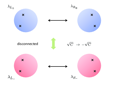
Figure 3: The spaces of spectral parameters are described as Riemann spheres with two punctures. The blue spheres are gauge-equivalent to the red ones.

We comment on the Riemann sphere picture of this equivalence as depicted in Figure 3. The pole structure of the Lax pairs is figured out from the expressions. For each of them, the space of spectral parameter is represented by a Riemann sphere with two punctures. The spectral parameter relations (54) lead to the equivalence of the Riemann spheres of $\lambda_{R_{+}}$ and $\lambda_{L_{+}}$ Similar equivalence holds for $\lambda_{R_{-}}$ and $\lambda_{L_{-}}$ .

Now that we have two independent Riemann spheres with two punctures for the subscripts $+$ and $-$ . Note that the two spheres are related one another through the sign flipping of $\sqrt{C}$ . Then the one representation of the exotic symmetry comes from the Riemann sphere for $+$ and the other one comes from that for $-$ .

However, this sign flipping is equivalent to the following $sl(2)$ isomorphism and the field redefinition,

$$T^{\pm}~{}~{}\to~{}~{}-T^{\pm}\,,\qquad J^{\pm}~{}~{}\to~{}~{}-J^{\pm}\,.$$ (57)

This means that the sign flipping of $\sqrt{C}$ is written as a gauge transformation. Thus the two Riemann spheres with $+$ and $-$ are also gauge-equivalent. For this reason, one of the candidate of affine generators is realized as one of the second level conserved charges. That is, the level 0 charges with $+$ and $2$ on the one side are realized as level 2 charges on the other side through the gauge transformation. Thus the two representations of the exotic symmetry are also gauge-equivalent. In other words, the level assignment is nothing but a gauge degree of freedom.

The resulting geometry in Figure 3 can also be interpreted as a scaling limit of the Riemann spheres in the case of warped AdS₃ sigma models (See KMY-monodromy ). Because the scaling limit contains the $\widetilde{C}\to 0$ limit, the cut shrinks to a point. After that, the geometry is given by Figure 3.

Finally we shall summarize the conserved charges of infinite-dimensional symmetries and the expansion points of the monodromy matrices in Table 1. It is easy to understand the expansion points for the $sl(2,{\mathbb{R}})_{\rm L}$ Yangian with the relations between the spectral parameters (54). The conserved charges for the affine $q$-deformed Poincaré algebra can also be obtained by expanding the right monodromy matrices $U^{R_{\pm}}(\lambda_{R_{\pm}})$ around $\lambda_{R_{\pm}}=\infty$ future . According to this, the left expansion point is automatically determined through (54) . Actually, there is a slight difference between the charges obtained in the subsection 4.2 and the ones obtained from the monodromy matrices. The two sets of the charges are homomorphic but not always isomorphic depending on the sign of $C$ . The details will be reported in future .

Charges $\setminus$ Monodromies	$\qquad U^{L_{\pm}}(\lambda_{L_{\pm}})\qquad$	$\quad U^{R_{\pm}}(\lambda_{R_{\pm}})\quad$
$SL(2,{\mathbb{R}})_{\rm L}$ Yangian	$\infty$	0
exotic symmetry	0	$\infty$
local charges	$\pm 1$	$\pm 1$

Table 1: The charges and the expansion points of monodromy matrices.

5 Conclusion and Discussion

We have unveiled an exotic hidden symmetry in Schrödinger sigma models. This is an infinite-dimensional extension of $q$-deformed Poincaré algebra. We have argued the tower structure of the conserved charges by directly evaluating the Serre relations. The tower is generated in an exotic way and it looks like a tilted Yangian algebra. There are two representations of the tower structure for the exotic symmetry, depending on the choice of the level 0 charges, and the one is mapped to the other simply through the sign flipping of $\sqrt{C}$ .

There are the two descriptions to describe the classical dynamics: 1) the left description based on $SL(2,\mathbb{R})_{\rm L}$ and 2) the right description based on $U(1)_{\rm R}$ . Then the monodromy matrices in the two descriptions have been shown to be gauge-equivalent via the relation between the spectral parameters. Moreover, we have given a simple Riemann sphere interpretation of this equivalence. It can be understood both as the remnant of the left-right duality of $SL(2,{\mathbb{R}})$ principal chiral models and as a decoupling limit of the hybrid integrable structure of warped AdS₃ sigma models.

One may suspect that there might be an isomorphism between the algebra for the exotic symmetry and the standard Yangian. However, at a glance, the resulting algebra looks different from the Yangian because it contains a $q$-deformed Poincaré algebra, which has a constant parameter, as the level 0 part. Nevertheless, there might be such an isomorphism because the gauge-equivalence of the monodromy matrices means that both the exotic symmetry and the Yangian are realized by expanding a single monodromy matrix.

At least so far, we are not sure for the mathematical formulation of the exotic symmetry itself. It is important to reveal the Hopf algebraic structure of this symmetry, especially the coproduct. We believe that there should be a well-defined mathematical structure for it, not depending on the sigma model action, like in the case of non-local charges in $O(N)$ non-linear sigma models Luscher1 ; Luscher2 and Yangian Drinfeld .

It is nice to look for some applications of the exotic symmetry in the context of warped AdS₃/dipole CFT₂ Guica ; SS . This duality is proposed as a toy model of the Kerr/CFT correspondence Kerr/CFT . It would also be interesting to consider the quantum integrability of Schrödinger sigma models, though we have confined ourselves to the classical integrability so far. In this direction it is worth trying to construct the Bethe ansatz by following the procedure in PW ; quantum1 ; quantum2 ; quantum3 .

We hope that the exotic symmetry unveiled here would play a significant role in exploring a new aspect of integrable deformations of AdS/CFT.

Acknowledgments

We would like to thank N. Dorey, N. MacKay, M. Magro, V. Regelskis and B. Vicedo for useful discussions, and especially T. Matsumoto for a collaboration at an early stage and reading the manuscript carefully. The work of IK was supported by the Japan Society for the Promotion of Science (JSPS). The work of KY was supported by the scientific grants from the Ministry of Education, Culture, Sports, Science and Technology (MEXT) of Japan (No. 22740160). This work was also supported in part by the Grant-in-Aid for the Global COE Program “The Next Generation of Physics, Spun from Universality and Emergence” from MEXT, Japan.

Appendix

Appendix A The current algebra for $j^{R}_{\mu}$ and $\widetilde{j}^{R}_{\mu}$

We show the Poisson brackets of the conserved currents $j^{R}_{\mu}$ and $\widetilde{j}^{R}_{\mu}$ that are used to compute the algebra of conserved charges in section 4.

The Poisson brackets between $j^{R}_{\mu}$ are evaluated as

$$\Bigl{\{}j^{R,-}_{t}(x),j^{R,-}_{t}(y)\Bigr{\}}_{\rm P} = 0\,,$$

$$\Bigl{\{}j^{R,-}_{t}(x),j^{R,2}_{t}(y)\Bigr{\}}_{\rm P} = {\rm e}^{\sqrt{C}\chi}j^{R,-}_{t}(x)\delta(x-y)\,,$$

$$\Bigl{\{}j^{R,-}_{t}(x),j^{R,+}_{t}(y)\Bigr{\}}_{\rm P} = j^{R,2}_{t}(x)\delta(x-y)\,,$$

$$\Bigl{\{}j^{R,2}_{t}(x),j^{R,2}_{t}(y)\Bigr{\}}_{\rm P} = -\frac{\sqrt{C}}{2}\epsilon(x-y)\left[j^{R,2}_{t}(x){\rm e}^{\sqrt{C}\chi}j^{R,-}_{t}(y)+{\rm e}^{\sqrt{C}\chi}j^{R,-}_{t}(x)j^{R,2}_{t}(y)\right]\,,$$

$$\Bigl{\{}j^{R,2}_{t}(x),j^{R,+}_{t}(y)\Bigr{\}}_{\rm P} = {\rm e}^{\sqrt{C}\chi}j^{R,+}_{t}(x)\delta(x-y)$$

$$-\frac{\sqrt{C}}{2}\epsilon(x-y)\left[j^{R,2}_{t}(x)j^{R,2}_{t}(y)+{\rm e}^{\sqrt{C}\chi}j^{R,-}_{t}(x)j^{R,+}_{t}(y)\right]\,,$$

$$\Bigl{\{}j^{R,+}_{t}(x),j^{R,+}_{t}(y)\Bigr{\}}_{\rm P} = -\frac{\sqrt{C}}{2}\epsilon(x-y)\left[j^{R,+}_{t}(x)j^{R,2}_{t}(y)+j^{R,2}_{t}(x)j^{R,+}_{t}(y)\right]\,,$$

$$\Bigl{\{}j^{R,-}_{t}(x),j^{R,-}_{x}(y)\Bigr{\}}_{\rm P} = 0\,,$$

$$\Bigl{\{}j^{R,-}_{t}(x),j^{R,2}_{x}(y)\Bigr{\}}_{\rm P} = {\rm e}^{\sqrt{C}\chi}j^{R,-}_{x}(x)\delta(x-y)\,,$$

$$\Bigl{\{}j^{R,-}_{t}(x),j^{R,+}_{x}(y)\Bigr{\}}_{\rm P} = j^{R,2}_{x}(x)\delta(x-y)+\sqrt{C}{\rm e}^{\sqrt{C}\chi}j^{R,-}_{t}(x)\delta(x-y)$$

$$-{\rm e}^{\sqrt{C}\chi(x)}\partial_{x}\delta(x-y)\,,$$

$$\Bigl{\{}j^{R,2}_{t}(x),j^{R,-}_{x}(y)\Bigr{\}}_{\rm P} = -{\rm e}^{\sqrt{C}\chi}j^{R,-}_{x}(x)\delta(x-y)\,,$$ (58)

$$\Bigl{\{}j^{R,2}_{t}(x),j^{R,2}_{x}(y)\Bigr{\}}_{\rm P} = -2\sqrt{C}{\rm e}^{2\sqrt{C}\chi}j^{R,-}_{t}(x)\delta(x-y)+{\rm e}^{2\sqrt{C}\chi(x)}\partial_{x}\delta(x-y)$$

$$-\frac{\sqrt{C}}{2}\epsilon(x-y)\left[j^{R,2}_{t}(x){\rm e}^{\sqrt{C}\chi}j^{R,-}_{x}(y)+{\rm e}^{\sqrt{C}\chi}j^{R,-}_{t}(x)j^{R,2}_{x}(y)\right]\,,$$

$$\Bigl{\{}j^{R,2}_{t}(x),j^{R,+}_{x}(y)\Bigr{\}}_{\rm P} = {\rm e}^{\sqrt{C}\chi}j^{R,+}_{x}(x)\delta(x-y)$$

$$-\frac{\sqrt{C}}{2}\epsilon(x-y)\left[j^{R,2}_{t}(x)j^{R,2}_{x}(y)+{\rm e}^{\sqrt{C}\chi}j^{R,-}_{t}(x)j^{R,+}_{x}(y)\right]\,,$$

$$\Bigl{\{}j^{R,+}_{t}(x),j^{R,-}_{x}(y)\Bigr{\}}_{\rm P} = -j^{R,2}_{x}(x)\delta(x-y)+\sqrt{C}{\rm e}^{\sqrt{C}\chi}j^{R,-}_{t}(x)\delta(x-y)$$

$$-{\rm e}^{\sqrt{C}\chi(x)}\partial_{x}\delta(x-y)\,,$$

$$\Bigl{\{}j^{R,+}_{t}(x),j^{R,2}_{x}(y)\Bigr{\}}_{\rm P} = -{\rm e}^{\sqrt{C}\chi}j^{R,+}_{x}(x)\delta(x-y)$$

$$-\frac{\sqrt{C}}{2}\epsilon(x-y)\left[j^{R,+}_{t}(x){\rm e}^{\sqrt{C}\chi}j^{R,-}_{x}(y)+j^{R,2}_{t}(x)j^{R,2}_{x}(y)\right]\,,$$

$$\Bigl{\{}j^{R,+}_{t}(x),j^{R,+}_{x}(y)\Bigr{\}}_{\rm P} = -\frac{\sqrt{C}}{2}\epsilon(x-y)\left[j^{R,+}_{t}(x)j^{R,2}_{x}(y)+j^{R,2}_{t}(x)j^{R,+}_{x}(y)\right]\,,$$

$$\Bigl{\{}j^{R,-}_{x}(x),j^{R,-}_{x}(y)\Bigr{\}}_{\rm P} = 0\,,$$

$$\Bigl{\{}j^{R,-}_{x}(x),j^{R,2}_{x}(y)\Bigr{\}}_{\rm P} = 0\,,$$

$$\Bigl{\{}j^{R,-}_{x}(x),j^{R,+}_{x}(y)\Bigr{\}}_{\rm P} = \sqrt{C}{\rm e}^{\sqrt{C}\chi}j^{R,-}_{x}(x)\delta(x-y)\,,$$

$$\Bigl{\{}j^{R,2}_{x}(x),j^{R,2}_{x}(y)\Bigr{\}}_{\rm P} = -\frac{\sqrt{C}}{2}\epsilon(x-y)\left[j^{R,2}_{x}(x){\rm e}^{\sqrt{C}\chi}j^{R,-}_{x}(y)+{\rm e}^{\sqrt{C}\chi}j^{R,-}_{x}(x)j^{R,2}_{x}(y)\right]\,,$$

$$\Bigl{\{}j^{R,2}_{x}(x),j^{R,+}_{x}(y)\Bigr{\}}_{\rm P} = -\frac{\sqrt{C}}{2}\epsilon(x-y)\left[j^{R,2}_{x}(x)j^{R,2}_{t}(y)+{\rm e}^{\sqrt{C}\chi}j^{R,-}_{x}(x)j^{R,+}_{t}(y)\right]\,,$$

$$\Bigl{\{}j^{R,+}_{x}(x),j^{R,+}_{x}(y)\Bigr{\}}_{\rm P} = -\frac{\sqrt{C}}{2}\epsilon(x-y)\left[j^{R,+}_{x}(x)j^{R,2}_{x}(y)+j^{R,2}_{x}(x)j^{R,+}_{x}(y)\right]\,.$$

Note that non-ultra local terms are contained only in the Poisson brackets between $j^{R,a}_{t}$ and $j^{R,b}_{x}$ . This is the same as in the case of principal chiral models. Thus there is no subtlety concerned with non-ultra local terms in computing (non-affine) $q$-deformed Poincaré algebra. The algebra for $\widetilde{j}^{R}_{\mu}$ can be obtained by flipping the sign of $\sqrt{C}$ and hence the property is the same as the above algebra.

Finally let us show the Poisson brackets between $j^{R}_{\mu}(x)$ , $\widetilde{j}^{R}_{\mu}(x)$ and $J_{\mu}(x)$ . Because the complete list of the brackets is quite messy, we present the Poisson brackets used to discuss the exotic symmetry in section 4. The Poisson brackets used in this paper are the following:

$$\Bigl{\{}j^{R,2}_{t}(x),\widetilde{j}^{R,2}_{t}(y)\Bigr{\}}_{\rm P} = -\frac{1}{2}\partial_{x}\left(\epsilon(x-y){\rm e}^{\sqrt{C}\chi(x)}\right)\widetilde{j}^{R,2}_{t}(y)$$

$$-\frac{1}{2}j^{R,2}_{t}(x)\partial_{y}\left(\epsilon(x-y){\rm e}^{-\sqrt{C}\chi(y)}\right)\,,$$

$$\Bigl{\{}j^{R,+}_{t}(x),\widetilde{j}^{R,2}_{t}(y)\Bigr{\}}_{\rm P} = \frac{\sqrt{C}}{2}\epsilon(x-y)j^{R,2}_{t}(x)\widetilde{j}^{R,2}_{t}(y)+2J^{+}_{t}(x)\delta(x-y)$$

$$-\frac{1}{2}j^{R,+}_{t}(x)\partial_{y}\left(\epsilon(x-y){\rm e}^{-\sqrt{C}\chi(y)}\right)+2\sqrt{C}\partial_{x}\delta(x-y)\,,$$

$$\Bigl{\{}j^{R,+}_{t}(x),J^{+}_{t}(y)\Bigr{\}}_{\rm P} = -\frac{\sqrt{C}}{2}\epsilon(x-y)j^{R,+}_{t}(x)J^{2}_{t}(y)-\sqrt{C}j^{R,+}_{x}(x)\delta(x-y)\,.$$

$$\Bigl{\{}\widetilde{j}^{R,2}_{t}(x),J^{+}_{t}(y)\Bigr{\}}_{\rm P} = \frac{\sqrt{C}}{2}\epsilon(x-y)\widetilde{j}^{R,2}_{t}(x)J^{2}_{t}(y)-\widetilde{j}^{R,+}_{t}(x)\delta(x-y)$$

$$-\sqrt{C}\partial_{x}\left({\rm e}^{-\sqrt{C}\chi(x)}\delta(x-y)\right)\,.$$

It is necessary for further computation to use the other brackets, as a matter of course.

Appendix B Prescriptions to treat non-ultra local terms

The current algebra presented in appendix A contains non-ultra local terms. They lead to some ambiguities in evaluating the Poisson brackets of conserved charges. We here explain how to treat the ambiguities.

The ambiguities come from the order of limits and depend on the species of charges contained in the Poisson bracket. To make this point clear, let us introduce the cut-offs to the integrations in the level 0 charges $Q_{(0)}^{R}$’s and the level 1 charges $Q_{(1)}^{R}$’s as follows:

$$Q^{R,+}_{(0)}(X_{1},X_{2}) \equiv \int^{X_{1}}_{-X_{2}}\!\!dx~{}j^{R,+}_{t}(x)\,,$$

$$Q^{R,2}_{(1)}(X_{1},X_{2}) \equiv \int^{X_{1}}_{-X_{2}}\!\!dx~{}\widetilde{j}^{R,2}_{t}(x)\,,$$

$$Q_{(1)}^{R,+}(X_{1},X_{2}) \equiv \frac{\sqrt{C}}{2}\int^{X_{1}}_{-X_{2}}\!\!dx\!\int^{X_{1}^{\prime}}_{-X_{2}^{\prime}}\!\!dx^{\prime}~{}\epsilon(x-x^{\prime})\,j^{R,2}_{t}(x)\widetilde{j}^{R,2}_{t}(x^{\prime})+2\int^{X_{1}^{\prime\prime}}_{-X_{2}^{\prime\prime}}\!\!\!dx^{\prime\prime}~{}J^{+}_{t}(x^{\prime\prime})\,,$$

$$Q^{R,++}_{(1)}(X_{1},X_{2}) \equiv -\frac{C}{4}\int^{X_{1}}_{-X_{2}}\!\!dx\!\int^{X_{1}^{\prime}}_{-X_{2}^{\prime}}\!\!dx^{\prime}\!\int^{X_{1}^{\prime\prime}}_{-X_{2}^{\prime\prime}}\!\!dx^{\prime\prime}~{}\epsilon(x-x^{\prime})\epsilon(x-x^{\prime\prime})j^{R,2}_{t}(x)j^{R,2}_{t}(x^{\prime})\widetilde{j}^{R,2}_{t}(x^{\prime\prime})$$

$$+\sqrt{C}\int^{X_{1}^{\prime\prime\prime}}_{-X_{2}^{\prime\prime\prime}}\!\!dx^{\prime\prime\prime}\!\int^{X_{1}^{\prime\prime\prime\prime}}_{-X_{2}^{\prime\prime\prime\prime}}\!\!dx^{\prime\prime\prime\prime}~{}\epsilon(x^{\prime\prime\prime}-x^{\prime\prime\prime\prime})j^{R,2}_{t}(x^{\prime\prime\prime})J^{+}_{t}(x^{\prime\prime\prime\prime})$$

$$-2\sqrt{C}\int^{X_{1}^{\prime\prime\prime\prime\prime}}_{-X_{2}^{\prime\prime\prime\prime\prime}}\!\!dx^{\prime\prime\prime\prime\prime}~{}j^{R,+}_{x}(x^{\prime\prime\prime\prime\prime})\,.$$

There is no ambiguity in the Poisson brackets between $Q_{(0)}^{R}$’s. Hence the first thing we consider is the bracket between $Q_{(0)}^{R}$ and $Q_{(1)}^{R}$ .

Let us, for example, see the following bracket,

$$\Bigl{\{}Q^{R,+}_{(0)}(X_{1},X_{2}),Q^{R,2}_{(1)}(Y_{1},Y_{2})\Bigr{\}}_{\rm P}$$

$$= 2\sqrt{C}\int^{X_{1}}_{-X_{2}}\!\!dx\!\int^{Y_{1}}_{-Y_{2}}\!\!dy~{}\partial_{x}\delta(x-y)+\mbox{(no~{}ambiguity)}$$

$$= 2\sqrt{C}\left[\theta(Y_{1}-X_{1})-\theta(Y_{2}-X_{2})\right]+\mbox{(no~{}ambiguity)}\,.$$

The value of the last expression depends on the order of limits. A possible resolution of this ambiguity is to follow the prescription proposed by MacKay MacKay ,

$$X_{1}=X_{2}\equiv X\,,\qquad Y_{1}=Y_{2}\equiv Y\,.$$ (60)

That is, $Q^{R,+}_{(0)}$ and $Q^{R,2}_{(1)}$ are regularized as

$$Q^{R,+}_{(0)}(X)\equiv\int^{X}_{-X}\!\!dx~{}j^{R,+}_{t}(x)\,,\qquad Q^{R,2}_{(1)}(Y)\equiv\int^{Y}_{-Y}\!\!dx~{}\widetilde{j}^{R,2}_{t}(x)\,.$$

The prescription (60) is used also in computing the Yangian algebra. Similarly, the other charges should be regularized following (60). For example, $Q^{R,+}_{(1)}$ is done as

$$Q_{(1)}^{R,+}(X) \equiv \frac{\sqrt{C}}{2}\int^{X}_{-X}\!\!dx\!\int^{X^{\prime}}_{-X^{\prime}}\!\!dx^{\prime}~{}\epsilon(x-x^{\prime})\,j^{R,2}_{t}(x)\widetilde{j}^{R,2}_{t}(x^{\prime})+2\int^{X^{\prime\prime}}_{-X^{\prime\prime}}\!\!\!dx^{\prime\prime}~{}J^{+}_{t}(x^{\prime\prime})\,.$$

Next let us evaluate the Poisson bracket between $Q^{R,+}_{(0)}(X)$ and $Q^{R,+}_{(1)}(Y)$ . In fact, there is another type of ambiguity. It is helpful to use the following integral formula,

$$\int^{b}_{-b}\!\!dx~{}\epsilon(x-c)\left[\delta(x-a)-\delta(x+a)\right]\qquad(a>0,~{}b>0)$$ (63)

$$= \int^{b}_{c}\!\!dx~{}\left[\delta(x-a)-\delta(x+a)\right]-\int^{c}_{-b}\!\!dx~{}\left[\delta(x-a)-\delta(x+a)\right]$$

$$= \left[\theta(b-a)-\theta(c-a)-\theta(-c-a)\right]-\left[\theta(c-a)-\theta(c+a)+\theta(a-b)\right]$$

$$= \left\{\begin{array}[]{cc}-2\theta(c-a)+2\theta(c+a)-2\theta(a-b)&\quad(-b<c<b)\\ 0&{\rm otherwise}\\ \end{array}\right.$$

$$= \left[\theta(c+b)-\theta(c-b)\right]\left[-2\theta(c-a)+2\theta(c+a)-2\theta(a-b)\right]\,,$$ (64)

where $c$ is a real constant. With (64), the bracket is evaluated as follows:

$$\Bigl{\{}Q^{R,+}_{(0)}(X),Q^{R,+}_{(1)}(Y)\Bigr{\}}_{\rm P}$$

$$= \frac{\sqrt{C}}{2}\int^{X}_{-X}\!\!dx\!\int^{Y}_{-Y}\!\!dy\!\int^{Y^{\prime}}_{-Y^{\prime}}\!\!dy^{\prime}~{}\epsilon(y-y^{\prime})j^{R,2}_{t}(y)\left(2\sqrt{C}\partial_{x}\delta(x-y^{\prime})\right)+\mbox{(no~{}ambiguity)}$$

$$= C\int^{Y}_{-Y}\!\!dy~{}j^{R,2}_{t}(y)\int^{Y^{\prime}}_{-Y^{\prime}}\!\!dy^{\prime}~{}\epsilon(y-y^{\prime})\left[\delta(y^{\prime}-X)-\delta(y^{\prime}+X)\right]+\mbox{(no~{}ambiguity)}$$

$$= 2C\int^{Y}_{-Y}dy~{}j^{R,2}_{t}(y)\left[\theta(y+Y^{\prime})-\theta(y-Y^{\prime})\right]$$

$$\hskip 56.9055pt\times\left[\theta(y-X)-\theta(y+X)+\theta(X-Y^{\prime})\right]+\mbox{(no~{}ambiguity)}$$

$$= 2C\int^{\min\{Y,Y^{\prime}\}}_{-\min\{Y,Y^{\prime}\}}dy~{}j^{R,2}_{t}(y)\left[\theta(y-X)-\theta(y+X)+\theta(X-Y^{\prime})\right]$$

$$\hskip 28.45274pt+\mbox{(no~{}ambiguity)}$$

$$= 2C\theta(X-Y^{\prime})\int^{\min\{Y,Y^{\prime}\}}_{-\min\{Y,Y^{\prime}\}}dy~{}j^{R,2}_{t}(y)-2C\int^{\min\{X,Y,Y^{\prime}\}}_{-\min\{X,Y,Y^{\prime}\}}dy~{}j^{R,2}_{t}(y)$$

$$\hskip 28.45274pt+\mbox{(no~{}ambiguity)}\,.$$

Thus the ambiguity of order of limits arises from the non-ultra local term. A possible resolution is to take the order of limits to maintain the defining relations in the mathematical formultation of the algebra. Indeed, the coproduct structure plays an important role in the case of Yangian MacKay . However, in the present case, the mathematical formulation of the exotic symmetry has not been clarified yet, and the coproduct is not fixed. Hence there is no criterion so far.

Here we have naively taken the $X\to\infty$ limit before the $Y^{\prime}\to\infty$ limit where the ambiguous term vanishes, simply because the order of limits which leads to a simpler result works well in the case of Yangian. If the coproduct prefers the other order of limits actually, we have to take the additional term into account.

It is a turn to evaluate the Poisson bracket between $Q^{R,+}_{(0)}$ and $Q^{R,++}_{(1)}$ . Note that $Q^{R,++}_{(1)}$ is regularized as

$$Q^{R,++}_{(1)}(X) \equiv -\frac{C}{4}\int^{X}_{-X}\!\!dx\!\int^{X^{\prime}}_{-X^{\prime}}\!\!dx^{\prime}\!\int^{X^{\prime\prime}}_{-X^{\prime\prime}}\!\!dx^{\prime\prime}~{}\epsilon(x-x^{\prime})\epsilon(x-x^{\prime\prime})j^{R,2}_{t}(x)j^{R,2}_{t}(x^{\prime})\widetilde{j}^{R,2}_{t}(x^{\prime\prime})$$

$$+\sqrt{C}\int^{X^{\prime\prime\prime}}_{-X^{\prime\prime\prime}}\!\!dx^{\prime\prime\prime}\!\int^{X^{\prime\prime\prime\prime}}_{-X^{\prime\prime\prime\prime}}\!\!dx^{\prime\prime\prime\prime}~{}\epsilon(x^{\prime\prime\prime}-x^{\prime\prime\prime\prime})j^{R,2}_{t}(x^{\prime\prime\prime})J^{+}_{t}(x^{\prime\prime\prime\prime})$$

$$-2\sqrt{C}\int^{X^{\prime\prime\prime\prime\prime}}_{-X^{\prime\prime\prime\prime\prime}}\!\!dx^{\prime\prime\prime\prime\prime}~{}j^{R,+}_{x}(x^{\prime\prime\prime\prime\prime})\,.$$

Then, by using the formula (64) , the bracket is rewritten as

$$\Bigl{\{}Q^{R,+}_{(0)}(X),Q^{R,++}_{(1)}(Y)\Bigr{\}}_{\rm P}$$

$$= \frac{C}{4}\int^{X}_{-X}\!\!dx\!\int^{Y}_{-Y}\!\!dy\!\int^{Y^{\prime}}_{-Y^{\prime}}\!\!dy^{\prime}\!\int^{Y^{\prime\prime}}_{-Y^{\prime\prime}}\!\!dy^{\prime\prime}~{}\epsilon(y-y^{\prime})\epsilon(y-y^{\prime\prime})j^{R,2}_{t}(y)j^{R,2}_{t}(y^{\prime})$$

$$\hskip 113.81102pt\times\left(2\sqrt{C}\partial_{x}\delta(x-y^{\prime\prime})\right)+\mbox{(no~{}ambiguity)}$$

$$= \frac{C\sqrt{C}}{2}\int^{Y}_{-Y}\!\!dy\!\int^{Y^{\prime}}_{-Y^{\prime}}\!\!dy^{\prime}~{}\epsilon(y-y^{\prime})j^{R,2}_{t}(y)j^{R,2}_{t}(y^{\prime})$$

$$\hskip 56.9055pt\times\int^{Y^{\prime\prime}}_{-Y^{\prime\prime}}\!\!dy^{\prime\prime}~{}\epsilon(y-y^{\prime\prime})\left[\delta(y^{\prime\prime}-X)-\delta(y^{\prime\prime}+X)\right]+\mbox{(no~{}ambiguity)}$$

$$= C\sqrt{C}\int^{Y}_{-Y}dy\!\int^{Y^{\prime}}_{-Y^{\prime}}\!\!dy^{\prime}~{}\epsilon(y-y^{\prime})j^{R,2}_{t}(y)j^{R,2}_{t}(y^{\prime})\left[\theta(y+Y^{\prime\prime})-\theta(y-Y^{\prime\prime}\right])$$

$$\hskip 56.9055pt\times\left[\theta(y-X)-\theta(y+X)+\theta(X-Y^{\prime\prime})\right]+\mbox{(no~{}ambiguity)}$$

$$= C\sqrt{C}\int^{\min\{Y,Y^{\prime\prime}\}}_{-\min\{Y,Y^{\prime\prime}\}}dy\!\int^{Y^{\prime}}_{-Y^{\prime}}\!\!dy^{\prime}~{}\epsilon(y-y^{\prime})j^{R,2}_{t}(y)j^{R,2}_{t}(y^{\prime})$$

$$\hskip 56.9055pt\times\left[\theta(y-X)-\theta(y+X)+\theta(X-Y^{\prime\prime})\right]+\mbox{(no~{}ambiguity)}$$

$$= C\sqrt{C}\theta(X-Y^{\prime\prime})\int^{\min\{Y,Y^{\prime\prime}\}}_{-\min\{Y,Y^{\prime\prime}\}}dy\!\int^{Y^{\prime}}_{-Y^{\prime}}\!\!dy^{\prime}~{}\epsilon(y-y^{\prime})j^{R,2}_{t}(y)j^{R,2}_{t}(y^{\prime})$$

$$-C\sqrt{C}\int^{\min\{X,Y,Y^{\prime\prime}\}}_{-\min\{X,Y,Y^{\prime\prime}\}}dy\!\int^{Y^{\prime}}_{-Y^{\prime}}\!\!dy^{\prime}~{}\epsilon(y-y^{\prime})j^{R,2}_{t}(y)j^{R,2}_{t}(y^{\prime})+\mbox{(no~{}ambiguity)}\,.$$

It seems that there is an ambiguity again because a step function is contained in the last line. However, the present case is a bit special. After taking the limits $X,Y,Y^{\prime},Y^{\prime\prime}\to\infty$ , both terms in the last line vanish due to the symmetry, independent of the order of limits. Thus there is no ambiguity in this case.

The next task is to consider the contribution of non-ultra local terms in the Poisson brackets between $Q_{(1)}^{R}$’s. Let us consider, for example, the following Poisson bracket,

$$\Bigl{\{}Q^{R,2}_{(1)}(X),Q^{R,+}_{(1)}(Y)\Bigr{\}}_{\rm P}$$

$$= 2\int^{X}_{-X}\!\!dx\!\int^{Y}_{-Y}\!\!dy~{}\left[-\sqrt{C}\partial_{x}\left({\rm e}^{-\sqrt{C}\chi(x)}\delta(x-y)\right)\right]+{\rm no~{}ambiguity}$$

$$= -2\sqrt{C}\,\theta(Y-X)\left[{\rm e}^{-\sqrt{C}\chi(X)}-{\rm e}^{-\sqrt{C}\chi(-X)}\right]+{\rm no~{}ambiguity}\,.$$

The term in the last line depends on the order of limits. In fact, if we take $X\to\infty$ before $Y\to\infty$ , then this term vanishes. On the other hand, if we take $Y\to\infty$ before $X\to\infty$ , the following term remains,

$$-2\sqrt{C}\,\theta(Y-X)\left[{\rm e}^{-\sqrt{C}\chi(X)}-{\rm e}^{-\sqrt{C}\chi(-X)}\right]~{}~{}\rightarrow~{}~{}-4\sqrt{C}\,\sinh\left(\frac{\sqrt{C}}{2}Q^{R,-}_{(0)}\right)\,.$$ (65)

Note that there is a similar ambiguity in the case of Yangian, where a possible resolution is to take the order of limits so as to maintain the Serre relations MacKay . However, in the present case, there is no information on the definite Serre relations. Although we have computed a sequence of the Poisson brackets that should correspond to one of the Serre relations, the invariance of it under the coproduct has not been checked yet. After the coproduct has been revealed, the Serre relations are determined. Then, by using them, it would be possible to fix the ambiguity (65) . For the same reason as the previous, we have naively taken the former order of limits where the ambiguous term vanishes.

References

• (1) J. M. Maldacena, “The large N limit of superconformal field theories and supergravity,” Adv. Theor. Math. Phys.  2 (1998) 231 [Int. J. Theor. Phys.  38 (1999) 1113]. [arXiv:hep-th/9711200].
• (2) S. S. Gubser, I. R. Klebanov and A. M. Polyakov, “Gauge theory correlators from non-critical string theory,” Phys. Lett. B 428 (1998) 105 [arXiv:hep-th/9802109].
• (3) E. Witten, “Anti-de Sitter space and holography,” Adv. Theor. Math. Phys.  2 (1998) 253 [arXiv:hep-th/9802150]
• (4) D. T. Son, “Toward an AdS/cold atoms correspondence: A Geometric realization of the Schrodinger symmetry,” Phys. Rev.  D 78 (2008) 046003 [arXiv:0804.3972 [hep-th]].
• (5) K. Balasubramanian and J. McGreevy, “Gravity duals for non-relativistic CFTs,” Phys. Rev. Lett.  101 (2008) 061601 [arXiv:0804.4053 [hep-th]].
• (6) C. R. Hagen, “Scale and conformal transformations in galilean-covariant field theory,” Phys. Rev.  D 5 (1972) 377.
• (7) U. Niederer, “The maximal kinematical invariance group of the free Schrodinger equation,” Helv. Phys. Acta 45 (1972) 802.
• (8) M. Henkel, “Schrodinger invariance in strongly anisotropic critical systems,” J. Statist. Phys.  75 (1994) 1023 [hep-th/9310081].
• (9) Y. Nishida and D. T. Son, “Nonrelativistic conformal field theories,” Phys. Rev. D 76 (2007) 086004 [arXiv:0706.3746 [hep-th]].
• (10) S. A. Hartnoll, “Lectures on holographic methods for condensed matter physics,” Class. Quant. Grav. 26 (2009) 224002 [arXiv:0903.3246 [hep-th]].
• (11) S. Sachdev, “Condensed matter and AdS/CFT,” arXiv:1002.2947 [hep-th].
• (12) N. Beisert et al., “Review of AdS/CFT Integrability: An Overview,” arXiv:1012.3982 [hep-th].
• (13) S. Schafer-Nameki, M. Yamazaki and K. Yoshida, “Coset Construction for Duals of Non-relativistic CFTs,” JHEP 0905 (2009) 038 [arXiv:0903.4245 [hep-th]].
• (14) M. L$\ddot{\rm u}$scher, “Quantum nonlocal charges and absence of particle production in the two-dimensional nonlinear sigma model,” Nucl. Phys.  B 135 (1978) 1.
• (15) M. L$\ddot{\rm u}$scher and K. Pohlmeyer, “Scattering of massless lumps and nonlocal charges in the two-dimensional classical nonlinear sigma model,” Nucl. Phys.  B 137 (1978) 46.
• (16) E. Brezin, C. Itzykson, J. Zinn-Justin and J. B. Zuber, “Remarks about the existence of nonlocal charges in two-dimensional models,” Phys. Lett.  B 82 (1979) 442.
• (17) D. Bernard, “Hidden Yangians in 2-D massive current algebras,” Commun. Math. Phys. 137 (1991) 191.
• (18) N. J. MacKay, “On the classical origins of Yangian symmetry in integrable field theory,” Phys. Lett. B 281 (1992) 90 [Erratum-ibid. B 308 (1993) 444].
• (19) E. Abdalla, M. C. Abdalla and K. Rothe, “Non-perturbative methods in two-dimensional quantum field theory,” World Scientific, 1991.
• (20) I. Kawaguchi and K. Yoshida, “Classical integrability of Schrodinger sigma models and $q$-deformed Poincare symmetry,” JHEP 1111 (2011) 094 [arXiv:1109.0872 [hep-th]].
• (21) D. Orlando, S. Reffert and L. I. Uruchurtu, “Classical integrability of the squashed three-sphere, warped AdS3 and Schr$\ddot{\rm o}$dinger spacetime via T-Duality,” J. Phys. A 44 (2011) 115401. [arXiv:1011.1771 [hep-th]].
• (22) B. Basso and A. Rej, “On the integrability of two-dimensional models with $U(1)\times SU(N)$ symmetry,” arXiv:1207.0413 [hep-th].
• (23) I. Kawaguchi and K. Yoshida, “Hybrid classical integrability in squashed sigma models,” Phys. Lett. B 705 (2011) 251 [arXiv:1107.3662 [hep-th]].
• (24) I. Kawaguchi, T. Matsumoto and K. Yoshida, “The classical origin of quantum affine algebra in squashed sigma models,” JHEP 1204 (2012) 115 [arXiv:1201.3058 [hep-th]].
• (25) I. Kawaguchi, T. Matsumoto and K. Yoshida, “On the classical equivalence of monodromy matrices in squashed sigma model,” JHEP 1206 (2012) 082 [arXiv:1203.3400 [hep-th]].
• (26) I. Kawaguchi and K. Yoshida, “Hybrid classical integrable structure of squashed sigma models: A short summary,” J. Phys. Conf. Ser.  343 (2012) 012055
[arXiv:1110.6748 [hep-th]].
• (27) J. Balog, P. Forgacs and L. Palla, “A Two-dimensional integrable axionic sigma model and T duality,” Phys. Lett. B 484 (2000) 367 [hep-th/0004180].
• (28) I. Kawaguchi and K. Yoshida, “Hidden Yangian symmetry in sigma model on squashed sphere,” JHEP 1011 (2010) 032. [arXiv:1008.0776 [hep-th]].
• (29) I. Kawaguchi, D. Orlando and K. Yoshida, “Yangian symmetry in deformed WZNW models on squashed spheres,” Phys. Lett.  B 701 (2011) 475. [arXiv:1104.0738 [hep-th]].
• (30) F. Delduc, M. Magro and B. Vicedo, “Alleviating the non-ultralocality of coset sigma models through a generalized Faddeev-Reshetikhin procedure,” JHEP 1208 (2012) 019 [arXiv:1204.0766 [hep-th]]; “A lattice Poisson algebra for the Pohlmeyer reduction of the AdS5 x $S^{5}$ superstring,” Phys. Lett. B 713 (2012) 347 [arXiv:1204.2531 [hep-th]]; “Alleviating the non-ultralocality of the AdS5 x $S^{5}$ superstring,” JHEP 1210 (2012) 061 [arXiv:1206.6050 [hep-th]].
• (31) V. G. Drinfel’d, “Hopf algebras and the quantum Yang-Baxter equation,” Sov. Math. Dokl. 32 (1985) 254; “Quantum groups,” J. Sov. Math.  41 (1988) 898 [Zap. Nauchn. Semin.  155, 18 (1986)]; “A new realization of Yangians and quantized affine algebras,” Sov. Math. Dokl.  36 (1988) 212.
• (32) J. M. Maillet, “New integrable canonical structures in two-dimensional models,” Nucl. Phys.  B 269 (1986) 54.
• (33) A. A. Belavin and V. G. Drinfeld, “Solutions of the classical Yang-Baxter equations for simple Lie algebras,” Funct. Anal. Appl. 16 (1982) 159.
• (34) M. Jimbo, “A $q$ difference analog of $U(g)$ and the Yang-Baxter equation,” Lett. Math. Phys.  10 (1985) 63.
• (35) J. Lukierski, H. Ruegg, A. Nowicki and V. N. Tolstoi, “Q deformation of Poincare algebra,” Phys. Lett.  B 264 (1991) 331.
• (36) Ch. Ohn, “A $\ast$-product on SL(2) and the corresponding nonstandard quantum-U(sl(2)),” Lett. Math. Phys. 25 (1992) 85.
• (37) I. Kawaguchi, T. Matsumoto and K. Yoshida, “Flat conserved current for exotic symmetry in Schrödinger sigma models,” in preparation.
• (38) D. Anninos, W. Li, M. Padi, W. Song and A. Strominger, “Warped AdS(3) Black Holes,” JHEP 0903 (2009) 130 [arXiv:0807.3040 [hep-th]].
• (39) I. V. Cherednik, “Relativistically Invariant Quasiclassical Limits Of Integrable Two-Dimensional Quantum Models,” Theor. Math. Phys.  47 (1981) 422 [Teor. Mat. Fiz.  47 (1981) 225].
• (40) L. D. Faddeev and N. Y. Reshetikhin, “Integrability of the principal chiral field model in (1+1)-dimension,” Annals Phys.  167 (1986) 227.
• (41) S. El-Showk and M. Guica, “Kerr/CFT, dipole theories and nonrelativistic CFTs,” arXiv:1108.6091 [hep-th].
• (42) W. Song and A. Strominger, “Warped AdS3/Dipole-CFT Duality,” arXiv:1109.0544 [hep-th].
• (43) M. Guica, T. Hartman, W. Song and A. Strominger, “The Kerr/CFT correspondence,” Phys. Rev.  D 80 (2009) 124008. [arXiv:0809.4266 [hep-th]].
• (44) A. Polyakov and P. B. Wiegmann, “Theory of non-abelian Goldstone bosons in two dimensions,” Phys. Lett. B 131 (1983) 121.
• (45) P. B. Wiegmann, “Exact solution of the O(3) nonlinear sigma model,” Phys. Lett.  B 152 (1985) 209.
• (46) V. A. Fateev, “The sigma model (dual) representation for a two-parameter family of integrable quantum field theories,” Nucl. Phys.  B 473 (1996) 509.
• (47) J. Balog and P. Forgacs, “Thermodynamical Bethe ansatz analysis in an $SU(2)\times U(1)$ symmetric sigma model,” Nucl. Phys.  B 570 (2000) 655 [arXiv:hep-th/9906007].