On the Cluster Physics of Sunyaev-Zel’dovich and X-ray Surveys III:
Measurement Biases and Cosmological Evolution of Gas and Stellar Mass
Fractions
Abstract
Gas masses tightly correlate with the virial masses of galaxy clusters, allowing for a precise determination of cosmological parameters by means of large-scale X-ray surveys. However, the gas mass fractions () at the virial radius () derived from recent Suzaku observations of several groups are considerably larger than the cosmic mean, calling into question the accuracy of estimates of cosmological parameters. Here, we use a large suite of cosmological hydrodynamical simulations to study measurement biases of . We employ different variants of simulated physics, including radiative gas physics, star formation, and thermal feedback by active galactic nuclei, which we show is able to arrest overcooling and to result in constant stellar mass fractions for redshifts . This implies that the stellar and dark matter masses increase at the same rate, which is realized if most of the stellar mass is already in place by the time it assembles in the cluster halo—in agreement with observations. Computing the mass profiles in 48 angular cones, whose footprints partition the sphere, we find anisotropic gas and total mass distributions that imply an angular variance of at the level of 30%. This anisotropic distribution originates from the recent formation epoch of clusters and from the strong internal baryon-to-dark-matter density bias. In the most extreme cones, can be biased high by a factor of two at in massive clusters (), thereby providing a potential explanation for high measurements by Suzaku. While projection lowers this factor, there are other measurement biases that may (partially) compensate. We find that at , is biased high by when assuming hydrostatic equilibrium masses, i.e., neglecting the kinetic pressure, and by another due to the presence of density clumping (depending on mass and dynamical state). At larger radii, both measurement biases increase dramatically. While the cluster sample variance of the true decreases to a level of 5% at , the sample variance that includes both measurement biases remains fairly constant at the level of (depending on dynamical state). At the high-mass end (), the true within shows a constant redshift evolution. While this result is in principle encouraging for using gas masses to derive cosmological parameters, careful X-ray mocks are needed to control those various measurement biases.
keywords:
Cosmology: Theory — Galaxies: Clusters: General — Large-Scale Structure of Universe — Methods: Numerical2012ApJ…758…74BBBPS1 \defcitealias2012ApJ…758…75BBBPS2 \defcitealiasBBPS3BBPS3 \defcitealiasBBPS4BBPS4 \defcitealiasBBPS5BBPS5 \slugcommentSubmitted to ApJ
1 Introduction
Galaxy clusters are the rarest and largest gravitationally-collapsed objects in the universe, making them very sensitive tracers of the growth of structure (for a review, see Voit, 2005). Clusters exhibit a well-defined number count that steeply falls as mass and redshift increase. The number density tail is very sensitive to changes in cosmological parameters (as demonstrated by recent measurements, e.g., by Allen et al., 2008; Vikhlinin et al., 2009b) including the dynamical characteristics of dark energy, primordial non-Gaussianity, and the theory of gravity. Hence, future large surveys of clusters (in the optical, X-ray, and microwave/radio/sub-mm wavelengths) with substantially increased statistics and resolution can potentially provide a gold mine for fundamental cosmology (e.g., Battye & Weller, 2003; Hu, 2003; Majumdar & Mohr, 2003, 2004; Khedekar et al., 2010; Galli et al., 2012). However, this is only possible if systematics associated with cluster mass calibrations and our incomplete knowledge of the physics of the intracluster medium (ICM) can be understood and controlled. As observations have been progressively refined and resolutions improved, the clusters have been revealed to be too complex for simple sphericalized analytical modelling, calling for detailed theoretical work with a necessarily heavy computational component.
The virialized regions of clusters – usually characterized by a sphere of radius enclosing a mean density that is 200 times the critical density of the Universe (and higher mean interior densities correspond to smaller radii) – are separated from the Hubble-flow. However, those regions maintain contact with the surrounding filamentary cosmic web through ongoing accretion and mergers as they evolve. Most of the cluster baryons are in the form of a hot ( keV) diffuse plasma, the ICM, while the remaining baryons are confined to the cluster’s numerous stars and galaxies. Since cold dark matter (CDM) obeys the collisionless Boltzmann equation and since the dynamics of the hot baryons additionally responds to pressure forces according to the (collisional) Euler equation (neglecting viscosity effects), we expect a strong internal baryon-to-dark-matter (DM) density bias. We hope that when averaged over cluster scales, the smoothed densities are nearly in the universal Hubble-volume-smoothed proportion (or a constant, large fraction thereof). But at which radius and cluster scale this exactly happens depends on baryonic physics and needs to be carefully studied using a combination of hydrodynamical cosmological simulations and ICM observations.
Using Chandra X-ray observations of a sample of relaxed clusters, earlier work has successfully used the gas mass fraction in clusters to derive cosmological parameters in agreement with the concordance CDM model (Allen et al., 2002, 2004, 2008). In these analyses, masses were derived assuming spherical symmetry and hydrostatic equilibrium while allowing for a modest constant non-thermal pressure contribution. Similar conclusions were obtained through a joint X-ray and Sunyaev-Zel’dovich (SZ) analysis (LaRoque et al., 2006) as well as in a Chandra sample of X-ray luminous clusters extending to a redshift of (Ettori et al., 2009). Recently, a more sophisticated analysis of an X-ray flux-selected sample of 238 clusters at , which takes into account various selection effects, combines gas mass fractions, X-ray luminosity, and temperature (Mantz et al., 2010c, a). These authors derive improved cosmological parameters that are consistent with CDM and have approximately equal constraining power compared to other cosmological probes (at the time of publication) on the DM density parameter, , the rms amplitude of the (linear) density power spectrum on cluster-mass scales, , and the equation of state of dark energy. These data were even used to obtain interesting constraints on modified gravity and general relativity on cosmological scales (Rapetti et al., 2009, 2010) as well as on neutrino properties (Mantz et al., 2010b). However, in order to get unbiased cosmological constraints, the gas mass fraction, , either needs to be independent of both, redshift and mass (Sadat et al., 2005) or, if varied with redshift and/or mass, the associated biases and the scatter around them would have to be accurately quantified.
Vikhlinin et al. (2006) studied gas and total mass profiles in a small sample of Chandra clusters of high-quality data out to . They find that enclosed profiles within do not asymptotically approach the universal baryon fraction derived from cosmic microwave background (CMB) observations (with a discrepancy of a factor of 1.5-2). This discrepancy becomes smaller with increasing cluster mass and radius, but is still noticeable at enforcing the need to understand the behavior of at even larger radii.
The recently launched Suzaku has enabled measurements of cluster X-ray emission up to and even beyond due to its low-Earth orbit that ensures a low and stable particle background, almost an order of magnitude lower than previous X-ray telescopes. These measurements are critical in improving our understanding of the formation history of galaxy clusters, the dynamical state of the ICM at greater radii without the need to extrapolate measurements of the core regions of clusters, and to gain confidence in assumptions used to derive cosmological parameters from cluster surveys. There is now a growing collection of Suzaku clusters, consisting of PKS0745-191 (George et al., 2009), Abell 1795 (Bautz et al., 2009), Abell 2204 (Reiprich et al., 2009), Abell 1413 (Hoshino et al., 2010), Abell 1689 (Kawaharada et al., 2010), Abell 2142 (Akamatsu et al., 2011), Perseus (Simionescu et al., 2011), a fossil group RX J1159+5531 (Humphrey et al., 2012), Abell 2029 (Walker et al., 2012), and Hydra A (Sato et al., 2012).
While most of these Suzaku measurements observe an excess X-ray emission for radii over what is expected from cosmological hydrodynamical simulations, there are two clusters, Abell 1795 and RX J1159+5531, where the emission is compatible with the theoretical expectations (within the error bars). The excess emission manifests itself in entropy profiles which rise less steeply than the predictions of purely gravitational hierarchical structure formation (and can even start to drop beyond ). Alternatively, this implies increasing profiles reaching values above the cosmic mean and, in one case, even boosting the universal baryon fraction by a factor of 1.6 at when accounting for a stellar mass fraction of 12% (Simionescu et al., 2011). In some cases, the excess emission could be explained by the anisotropic nature of the cosmic filaments connecting to clusters, in particular if there is an overlap of the outskirts of two neighboring clusters (as it is possibly the case in Abell 2029). Possible physical explanations include substantial density clumping and/or neglecting (respectively underestimating) non-thermal pressure in deriving hydrostatic masses. Since the X-ray emissivity is proportional to the square of the gas density, a clumpy ICM with dense regions will induce X-ray surface brightness fluctuations (Churazov et al., 2012; Sanders & Fabian, 2012) that enhance the emission over the smooth component, biasing the entropy lower and higher in comparison to an extrapolation from the more homogeneous inner regions. Observational or instrumental reasons for the observed excess emission (which is typically a factor of 3-5 below the soft extragalactic X-ray background) include fluctuations of unresolved point sources, point-spread function leakage from masked point sources, or stray light from the bright inner cluster core.
To better address possible systematics, a large sample of clusters with well-defined selection criteria are currently being observed, exploiting the strengths of three complementary X-ray observatories: Suzaku (low, stable background), XMM-Newton (high effective area and sensitivity), and Chandra (good spatial resolution) (Miller et al., 2012). Combining Chandra and Suzaku pointings in cluster outskirts increases the number of detected point sources by a factor of 10 and, hence, reduces the uncertainty on the X-ray surface brightness by a factor of . Early results from this program on Abell 3378 show entropy and profiles that are in fact compatible with theoretical expectations. This result is confirmed by a stacking analysis of ROSAT clusters that detects a steepening of the density profiles beyond (Eckert et al., 2012), in agreement with simulation results that include radiative physics and account for gas clumping (Nagai & Lau, 2011) – apparently contradicting recent Suzaku results.
Hydrodynamical simulations of the formation of clusters that include radiative cooling, star formation and stellar feedback predict stellar mass fractions in excess of what is observed, a decreasing gas mass fraction with redshift, and overpredict the X-ray luminosity on group scales (Kravtsov et al., 2005; Ettori et al., 2006; Roncarelli et al., 2006). This problem is substantially mitigated when including energetic feedback by active galactic nuclei (AGN) (Sijacki & Springel, 2006; Sijacki et al., 2007, 2008; Puchwein et al., 2008; Booth & Schaye, 2009; Fabjan et al., 2010; McCarthy et al., 2010; Dubois et al., 2010; Teyssier et al., 2011; Young et al., 2011; Planelles et al., 2013). Interestingly, including AGN feedback brings the modeled SZ power spectrum into agreement with data while purely radiative models overproduce the measured power on scales around 3 arcmin () (Battaglia et al., 2010, 2012b; Shaw et al., 2010; Trac et al., 2011). Most notably, the SZ power spectrum of models that only account for shock heating and neglect radiative physics and hence the condensation of baryons into stars produce too much power on scales of (Battaglia et al., 2010), in strong tension with the measurements by SPT and ACT (Reichardt et al., 2012; Sievers et al., 2013). While the gas mass fractions in these models are higher than in the corresponding radiative models (with and without AGN feedback), they are somewhat lower than the universal baryon fractions. This demonstrates that for consistency reasons with the SZ power spectrum, the Suzaku-inferred high values of along some radial arms either are not representative for the entire virial regions of those clusters or appear to be biased high. Hence this emphasizes that a successful model of the cluster physics not only needs to match stellar and gas mass fractions as a function of radius and cluster mass, but also has to adhere to constraints from SZ surveys, namely scaling relations and power spectrum measurements.
This is the third in a series of papers addressing the cluster physics of SZ and X-ray surveys. In the first two papers, we thoroughly scrutinized the influence of feedback, non-thermal pressure and cluster shapes on scaling relations (Battaglia et al., 2012a, hereafter BBPS1) and the thermal SZ power spectrum (Battaglia et al., 2012b, hereafter BBPS2). The fourth paper will detail the physics of density and pressure clumping due to infalling substructures, accompanying the growth of clusters (Battaglia et al., 2013a, hereafter BBPS4), and the fifth will provide an information theoretic view of clusters and their non-equilibrium entropies (Battaglia et al., 2013b, hereafter BBPS5).
In this work, we are motivated by current and next generation surveys in the X-rays (eROSITA) and those employing the Sunyaev-Zel’dovich effect such as the Atacama Cosmology Telescope (ACT, Fowler et al. 2007), the South Pole Telescope (SPT, Carlstrom et al. 2011), and Planck to reassess critically the impact of structure formation and physics on measurements, in particular in the outskirts of galaxy clusters. Using a large suite of cosmological simulations, we first quantify the bias of measurements due to non-equilibrium processes in the cluster outskirts while allowing for cluster sample variance. Then, we provide an extensive study of in our various physical models to obtain a solid theoretical foundation for cluster cosmology using gas mass fractions. In Section 2, we introduce our simulations and modeled physics. In Section 3, we study how typical assumptions in measuring gas fractions, e.g., adopting hydrostatic mass estimates and neglecting density clumping, bias the measured values. In Section 4, we study how varies with radius, cluster mass, redshift, and simulated physics, and compare our simulation values to observational data. We conclude in Section 5.
2 Cosmological simulations and cluster data set
We use smoothed particle hydrodynamic (SPH) simulations of large-scale periodic boxes which provide us with large cluster samples to accurately characterize ICM properties over large ranges of cluster masses and redshifts. We use a modified version of the GADGET-2 (Springel, 2005) code. Our sequence of periodic boxes have lengths of and filled with and dark matter (DM) and gas particles, respectively. This choice maintains the same initial gas particle mass , DM particle mass , and a minimum gravitational smoothing length kpc; our SPH densities were computed with 32 neighbours. For our standard calculations, we adopt a tilted CDM cosmology, with total matter density (in units of the critical) = + = 0.25, baryon density = 0.043, cosmological constant = 0.75, Hubble parameter = 0.72 in units of , spectral index of the primordial power-spectrum = 0.96 and = 0.8.
We show results from simulations employing three different variants of the the simulated physics: the first only accounts for gravitational shock heating; the second additionally accounts for radiative cooling, star formation, supernova feedback, galactic winds, and cosmic rays physics and is referred to as radiative cooling model; and the last accounts for radiative physics (radiative cooling, star formation, supernova feedback) and thermal feedback by AGNs and is referred to as AGN feedback model. Radiative cooling and heating were computed assuming an optically thin gas of a pure hydrogen and helium primordial composition in a time-dependent, spatially uniform ultraviolet background. Star formation and supernovae feedback were modelled using the hybrid multiphase model for the interstellar medium of Springel & Hernquist (2003). The CR population is modelled as a relativistic population of protons described by an isotropic power-law distribution function in momentum space with a spectral index of (Pfrommer et al., 2006; Enßlin et al., 2007; Jubelgas et al., 2008). With those parameters, the CR pressure modifies the SZ effect at most at the percent level and causes a reduction of the resulting integrated Compton- parameter (Pfrommer et al., 2007). The AGN feedback prescription included in the simulations (for more details see Battaglia et al., 2010) allows for lower resolution and hence can be applied to large-scale structure simulations. It couples the black hole accretion rate to the global star formation rate (SFR) of the cluster, as suggested by Thompson et al. (2005). The thermal energy is injected into the ICM such that it is proportional to the star formation within a given central spherical region. Our AGN feedback model produces identical results for profiles to a more elaborate model (Sijacki et al., 2007, 2008) when run at comparable high resolution (Battaglia et al., 2010) and – by extension – is also able to reconcile the X-ray luminosity-temperature scaling relation (Puchwein et al., 2008).
We use a two-step algorithm to compute the virial mass of a cluster. First, we find all clusters in a given snapshot using a friends-of-friends (FOF) algorithm. Then, using a spherical overdensity method with the FOF values as starting estimates, we iteratively calculate the center of mass, the virial radius, , and mass, , contained within , and compute the radially averaged profiles of a given quantity with radii scaled by . We define as the radius at which the mean interior density equals times the critical density, e.g., for or 500. All cluster profiles are computed as functions of and are converted to other scaled radii (i.e., in units of or ) using the NFW density profile (Navarro et al., 1997), the concentration mass relation from Duffy et al. (2008), and the cosmological parameters listed above. Our cluster sample (for each simulation type) consists of clusters with and clusters with at .
3 Biases of gas mass fraction measurements
We are interested in the enclosed gas mass fractions that we define as the ratio of gas mass and total mass inside a given radius, i.e., . All our values of and the stellar mass fraction, , are normalized by the cosmic baryon fraction that should be substituted by the current best fit value from cosmological precision experiments and was assumed to be in our simulations, which is on the high side in comparison to the currently favored value of 0.155 (Planck Collaboration et al., 2013a). Here, we study how typical assumptions in measuring gas fractions, e.g., adopting hydrostatic mass estimates and neglecting density clumping, bias the measured values. We additionally address how the sample variance of clusters and the three-dimensional (3D) angular orientation variance within clusters impacts inferred values for . We also address how line-of-side projection effects this angular orientation bias of the gas fraction, i.e., how an measurement from a mosaic X-ray observation along a radial arm varies with angular orientation depending on whether that arm intersects a (projected) cosmic filament or not.
All clusters, :
Relaxed clusters, :
All clusters, :
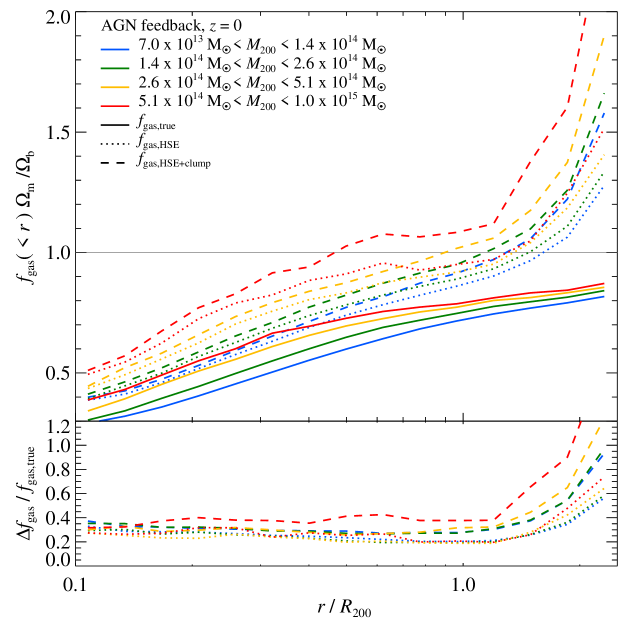
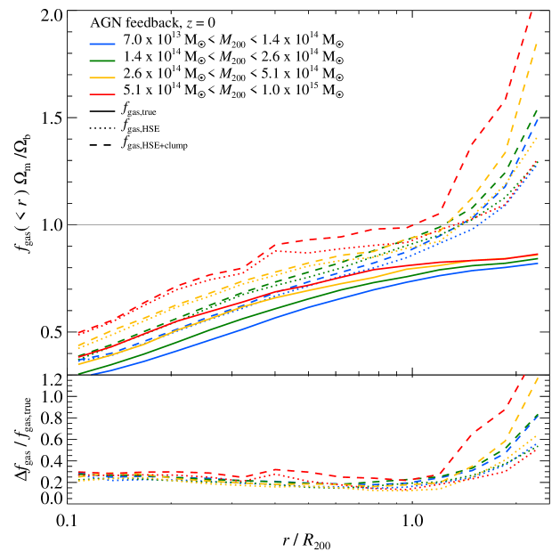
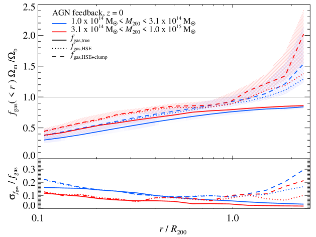
In Figure 1, we show the median enclosed gas mass fractions, as a function of radius for different cluster masses in our AGN feedback model; on the left panel for our sample of all clusters, and on the right panel for the 3rd most relaxed clusters. To define a relaxed cluster, we split the population of clusters into lower, middle, and upper bands of the ratio of kinetic-to-thermal energy, , within , which we use as a measure of dynamical state for the clusters (see Appendix A). We define the internal kinetic energy, , and thermal energy, , of a cluster as
| (1) | |||||
| (2) |
where and are the gas mass and the SPH density, respectively for all particles less than , denotes the thermal pressure (where and denote the temperature and mean molecular weight, respectively), and the kinetic pressure is defined as
| (3) | |||||
| (4) |
The code employs comoving peculiar velocities, which are translated into the internal cluster velocities relative to the overall mean cluster velocity in the Hubble flow by the relation given, where is the Hubble function, is the scale factor, () is the peculiar velocity, and x is the comoving position of each particle. The gas-particle-averaged cluster bulk flow within is and the center of mass within is . Since the most massive clusters are on average also the most disturbed systems, only two out of 25 clusters in our most massive cluster bin () meet our criterion of being a relaxed cluster, i.e., are among the lowest third when selected by the ratio of kinetic-to-thermal energy, . Hence, in order to improve the statistics of our most massive bin of relaxed clusters, we decided to also do a 3-split on in the largest cluster mass bin.
As shown in Figure 1, increases with radius and approaches values within that range from 0.8 to 0.85 (in units of ) for the mass interval from to . Smaller systems show smaller values of at every radius owing to the shallower potential wells in comparison to bigger systems. In groups and small clusters, AGN feedback is able to push the gas well beyond or halt its initial infall. In the process of hierarchical structure formation, these gas-poor groups merge to form larger clusters. Owing to their deeper potentials, those larger clusters provide a greater gravitational pull on the gas that is sitting beyond . As a result, increases at each radius in larger clusters. (We will show later on in Section 4.3 that the underlying assumption of a constant as a function of redshift at fixed cluster mass is justified in our simulations.)
These simulated values of for all cluster masses are substantially smaller than Suzaku estimates of or even 1.6 within if one accounts for a stellar mass fraction of 12% (Simionescu et al., 2011). Two sources that could potentially bias the measurement of gas fractions have been suggested, the assumption of hydrostatic masses and neglecting density clumping due to infalling (sub-)structures following the ongoing growth of clusters. Hence we will discuss each of these effects in turn.
3.1 Hydrostatic mass bias
Even if clusters are in hydrostatic equilibrium (HSE), balancing the gravitational force to the pressure gradient yields
| (5) |
Assuming that all the pressure in Eq. (5) is thermal () gives an incorrect estimate for the mass since the non-thermal pressure, in particular the kinetic pressure has to be included (e.g., Evrard, 1990; Rasia et al., 2004, 2006; Lau et al., 2009; Rasia et al., 2012; Nelson et al., 2012). For clarity we define to be the mass derived using and . We define the bias owing to the assumption of HSE as , which shows a weak increase in radius. Note that this definition differs from other approaches in the literature. Adopting results in a radially decreasing bias, presumably due to violation of spherical symmetry and non-stationary, clumpy accretion that is not accounted for in the derivation of (see Appendix B).
Comparing to the true mass inside a given radius, on average underestimates by % within (\al@2012ApJ…758…74B) and biases accordingly high (dotted lines in Figure 1). This bias is almost independent of cluster mass out to as can be seen by the fractional difference of (lower panels of Figure 1). However, individual clusters can stray from this average deviation, since each cluster has a unique dynamical state and formation history. This is suggested by a scatter of % between the and percentiles of the complete distribution (\al@2012ApJ…758…74B). For approaches that assume a constant bias, the fractional difference of would be accordingly shifted downwards (by the same factor in the lower panels of Figure 1).
When we select a sample of the third most relaxed clusters, the correction factor will necessarily be smaller. We find that the bias on for this sample is reduced to % within . In a small sample of zoomed-cluster simulations that has been selected against major mergers the hydrostatic mass correction was found to be of the order % (Kravtsov et al., 2006). However, in both cases, we see that outside , the hydrostatic bias rises steeply as approaches large values and eventually reaches equipartition around (at ) with the exact equipartition radius depending on cluster mass.
3.2 Clumping bias
The emissivity of thermal bremsstrahlung scales with the square of the gas density. Hence the X-ray-inferred gas density profile is biased high by the presence of a clumped medium (Nagai & Lau, 2011; Roncarelli et al., 2013) and attains a bias of the square root of the density clumping factor, that we define by
| (6) |
Averages are taken to be volume averages. We also define the SPH volume bias,
| (7) |
that we expect to be identical to unity everywhere. While this is the case for small radii, the SPH volume bias deviates progressively for larger radii. It reaches a negative bias of 30% at (), almost independent on the simulated physics and cluster masses, but not of redshift since it doubles at when radii are scaled to (\al@BBPS4). To obtain unbiased estimates, we decided to redefine the clumping factor, yielding
| (8) |
where the multiplication with the volume bias factor, , has been chosen to cancel the SPH volume in the weighting. Inside , the profile of increases moderately with radius but remains for for all clusters. Outside , it starts to rise sharply and reaches values of 10 at and for large clusters and groups, respectively, almost independent of the simulated physics (\al@BBPS4). At each radius, there is a clear trend of an increasing clumping factor for larger clusters, which have on average a higher mass accretion rate, i.e., they are assembling at the current epoch and hence are dynamically younger.
Cold, dense gas clumps that are ram-pressure stripped from galaxies and find themselves in pressure equilibrium with the ambient hot ICM add an artificial bias to the density clumping factor. This bias needs to be accounted for when comparing to X-ray observations by employing, e.g., a temperature cut. Hence, in our calculations of the density clumping factor, we only consider SPH particles with that can be observed by their X-ray emission.
To estimate the clumping bias of the enclosed gas mass fractions, we compute a clumping-biased density profile for each cluster by means of , and integrate this to obtain a clumping-biased gas mass profile,
| (9) |
Here, we only asses the effect of clumping bias on . In principle, density clumping should also impact the determination of . However, there are different subtle effects that may partially compensate. Those include larger Poisson scatter in density profiles implied by clumping, which then have a noisier derivative, calling for some smoothing procedure which may bias the inferred masses. Also, the X-ray emissivity is enhanced by the presence of self-bound (dense) structures which increases the logarithmic derivative of the density and hence . Conversely, these dense substructures have a lower temperature. Fitting a single temperature spectrum to the data will then bias the inferred temperature and hence low. Simulated X-ray observations are needed to carefully address these points that shall be subject to future work.
Clumping bias increases inferred values for – similar to the bias. In Figure 1, we show the effect of both biases that we denote by (dashed lines). As a result of both biases, realizes its universal value at considerably smaller radii in comparison to the true . In our sample of relaxed clusters, the universal value is reached outside whereas in our all-cluster sample, these high values are already obtained at for big clusters with . Interestingly, the biased values for increase sharply outside the virial radius, mainly driven by the clumping bias for large systems and with a substantial contribution of bias for smaller clusters. is biased high by a factor of two at for large clusters and at for groups (see Figure 1).
What is the relative contribution of these measurement biases as a function of radius and cluster mass? In our all-cluster sample, clumping bias has a small effect at the cluster center but is continuously increasing towards . At , it approximately contributes half as much as the bias to the overall bias with an absolute bias of %, depending on cluster mass. In our relaxed cluster sample, the clumping bias remains even more subdominant in comparison to the bias. However, in both cluster samples, the clumping bias increases dramatically beyond with an increasing bias with cluster mass.
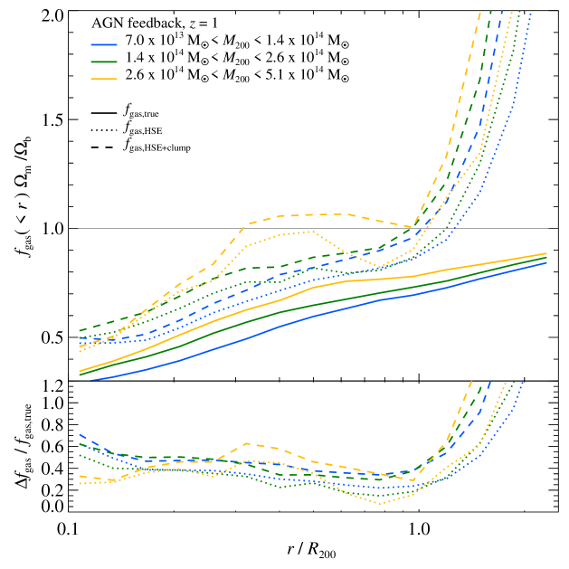
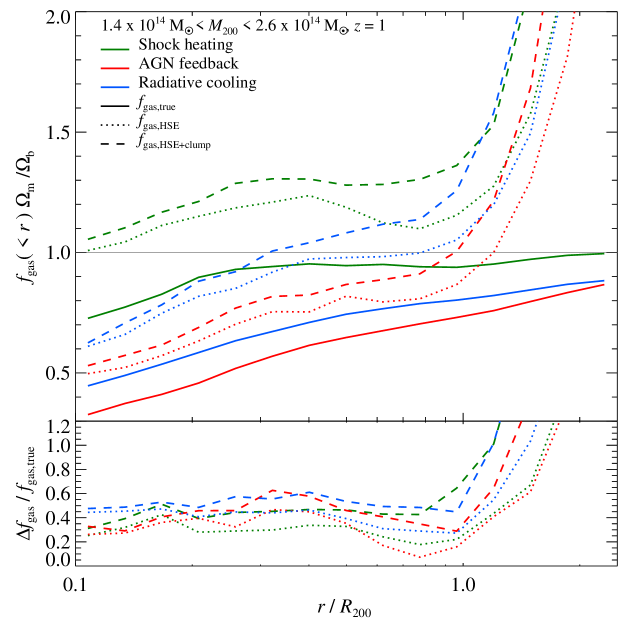
Clusters form as a result of hierarchical merging of smaller systems. Hence the kinetic pressure support (\al@2012ApJ…758…74B) and the density clumping (Nagai & Lau 2011, \al@BBPS4) increase with at fixed mass and so do the associated measurement biases of . This can be appreciated in Figure 2, which shows the radial profile of at . While the intrinsic gas mass fraction shows no significant evolution with , the assumption of hydrostatic equilibrium and of neglecting the density clumping introduces an increasing bias at in comparison to the present epoch.
All clusters:
Relaxed clusters:
Relaxed clusters, 3D:
All clusters, 3D:
All clusters, 2D:
3.3 Cluster sample variance
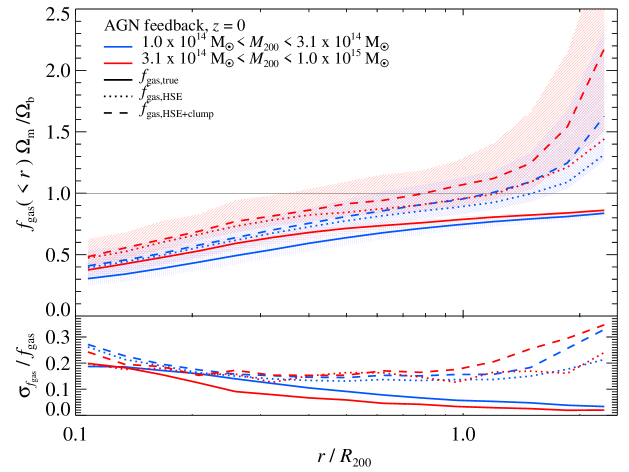
It has been suggested that sample variance of clusters could possibly account for values of larger than the cosmic mean, i.e., when a cluster experiences an ongoing merger or has close-by cluster companions. To address such questions, our large sample of clusters is ideal. It consists of 800 clusters with and has 200 clusters with keV (corresponding to ). In Figure 3, we compare the cluster-to-cluster scatter of in a sample of all clusters and a sub-sample of the third most relaxed clusters (as defined by the third of all clusters with the lowest ratio of kinetic-to-thermal energy, , within , see Equations (1) and (2)). The sample variance of the true decreases with increasing radius from a relative 1- scatter of 20% () at for our sample of all (relaxed) clusters down to at . This demonstrates the smaller influence of AGN feedback on large scales especially for big clusters where the gravity of the DM potential starts to dominate. In contrast, the scatter of the biased quantity remains fairly constant at a level of (depending on the dynamical state and mass of clusters). Within , the sample variance due to the clumping bias is negligible, but it starts to rise steeply outside , the innermost locations of accretion shocks (along filaments) that dissipate kinetic accretion energy and smooth the density distribution interior to this radius.
The envelope of starts to rise dramatically for for our all-cluster sample. This rise is shifted to somewhat larger radii for our sample of relaxed clusters (Figure 3). However, at we obtain an upper percentile of for our massive clusters () that is 30% above the universal value for our all-cluster sample and only 10% for our subsample of relaxed clusters. Cluster variance alone remains unlikely to support values that are 1.6 times the cosmic mean – the measured value at in Perseus when accounting for a stellar mass fraction of 12% (Simionescu et al., 2011, even when accounting for the moderate increase of this number by for the most massive clusters around ). Moreover, clusters that are lying outside the interval are either merging systems or are caught in a pre-merger state, properties that can easily be verified through optical or X-ray observations of the local environment of such a cluster (unless the merger axis is aligned with the line-of-sight, but such a configuration is rare and should be easily separable in a statistical sample of clusters).
3.4 Angular variance of the mass distribution within a single cluster
In nearby clusters, the large angular extent of clusters renders it impossible to cover the entire virial region of a cluster with a few X-ray pointings. Instead, a limited number of mosaic pointings along radial arms are being observed which opens the possibility of obtaining a biased answer for if there is a considerable angular variance. Two effects may play a role. First, a large mass fraction is being accreted along filaments. These anisotropic ICM features associated with large-scale structure environment suggest that the thermalization of the ICM occurs at smaller radii along overdense filamentary structures (that exert a greater ram pressure on the hot ICM) than along low-density void regions. Second, since there is a strong internal baryon-to-dark-matter density bias, a consequence of collisional-to-collisionless physics, this could in principle also lead to a significant angular variance depending on the differing efficiencies of gas thermalization and the relaxation processes of the DM component.
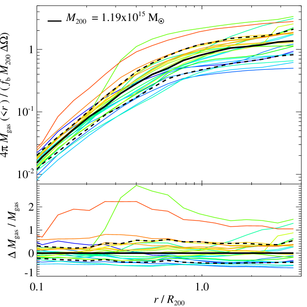
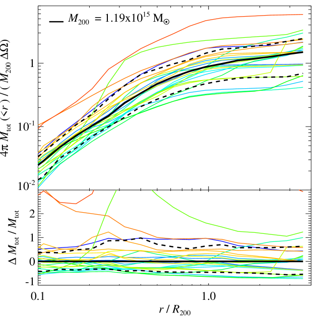
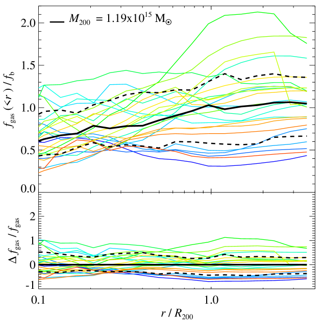
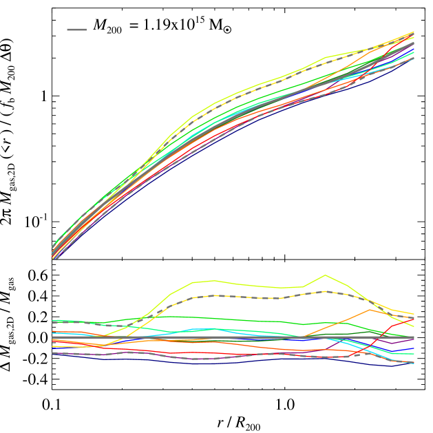
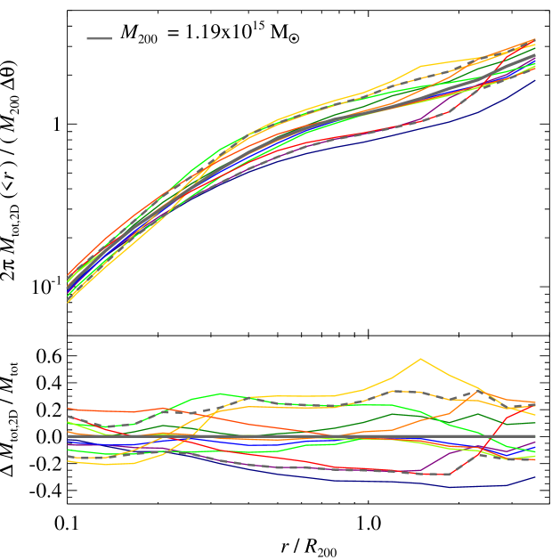
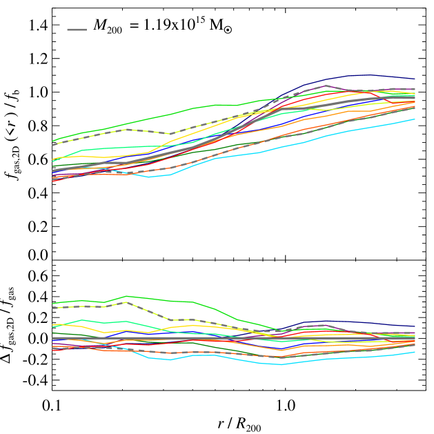
To quantify these considerations, in Figure 4 we show the profile of , , and in angular cones centered on one massive cluster of . We chose the angular directions of these 48 cones such that they subtend an equal area pixelization on the sphere (following the HEALPix scheme with ; Górski et al., 2005). The number of cones is a compromise between obtaining high-enough angular resolution to break the angular smoothing that is necessarily present in sphericalized profiles and to resolve individual substructures and cosmic filaments in these cones. At the same time, we aim at minimizing scatter due to our finite number of particles. To calculate , we sum up the mass distribution of the gaseous, stellar, and DM components in those cones.111For the gas component, we sort the volume fraction of an SPH smoothing kernel into the corresponding radial bins, but neglect the extension of the smoothing kernel in angular directions for performance reasons (see Appendix C.
We observe considerable scatter in all three distributions, , , and , depending on the angular direction. There are a few enormous outliers in the and cones, deviating upwards up to a factor of 3 from the median (shown with solid black) in the case of and even beyond for . The right-most panel in Figure 4 shows that in the most extreme cases, the cone profiles of can be biased high by a factor of two in such a massive cluster with , potentially providing an explanation of the boosted values of reported in the north-western arm in Perseus (Simionescu et al., 2011). Care should be taken when interpreting these values in cones, since projection effects may lower these values. However, as demonstrated in Figure 1, hydrostatic mass bias as well as density clumping may (partially) compensate for these projection effects.
Only in the cones, those outliers can be seen down to small radii which is expected as DM substructure only obeys collisionless physics that allows substructures to penetrate deep into the halo without too much affecting the dense central subhalo structures by tidal stripping. In contrast, the gaseous content has been removed by means of shocks or ram-pressure stripping at larger radii, lowering the variance of at smaller radii (see Figure 4). These large outliers are absent in the distribution of cones, which implies a smaller variance (dashed black). This suggests that these outliers are caused by self-bound substructures that are still holding on to (some) of their gas at larger cluster radii, i.e., there exists a tight spatial correlation of the DM and gas distribution (see \al@BBPS4 for a detailed analysis).
Line-of-sight projection smoothes out the largest angular variations in the 3D distribution. We calculate projected (cylindrical) mass distributions according to
| (10) | |||||
| (11) |
where denotes the length of the simulation box. Before projecting, we smooth the discrete stellar and DM masses by distributing their individual masses according to an SPH-type smoothing kernel that extends up to the nearest 48th neighbouring particle (of the same type). In Figure 5, we show the resulting projected profiles of , , and in 12 equally large angular sectors, centered on the same massive cluster as studied in Figure 4. In comparison to the 3D cones, the scatter is smaller and there are less dramatic outliers in the projected sector distribution of , , and . Unlike the 3D case, the largest 2D outlier sector in this cluster does not exceed far above the cosmic mean of within .
In Appendix D, we show that the variance of projected sectors of and depends only very weakly on the number of sector elements, hence justifying our choice of 12 elements. Instead, the scatter of the X-ray luminosity strongly depends on the number of sector elements, especially in SPH simulations (see Figure 4 of Vazza et al., 2011b). Presumably, this increased scatter solely derives from the increased clumping factor with radius. The increased scatter in the SPH simulations in comparison to AMR simulations especially for (Vazza et al., 2011b) may stem from an incomplete clump removal.
3.5 Variation of the mass distribution with angle across cluster samples
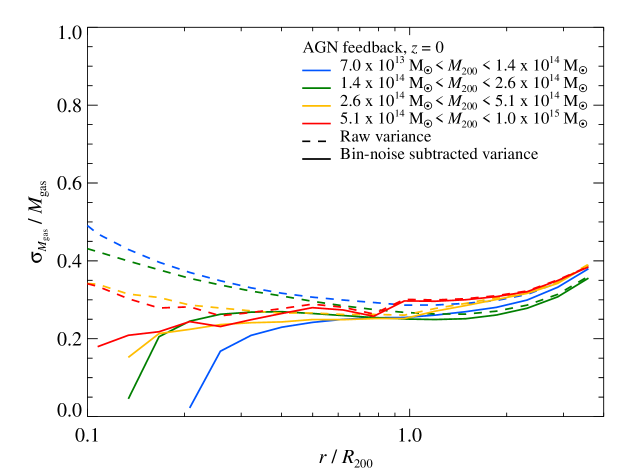
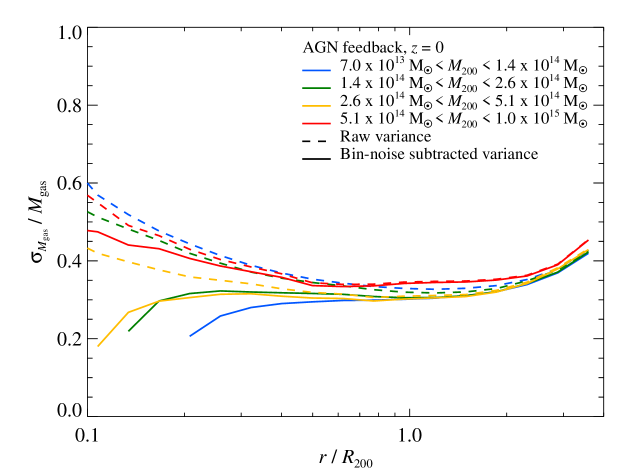
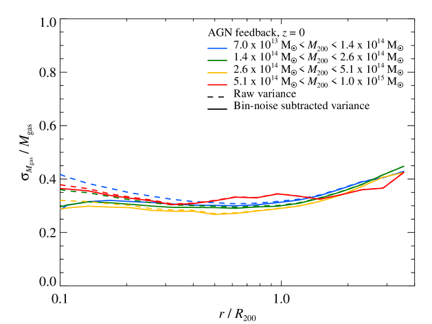
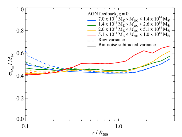
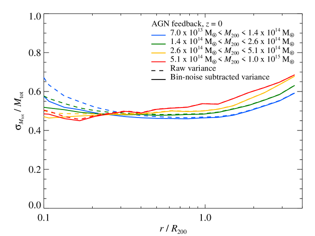
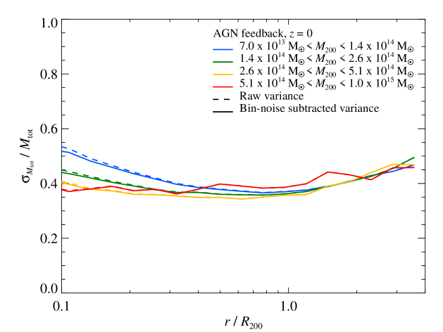
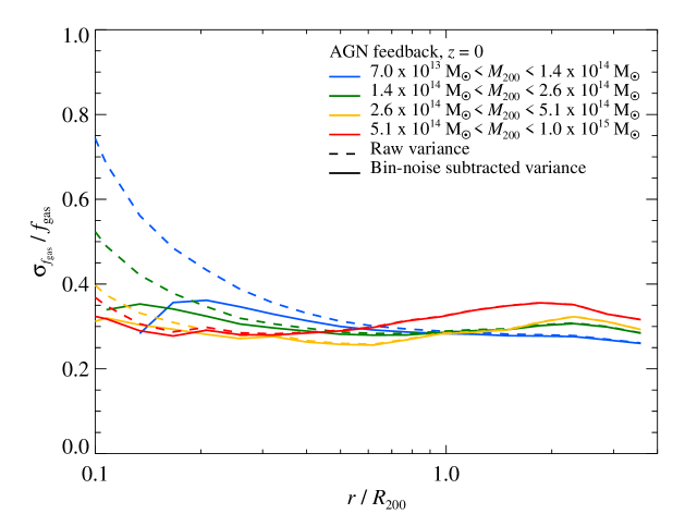
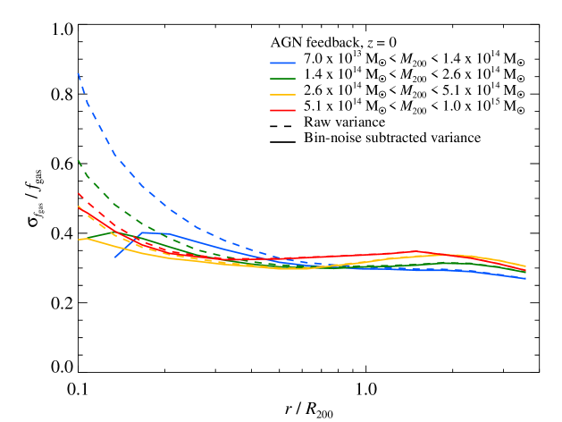
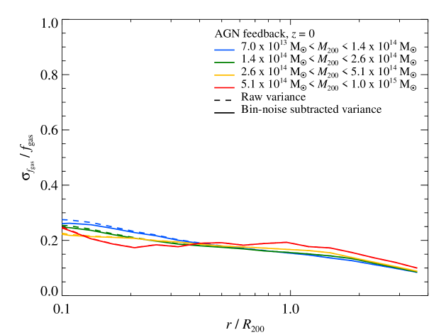
In order to obtain statistically valid answers on how this scatter across different cones varies among our cluster sample, we first compute the variance of the profiles of , , and across 48 angular cones (dashed lines in Figure 4) for all clusters. Since the distribution within a single cluster is non-Gaussian and positively skewed (by the presence of substructures), we define the angular variance of , , by the difference of the upper and lower percentiles, normalized by twice the median of . In the top panels of Figure 6, we show the mean of across our cluster sample (color coded by cluster mass). The same quantity is being calculated for and (lower panels of Figure 6) across a sub-sample of the third most relaxed clusters (left) and across all clusters (middle). Also shown is the mean of the angular variances , , and for the projected 2D maps (right).
:
:
As shown in Figure 6, there is an upturn of the raw 3D variances (dashed) visible at small radii and in particular for galaxy groups. This is caused by the noisy distribution of a comparably small number of SPH particles in the central cluster regions in combination with the smaller radial bin size of our logarithmic equally-spaced grid towards the center, when distributing the particle masses among the angular cones. As a result of the mutual repulsive hydrodynamical forces of neighboring SPH particles, they maintain a sub-Poissonian distribution with repulsive short distance correlations on scales of order the corresponding inter-particle separations. The full characterization of such a distribution with dynamical evolution of SPH is not possible in terms of known distributions. Hence we decided to cap this numerical noise contribution by treating it as Poissonian and subtract a Poissonian noise term in quadrature from the raw 3D angular variance. We caution that this over-corrects the intrinsic variance at small radii, causing an artificial decrease of the bin-noise subtracted variance (solid). We emphasize that our focus here is on large scales with (where the range corresponds to large and small clusters, respectively). Those scales are not subject to this numerical limitation. Hence in order to improve upon our analysis in the central regions, an increase in numerical resolution would be needed. The 2D angular variances in the central regions are only little affected by the sub-Poissonian variance due to the sufficiently large number of particles that are projected onto the central regions.
Inside , the 3D angular variance of does not strongly depend on mass and reaches values around 30% at with a moderate increase at larger radii. In contrast, the 3D angular variance of is steadily increasing and reaches values around , depending on cluster mass (with the upper range indicating larger clusters that are on average dynamically younger). These values are only moderately reduced by percentage points for our relaxed cluster sample. The different 3D angular variances of and can be understood by the collisional nature of the gas that is able to dissipate part of its kinetic accretion energy more efficiently (through shocks and ram-pressure stripping of the gaseous contents of substructures), thereby reducing its 3D angular variance. This is in contrast to the collisionless DM component (dominating the total mass) which shows a larger 3D angular variance of its mass distribution.
Interestingly, the Poisson noise-corrected 3D angular variance of remains almost constant with radius at the level of not only within the clusters but also for . Furthermore, depends very weakly on cluster mass. Both of these properties can be understood by the fact that at these large radii, most of the accreting substructures have not yet passed the accretion shock nor are they affected by ram-pressure stripping as they still move through the dilute warm-hot inter-galactic medium. Hence these self-bound substructures are still holding on to their gas, implying large spatial correlations of the DM and gas distribution (see also Figure 4 and \al@BBPS4).
The most striking feature of all our Poisson noise-corrected 3D angular variances is the rather constant behavior with radius, in particular for the 3D angular variances of and , as well as the moderate radial increase of that of . In principle, the mass distribution in cones allows for finer sampling of the cluster shape beyond the moment-of-inertia tensor and is sensitive to higher-order moments – a measure that would be similar to density clumping for sufficiently high multipoles. In practice, this is limited by the Poisson noise due to our finite particle resolution. Moreover in Figure 6, we concentrated on the radial profiles of the second moment of the 3D angular variance which is intimately related but not identical to cluster ellipticities as obtained through eigenvalues of the moment-of-inertia tensor as a function of radius (\al@2012ApJ…758…74B). The ellipticity of the gas density also shows a constant behavior inside while it is rising at larger radii. In contrast, the DM ellipticity shows already a moderate increase with radius which only starts to rise more steeply outside (\al@2012ApJ…758…74B) – very similar to our findings for the 3D angular variance of that is dominated by DM.
When averaged over sufficiently large scales, i.e. at very large radii, is expected to assume the cosmic mean and the 3D angular variance should approach zero. In our case, the outermost radial bin is centered on and has a radial extend of . The volume associated with that cone bin is for a cluster with Mpc. This volume is still small in comparison to the scale associated with the root mean square variance of linear theory in spheres of radius , . In fact, the 2D angular variance shows the expected downturn for radii . The volume associated with the outermost 2D radial bin of a cylindrical projection length of is for a cluster and . This volume is 60 times larger than for the corresponding 3D case, but still somewhat smaller than the volume of a sphere with radius . Why do we then observe a decline in the 2D angular variance? This is because the line of sight projection averages over many uncorrelated patches on scales , which draws down for larger radii and brings back to the cosmic mean. In the 3D case, the considerably smaller volume and the inherent radial correlations of the gas and DM distributions on these scales (as quantified in \al@BBPS4) explain the flat radial profile of out to .
All angular variances of and (2D and 3D) show an increase at the largest radii (). This reflects the increase of the root mean square variance, , on these scales due to the dominance of the two-halo term in halo-mass cross-correlation, which corresponds to the mass autocorrelation function with a mass-dependent offset in amplitude known as the halo bias factor (Hayashi & White, 2008).
4 Gas and stellar mass fractions in cosmological simulations
Here, we present results on how varies with simulated physics, radius, cluster mass, and redshift. These results are summarized in Table 1 and 2.
4.1 How different physics determines and
:
:
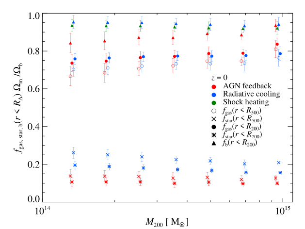
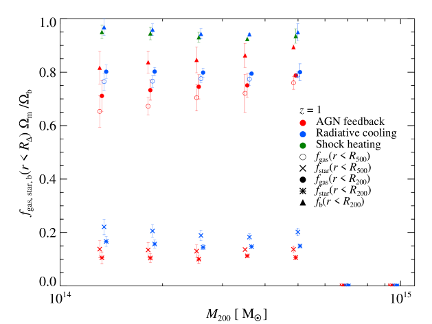
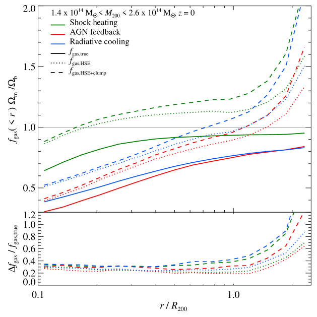
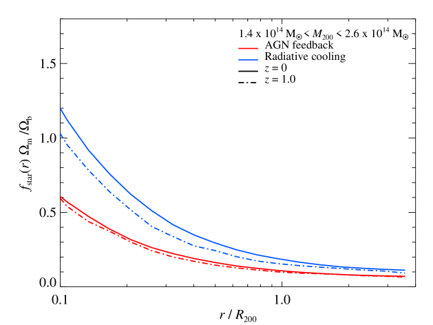
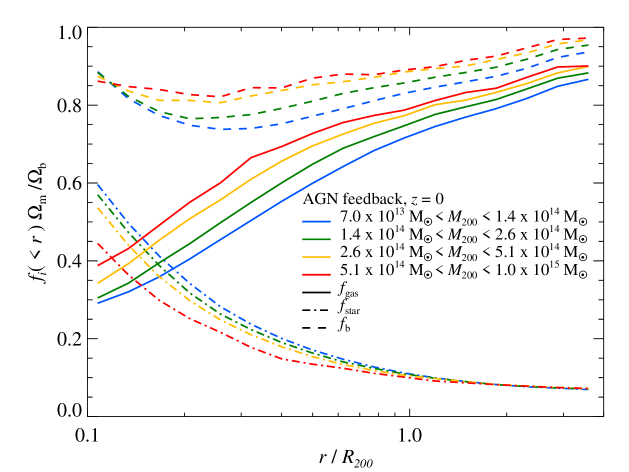
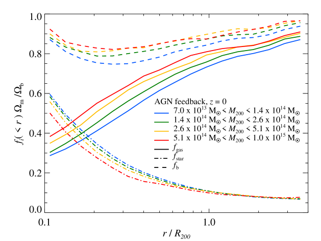
Even though we believe that our AGN feedback model represents the closest approximation to reality, it is important to compare it to simpler physics models, which have been extensively studied in earlier literature. Moreover, there is considerable uncertainty about the correct physics underlying AGN feedback so that trends relative to our simpler models can be very instructive. Hence, we compare how different physics models impact the radial profiles of (Figure 7) and (Figure 8). This is supplemented by a figure demonstrating the cluster mass dependence of and within and for differently simulated physics (Figure 9).
In our shock heating-only model, approaches a value of in units of at (which is reduced by one percentage point for larger clusters). Outside the virial radius, is continuously rising to asymptote to the cosmic mean only at . This may be partially due to a transfer of energy from DM to the gas during group/cluster mergers. In an equal mass collision, SPH simulations show that the DM can transfer up to 10% of its energy, and even a 10:1 merger may be able to reduce the DM energy by a couple of percent (McCarthy et al., 2007). There is also the possibility that some of this gas deficiency may be related to the SPH technique that we use here. There appears to be a discrepancy to adaptive mesh-refinement simulations that find higher values of within (Kravtsov et al., 2005, see also Section 4.5, for a detailed discussion). At small radii, the shock-heated ICM provides pressure that causes the inner slope of the gas density profile to be rather flat, while the collisionless DM exhibits a cusp (e.g., Gao et al., 2012). As a result, this causes a decreasing gas fraction inside the DM scaling radius, i.e., for .
Our models with AGN feedback and radiative cooling have similar values of at , in particular for . However, in the AGN feedback model, only marginally evolves with , while it increases for higher in the case of radiative cooling and star formation. This also manifests itself in the constant evolution of the profile in the AGN feedback model. In contrast, the stellar mass is increasing with time in the radiative model without AGN feedback due to the well-known overcooling problem in cosmological simulations of galaxy clusters if cooling is not counteracted by any feedback process (e.g., Borgani & Kravtsov, 2009).
For , the values of in different radiative models (as well as for different redshifts) approach each other. However, in comparison to our shock heating-only model, there is still a gas mass deficit of 10% at . In the raditive cooling model, the stellar mass fraction makes up for this deficit (Figure 8) while in the case of AGN feedback, stellar mass fractions are reduced by a factor of in comparison to our radiative cooling model. (Note that in our radiative cooling models depends on numerical resolution as this model is physically not converged.) The remaining gas mass has been pushed to even larger radii through the action of AGN feedback (McCarthy et al., 2011). Interestingly, these lower values for in our radiative models in comparison to our non-radiative models imply a temperature increase in the outer parts (e.g., Figure 4 of Fabjan et al., 2010) that is necessary to balance the gravitational cluster potential.
At , all our models show approximately a similar relative bias (left bottom panel of Figure 7) while the relative differences with respect to the true are larger at (right bottom panel of Figure 7). However, there are some notable differences. At large radii, the radiative cooling model exhibits the largest bias, while our AGN feedback model shows the lowest bias. This is presumably due to AGN outflows depositing heat at these large radii (early on) which manifests itself in an increased pressure in comparison to the radiative cooling model (Battaglia et al., 2010). This increased thermal pressure moves the average location of accretion shocks to larger radii (since these form at the location where ram pressure due to infalling gas balances the thermal pressure of the ICM), which causes a deceleration of the accreting material already further out, and hence slightly decreases the average kinetic pressure support in the AGN feedback model. Hence, the bias corrections shown in Figure 1 are conservative given that the AGN feedback model shows an overall lower bias in comparison to the other models.
At , the bias due to the hydrostatic equilibrium assumption and as a result of neglecting clumping () is rather constant inside and shows values around 30%. At higher redshifts, , increases to a level that fluctuates around 50%. Outside the virial radius, the bias increases sharply, albeit at a slightly slower rate in our AGN feedback model for reasons explained above. The location of the sharp increase in the bias moves from (at ) to (at ). This is mostly due to the definition of and can be approximately aligned by changing the definition to , which compares the average interior density to the mean mass density rather than the critical density of the Universe (Figure 21 of \al@2012ApJ…758…74B, ).
All clusters:
Relaxed clusters:
4.2 Gas and stellar mass fractions across cluster masses
How do the gas and stellar mass fractions, and , as well as the sum of both, the baryon mass fraction, , vary with cluster mass? In Figure 9, we show and for our 3 different physics models as a function of cluster mass. As discussed in Section 4.1, our model that only accounts for shock heating approaches a value of () at (which is reduced by one percentage point for larger clusters). These lower values of represent the pivot point from which our radiative models can reduce furthermore through conversion of baryons into stars or by expelling it from the cluster region (in the case of our AGN feedback model).
In our radiative cooling model, increases moderately with cluster mass at to level off at a value of for big clusters. This trend is weakened at . The opposite behavior is seen for so that the resulting baryon fraction almost exactly sums to a value that is seen in our shock heating-only model. At , the scatter in drops by percentage points in comparison to the scatter at for both of our radiative models.
While in our AGN feedback model, the effect of a decreasing towards lower cluster masses is amplified and the trend of an increasing towards lower masses is weakened (at ). Figure 10 shows that these trends are still present at smaller radii and become progressively stronger towards the center. Interestingly, these effects partially compensate for the baryon fraction, , which attains a much weaker mass dependence. Comparing the radial profiles of these mass fraction for all clusters (left panel of Figure 10) and a sub-sample of the third most relaxed clusters (right panel) we virtually do not see any differences. In contrast to our non-equilibrium measures such as clumping or kinetic pressure support, the mass fractions in gas, stars, and baryons are almost independent on the clusters’ dynamical state. The only exception are the central values for in massive clusters which are higher by 5% in our relaxed-cluster sample in comparison to all clusters.
However, there are two noticeable differences of the mass fractions in our AGN feedback model in comparison to those in our radiative cooling model (Figure 9). (1) The baryon fractions do not sum up to the value of our shock heating-only model. There is a deficit of gas mass at that decreases from 10% at down to 5% at . Only for the largest clusters () does the baryon fraction of the AGN feedback model correspond to that of the shock heating-only model. As explained in in Section 4.1, this is due to the powerful outflows of gas that deposit considerable amounts of gas beyond so that the cosmic mean is not even reached by . The only exception to this are the largest clusters whose gravitational potential provide a strong enough pull on the gas that was successful in having re-accreted the gas. (2) In our AGN feedback model at , remains almost independent of cluster mass (in contrast to the values at ).
This behavior is very interesting with respect to its implications for the redshift evolution of on group scales. In order to build up high-mass clusters with low values of , their progenitors also had to have these low stellar mass fractions in a hierarchically growing universe since the amount of baryons locked up in (low-mass) stars remains there throughout a Hubble time in the model of star formation adopted here (Springel & Hernquist, 2003).222There can be return of stellar mass to the gaseous phase by means of stellar winds which is thought to mostly sustain star formation in galactic disks (Martig & Bournaud, 2010; Leitner & Kravtsov, 2011). If there is a considerable population of intracluster stars (Puchwein et al., 2010), stellar mass loss could be a potential channel of increasing at the expense of , but the low observed mass fraction of intracluster stars renders it unlikely to be an important contribution, especially on the high-mass cluster end (Lin et al., 2003; Zibetti et al., 2005; Gonzalez et al., 2005, 2007; Giodini et al., 2009). Since is increasing towards lower cluster masses in our radiative cooling model, this would imply that the groups we observe today, do not reflect the properties of groups at high- (in terms of ) that merged to assemble large clusters today. This is demonstrated by the almost constant behaviour of as a function of cluster mass at in our radiative cooling model (right-hand panel of Figure 9). The values of in groups at is almost at the same level as for big clusters today. In contrast, the approximate constancy of with cluster mass in our AGN feedback models suggests that groups that are observed today do not need to be different from group-scale progenitor systems of clusters today.
The increasing value of with time on groups scales in our
radiative cooling model (Figure 8) also suggests an excess
star formation at late-times which results in too blue colors and too massive
stellar masses at the high-mass end in comparison to observations
(Sijacki et al., 2007). We note that the distributions of
and are almost Gaussian (independent of the models), resulting in
almost identical median and mean.
4.3 Redshift evolution of gas and stellar mass fractions
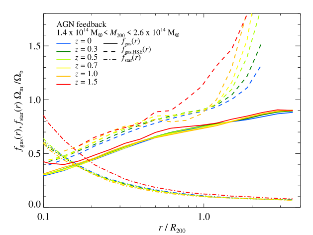
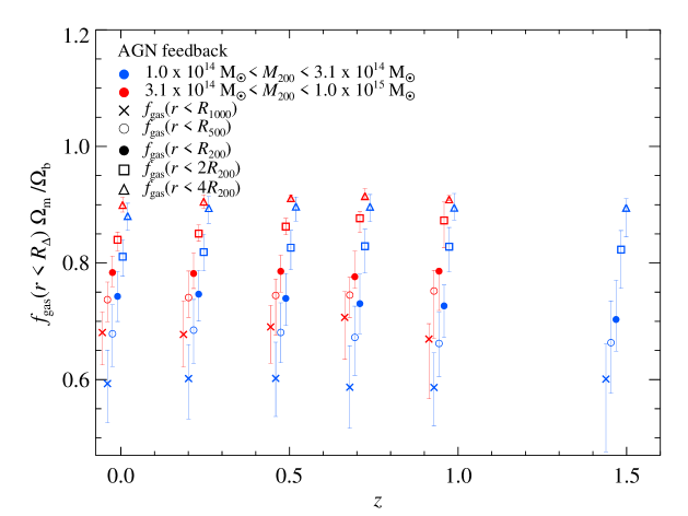
First, we show the redshift evolution of the median profiles of the stellar and gas mass fractions in our AGN feedback model at fixed cluster mass, (Figure 11). To address the cluster-to-cluster scatter, we additionally show the redshift evolution of the median and percentiles containing 68.3% probability centered on the median (corresponding to 1- intervals) for small and big clusters separated at the characteristic mass of (Figure 12).
For a given cluster-mass bin and with increasing redshift, we are probing clusters with a higher mass accretion rate on average, i.e., dynamically younger systems. Back to , there is almost no evolution in these mass fractions, especially for bigger clusters and larger radii. The constancy of implies that the integral of the galaxy mass function increases at the same rate as the DM mass, which is realized if most of the stellar mass is already in place by the time it assembles in the cluster halo (since we do not account for stellar mass loss in our simulations).
How does this finding compare to observations? Optical observations find an abundance of red elliptical galaxies within clusters that is the foundation for the red sequence cluster finding algorithm (Gladders & Yee, 2000). This is the standard cluster finding method in the optical for and has been extended to higher redshifts by the Spitzer Adaptation of the Red-sequence Cluster Survey (SpARCS, Muzzin et al., 2009) and photometric cluster finding techniques such as the IRAC Shallow and Deep Cluster Surveys (ISCS and IDCS, Brodwin et al., 2006; Mancone et al., 2012). In the literature there is a controversy about the faint-end slope of the red sequence, which translates into an uncertainty of the built-up of stellar mass in observations across cosmic time. Some groups find a constant faint-end slope of the red sequence (e.g., Stanford et al., 1998; Andreon, 2006, 2008; De Propris et al., 2013) after accounting for surface brightness selection on red sequence luminosity function while others observe a decrease of the faint end of the red sequence (De Lucia et al., 2004, 2007; Tanaka et al., 2004; Stott et al., 2007; Gilbank et al., 2008; Rudnick et al., 2009; Papovich et al., 2010; Vulcani et al., 2011; Rudnick et al., 2012). Those authors infer an evolving faint end of the red sequence, which they interpret as a built-up of stellar mass in the red sequence with a stellar mass growth by factor of two between down to 0.6 and another factor of two since then. This agrees on average with the mass assembly history of cluster halos after accounting for stellar mass loss.
In our simplified star formation models, we do not account for stellar mass loss, which can return up to to the ambient medium, depending on the initial mass function. We emphasize that even if our stellar mass prescription and hence may be off by 50% due to the effect of stellar mass loss or limiting resolution, this would bias the gas mass fractions by a factor of at most . However, this factor will be substantially reduced in practice because a larger (smaller) amount of formed stellar mass is partly balanced by an increased (decreased) inflow of gas from larger radii to maintain the approximate pressure balance due to the increased gas mass loss to stars. This renders our results with respect to quite robust.
We demonstrate in Figure 12 that there is weak evolution of (at the level of 1-) for our small clusters at which disappears for larger radii or larger clusters. In particular for clusters with , we see no evolution of the median already for radii as small as . At , both and are increased towards the center indicating that those redshifts probe the tail end of the epoch of our AGN feedback which is most efficient at in blowing gas out (Figure 11, see also McCarthy et al. 2011). At , we run out of statistics for the mass range under consideration. However, this interpretation is confirmed by looking at a smaller cluster mass range at an even higher redshift which shows a further increase in the stellar mass fraction.
This finding is also consistent with the amount of energy injected by AGN feedback over the simulation time. Approximately one third of total energy is delivered in the cluster formation phases at (analogous to high- quasar-like feedback), another third in the redshift range , and the final third below (analogous to jet/bubble like feedback). These fractions depend moderately on the numerical resolution; increasing the resolution enables to resolve the growth of smaller halos at earlier times and causes a higher fraction of energy injection at higher redshifts (see Battaglia et al., 2010, for a discussion).
Despite the almost constant evolution of the gas fractions for , there is positive evolution of the biased gas mass fraction at these radii due to the evolution of the kinetic-to-thermal pressure ratio when radii are scaled to (Figure 11). Most of this apparent evolution can be absorbed by redefining as the radius at which the mean interior density equals times the mean density of the universe (see Figure 21 in \al@2012ApJ…758…74B, ). However, this rescaling would then imply a redshift evolution of with smaller values of at higher redshifts.
4.4 Comparison to data
Data comparison of radial profiles:
Data comparison of enclosed mass fractions:
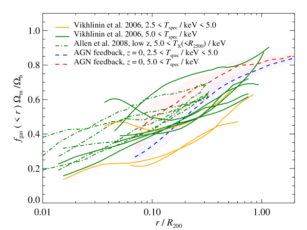
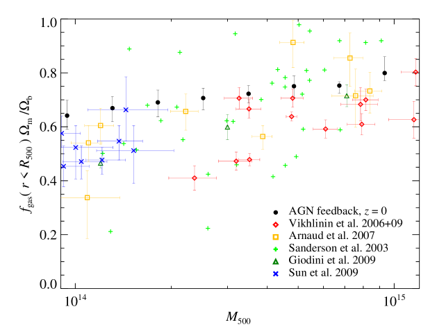
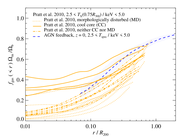
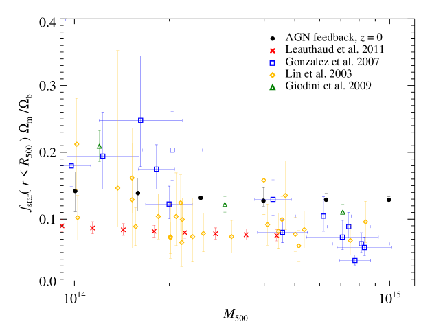
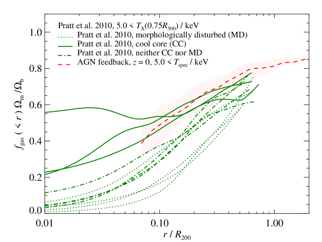
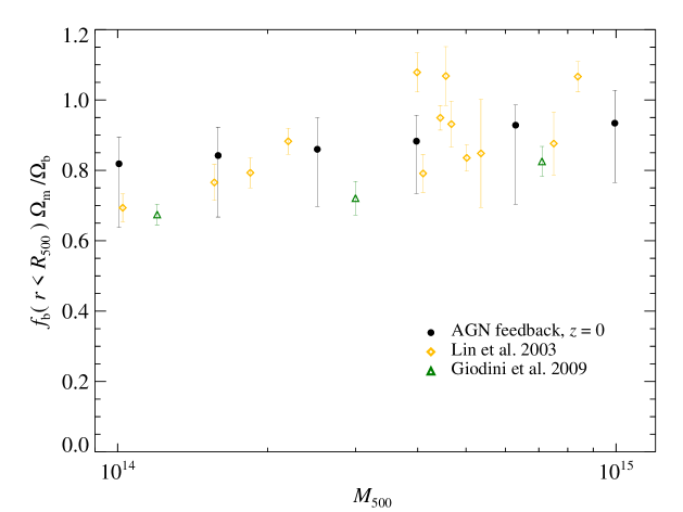
In Figure 13, we compare our AGN feedback model with data. We compare radial profiles of clusters that are sorted in two bins according to their spectroscopic temperatures, and . We use the relation by Vikhlinin et al. (2009a) to translate our values to spectroscopic temperatures. We adopt a 15% correction to the X-ray-inferred estimates (Kravtsov et al., 2006), which is valid for the respective observational sample selection criterion. Thus, the spectroscopic temperatures 2.5 keV and 5 keV correspond to and , respectively.
The left panels of Figure 13 show gas mass fractions from individual X-ray cluster observations that combine surface brightness and temperature maps of deep Chandra (Vikhlinin et al., 2006; Allen et al., 2008) and XMM-Newton data of a representative sample of nearby X-ray galaxy clusters (REXCESS, Pratt et al., 2010).333We separate the XMM-Newton clusters additionally into cool core and morphologically disturbed systems. The cool core definition is based on scaled central density, and the morphologically disturbed definition is based on centroid shift, , following Pratt et al. (2009). The two clusters that are classified as both cool core and morphologically disturbed systems, are presented as being morphologically disturbed. There is generally good agreement of our model clusters populating the high-temperature bin, especially with the Chandra data. In contrast, our simulated small-mass clusters tend to have on average slightly too high values. However, these Chandra data represent a biased sample since Vikhlinin et al. (2006) and Allen et al. (2008) targeted extremely relaxed cool core clusters for their mass measurements. REXCESS, on the other hand, should be unbiased for X-ray selected systems. Indeed, our model profiles compare similarly well to the REXCESS cool core systems while we overproduce the apparent estimates in morphologically disturbed systems (independent of cluster mass respectively spectroscopic temperature). It is unclear whether the cause for the discrepancy is on the data or simulation side. There is the possibility that our simulations fail to reproduce the non-cool core systems while they apparently match the characteristics of cool core systems. However, statistically, we find no evidence that the true is considerably changed as a result of the cluster’s dynamical state (Figure 1). On the other side, it remains to be seen whether spherical profiles of these inherently non-spherical merging systems bias the derived values for low.
In Figure 14, we compare our models with estimates from the combination of Planck Sunyaev-Zel’dovich data and different X-ray observations of massive clusters (keV). Depending on the availability of X-ray spectra, different approaches have been pursued in the literature. The Planck collaboration used XMM-Newton data interior to with spectroscopic temperature profiles (Planck Collaboration et al., 2013b) and extrapolated these beyond while assuming two hypotheses that are likely bounding the true profile.444Note that we use an updated version of as presented by the Planck Collaboration et al. (2013c). In combination with deprojected Planck pressure profiles, this yields gas density profiles and—through integration—. The total mass profile is assumed to follow a generic NFW model (Navarro et al., 1997), which is normalised to from the scaling relation (Arnaud et al., 2007, 2010). The resulting profile is somewhat lower than that of our AGN simulations for while it agrees with the simulation model at larger radii. Since our simulated pressure profiles match the observed ones (Planck Collaboration et al., 2013b), the reason for the discrepancy could either lie in the assumptions used to derive or that our simulations yield too high values for . Possibilities for observational biases include incomplete accounting for multi-temperature phases in cluster outskirts and biases of the total mass profile. could be biased by neglecting the substantial scatter among individual DM density profiles as well as not accounting for the covariances between the different parameters adopted for the DM profile such as mass-concentration and scaling relation.
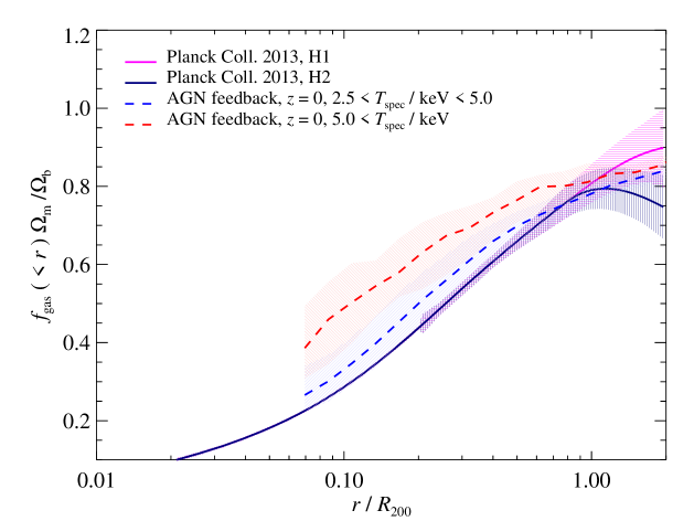
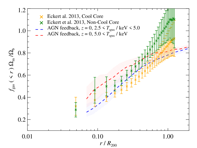
Using ROSAT data (that lacks spectroscopic X-ray information) of a sample of 18 clusters that also has Planck Sunyaev-Zel’dovich data, Eckert et al. (2013) follow a different methodology. This uses the hydrostatic equilibrium mass,
| (12) |
where derives from the X-ray emission measure and is subject to residual density clumping (that escaped the masking in the X-ray analysis). The thermal pressure gradient is obtained from the Planck best-fit generalized NFW models for the pressure, which does not depend on clumping. The gas mass fraction is derived via , where is given by Equation (9). Hence, the gas mass fraction obtained by this method scales approximately with the (residual) clumping factor,
| (13) |
rather than the square root as in the case of pure X-ray based analysis (where the pseudo pressure scales also with the residual , canceling the clumping factor dependence in ). Additionally, is biased high owing to the hydrostatic mass bias, i.e. by neglecting the kinetic pressure support (see Figure 1 or Rasia et al. (2006); Vazza et al. (2011a); Nelson et al. (2012)) and the non-thermal pressure contributed by a potential relativistic particle population in cluster outskirts (Pfrommer et al., 2007; Pinzke & Pfrommer, 2010; Vazza et al., 2012). As before for the individual Chandra and XMM-Newton clusters, our simulation models provide a good match to the median of six cool core systems by Eckert et al. (2013). However, their median profile of twelve non-cool core clusters shows larger values than predicted by our simulations for radii . This is especially remarkable since there is a substantial discrepancy between the non-cool core systems in the sample by Eckert et al. (2013) and the morphologically disturbed systems of Pratt et al. (2010), some of which may be explained by the different dependencies on the clumping factor as discussed here. We caution that more careful X-ray mocks (exactly quantifying the various biases discussed here) are needed to draw final conclusions regarding the direct comparison of our simulated models with observations.
In the right-hand panels of Figure 13, we compare the cluster mass dependence of enclosed gas mass fractions (top), stellar mass fractions (middle), and baryon mass fractions (bottom). Note that we only use those compilations of versus mass where the gas and stellar masses have been obtained from the same clusters, respectively. Overall, our AGN feedback model successfully reproduces observed values and trends, albeit with slightly higher values of (and to a lesser extent ) at the mass scales of groups in comparison to X-ray observations (cf. Arnaud et al., 2007; Sun et al., 2009). While the scatter of our simulated distribution is noticeably smaller, we caution that we did not include measurement biases that would substantially add to the simulated scatter as demonstrated in Section 3.
There could be several explanations for an overshooting of our simulated values at group scales. Those could include numerical resolution, shortcomings of the AGN modeling, or missing physics in the simulations. Increasing resolution would enable us to resolve the formation of smaller objects earlier on which may allow a more vigorous blow-out of the gas already in halos in the mass range . Those are just above the knee of the galaxy luminosity function and hence have a decreasing efficiency of star formation per unit halos mass in more massive halos which is usually attributed to AGN feedback (e.g., Bower et al., 2012; Puchwein & Springel, 2013).
As laid out in Section 2, we use an extremely low-resolution incarnation of AGN feedback that enables us to simulate large volumes and cluster samples, which are needed to provide precise predictions for the next generation X-ray and SZ surveys. Our AGN feedback prescription couples the thermal energy feedback to the global SFR of the central cluster region. While this model is able to arrest overcooling in massive clusters, it may be too simplified for groups. The observed (low-frequency) radio emission that spatially coincides with X-ray cavities suggests the presence of non-thermal components composed of cosmic rays and magnetic fields in these lobes. Modelling AGN feedback into cosmic ray rather than thermal energy (Sijacki et al., 2008) or exploring kinetic jet feedback that thermalizes at larger radii (Dubois et al., 2010) may be viable alternatives to our simulated scenario, but would also require better spatial resolution. If cosmic rays are injected into the ICM by the break-up of radio bubbles due to Kelvin-Helmholtz instabilities, they can stream at the Alfvén velocity with respect to the plasma rest frame and heat the surrounding thermal plasma at a rate that can balance that of radiative cooling on average (as demonstrated for the Virgo cluster), thereby providing a physical solution to the “cluster cooling flow problem” (Loewenstein et al., 1991; Guo & Oh, 2008; Pfrommer, 2013).
Finally, our model may be missing important physics that could additionally add entropy to the centers of groups, such as the recently suggested (Broderick et al., 2012; Chang et al., 2012; Pfrommer et al., 2012; Puchwein et al., 2012) blazar heating model that proposes the bolometric luminosity of TeV blazars as an additional heating source of the inter-galactic medium. Phenomenologically, highly biased regions that first turn-around to form groups and clusters should be heated first. This would imply an evolving pre-heated entropy floor and cause an additional decrease of in late-forming groups that are observed on a sufficiently short time scale after formation so that the central group medium had not have time to enter the strongly cooling regime (Pfrommer et al., 2012).
4.5 Comparison to previous work
Given the importance of cluster X-ray observations for cosmological parameter estimation, there has been a comparably large body of work concerning gas fractions in cosmological cluster simulations. Early work on in non-radiative simulations showed a strong systematic discrepancy between different numerical methods. This is surprising since all codes should solve the same equations for the gas and collisionless DM physics without any ambiguity in formulating a subgrid description of star formation and associated feedback processes. SPH simulations of ten massive clusters in a CDM cosmology derived values of and 0.83 within and , respectively, and show only a very weak evolution of from to 0 (Eke et al., 1998). A number of further studies that all employ the energy formulation of SPH confirm these findings (Frenk et al., 1999; Bialek et al., 2001; Muanwong et al., 2002). In contrast, cluster studies that employ the adaptive mesh refinement (AMR) technique for solving the hydrodynamic equations find higher values of and within and , respectively (Kravtsov et al., 2005). Cluster simulations with the entropy-conserving SPH code GADGET yield values of , higher by about 5 percentage points than the energy-conserving formulation of SPH but still smaller than the AMR results (see Kay et al., 2004; Kravtsov et al., 2005, which is also in line with our findings). All the different methods find no significant redshift evolution of the baryon fraction in non-radiative simulations.
Simulations with radiative cooling and star formation necessarily yield larger discrepancies in the resulting values owing to the larger uncertainties of implementing subgrid star formation and feedback processes. Common to all of these approaches is that too many stars condense out of the ICM, which results in the “overcooling problem”, i.e., values that are too small and values that are too high in comparison to observations. SPH simulations (employing the energy formulation) with radiative cooling or feedback yield values of for the cluster mass range considered here (see Figure 3 of Muanwong et al., 2002). For smaller galaxy clusters (within a factor of two of mass ), entropy-conserving SPH simulations by Kay et al. (2004) and AMR simulations by Kravtsov et al. (2005) find similar average radial profiles of . However, those results differ for larger clusters and the AMR results obtain substantially higher values. Ettori et al. (2006) presented an analysis for a sample of galaxy clusters simulated with the entropy-conserving GADGET SPH code that followed radiative cooling and star formation (essentially similar to our radiative cooling model). They find total baryon fractions of , similar to our values and those by Kravtsov et al. (2005) on cluster-mass scales. The gas fractions found in Ettori et al. (2006) and more recently in Sembolini et al. (2013) of agree with our values (for the radiative cooling model), but are higher than the corresponding values by Kravtsov et al. (2005) because of the different implementations of cooling and star formation.
More recently, baryon fractions have been studied in AGN feedback models. Puchwein et al. (2008) presented mock X-ray observations of a sample of zoomed cluster simulations which account for radiatively cooling gas of primordial composition, star formation, and thermal energy feedback by black holes that grow through Bondi-Hoyle accretion. These simulations produce gas mass fractions that match the observations and are also in agreement with our AGN feedback results for larger clusters (). However, our smaller systems appear to have slightly larger values of due to the coarser resolution of our cosmological simulations in comparison to those zoomed simulations that are able to resolve AGN feedback at earlier times in galaxies above . In contrast, our stellar mass fractions on cluster scales match the observed values, but are smaller by about a factor of three in comparison to the AGN feedback simulation by Puchwein et al. (2010) (see their Figure 5). Improving the simulated physics of these AGN feedback models, Planelles et al. (2013) follow the detailed chemical evolution of the IGM and self-consistently account for metallicity-dependent radiative cooling (thus improving the simplifying assumptions of collisional ionization equilibrium and solar relative abundances, which were underlying earlier work by Fabjan et al. 2010). On cluster-mass scales, they find slightly smaller gas fractions than ours and those by Puchwein et al. (2008). Additionally, they have similarly large stellar mass fractions as Puchwein et al. (2010), which appear to be in conflict with the data. Common to all that body of work (including ours) is that it estimates the black hole accretion rate and hence the amount of feedback energy directly from simulated hydrodynamical quantities (i.e., entropy or density) by means of a subgrid accretion model, which ensures a substantial predictive power of this approach. In contrast, Young et al. (2011) derive their feedback energy from a semi-analytical model of galaxy formation that they couple to hydrodynamical simulations. By construction, their approach suffers less from resolution effects in comparison to ours and produces a strong cluster-mass dependence of for various characteristic cluster radii, in agreement with the observations, particularly on group scales. However, their models appear to have problems in reproducing the larger values of some of the observed profiles in large clusters with (Vikhlinin et al., 2006; Allen et al., 2008).
Summarizing, it appears that there are still systematic differences between Lagrangian SPH and Eulerian AMR codes in computing baryon fraction in non-radiative simulations. Those however are reduced to the level of about five percentage points when AMR results are compared to those obtained with the entropy-conserving GADGET SPH code. Since this is the baseline model out of which radiative cooling starts to condense cool gas and to form stars, more work is needed to fully understand the reason of the discrepancy. Purely radiative models, which only account for star-formation feedback, suffer from the over-cooling problem and produce stellar and gas mass fractions in conflict with observations. Instead, a growing body of AGN feedback models demonstrates that the overcooling problem can be weakened or even circumvented, depending on the detailed implementation of cooling and feedback. Moreover, since that type of physics causes larger changes in and in comparison to the systematic differences owing to the numerical method, this holds the promise that the simulations are starting to produce robust and predictive results (for a certain implementation of AGN feedback) so that a comparison to observations is a meaningful and well-posed task.
5 Conclusions
In this paper, we performed a study of gas and stellar mass fractions in clusters with the goal to address (1) the bias of measurements in recent Suzaku X-ray measurements of the ICM beyond the virial radius and (2) provide a theoretical framework for using gas masses as a tightly correlated and unbiased proxy for the halo masses. This property lies at the heart of using X-ray-inferred gas masses to derive precision cosmological parameters and is of critical importance for SZ surveys as sets the normalization of the scaling relation and the SZ power spectrum scales with the square of .
5.1 Biases in X-ray inferred gas mass fractions
We identified two main sources of bias for X-ray inferred values of in addition to sample variance of clusters and angular orientation variance within clusters; all of which can be addressed with cosmological simulations of a large statistical sample of clusters. (1) Adopting hydrostatic equilibrium masses, i.e., neglecting the non-thermal pressure, biases the inferred masses low by on average (or if we considered only a sample of the third most relaxed clusters). Hence is biased high by the same factor that increases dramatically for even larger radii due to the larger relative contribution of kinetic pressure. (2) The presence of gas density clumping biases the X-ray surface brightness and hence the inferred density and gas masses high. Hence, the resulting values for are also biased high at a level of within (slightly mass-dependent and at the low-end for relaxed clusters). For the most massive clusters with , it increases even more steeply outside in comparison with the bias by HSE masses.
While these two processes represent an upward measurement bias of in comparison to its cosmic value at , we also consider the sample variance of the true as well as its biased measurement across clusters and within clusters for different angular directions. Interestingly, the cluster-to-cluster scatter of the true decreases for larger radii to values around 5% at . In contrast, the cluster sample variance of the biased measurement of due to the assumption of HSE masses and neglecting density clumping remains fairly constant as a function of radius at a level of (depending on the dynamical state and mass of clusters) within and even starts to increase for larger radii due to the strong clumping term.
These different measurement biases are all manifestations of two underlying physical processes which both lead to significant angular variance of the (gas and total) mass distributions. First, there is a strong internal baryon-to-dark-matter density bias, a consequence of collisional-to-collisionless physics as a result of the differing efficiencies of gas thermalization and the relaxation processes of the DM component. Second, hierarchical structure formation implies that cluster are the latest object that had have time to form until now which manifests itself in a considerable anisotropy of the mass distributions, in particular around the virial radius where the filamentary cosmic web connects to the cluster interiors. The accretion shock of gas that accretes along filaments forms further inwards, leaving a larger level of clumping and kinetic pressure contribution already around . Simultaneously, this causes a considerable measure of ellipticity (as measured by the eigenvalues of the moment-of-inertia tensor) throughout the clusters (\al@2012ApJ…758…74B).
Equivalently, computing the mass profiles in 48 cones, whose footprints partition the sphere, we find anisotropic gas and total mass distributions that imply an angular variance of at the level of 30% (almost independent of radius and cluster mass). Since the angular variance as well as the outliers of the gas and DM mass distribution in angular cones is larger than the angular variance of , this implies spatial correlations of the DM and gas distribution through self-bound substructures that are still holding on to (some) of their gas, especially outside . We also demonstrated that in the most extreme cases, the cone profiles of can be biased high by a factor of two in massive clusters (). This factor is lowered by considering projection effects. The 3D angular variance drops from at down to in case of the projected (2D) variance. However, hydrostatic mass bias as well as density clumping may (partially) compensate for these projection effects. If the anisotropic mass distribution is indeed responsible for some of the high values inferred from Suzaku measurements along individual radial arms, it predicts a significantly lower level of along other directions. This prediction can be tested by increasing the number of radial arms in a given cluster.
We caution that the magnitude of the angular variance of the mass distributions is not independent of the cluster variance, and hence is not additive. Instead, both variances are complementary ways of characterizing the non-equilibrium processes in clusters (anisotropy, kinetic pressure contribution, clumping) that become increasingly complicated at the virial radius and beyond (\al@BBPS4). We also emphasize that the distributions of mass profiles in angular cones is positively skewed (there are more extreme positive outliers in and cone profiles) which is expected from the presence of substructures. In particular, the outliers with high values of the mass profiles in individual cones likely correspond to filaments that channel the accreting substructures to the cluster (\al@BBPS4).
Alternatively the increased level of X-ray surface brightness towards the virial region may be due to instrumental or observational effects, such as of unresolved X-ray point sources, point-spread function leakage from masked point sources, or stray light from the bright inner cluster core.
5.2 Gas and stellar mass fractions in cosmological simulations
We find little redshift dependence of the radial profile of in our AGN feedback model, if radii are scaled to . In particular, this is the case for big clusters with or for larger containment radii , or for both. The redshift independence of depends critically on the ability to scale the radial variable with as the profile increases steadily with radius. If the redshift-dependent systematics of inferring can be controlled, this provides a good theoretical basis of using the gas mass fraction to do precision cosmology. The physical reason behind this argument is the deep gravitational potential of big clusters (). This makes it impossible for AGNs to expel gas today, in particular as the bubble enthalpy is poorly coupled to the thermal energy of the surrounding ICM which results in little heating and entropy generation of the central ICM on a buoyancy time scale (Pfrommer et al., 2012). Moreover, gas that was pushed beyond the virial radius by AGN feedback early-on gets pulled in during assembly of these big systems.
Similarly, we find almost no evolution of back to in our AGN feedback model. This implies that the stellar mass increases at the same rate as the DM mass, which is realized if most of the stellar mass is already in place by the time it assembles in the cluster halo (since we do not account for stellar mass loss in our simulations). This appears to agree with observations of the stellar mass assembly in clusters, although there is considerable uncertainty about the faint-end slope of the red sequence of cluster galaxies.
Cluster mergers may transfer energy from the DM component to the gas, potentially reducing at the virial radius from its cosmic value. While our entropy-conserving SPH simulations suggest a value of when scaled with the cosmic value, AMR simulations find somewhat larger values of (Kravtsov et al., 2005). Radiative physics furthermore reduces by locking baryons up into stars, causing a steeper slope of towards the center. AGN feedback (or its quasar-like appearance) is most effective early-on during the assembly time of groups at and expels gas far beyond (McCarthy et al., 2011). This causes a much steeper dependence of on cluster mass. At the same time, AGN feedback (in the incarnation that we modeled) is able to arrest overcooling and to drop the stellar mass by a factor of two.555This suppression factor would be larger if we had run at higher resolution since models without AGN feedback do not produce numerically converged results (at the resolution that we could afford running our cosmological boxes). As a result, our AGN feedback model keeps almost constant as a function of redshift (for ) and mass, in particular for larger systems. This together implies a significantly increasing baryon fraction, , with cluster mass from 0.85 (at ) to 0.94 (at ). Those scalings of and need to be taken into account (e.g., through a marginalization process) when using X-ray and SZ surveys of cluster to constrain cosmological parameters. We emphasize that AGN feedback produces large effects on various thermodynamic quantities, including significant changes of stellar and gas mass fractions. While the qualitative results of our AGN feedback model are in line with approaches by other groups and produces robust predictions of the interesting parameter space preferred by observations, the detailed scalings and profiles may, however, depend on the particular model realization and could vary for different implementations.
Acknowledgements.
We thank Volker Springel for enlightening discussions and careful reading the manuscript and thank Stefano Andreon, Dominique Eckert, Daisuke Nagai, Etienne Pointecouteau, Gabriel Pratt, and Greg Rudnick, Simon D.M. White for useful discussions. We thank our referee for providing an insightful report. C.P. gratefully acknowledges financial support of the Klaus Tschira Foundation. Research in Canada is supported by NSERC and CIFAR. Simulations were run on SCINET and CITA’s Sunnyvale high-performance computing clusters. SCINET is funded and supported by CFI, NSERC, Ontario, ORF-RE and UofT deans. We also thank KITP for their hospitality during the 2011 galaxy cluster workshop. KITP is supported by National Science Foundation under Grant No. NSF PHY05-51164.References
- Akamatsu et al. (2011) Akamatsu, H., Hoshino, A., Ishisaki, Y., Ohashi, T., Sato, K., Takei, Y., & Ota, N. 2011, PASJ, 63, 1019
- Allen et al. (2008) Allen, S. W., Rapetti, D. A., Schmidt, R. W., Ebeling, H., Morris, R. G., & Fabian, A. C. 2008, MNRAS, 383, 879
- Allen et al. (2004) Allen, S. W., Schmidt, R. W., Ebeling, H., Fabian, A. C., & van Speybroeck, L. 2004, MNRAS, 353, 457
- Allen et al. (2002) Allen, S. W., Schmidt, R. W., & Fabian, A. C. 2002, MNRAS, 334, L11
- Andreon (2006) Andreon, S. 2006, A&A, 448, 447
- Andreon (2008) —. 2008, MNRAS, 386, 1045
- Arnaud et al. (2007) Arnaud, M., Pointecouteau, E., & Pratt, G. W. 2007, A&A, 474, L37
- Arnaud et al. (2010) Arnaud, M., Pratt, G. W., Piffaretti, R., Böhringer, H., Croston, J. H., & Pointecouteau, E. 2010, A&A, 517, A92
- Battaglia et al. (2012a) Battaglia, N., Bond, J. R., Pfrommer, C., & Sievers, J. L. 2012a, ApJ, 758, 74
- Battaglia et al. (2012b) —. 2012b, ApJ, 758, 75
- Battaglia et al. (2013a) —. 2013a, in prep.
- Battaglia et al. (2013b) —. 2013b, in prep.
- Battaglia et al. (2010) Battaglia, N., Bond, J. R., Pfrommer, C., Sievers, J. L., & Sijacki, D. 2010, ApJ, 725, 91
- Battye & Weller (2003) Battye, R. A., & Weller, J. 2003, Phys. Rev. D, 68, 083506
- Bautz et al. (2009) Bautz, M. W. et al. 2009, PASJ, 61, 1117
- Bialek et al. (2001) Bialek, J. J., Evrard, A. E., & Mohr, J. J. 2001, ApJ, 555, 597
- Booth & Schaye (2009) Booth, C. M., & Schaye, J. 2009, MNRAS, 398, 53
- Borgani & Kravtsov (2009) Borgani, S., & Kravtsov, A. 2009, arXiv:0906.4370
- Bower et al. (2012) Bower, R. G., Benson, A. J., & Crain, R. A. 2012, MNRAS, 422, 2816
- Broderick et al. (2012) Broderick, A. E., Chang, P., & Pfrommer, C. 2012, ApJ, 752, 22
- Brodwin et al. (2006) Brodwin, M. et al. 2006, ApJ, 651, 791
- Carlstrom et al. (2011) Carlstrom, J. E. et al. 2011, PASP, 123, 568
- Chang et al. (2012) Chang, P., Broderick, A. E., & Pfrommer, C. 2012, ApJ, 752, 23
- Churazov et al. (2012) Churazov, E. et al. 2012, MNRAS, 421, 1123
- De Lucia et al. (2004) De Lucia, G. et al. 2004, ApJ, 610, L77
- De Lucia et al. (2007) —. 2007, MNRAS, 374, 809
- De Propris et al. (2013) De Propris, R., Phillipps, S., & Bremer, M. 2013, arXiv:1307.1592
- Dubois et al. (2010) Dubois, Y., Devriendt, J., Slyz, A., & Teyssier, R. 2010, MNRAS, 409, 985
- Duffy et al. (2008) Duffy, A. R., Schaye, J., Kay, S. T., & Dalla Vecchia, C. 2008, MNRAS, 390, L64
- Eckert et al. (2013) Eckert, D., Ettori, S., Molendi, S., Vazza, F., & Paltani, S. 2013, A&A, 551, A23
- Eckert et al. (2012) Eckert, D. et al. 2012, A&A, 541, A57
- Eke et al. (1998) Eke, V. R., Navarro, J. F., & Frenk, C. S. 1998, ApJ, 503, 569
- Enßlin et al. (2007) Enßlin, T. A., Pfrommer, C., Springel, V., & Jubelgas, M. 2007, A&A, 473, 41
- Ettori et al. (2006) Ettori, S., Dolag, K., Borgani, S., & Murante, G. 2006, MNRAS, 365, 1021
- Ettori et al. (2009) Ettori, S., Morandi, A., Tozzi, P., Balestra, I., Borgani, S., Rosati, P., Lovisari, L., & Terenziani, F. 2009, A&A, 501, 61
- Evrard (1990) Evrard, A. E. 1990, ApJ, 363, 349
- Fabjan et al. (2010) Fabjan, D., Borgani, S., Tornatore, L., Saro, A., Murante, G., & Dolag, K. 2010, MNRAS, 401, 1670
- Fowler et al. (2007) Fowler, J. W. et al. 2007, Appl. Opt., 46, 3444
- Frenk et al. (1999) Frenk, C. S. et al. 1999, ApJ, 525, 554
- Galli et al. (2012) Galli, S., Bartlett, J. G., & Melchiorri, A. 2012, Phys. Rev. D, 86, 043516
- Gao et al. (2012) Gao, L., Navarro, J. F., Frenk, C. S., Jenkins, A., Springel, V., & White, S. D. M. 2012, MNRAS, 425, 2169
- George et al. (2009) George, M. R., Fabian, A. C., Sanders, J. S., Young, A. J., & Russell, H. R. 2009, MNRAS, 395, 657
- Gilbank et al. (2008) Gilbank, D. G., Yee, H. K. C., Ellingson, E., Gladders, M. D., Loh, Y.-S., Barrientos, L. F., & Barkhouse, W. A. 2008, ApJ, 673, 742
- Giodini et al. (2009) Giodini, S. et al. 2009, ApJ, 703, 982
- Gladders & Yee (2000) Gladders, M. D., & Yee, H. K. C. 2000, AJ, 120, 2148
- Gonzalez et al. (2005) Gonzalez, A. H., Zabludoff, A. I., & Zaritsky, D. 2005, ApJ, 618, 195
- Gonzalez et al. (2007) Gonzalez, A. H., Zaritsky, D., & Zabludoff, A. I. 2007, ApJ, 666, 147
- Górski et al. (2005) Górski, K. M., Hivon, E., Banday, A. J., Wandelt, B. D., Hansen, F. K., Reinecke, M., & Bartelmann, M. 2005, ApJ, 622, 759
- Guo & Oh (2008) Guo, F., & Oh, S. P. 2008, MNRAS, 384, 251
- Hayashi & White (2008) Hayashi, E., & White, S. D. M. 2008, MNRAS, 388, 2
- Hoshino et al. (2010) Hoshino, A. et al. 2010, PASJ, 62, 371
- Hu (2003) Hu, W. 2003, Phys. Rev. D, 67, 081304
- Humphrey et al. (2012) Humphrey, P. J., Buote, D. A., Brighenti, F., Flohic, H. M. L. G., Gastaldello, F., & Mathews, W. G. 2012, ApJ, 748, 11
- Jubelgas et al. (2008) Jubelgas, M., Springel, V., Enßlin, T., & Pfrommer, C. 2008, A&A, 481, 33
- Kawaharada et al. (2010) Kawaharada, M. et al. 2010, ApJ, 714, 423
- Kay et al. (2004) Kay, S. T., Thomas, P. A., Jenkins, A., & Pearce, F. R. 2004, MNRAS, 355, 1091
- Khedekar et al. (2010) Khedekar, S., Majumdar, S., & Das, S. 2010, Phys. Rev. D, 82, 041301
- Kravtsov et al. (2005) Kravtsov, A. V., Nagai, D., & Vikhlinin, A. A. 2005, ApJ, 625, 588
- Kravtsov et al. (2006) Kravtsov, A. V., Vikhlinin, A., & Nagai, D. 2006, ApJ, 650, 128
- LaRoque et al. (2006) LaRoque, S. J., Bonamente, M., Carlstrom, J. E., Joy, M. K., Nagai, D., Reese, E. D., & Dawson, K. S. 2006, ApJ, 652, 917
- Lau et al. (2009) Lau, E. T., Kravtsov, A. V., & Nagai, D. 2009, ApJ, 705, 1129
- Leauthaud et al. (2011) Leauthaud, A., Tinker, J., Behroozi, P. S., Busha, M. T., & Wechsler, R. H. 2011, ApJ, 738, 45
- Leitner & Kravtsov (2011) Leitner, S. N., & Kravtsov, A. V. 2011, ApJ, 734, 48
- Lin et al. (2003) Lin, Y.-T., Mohr, J. J., & Stanford, S. A. 2003, ApJ, 591, 749
- Loewenstein et al. (1991) Loewenstein, M., Zweibel, E. G., & Begelman, M. C. 1991, ApJ, 377, 392
- Majumdar & Mohr (2003) Majumdar, S., & Mohr, J. J. 2003, ApJ, 585, 603
- Majumdar & Mohr (2004) —. 2004, ApJ, 613, 41
- Mancone et al. (2012) Mancone, C. L. et al. 2012, ApJ, 761, 141
- Mantz et al. (2010a) Mantz, A., Allen, S. W., Ebeling, H., Rapetti, D., & Drlica-Wagner, A. 2010a, MNRAS, 406, 1773
- Mantz et al. (2010b) Mantz, A., Allen, S. W., & Rapetti, D. 2010b, MNRAS, 406, 1805
- Mantz et al. (2010c) Mantz, A., Allen, S. W., Rapetti, D., & Ebeling, H. 2010c, MNRAS, 406, 1759
- Martig & Bournaud (2010) Martig, M., & Bournaud, F. 2010, ApJ, 714, L275
- McCarthy et al. (2007) McCarthy, I. G. et al. 2007, MNRAS, 376, 497
- McCarthy et al. (2011) McCarthy, I. G., Schaye, J., Bower, R. G., Ponman, T. J., Booth, C. M., Vecchia, C. D., & Springel, V. 2011, MNRAS, 412, 1965
- McCarthy et al. (2010) McCarthy, I. G. et al. 2010, MNRAS, 406, 822
- Miller et al. (2012) Miller, E. D., Bautz, M., George, J., Mushotzky, R., Davis, D., & Henry, J. P. 2012, in American Institute of Physics Conference Series, Vol. 1427, American Institute of Physics Conference Series, ed. R. Petre, K. Mitsuda, & L. Angelini, 13–20
- Mohr et al. (1993) Mohr, J. J., Fabricant, D. G., & Geller, M. J. 1993, ApJ, 413, 492
- Muanwong et al. (2002) Muanwong, O., Thomas, P. A., Kay, S. T., & Pearce, F. R. 2002, MNRAS, 336, 527
- Muzzin et al. (2009) Muzzin, A. et al. 2009, ApJ, 698, 1934
- Nagai & Lau (2011) Nagai, D., & Lau, E. T. 2011, ApJ, 731, L10
- Navarro et al. (1997) Navarro, J. F., Frenk, C. S., & White, S. D. M. 1997, ApJ, 490, 493
- Nelson et al. (2012) Nelson, K., Rudd, D. H., Shaw, L., & Nagai, D. 2012, ApJ, 751, 121
- Papovich et al. (2010) Papovich, C. et al. 2010, ApJ, 716, 1503
- Pfrommer (2013) Pfrommer, C. 2013, arXiv:1303.5443
- Pfrommer et al. (2012) Pfrommer, C., Chang, P., & Broderick, A. E. 2012, ApJ, 752, 24
- Pfrommer et al. (2007) Pfrommer, C., Enßlin, T. A., Springel, V., Jubelgas, M., & Dolag, K. 2007, MNRAS, 378, 385
- Pfrommer et al. (2006) Pfrommer, C., Springel, V., Enßlin, T. A., & Jubelgas, M. 2006, MNRAS, 367, 113
- Pinzke & Pfrommer (2010) Pinzke, A., & Pfrommer, C. 2010, MNRAS, 409, 449
- Planck Collaboration et al. (2013a) Planck Collaboration et al. 2013a, arXiv:1303.5076
- Planck Collaboration et al. (2013b) —. 2013b, A&A, 550, A131
- Planck Collaboration et al. (2013c) —. 2013c, subm.
- Planelles et al. (2013) Planelles, S., Borgani, S., Dolag, K., Ettori, S., Fabjan, D., Murante, G., & Tornatore, L. 2013, MNRAS, 431, 1487
- Poole et al. (2007) Poole, G. B., Babul, A., McCarthy, I. G., Fardal, M. A., Bildfell, C. J., Quinn, T., & Mahdavi, A. 2007, MNRAS, 380, 437
- Pratt et al. (2010) Pratt, G. W. et al. 2010, A&A, 511, A85
- Pratt et al. (2009) Pratt, G. W., Croston, J. H., Arnaud, M., & Böhringer, H. 2009, A&A, 498, 361
- Puchwein et al. (2012) Puchwein, E., Pfrommer, C., Springel, V., Broderick, A. E., & Chang, P. 2012, MNRAS, 423, 149
- Puchwein et al. (2008) Puchwein, E., Sijacki, D., & Springel, V. 2008, ApJ, 687, L53
- Puchwein & Springel (2013) Puchwein, E., & Springel, V. 2013, MNRAS, 428, 2966
- Puchwein et al. (2010) Puchwein, E., Springel, V., Sijacki, D., & Dolag, K. 2010, MNRAS, 406, 936
- Rapetti et al. (2009) Rapetti, D., Allen, S. W., Mantz, A., & Ebeling, H. 2009, MNRAS, 400, 699
- Rapetti et al. (2010) —. 2010, MNRAS, 406, 1796
- Rasia et al. (2006) Rasia, E. et al. 2006, MNRAS, 369, 2013
- Rasia et al. (2012) —. 2012, New Journal of Physics, 14, 055018
- Rasia et al. (2004) Rasia, E., Tormen, G., & Moscardini, L. 2004, MNRAS, 351, 237
- Reichardt et al. (2012) Reichardt, C. L. et al. 2012, ApJ, 755, 70
- Reiprich et al. (2009) Reiprich, T. H. et al. 2009, A&A, 501, 899
- Roncarelli et al. (2013) Roncarelli, M., Ettori, S., Borgani, S., Dolag, K., Fabjan, D., & Moscardini, L. 2013, MNRAS, 432, 3030
- Roncarelli et al. (2006) Roncarelli, M., Ettori, S., Dolag, K., Moscardini, L., Borgani, S., & Murante, G. 2006, MNRAS, 373, 1339
- Rudnick et al. (2009) Rudnick, G. et al. 2009, ApJ, 700, 1559
- Rudnick et al. (2012) Rudnick, G. H., Tran, K.-V., Papovich, C., Momcheva, I., & Willmer, C. 2012, ApJ, 755, 14
- Sadat et al. (2005) Sadat, R. et al. 2005, A&A, 437, 31
- Sanders & Fabian (2012) Sanders, J. S., & Fabian, A. C. 2012, MNRAS, 421, 726
- Sanderson et al. (2003) Sanderson, A. J. R., Ponman, T. J., Finoguenov, A., Lloyd-Davies, E. J., & Markevitch, M. 2003, MNRAS, 340, 989
- Sato et al. (2012) Sato, T. et al. 2012, PASJ, 64, 95
- Sembolini et al. (2013) Sembolini, F., Yepes, G., De Petris, M., Gottlöber, S., Lamagna, L., & Comis, B. 2013, MNRAS, 429, 323
- Shaw et al. (2010) Shaw, L. D., Nagai, D., Bhattacharya, S., & Lau, E. T. 2010, ApJ, 725, 1452
- Sievers et al. (2013) Sievers, J. L. et al. 2013, arXiv:1301.0824
- Sijacki et al. (2008) Sijacki, D., Pfrommer, C., Springel, V., & Enßlin, T. A. 2008, MNRAS, 387, 1403
- Sijacki & Springel (2006) Sijacki, D., & Springel, V. 2006, MNRAS, 366, 397
- Sijacki et al. (2007) Sijacki, D., Springel, V., Di Matteo, T., & Hernquist, L. 2007, MNRAS, 380, 877
- Simionescu et al. (2011) Simionescu, A. et al. 2011, Science, 331, 1576
- Springel (2005) Springel, V. 2005, MNRAS, 364, 1105
- Springel & Hernquist (2003) Springel, V., & Hernquist, L. 2003, MNRAS, 339, 289
- Stanford et al. (1998) Stanford, S. A., Eisenhardt, P. R., & Dickinson, M. 1998, ApJ, 492, 461
- Stott et al. (2007) Stott, J. P., Smail, I., Edge, A. C., Ebeling, H., Smith, G. P., Kneib, J.-P., & Pimbblet, K. A. 2007, ApJ, 661, 95
- Sun et al. (2009) Sun, M., Voit, G. M., Donahue, M., Jones, C., Forman, W., & Vikhlinin, A. 2009, ApJ, 693, 1142
- Tanaka et al. (2004) Tanaka, M., Goto, T., Okamura, S., Shimasaku, K., & Brinkmann, J. 2004, AJ, 128, 2677
- Teyssier et al. (2011) Teyssier, R., Moore, B., Martizzi, D., Dubois, Y., & Mayer, L. 2011, MNRAS, 618
- Thompson et al. (2005) Thompson, T. A., Quataert, E., & Murray, N. 2005, ApJ, 630, 167
- Trac et al. (2011) Trac, H., Bode, P., & Ostriker, J. P. 2011, ApJ, 727, 94
- Vazza et al. (2012) Vazza, F., Brüggen, M., Gheller, C., & Brunetti, G. 2012, MNRAS, 421, 3375
- Vazza et al. (2011a) Vazza, F., Brunetti, G., Gheller, C., Brunino, R., & Brüggen, M. 2011a, A&A, 529, A17
- Vazza et al. (2011b) Vazza, F., Roncarelli, M., Ettori, S., & Dolag, K. 2011b, MNRAS, 413, 2305
- Vikhlinin et al. (2009a) Vikhlinin, A. et al. 2009a, ApJ, 692, 1033
- Vikhlinin et al. (2006) Vikhlinin, A., Kravtsov, A., Forman, W., Jones, C., Markevitch, M., Murray, S. S., & Van Speybroeck, L. 2006, ApJ, 640, 691
- Vikhlinin et al. (2009b) Vikhlinin, A. et al. 2009b, ApJ, 692, 1060
- Voit (2005) Voit, G. M. 2005, Reviews of Modern Physics, 77, 207
- Vulcani et al. (2011) Vulcani, B. et al. 2011, MNRAS, 412, 246
- Walker et al. (2012) Walker, S. A., Fabian, A. C., Sanders, J. S., George, M. R., & Tawara, Y. 2012, MNRAS, 422, 3503
- Young et al. (2011) Young, O. E., Thomas, P. A., Short, C. J., & Pearce, F. 2011, MNRAS, 413, 691
- Zibetti et al. (2005) Zibetti, S., White, S. D. M., Schneider, D. P., & Brinkmann, J. 2005, MNRAS, 358, 949
| Simulated physicsa | SH | CSF | AGN | SH | CSF | AGN | SH | CSF | AGN |
|---|---|---|---|---|---|---|---|---|---|
| - | - | - | |||||||
| - | - | - | |||||||
| - | - | - |
a SH Shock heating, CSF Radiative cooling, AGN AGN feedback
b Note that and are similarly affected from the HSE bias as , which may increase the total baryon budget in galaxy clusters beyond the cosmic value.
| AGN feedback | |||||||||
|---|---|---|---|---|---|---|---|---|---|
a Note that and are similarly affected from the HSE bias as , which may increase the total baryon budget in galaxy clusters beyond the cosmic value.
Appendix A Comparison between and centroid shift
The kinetic-to-thermal energy ratio of a cluster, , is the most direct quantity to estimate the dynamical activity of a cluster and easily calculable in simulations. However, it is not directly observationally accessible. As a result, other proxies have been introduced to estimate a cluster’s dynamical state, such as the centroid shift (Mohr et al., 1993), which measures the standard deviation between the projected separation of the X-ray peak and the centroid of the X-ray emission that is calculated in concentric circular apertures. In previous simulation work, was found to be the most sensitive estimator of dynamical activity (Poole et al., 2007), thus motivating a comparison of the estimator for the dynamical state of a cluster to .
On projected X-ray surface brightness maps of our simulations, we follow Pratt et al. (2009) and calculate
| (14) |
where is the projected distance between the surface brightness peak and the centroid of the th aperture. The centroids are calculated within radial annuli ranging from to with . The central region is traditionally avoided to minimize biases associated with enhanced emission from cool cores (although inclusion does not significantly change the results obtained).
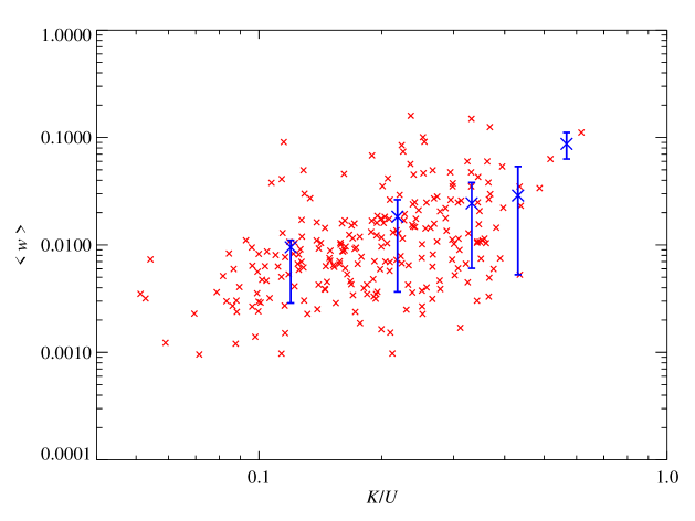
Figure 15 shows the correlation between and . Their correlation coefficient is , which indicates that and are only weakly correlated, making a biased proxy for the dynamical state of a cluster. At any given , the values for scatter by up to two orders of magnitude. This is in agreement with our previous work (\al@2012ApJ…758…74B), where we showed that the correlation between and , the ratio of 3D major to minor axis, is . These two results suggest a reason for the weak correlation of the centroid shift with . This is partially caused by the substantial scatter between the morphological irregularity and asphericity on the one side and dynamical activity of a cluster on the other side, and partially because of projection effects. More work is needed to combine different observationally accessible proxies that correlate more tightly with theoretical measures of dynamical cluster activity, such as the kinetic-to-thermal energy ratio, .
Appendix B Comparing definitions for hydrostatic mass bias
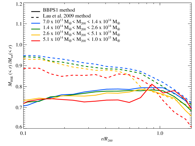
Here we compare various definitions for the bias by hydrostatic equilibrium assumption and review the differing methodologies and definitions used in the (simulation) literature. Direct comparison between our work and others is difficult since the methods used for calculating are different. Previous simulation work used high resolution zoomed simulations of individual clusters (Rasia et al., 2006; Lau et al., 2009; Rasia et al., 2012), where the authors were able to smooth and removed clumps from each cluster before calculating . Other simulations (e.g., Rasia et al., 2006) produced mock X-ray images and performed similar smoothing and clump removal techniques to observations. These cleaning procedures were not preformed in this work (nor in \al@2012ApJ…758…74B, ), because of the different goals of this work. We pursue a theoretically focused approach that should be equally applicable to X-ray (eROSITA) and SZ cluster surveys (by ACT and SPT) and aim at strengthening the understanding of the underlying connection of the hot ICM rather than producing a specific mock observation tailored to a particular observatory.
Another difference is in the definition of . Lau et al. (2009) define the total mass as , which assumes spherical symmetry and a steady state. This is different from our approach (and that in \al@2012ApJ…758…74B, ) since we define . These different definitions for produce significantly different HSE biases, , within as illustrated in Figure 16. Note that the difference of the solid and dashed curves in Figure 16 (at each color and radius) directly measures (since we use the identical in both cases). In particular both approaches yield significantly different radial trends at small radii, presumably due to violation of spherical symmetry and non-stationary, clumpy accretion in the definition of . Adopting the definition of Lau et al. (2009) for the total mass, we recover the same radial trends as these authors, which suggests that the main difference originates from the different definition of rather than .
Appendix C Horizontally sliced SPH kernel integral
To speed up the mass binning of a distribution of SPH particles into a spherical shell, we integrate the mass portion of the SPH-kernel within that shell. We make the approximation that the smoothing length is much smaller than the radius of the shell in question, , so the shell can be thought of as two plane-parallel slices. We obtain a order polynomial fit to the integrated SPH mass fraction below some normalized distance , which is constrained to be exact at :
| (15) | ||||
where for an SPH particle at position . The fit is everywhere accurate to better than of the total mass. Clearly, this approximation breaks down near the center of the cluster (where the shell radius could become comparable to the smoothing length). However, the constraint at guarantees conservation of mass even in the event the approximation breaks down.
Appendix D Variance of projected and for differing number of sector elements
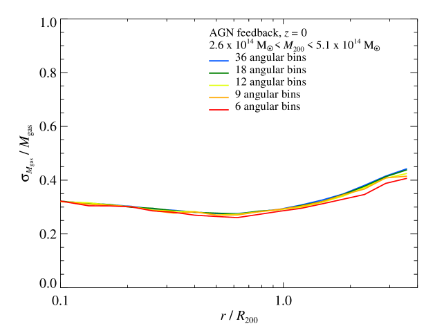
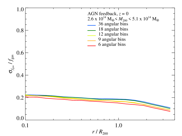
In Figure 17, we address how the 2D angular variances of and change if we vary the number of sector elements. There is almost no difference in for varying number of sector elements and the small systematic decrease in is expected for the increase in bin volume (decrease in sector numbers). Note that this is quite different for the angular variance of the X-ray luminosity, which strongly depends on the number of sector elements, especially in SPH simulations (see Figure 4 of Vazza et al., 2011b). We believe that this increased scatter solely derives from the increased clumping factor with radius (see Figure 1).