Probing CMB Cold Spot through Local Minkowski Functionals

Abstract

Both WMAP and PLANCK missions reported the extremely Cold Spot (CS) centered at Galactic coordinate ($l=209^{\circ}$, $b=-57^{\circ}$) in CMB map. In this paper, we study the local non-Gaussianity of CS by defining the local Minkowski functions. We find that the third Minkowski function $\nu_{2}$ is quite sensitive to the non-Gaussianity caused by CS. Compared with the random Gaussian simulations, WMAP CS deviates from Gaussianity at more than $99\%$ confident level at the scale $R\sim 10^{\circ}$. Meanwhile, we find that cosmic texture provides an excellent explanation for these anomalies related to WMAP CS, which could be further tested by the future polarization data.

I Introduction

Soon after the release of observations of the NASA Wilkinson Microwave Anisotropy Probe (WMAP) satellite on the Cosmic Microwave Background (CMB) temperature and polarization anisotropies, some anomalies in CMB field have also been reported Bennett et al. (2011). Among these, an extremely Cold Spot (CS) centered at Galactic coordinate ($l=209^{\circ}$, $b=-57^{\circ}$) and a characteristic scale about $10^{\circ}$ was detected in the Spherical Mexican Hat Wavelet (SMHW) non-Gaussian analysis (Vielva et al., 2004). Comparing with the distribution derived from the isotropic and Gaussian CMB simulations, due to this CS, the SMHW coefficients of WMAP data have an excess of kurtosis Cruz et al. (2005). The non-Gaussian CS has also been confirmed by using some other statistics Cruz et al. (2007a, 2005); Cayon et al. (2005); Naselsky et al. (2010); Zhang & Huterer (2010); Vielva (2010). At the same time, some analyses on WMAP CS have also been done, such as the non-Gaussian tests for the different detectors and different frequency channels of WMAP satellite Vielva et al. (2004); Cruz et al. (2005), the investigation of the NVSS sources Rudnick et al. (2007); Smith & Huterer (2010), the survey around the CS with MegaCam on the Canada-France-Hawaii Telescope Granett et al. (2009), the redshift survey using VIMOS on VLT towards CS Bremer et al. (2010), and the cross-correlation between WMAP and Faraday depth rotation map Hansen et al. (2012).

Since then, various alternative explanations for this CS have been proposed, including the possible foregrounds Cruz et al. (2006); Hansen et al. (2012), Sunyaev-Zeldovich effect Cruz et al. (2008), the supervoid in the Universe Inoue & Silk (2006, 2007); Inoue (2012), and the cosmic texture Cruz et al. (2007b, 2008). Due to the fact that, nearly all the explanations of CS are related to the local characters of the CMB field, the studies on the local properties of CS are necessary. In the previous work Zhao (2012), we have studied the local non-Gaussian properties of WMAP CS by the local mean temperature, variance, skewness and kurtosis. We found the excesses of the local variance and skewness in the large scales with $R>5^{\circ}$, which implies that WMAP CS is a large-scale non-Gaussian structure, rather than a combination of some small structures. In this paper, we shall focus on the same topic by using the different local statistics. We introduce the local Minkowski Functions (MFs), and apply them to the WMAP data, in particular WMAP CS. Comparing with random Gaussian simulation, we find that for the statistics based on MF $\nu_{2}$, WMAP CS significantly deviates from Gaussianity at large scale, especially at the scale $R\sim 10^{\circ}$. Meanwhile, similar to Zhao (2012), we find that these local non-Gaussianities of WMAP CS can be excellently explained by a cosmic texture. If subtracting this texture from WMAP data, we find that all these anomilies of MFs disappear. So our local analysis of the CS in this paper also strongly supports the cosmic texture explanation.

The outline of this paper is as follows. In Sec. II, we introduce the WMAP data, which will be used in the analysis. In Sec. III, we define the local MFs and apply them into WMAP data. In Section IV, we summarize the main results of this paper.

II The WMAP data

In our analysis, we shall use the WMAP data including the ILC7 map and the NILC5 map. The WMAP instrument is composed of 10 DAs spanning five frequencies from 23 to 94 GHz Bennett et al. (2003). The internal linear combination (ILC) method has been used by WMAP team to generate the ILC maps Hinshaw et al. (2007); Gold et al. (2011). The 7-year ILC (written as “ILC7”) map is a weighted combination from all five original frequency bands, which are smoothed to a common resolution of one degree. For the 5-year WMAP data, in Delabrouille et al. (2009) the authors have made a higher resolution CMB ILC map (written as “NILC5”), an implementation of a constrained linear combination of the channels with minimum error variance on a frame of spherical called needlets note1 . In this paper, we will consider both these two maps for the analysis. Note that these WMAP data have the same resolution parameter $N_{\rm side}=512$, and the corresponding total pixel number $N_{\rm pix}=3145728$.

In comparison with WMAP observations to give constraint on the statistics, a ${\rm\Lambda CDM}$ cosmology is assumed with the cosmological parameters given by the WMAP 7-year best-fit values Komatsu et al. (2011): $100\Omega_{\rm b}h^{2}=2.255$, $\Omega_{c}h^{2}=0.1126$, $\Omega_{\rm\Lambda}=0.725$, $n_{s}=0.968$, $\tau=0.088$ and $\Delta^{2}_{\mathcal{R}}(k_{0})=2.430\times 10^{-9}$ at $k_{0}=0.002{\rm Mpc}^{-1}$. Similar to the previous work (Hansen et al., 2012; Zhao, 2012), to simulate the ILC7 map, we ignore the noises and smooth the simulated map with one degree resolution. And for NILC5, we consider the noise level and beam window function given in Delabrouille et al. (2009). In all the random Gaussian simulations, we assume that the temperature fluctuations and instrument noise follow the Gaussian distribution, and do not consider any effect due to the residual foreground contaminations.

III Applying Local Minkowski Functions to WMAP data

III.1 Minkowski Functions

MFs characterize the morphological properties of convex, compact sets in an $n$-dimensional space. On the 2-dimensional spherical surface $\mathbb{S}^{2}$, any morphological property can be expanded as a linear combination of three MFs, which represent the area, circumference and integrated geodesic curvature of an excursion set Schmalzing & Gorski (1998). For a given threshold $\nu$, it is convenient to define the excursion set $Q_{\nu}$ and its boundary $\partial Q_{\nu}$ of a smooth scalar field $u$ as follows: $Q_{\nu}=\left\{x\in\mathbb{S}^{2}|u(x)>\nu\right\}$ and $\partial Q_{\nu}=\left\{x\in\mathbb{S}^{2}|u(x)=\nu\right\}$. Then, the MFs $v_{0}$, $v_{1}$ and $v_{2}$ can be written as Schmalzing & Gorski (1998),

$$v_{0}(\nu):=\int_{Q_{\nu}}\frac{{\rm d}a}{4\pi},~{}v_{1}:=\int_{\partial Q_{\nu}}\frac{{\rm d}\ell}{16\pi},~{}v_{2}:=\int_{\partial Q_{\nu}}\frac{{\rm d}\ell~{}\kappa}{8\pi^{2}},$$ (1)

where ${\rm d}a$ and ${\rm d}\ell$ denote the surface element of ${\rm\mathbb{S}^{2}}$ and the line element along $\partial{Q_{\nu}}$, respectively. And $\kappa$ is the geodesic curvature. Given a pixelated map with field $u(x_{i})$, these MFs can be numerically calculated by the formulae (Schmalzing & Gorski, 1998; Lim & Simon, 2012)

$$v_{i}(\nu)=\frac{1}{N_{\rm pix}}\sum_{k=1}^{N_{\rm pix}}\mathcal{I}_{i}(\nu,x_{k}),~{}~{}(i=0,1,2),$$ (2)

where

$$\mathcal{I}_{0}(\nu,x_{k}) := \Theta(u-\nu),$$

$$\mathcal{I}_{1}(\nu,x_{k}) := \frac{\delta(u-\nu)}{4}\mathcal{U}_{1}(x_{k}),$$

$$\mathcal{I}_{2}(\nu,x_{k}) := \frac{\delta(u-\nu)}{2\pi}\mathcal{U}_{2}(x_{k}),$$ (3)

$$\mathcal{U}_{1}(x_{k}) := \sqrt{u_{;\theta}^{2}+u_{;\phi}^{2}},$$

$$\mathcal{U}_{2}(x_{k}) := \frac{2u_{;\theta}u_{;\phi}u_{;\theta\phi}-u_{;\theta}^{2}u_{;\phi\phi}-u_{;\phi}^{2}u_{;\theta\theta}}{u_{;\theta}^{2}+u_{;\phi}^{2}}.$$

Note that $u_{;i}$ denotes the covariant differentiation of $u$ with respect to the coordinate $i$. The delta function in these formulae can be numerically approximated through a discretization of threshold space in bins of width $\Delta\nu$ by the stepfunction $\delta_{N}(x)=(\Delta\nu)^{-1}[\Theta(x+\Delta\nu/2)-\Theta(x-\Delta\nu/2)]$. The expectation values of three MFs for a Gaussian random field are also derived in Tomita (1986), which have been explicitly expressed in equations (14) and (15) in Schmalzing & Gorski (1998).

These MFs have been applied by cosmologists to look for derivations from Gaussianity of the perturbations in the CMB Winitzki & Kosowsky (1998); Schmalzing & Gorski (1998); Novikov et al. (1999); Eriksen et al. (2004); Hikage et al. (2006, 2008, 2009); Hikage & Matsubara (2012); Komatsu et al. (2009); Matsubara (2010). In particular, in Lim & Simon (2012) the authors used the MFs to probe the cold/hot disk-like structure in the CMB. However, they found these statistics are noise-dominated for WMAP CS. For a single WMAP or PLANCK resolution map, the method can only detect the highly prominent disk, i.e. extremely cold or hot disk with quite large area. These can be easily understood as follows: since the MFs are constructed on the global sky, the local non-Gaussianity of the cold/hot spot in the relatively small scale has been diluted to be too small.

III.2 Local Minkowski Functions

To study the local properties of WMAP CS, similar to the previous works Bernui & Reboucas (2009, 2010, 2012); Zhao (2012), in this paper we shall define the local MFs as the statistics of CMB field. For a given full-sky WMAP data with $N_{\rm side}=512$ (ILC7 or NILC5), we smooth them using a Gaussian filter with a smoothing scale of $\theta_{s}$. Since MFs are sensitive to the smoothing scale of a density field and thereby we can obtain a variety of information from density fields by using different smoothing levels. In this paper, we focus on both ILC fields smoothed by six different smoothing scales $10^{\prime}$, $20^{\prime}$, $30^{\prime}$, $40^{\prime}$, $50^{\prime}$, $60^{\prime}$. Then, we can construct the corresponding full-sky maps: $\mathcal{U}_{1}(x_{k})$ and $\mathcal{U}_{2}(x_{k})$ defined in Eq. (3), where $u$ is the corresponding ILC temperature anisotropic map.

Now, we can define the local MFs. Let $\Omega(\theta_{j},\phi_{j};R)$ be a spherical cap with aperture of $R$ degree, centered at $(\theta_{j},\phi_{j})$. The local MFs $v_{i}(\nu)$ ($i=0,1,2$) in this cap can be calculated by using Eq. (2), which are denoted as $v_{i}^{j}(\nu;R)$ in the rest of this paper. But here the summation is carried out only for the pixels inside the cap $\Omega(\theta_{j},\phi_{j};R)$. Note that in our calculation, the binning range of threshold $\nu$ is set to be -3.0 to 3.0 with 24 equally spaced bins of $\nu/\sigma$ ($\sigma$ is the standard deviation of $u$-field in this cap) per each MF. In order to quantify the same kind of MFs by a single quantity, following Hikage et al. (2009), for each $i$ (the type of MFs), {$j$, $R$} (the cap) we can define the $\chi^{2}$ as follows:

$$\chi^{2}=\sum_{\alpha\alpha^{\prime}}[v_{i}^{j}(\nu_{\alpha};R)-v_{i}^{\rm th}(\nu_{\alpha};R)]\Sigma_{\alpha\alpha^{\prime}}^{-1}$$

$$\times[v_{i}^{j}(\nu_{\alpha^{\prime}};R)-v_{i}^{\rm th}(\nu_{\alpha^{\prime}};R)],$$ (4)

where $\alpha$ and $\alpha^{\prime}$ denote the binning number of threshold values. $v_{i}^{\rm th}(\nu;R)$ is the theoretical value of $v_{i}^{j}(\nu;R)$, which is independent of the superscript $j$. $\Sigma$ is the corresponding covariance matrix. Although, in principle the theoretical values $v_{i}^{\rm th}(\nu;R)$ for the random Gaussian field can be calculated by the analytical formulae Tomita (1986); Schmalzing & Gorski (1998), there are systematical differences from the numerical results due to the binning of threshold Lim & Simon (2012). In this paper, we avoid this problem by replacing the theoretical value $v_{i}^{\rm th}(\nu;R)$ by the quantity $\langle{v_{i}(\nu;R)}\rangle$, which is the average value of all ${v_{i}^{j}(\nu;R)}$ with $|b_{j}|>30^{\circ}$. And the covariance matrix $\Sigma$ can also be numerically calculated by these quantities ${v_{i}^{j}(\nu;R)}$. Note that the Galactic plane have been excluded to reduce the effect of foreground residuals note2 . Hereafter, we denote this $\chi^{2}$ quantity as $X_{i}^{j}(R)$. Clearly, the values $X_{i}^{j}(R)$ obtained in this way for each cap can be viewed as a measure of non-Gaussianity in the direction of the center of cap $(\theta_{j},\phi_{j})$. For a given aperture $R$, we scan the celestial sphere with evenly distributed spherical caps, and build the $X_{0}(R)$-, $X_{1}(R)$-, $X_{2}(R)$-maps. In our analysis, we have chosen the locations of centroids of spots to be the pixels in $N_{\rm side}=64$ resolution. By choosing different $R$ values, one can study the local properties of CMB field at different scales.

Same to the $V(R)$-map (or $S(R)$-, $K(R)$-maps) defined in Zhao (2012), here we also find that $X_{i}^{j}(R)$ always maximize at the edge of the circles, rather than the center of circles. To overcome this problem and localize the non-Gaussian sources, we define the average quantities

$$\bar{X}_{i}^{j}(R):=\frac{1}{N_{\rm pix}}\sum_{j=1}^{N_{\rm pix}}{X}_{i}^{j}(R),~{}~{}~{}(i=0,1,2),$$ (5)

where $N_{\rm pix}$ is again the pixel number in the $j^{\rm th}$ cap.

We apply the method to the ILC7 data by choosing $R=2^{\circ}$ and $\theta_{s}=60^{\prime}$. The $\bar{X}_{i}$ maps are presented in Fig. 1 (left panels), which clearly show that these local statistics, in particular third MF $v_{2}$, are very sensitive to the foreground residuals and various point sources. The Galactic plane is clearly presented, which is the non-Gaussian area caused by the foreground residuals in ILC7 map. In addition, two important point sources at ($l=209.5^{\circ}$, $b=-20.1^{\circ}$) and ($l=184.9^{\circ}$, $b=-5.98^{\circ}$), as well as several small ones, are also clearly found in the $\bar{X}_{i}$ maps. So we expect these local statistics with small $R$ values can be used to identify the point sources and foreground residuals, which will be discussed in a separate paper. If we choose $R=5^{\circ}$, from the middle panels in Fig. 1 we find the similar results, except for some non-Gaussianities of small point sources, which have been diluted for this larger $R$ case. In the right panels, we have chosen $R=10^{\circ}$, where the significant non-Gaussianity around WMAP CS are clearly presented in all three maps.

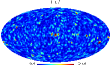
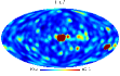
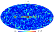
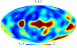
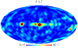
Figure 1: $\bar{X}_{0}(R)$ maps (upper), $\bar{X}_{1}(R)$ maps (middle), and $\bar{X}_{2}(R)$ maps (lower) for ILC7 data with $\theta_{s}=60^{\prime}$ smoothing. In the left panels, we have used $R=2^{\circ}$, in middle panels, $R=5^{\circ}$ is chosen, and in right panel, $R=10^{\circ}$.

Let us turn to NILC5 map, which has the much higher resolution than ILC7. We firstly study effect of different levels of smoothing. By adopting $R=2^{\circ}$, in Fig. 2 we plot the $\bar{X}_{i}$ maps for $\theta_{s}=10^{\prime}$ (left panels) and $\theta_{s}=40^{\prime}$ (right panels). Interesting enough for the lower smoothing case, from the left middle and left lower panels we find the clear structure of ${\rm N}_{\rm obs}$, i.e. the effective observations of WMAP for each pixel. We find a smaller ${\rm N}_{\rm obs}$, which follows a smaller pixel-noise variance, corresponds a larger $\bar{X}_{i}^{j}$. So, these two local MF statistics can also be used to search for the morphology of the pixel-noise variance, which has been hidden in the temperature anisotropy map. We leave this as a future work. Here, in order to reduce the effect of them, we should choose a larger smoothing parameter $\theta_{s}$ as in the right panels in Fig. 2, where we find the morphology of the pixel-noise variance disappears. But the non-Gaussianity in the Galactic place is still there, due to the heavy contamination caused by foreground residuals.

Choosing a common smoothing parameter $\theta_{s}=60^{\prime}$, in Fig. 3 we plot the $\bar{X}_{i}$ maps for $R=2^{\circ}$ (left), $R=5^{\circ}$ (middle) and $R=10^{\circ}$ (right). By comparing with those in Fig. 1, we find that although several non-Gaussian point sources and the foreground residuals in Galactic plane are still there, NILC5 is much cleaner than ILC7, as claimed in Delabrouille et al. (2009). Meanwhile, we find that the non-Gaussianity around WMAP CS are quite significant in the panels with $R=10^{\circ}$, which will be quantified in next subsection.

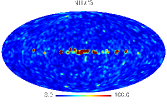
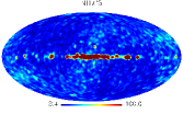
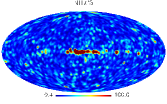
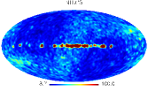
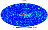
Figure 2: $\bar{X}_{0}(R)$ maps (upper), $\bar{X}_{1}(R)$ maps (middle), and $\bar{X}_{2}(R)$ maps (lower) for NILC5 data with $R=2^{\circ}$. In the left panels, the NILC5 map is smoothed by $\theta_{s}=10^{\prime}$, and in right panels, $\theta_{s}=40^{\prime}$ smoothing is applied.

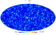
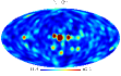
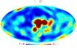
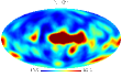
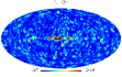
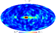
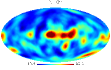
Figure 3: $\bar{X}_{0}(R)$ maps (upper), $\bar{X}_{1}(R)$ maps (middle), and $\bar{X}_{2}(R)$ maps (lower) for NILC5 data with $\theta_{s}=60^{\prime}$ smoothing. In the left panels, we have used $R=2^{\circ}$, in middle panels, $R=5^{\circ}$ is chosen, and in right panel, $R=10^{\circ}$.

III.3 Local Properties of WMAP Cold Spot

Now, let us focus on the local properties of WMAP CS, by comparing with the Gaussian random simulaions. Throughout this section, we only consider the maps which have been smoothed by $\theta_{s}=60^{\prime}$ to exclude the small-scale contaminations.

Firstly, we compare WMAP CS with the spots at the same position ($l=209^{\circ}$, $b=-57^{\circ}$) in the random simulations. For a given $\bar{X}_{i}(R)$ map ($i=0,1,2$) derived from WMAP data, the values of $\bar{X}_{i}(R)$ centered at CS are calculated for the scales of $R=2^{\circ},3^{\circ},4^{\circ},5^{\circ},6^{\circ},7^{\circ},8^{\circ},9^{\circ},10^{\circ},11^{\circ},12^{\circ},13^{\circ},14^{\circ},15^{\circ}$. The statistics for ILC7 maps are displayed in Fig. 4. We compare them with 1000 Gaussian simulations. For each simulated sample, we select the spot at ($l=209^{\circ}$, $b=-57^{\circ}$) and derive the corresponding $\bar{X}_{i}(R)$ maps. Then for each $i$ and $R$, we study the distribution of 1000 $\bar{X}_{i}(R)$ values, and construct the confident intervals for the statistics. The $68\%$, $95\%$ and $99\%$ confident intervals are illustrated in Fig. 4. From this figure, we find that for the $\bar{X}_{0}(R)$ statistics, WMAP CS is consistent with simulations. However, for the $\bar{X}_{1}(R)$ and $\bar{X}_{2}(R)$ statistics with $R>6^{\circ}$, WMAP CS deviates from simulation at more than $99\%$ confident level. For the NILC5 case, we have also obtained the similar results. These show that as anticipated, WMAP CS is not a normal spot. The deviations at large scales imply that WMAP CS seems a nontrivial large-scale structure, rather than a combination of some small non-Gaussian structures (for instance, the point sources or foreground residuals, which always follow the non-Gaussianities in the small scales), which is consistent with the conclusion in Zhao (2012).

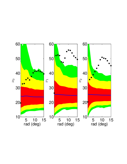
Figure 4: Three statistics for the spots at ($l=209^{\circ}$, $b=-57^{\circ}$). Confidence regions obtained from 1000 Monte Carlo simulations are shown for 68 pre cent (dark central region, red online), 95 pre cent (lighter middle region, yellow online) and 99 pre cent (lightest outer region, green online) levels, as it the mean (solid blue line). The observed statistics for WMAP ILC7 map are shown by the solid dots (black online).

Secondly, we compare WMAP CS with the coldest spots in the Gaussian simulations. For every simulated map with $N_{\rm side}=512$, we search for the coldest spot and derive the corresponding $\bar{X}_{i}(R)$ maps by the same calculations used for WMAP data. Then for each $i$ and $R$, we study the distribution of 1000 $\bar{X}_{i}(R)$ values, and construct the confident intervals for the statistics. The $68\%$, $95\%$ and $99\%$ confident intervals are illustrated in Fig. 5. We find that for the MF $\nu_{0}$, WMAP CS is a normal coldest spot in all the scales when comparing with simulations. For $\nu_{1}$ with $R>7^{\circ}$, WMAP CS deviates from the Gaussianity only at $68\%$ confident level. However, for the MF $\nu_{2}$ with $R>7^{\circ}$, the deviation is quite significant (i.e. more than $95\%$ level). Especially, for $\nu_{2}$ at the scale $R=10^{\circ}\sim 11^{\circ}$, the deviations are more than $99\%$ confident level. And also in the NILC5 case, the similar deviations for these statistics have also been derived. So, we conclude that compared with the coldest spots in simulations, WMAP CS significantly deviates from Gaussianity for MF $\nu_{2}$ at the scale $R\sim 10^{\circ}$. However, in the smaller scales $R<6^{\circ}$, the deviations do not exist. These support that WMAP CS seems a large-scale non-Gaussian structure.

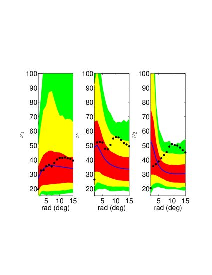
Figure 5: Three statistics for the coldest spots. Confidence regions obtained from 1000 Monte Carlo simulations are shown for 68 pre cent (dark central region, red online), 95 pre cent (lighter middle region, yellow online) and 99 pre cent (lightest outer region, green online) levels, as it the mean (solid blue line). The observed statistics for WMAP ILC7 map are shown by the solid dots (black online).

In Cruz et al. (2007b, 2008), the authors found that the cosmic texture, rather than the other explanations, provides an excellent interpretation for WMAP CS, which has also been strongly supported by studying local mean temperature, variance, skewness and kurtosis in our previous work Zhao (2012). Here we shall test if the local anomalies of WMAP CS found in MFs are consistent with the cosmic texture interpretation. The profile for the CMB temperature fluctuation caused by a collapsing cosmic texture is given by

$$\frac{\Delta T}{T}=-\left\{\begin{array}[]{ll}\frac{\varepsilon}{\sqrt{1+4\left(\frac{\vartheta}{\vartheta_{c}}\right)^{2}}}&\mathrm{if}~{}~{}\vartheta\leq\vartheta_{*}\\ &\\ \frac{\varepsilon}{2}\mathrm{e}^{-\frac{1}{2\vartheta^{2}_{c}}\left(\vartheta^{2}+\vartheta^{2}_{*}\right)}&\mathrm{if}~{}~{}\vartheta>\vartheta_{*}\\ \end{array}\right.$$ (6)

where $\vartheta$ is the angle from the center. $\varepsilon$ is the amplitude parameter, and $\vartheta_{c}$ is the scale parameter. $\vartheta_{*}=\sqrt{3}/2\vartheta_{c}$. By the Bayesian analysis, the best-fit texture parameters were obtained $\varepsilon=7.3\times 10^{-5}$ and $\vartheta_{c}=4.9^{\circ}$ Cruz et al. (2007b). In our calculation, we adopt these best-fit parameters and subtract this cosmic texture structure from the ILC7 and NILC5 maps. Then, we repeat the analyses above by using these subtracted ILC maps. The corresponding results are presented in Fig. 6 for ILC7 and Fig. 7 for NILC5, where we find that WMAP CS becomes quite normal, i.e. it becomes excellently consistent with the normal spots in Gaussian simulations for any MF at any scale. So, we obtain the conclusion: The local analysis of WMAP CS by using the local MF statistics strongly supports the cosmic texture explanation.

Figure 6: Same with Fig. 4, but here the cosmic texture structure has been subtracted from WMAP ILC7 map.

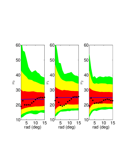
Figure 7: Same with Fig. 6, but here WMAP ILC7 map is replaced by NILC5 map.

IV Conclusion

Since the release of WMAP data, many attentions have been paid to study the non-Gaussian CS at Galactic coordinate ($l=209^{\circ}$, $b=-57^{\circ}$), which might be produced by various small-scale contaminations, such as point sources or foregrounds, the supervoid in the Universe, or some phase transition in the early Universe. In this paper, in order to identify the WMAP CS and discriminate various explanations, we study the local properties of CS by introducing the local MFs as the statistics. We find that compared with random Gaussian simulations, WMAP CS definitely deviates from the normal spots in simulations. In particular, it also deviates from the coldest spots in Gaussian samples at more than $99\%$ confident level at the scale $R\sim 10^{\circ}$. All these support that WMAP CS is a large-scale non-Gaussian structure. Meanwhile, we find that the cosmic texture with a characteristic scale about $10^{\circ}$, which is claimed to the most promising explanation of CS by many authors, can excellently account for these anomalies of the local statistics. So our analysis supports the cosmic texture explanation for WMAP CS.

In the end of this paper, it is important to mention that the non-Gaussianity of WMAP Cold Spot has been confirmed by the recent PLANCK observation Planck Collaboration (2013) on the CMB temperature anisotropies. In the near future, the polarization results of PLANCK mission will be released, which would play a crucial role to test WMAP CS and reveal its physical origin (Cruz et al., 2007b).

Acknowledgements: We appreciate useful discussions with P. Naselsky, J. Kim, M. Hansen and A.M. Frejsel. We acknowledge the use of the Legacy Archive for Microwave Background Data Analysis (LAMBDA). Our data analysis made the use of HEALPix Gorski et al. (2005) and GLESP Doroshkevich et al. (2005). This work is supported by project 973 No.2012CB821804, NSFC No.11173021, 11322324 and project of KIP of CAS.

References

- Bennett et al. (2011) Bennett, C. L. et al., 2011, Astrophys. J. Suppl. Ser. , 192, 17
- Vielva et al. (2004) Vielva, P., Martinez-Gonzalez, E., Barreiro, R. B., Sanz, J. L. & Cayon, L. 2004, Astrophys. J. , 609, 22
- Cruz et al. (2005) Cruz, M., Martinez-Gonzalez, E., Vielva, P. & Cayon, L. 2005, Mon. Not. Roy. Astron. Soc. , 356, 29
- Cruz et al. (2007a) Cruz, M., Cayon, L., Martinez-Gonzalez, E. & Vielva, P. 2007, Astrophys. J. , 655, 11
- Cayon et al. (2005) Cayon, L., Lin, J. & Treaster, A. 2005, Mon. Not. Roy. Astron. Soc. , 362, 826
- Naselsky et al. (2010) Naselsky, P. D., Christensen, P. R., Coles, P., Verkhodanov, O., Novikov, D. & Kim, J. 2010, Astrophys. Bull., 65, 101
- Zhang & Huterer (2010) Zhang, R. & Huterer, D. 2010, Astroparticle Physics, 33, 69
- Vielva (2010) Vielva, P. 2010, arXiv:1008.3051
- Rudnick et al. (2007) Rudnick, L., Brown, S. & Williams, L. R. 2007, Astrophys. J. , 671 40
- Smith & Huterer (2010) Smith, K. M. & Huterer, D. 2010, Mon. Not. Roy. Astron. Soc. , 403, 2
- Granett et al. (2009) Granett, B. R., Szapudi, I. & Neyrinck, M. C. 2009, Astrophys. J. , 714, 825
- Bremer et al. (2010) Bremer, M. N., Silk, J., Davies L. J. M. & Lehnert, M. D. 2010, Mon. Not. Roy. Astron. Soc. , 404, L69
- Hansen et al. (2012) Hansen, M., Zhao, W., Frejsel, A. M., Naselsky, P. D., Kim, J. & Verkhodanov, O. V. 2012, Mon. Not. Roy. Astron. Soc. , 426, 57
- Cruz et al. (2006) Cruz, M., Tucci, M., Martinez-Gonzalez, E. & Vielva, P. 2006, Mon. Not. Roy. Astron. Soc. , 369, 57
- Cruz et al. (2008) Cruz, M., Martinez-Gonzalez, E., Vielva, P., Diego, J. M., Hobson, M. & Turok, N. 2008, Mon. Not. Roy. Astron. Soc. , 390, 913
- Inoue & Silk (2006) Inoue, K. T. & Silk, J. 2006, Astrophys. J. , 648, 23
- Inoue & Silk (2007) Inoue, K. T. & Silk, J. 2006, Astrophys. J. , 664, 650
- Inoue (2012) Inoue, K. T. 2012, Mon. Not. Roy. Astron. Soc. , 421, 2731
- Cruz et al. (2007b) Cruz, M., Turok, N., Vielva, P., Martinez-Gonzalez, E. & Hobson, M. P. 2007, Science, 318, 1612
- Zhao (2012) Zhao, W. 2013, Mon. Not. Roy. Astron. Soc. 433, 3498
- Bennett et al. (2003) Bennett, C. L. et al., 2003, Astrophys. J. Suppl. Ser. , 148, 1
- Hinshaw et al. (2007) Hinshaw, G. et al., 2007, Astrophys. J. Suppl. Ser. , 170, 288
- Gold et al. (2011) Gold, B. et al., 2011, Astrophys. J. Suppl. Ser. , 192, 15
- Delabrouille et al. (2009) Delabrouille, J., Cardoso, J. F., Le Jeune, M., Betoule, M., Fay, G. & Guilloux, F. 2009, A & A, 493, 835
- (25) The similar map for 7-year WMAP data is recently gotten in (Basak & Delabrouille, 2012).
- Basak & Delabrouille (2012) Basak, S. & Delabrouille, J. 2012, Mon. Not. Roy. Astron. Soc. , 419, 1163
- Komatsu et al. (2011) Komatsu, E. et al., 2011, Astrophys. J. Suppl. Ser. , 192, 18
- Schmalzing & Gorski (1998) Schmalzing, J. & Gorski, K. M. 1998, Mon. Not. Roy. Astron. Soc. , 297, 355
- Lim & Simon (2012) Lim, E. A. & Simon, D. 2012, Journal of Cosmology and Astroparticle Physics, 01, 048
- Tomita (1986) Tomita, H. 1986, Progr. Theor. Phys., 76, 952
- Winitzki & Kosowsky (1998) Winitzki, S. & Kosowsky, A. 1998, New Astronomy, 3, 75
- Novikov et al. (1999) Novikov, D. I., Feldman, H. A. & Shandarin, S. F. 1999, International Journal of Modern Physics D, 8, 291
- Eriksen et al. (2004) Eriksen, H. K., Novikov, D. I. & Lilje, P. B. 2004, Astrophys. J. , 612, 64
- Hikage et al. (2006) Hikage, C., Komatsu, E. & Matsubara, T. 2006, Astrophys. J. , 653, 11
- Hikage et al. (2008) Hikage, C., Matsubara, T., Coles, P., Liguori, M., Hansen, F. K. & Matarrese, S. 2008, Mon. Not. Roy. Astron. Soc. , 389, 1439
- Hikage et al. (2009) Hikage, C., Koyama, K., Matsubara, T., Takahashi, T. & Yamaguchi, M. 2009, Mon. Not. Roy. Astron. Soc. , 398, 2188
- Hikage & Matsubara (2012) Hikage, C. & Matsubara, T. 2012, Mon. Not. Roy. Astron. Soc. , 425, 2187
- Komatsu et al. (2009) Komatsu, E. et al., 2009, Astrophys. J. Suppl. Ser. , 180, 330
- Matsubara (2010) Matsubara, T. 2010, Phys. Rev. D, 81, 083505
- Bernui & Reboucas (2009) Bernui, A. & Reboucas, M. J. 2009, Phys. Rev. D, 79, 063528
- Bernui & Reboucas (2010) Bernui, A. & Reboucas, M. J. 2010, Phys. Rev. D, 81, 063533
- Bernui & Reboucas (2012) Bernui, A. & Reboucas, M. J. 2012, Phys. Rev. D, 85, 023522
- (43) Note that, for the WMAP V-band or W-band maps, we always have to apply the complicated masks (such as the KQ75y7 mask) to exclude various contaninations casued by foregrounds and dusts. Thus, there is no way to define the quantity , and the related quantity defined in Eq.(4). This is the reason why we cannot apply the method to the WMAP V-band or W-band maps.
- Planck Collaboration (2013) Planck Coolaboration, arXiv:1303.5083
- Gorski et al. (2005) Gorski, K. M., Hivon, E., Banday, A. J., Wandelt, B. D., Hansen, F. K., Reinecke, M. & Bartelman, M. 2005, Astrophys. J. , 622, 759
- Doroshkevich et al. (2005) Doroshkevich, A. G., Naselsky, P. D., Verkhodanov, O. V., Novikov, D. I., Turchaninov, V. I., Novikov, I. D., Christensen, P. R. & Chiang, L. -Y. 2005, International Journal of Modern Physics D, 14, 275