Physical unitarity for a massive Yang-Mills theory without the Higgs field:
A perturbative treatment

Abstract

In a series of papers, we examine the physical unitarity in a massive Yang-Mills theory without the Higgs field in which the color gauge symmetry is not spontaneously broken and kept intact. For this purpose, we use a new framework proposed in the previous paper Kondo [arXiv:1208.3521] based on a nonperturbative construction of a non-Abelian field describing a massive spin-one vector boson field, which enables us to perform the perturbative and nonperturbative studies on the physical unitarity. In this paper, we present a new perturbative treatment for the physical unitarity after giving the general properties of the massive Yang-Mills theory. Then we reproduce the violation of physical unitarity in a transparent way. This paper is a preliminary work to the subsequent papers in which we present a nonperturbative framework to propose a possible scenario of restoring the physical unitarity in the Curci-Ferrari model.

I Introduction

In the Yang-Mills theory YM54 and quantum chromodynamics (QCD) for strong interactions, both the renormalizability and the physical unitarity are satisfied, as demonstrated first in tHooft71 . Moreover, it is also known that the massive Yang-Mills theory satisfies both the renormalizability and the physical unitarity tHooft71b , if the local gauge invariance is spontaneously broken by the Higgs field Higgs66 and the gauge field acquires the mass through the Higgs mechanism by absorbing the Nambu-Goldstone particle associated with the spontaneous symmetry breakdown. In other words, both the renormalizability and the physical unitarity survive the spontaneous breaking of the gauge symmetry.

It is a long-standing problem DV70 ; SF70 ; Boulware70 ; CF76 ; CF76b ; FMTY81 ; Ojima82 ; BSNW96 ; DTT88 ; RRA04 ; BFQ to clarify whether it is possible or not to construct a massive Yang-Mills model blessed with both the physical unitarity and the renormalizability without the Higgs fields, in which the local gauge symmetry is not spontaneously broken. Here the Lagrangian is assumed to be written in polynomials of the fields (we exclude the nonpolynomial type FMTY81 from our discussions). We are anxious to find such a model for understanding the mass gap and confinement caused by the strong interactions Cornwall82 ; decoupling ; decoupling-lattice ; TW11 ; scaling , since the Higgs field does not exist and the color gauge symmetry is kept intact in QCD. Indeed, there are continued attempts to look for an alternative way to describe massive non-Abelian gauge fields without the Higgs field DV70 ; SF70 ; Boulware70 ; CF76 ; CF76b ; FMTY81 ; Ojima82 ; BSNW96 ; DTT88 ; RRA04 . However, all these efforts were unsuccessful in coping with both renormalizability and unitarity very well: In all the models proposed so far for the massive Yang-Mills theory without the Higgs fields, it seems that the renormalizability and the physical unitarity are not compatible with each other, although there are some models which satisfy either the renormalizability or the physical unitarity. See DTT88 ; RRA04 for reviews and BFQ for later developments.

For this purpose, we start once again from the Curci-Ferrari (CF) model CF76 , which is a massive extension of the massless Yang-Mills theory in the most general renormalizable gauge having both the Becchi-Rouet-Stora-Tyutin (BRST) and anti-BRST symmetries Baulieu85 . In preceding studies for the CF model CF76 ; CF76b ; Ojima82 ; BSNW96 , the CF model is proved to be renormalizable, whereas the CF model has been concluded to violate physical unitary CF76b ; Ojima82 ; BSNW96 . However, the preceding studies are restricted to considerations in the perturbation theory. We need a nonperturbative framework to draw a definite conclusion to this issue.

In a previous paper Kondo12 , therefore, we have presented a nonperturbative construction of a massive Yang-Mills field $\mathscr{K}_{\mu}$ which describes a non-Abelian massive spin-one vector boson with the correct physical degrees of freedom without the Higgs field Higgs66 . This is achieved by finding a nonlinear but local transformation from the original fields in the CF model to the physical massive vector field $\mathscr{K}_{\mu}$ which is invariant under the modified BRST and anti-BRST transformation. As an application, we have written down a local mass term for the Yang-Mills field and a dimension-two condensate, which are exactly invariant under the modified BRST transformation, Lorentz transformation and color rotation. The resulting massive Yang-Mills model is regarded as a low-energy effective theory of QCD, which enables us to understand the decoupling solution decoupling characterizing the deep infrared regime responsible for color confinement KO79 ; Gribov78 .

In a series of papers, we give the perturbative and nonperturbative studies on the physical unitarity Kondo12a in the massive Yang-Mills theory constructed in the previous paper Kondo12 . In the ordinary massless Yang-Mills theory, the physical unitarity is a first step of understanding color confinement KO79 : In the intermediate state, the contributions from the unphysical gauge modes, i.e., the longitudinal and scalar modes are exactly canceled by those of the ghost and antighost, which is a special case of the quartet mechanism KO78 . We clarify how the situation changes in the massive case. Moreover, we clarify the reason for failures of the preceding attempts from our viewpoint.

This paper is the first of the planned papers for discussing the perturbative and nonperturbative physical unitarity in the massive Yang-Mills theory without the Higgs field. In this paper we present a new perturbative treatment for the physical unitarity after reviewing the general properties of the massive Yang-Mills theory. Then we reproduce the violation of physical unitarity in a transparent way. In subsequent papers, we present a nonperturbative framework to discuss a possible scenario of restoring the physical unitarity in the massive Yang-Mills theory.

Finally, we mention the difference between the unitarity and physical unitarity of the scattering matrix from our point of view. For the tree-level scattering amplitude between two longitudinally polarized vector bosons, it is known PS95 ; CLT73 ; LQT77 that the scattering probability as a function of the energy $E$ becomes greater than 1 above a critical value $E_{c}$, since the amplitude grows with the energy $E$ like $g^{2}E^{2}/M^{2}$ where $M$ is the mass of the vector boson and $g$ is the coupling constant for the self-interactions among vector bosons. This implies that the perturbative unitarity breaks down in high-energy $E\geq E_{c}$. Therefore, for the perturbative unitarity to be satisfied, the energy must be restricted to low-energy $E<E_{c}$, which is called the unitarity bound. (The violation of the unitarity condition for the scattering amplitude in high energy is understood from the Nambu-Goldstone equivalence theorem CLT73 and the low-energy theorem.) In the Higgs sector of weak interactions in the standard model, the Higgs particle exists and the exchange of the Higgs particle affects the amplitude so that the amplitude approaches a constant at energies far above the Higgs pole. Consequently, the Higgs mass must be less than an upper bound. If such new physical degrees of freedom do not exist, this behavior is not modified and the unitarity violation in high energy cannot be avoided in the massive Yang-Mills theory, since the Nakanishi-Lautrup (NL) auxiliary field can be integrated out and the ghosts can play no role in the tree-level amplitude. In our works, we regard the CF model as a low-energy effective theory of the Yang-Mills theory to be valid in the region $E<E_{c}$ for discussing color confinement. We restrict our examination on the physical unitarity to a sufficiently low-energy region below a few GeV to evade the unitarity violation and consider only the physical unitarity, i.e., unphysical mode cancellation in our papers. Therefore, the well-known fact about the unitarity violation in the above does not contradict our research on the physical unitarity.

This paper is organized as follows.

In section II, we introduce a massive Yang-Mills theory without the Higgs field and define the CF model as a special case. The CF model is not invariant under the usual BRST and anti-BRST transformations. However, the CF model can be made invariant by modifying the BRST and anti-BRST transformations. The cost of introducing the mass term is the violation of nilpotency of the modified BRST and anti-BRST transformations. We point out an important fact that even the modified BRST (anti-BRST)-invariant quantity depends on a parameter $\beta$ in the $M\not=0$ case. This should be compared with the $M=0$ case, in which $\beta$ is a gauge-fixing parameter and the BRST-invariant quantity does not depend on $\beta$, which means that the physics does not depend on $\beta$ in the $M=0$ case. This is not the case for $M\not=0$.

In section III, we summarize the result obtained in the previous paper Kondo12 on a nonperturbative construction of a non-Abelian massive Yang-Mills field $\mathscr{K}_{\mu}$ under the requirements which guarantee (i) the modified BRST (and anti-BRST) invariance, (ii) correct degrees of freedom for describing a massive spin-one particle, and (iii) the expected transformation rule under color rotation. We write down the massive vector field explicitly in terms of the original Yang-Mills field, the Faddeev-Popov (FP) ghost field, antighost field and the NL field in the CF model.

In section IV, we give a perturbative framework of the CF model in terms of the new field variable $\mathscr{K}_{\mu}$. We give the Feynman rules up to the order $g$.

In section V, we check the physical unitarity in the massless Yang-Mills theory. Using a simple example, it is demonstrated in the lowest order of perturbation theory that the physical unitarity follows from the cancellation among unphysical modes: the longitudinal and scalar modes of the Yang-Mills field together with the FP ghost and antighost.

In section VI, we review a conventional argument for the violation of physical unitarity in the massive Yang-Mills theory without the Higgs field. Using a simple example corresponding to the previous section, we show that the violation of physical unitarity follows from the incomplete cancellation among unphysical modes: the scalar mode with the FP ghost and antighost.

In section VII, we begin with a new analysis on the physical unitarity of the CF model based on a novel framework using the field $\mathscr{K}_{\mu}$ given in section III. In this section, we give a new perturbative analysis using the result of section V. We confirm that the physical unitarity is indeed violated in the CF model in the framework of the perturbation theory in the coupling constant. It is easily seen that the violation of physical unitarity follows from the incomplete cancellation among unphysical modes: the NL field (corresponding to the scalar mode) with the FP ghost and antighost. We discuss how to avoid the violation of physical unitarity within the perturbative framework.

In the final section, we summarize the results and mention the perspective on the next work.

In Appendix A, we calculate the Jacobian associated with the change of variables from the original CF model to the new theory written in terms of new variables. In Appendix B, the Feynman rules are given up to the next order $g^{2}$, with which we supplement the results of section V.

II The Curci-Ferrari model and the modified BRST transformation

In order to look for a candidate of the massive Yang-Mills theory without the Higgs field, we start from the usual massless Yang-Mills theory in the most general Lorentz gauge formulated in a manifestly Lorentz covariant way. The total Lagrangian density is written in terms of the Yang-Mills field $\mathscr{A}_{\mu}$, the FP ghost field $\mathscr{C}$, the antighost field $\bar{\mathscr{C}}$ and the NL field $\mathscr{N}$. As a candidate of the massive Yang-Mills theory without the Higgs field, we add the “mass term” $\mathscr{L}_{m}$:

$$\mathscr{L}^{\rm{tot}}_{m\rm{YM}}= \mathscr{L}_{\rm{YM}}+\mathscr{L}_{\rm{GF+FP}}+\mathscr{L}_{m},$$ (1a)

$$\mathscr{L}_{\rm{YM}}= -\frac{1}{4}\mathscr{F}_{\mu\nu}\cdot\mathscr{F}^{\mu\nu},$$ (1b)

$$\mathscr{L}_{\rm{GF+FP}}= \frac{\alpha}{2}\mathscr{N}\cdot\mathscr{N}+\frac{\beta}{2}\mathscr{N}\cdot\mathscr{N}$$

$$+\mathscr{N}\cdot\partial^{\mu}\mathscr{A}_{\mu}-\frac{\beta}{2}g\mathscr{N}\cdot(i\bar{\mathscr{C}}\times\mathscr{C})$$

$$+i\bar{\mathscr{C}}\cdot\partial^{\mu}\mathscr{D}_{\mu}[\mathscr{A}]\mathscr{C}$$

$$+\frac{\beta}{4}g^{2}(i\bar{\mathscr{C}}\times\mathscr{C})\cdot(i\bar{\mathscr{C}}\times\mathscr{C})$$

$$= \mathscr{N}\cdot\partial^{\mu}\mathscr{A}_{\mu}+i\bar{\mathscr{C}}\cdot\partial^{\mu}\mathscr{D}_{\mu}[\mathscr{A}]\mathscr{C}$$

$$+\frac{\beta}{4}(\bar{\mathscr{N}}\cdot\bar{\mathscr{N}}+\mathscr{N}\cdot\mathscr{N})+\frac{\alpha}{2}\mathscr{N}\cdot\mathscr{N},$$ (1c)

$$\mathscr{L}_{m}= \frac{1}{2}M^{2}\mathscr{A}_{\mu}\cdot\mathscr{A}^{\mu}+\beta M^{2}i\bar{\mathscr{C}}\cdot\mathscr{C},$$ (1d)

where $\alpha$ and $\beta$ are parameters corresponding to the gauge-fixing parameters in the $M\rightarrow 0$ limit, $\mathscr{D}_{\mu}[\mathscr{A}]\mathscr{C}(x):=\partial_{\mu}\mathscr{C}(x)+g\mathscr{A}(x)\times\mathscr{C}(x)$, and

$$\bar{\mathscr{N}}:=-\mathscr{N}+gi\bar{\mathscr{C}}\times\mathscr{C}.$$ (2)

The $\alpha=0$ case is the CF model with the coupling constant $g$, the mass parameter $M$ and the parameter $\beta$. In the Abelian limit with vanishing structure constants $f^{ABC}=0$, the FP ghosts decouple and the CF model reduces to the Nakanishi model Nakanishi72 .

In what follows, we restrict our considerations to the $\alpha=0$ case. In the $\alpha=0$ case, $\mathscr{L}_{\rm YM}+\mathscr{L}_{\rm GF+FP}$ is constructed so as to be invariant under both the usual BRST transformation:

$$\begin{cases}{\bm{\delta}}\mathscr{A}_{\mu}(x)=\mathscr{D}_{\mu}[\mathscr{A}]\mathscr{C}(x)\\ {\bm{\delta}}\mathscr{C}(x)=-\frac{g}{2}\mathscr{C}(x)\times\mathscr{C}(x)\\ {\bm{\delta}}\bar{\mathscr{C}}(x)=i\mathscr{N}(x)\\ {\bm{\delta}}\mathscr{N}(x)=0\\ \end{cases},$$ (3)

and anti-BRST transformation:

$$\begin{cases}\bar{\bm{\delta}}\mathscr{A}_{\mu}(x)=\mathscr{D}_{\mu}[\mathscr{A}]\bar{\mathscr{C}}(x)\\ \bar{\bm{\delta}}\bar{\mathscr{C}}(x)=-\frac{g}{2}\bar{\mathscr{C}}(x)\times\bar{\mathscr{C}}(x)\\ \bar{\bm{\delta}}\mathscr{C}(x)=i\bar{\mathscr{N}}(x)\\ \bar{\bm{\delta}}\bar{\mathscr{N}}(x)=0\end{cases}.$$ (4)

Indeed, it is checked that

$${\bm{\delta}}\mathscr{L}_{\rm{YM}}=0,\quad{\bm{\delta}}\mathscr{L}_{\rm{GF+FP}}=0,$$ (5)

$$\bar{\bm{\delta}}\mathscr{L}_{\rm{YM}}=0,\quad\bar{\bm{\delta}}\mathscr{L}_{\rm{GF+FP}}=0.$$ (6)

This is not the case for the mass term $\mathscr{L}_{m}$, i.e.,

$${\bm{\delta}}\mathscr{L}_{m}\neq 0.$$ (7)

Even in the presence of the mass term $\mathscr{L}_{m}$, however, the total Lagrangian $\mathscr{L}_{\rm mYM}^{\rm tot}$ can be made invariant by modifying the BRST transformation CF76 : $\delta_{\rm BRST}^{\prime}=\lambda{\bm{\delta}}^{\prime}$ with a Grassmannian number $\lambda$ and

$$\begin{cases}{\bm{\delta}}^{\prime}\mathscr{A}_{\mu}(x)=\mathscr{D}_{\mu}[\mathscr{A}]\mathscr{C}(x)\\ {\bm{\delta}}^{\prime}\mathscr{C}(x)=-\frac{g}{2}\mathscr{C}(x)\times\mathscr{C}(x)\\ {\bm{\delta}}^{\prime}\bar{\mathscr{C}}(x)=i\mathscr{N}(x)\\ {\bm{\delta}}^{\prime}\mathscr{N}(x)=M^{2}\mathscr{C}(x)\end{cases}.$$ (8)

The modified BRST transformation deforms the BRST transformation of the NL field and reduces to the usual BRST transformation in the limit $M\rightarrow 0$. It should be remarked that ${\bm{\delta}}^{\prime}\mathscr{L}^{\rm tot}_{\rm mYM}=0$ follows from

$$0={\bm{\delta}}^{\prime}(\mathscr{L}_{\rm GF+FP}+\mathscr{L}_{m}),$$ (9)

while

$${\bm{\delta}}^{\prime}\mathscr{L}_{m}\neq 0,\quad{\bm{\delta}}^{\prime}\mathscr{L}_{\rm GF+FP}\neq 0.$$ (10)

Similarly, the total action is invariant under a modified anti-BRST transformation $\bar{{\bm{\delta}}}^{\prime}$ defined by

$$\begin{cases}\bar{\bm{\delta}}^{\prime}\mathscr{A}_{\mu}(x)=\mathscr{D}_{\mu}[\mathscr{A}]\bar{\mathscr{C}}(x)\\ \bar{\bm{\delta}}^{\prime}\bar{\mathscr{C}}(x)=-\frac{g}{2}\bar{\mathscr{C}}(x)\times\bar{\mathscr{C}}(x)\\ \bar{\bm{\delta}}^{\prime}\mathscr{C}(x)=i\bar{\mathscr{N}}(x)\\ \bar{\bm{\delta}}^{\prime}\bar{\mathscr{N}}(x)=-M^{2}\bar{\mathscr{C}}(x)\end{cases},$$ (11)

which reduces to the usual anti-BRST transformation in the limit $M\to 0$. It is sometimes useful to give another form:

$${\bm{\delta}}^{\prime}\mathscr{\bar{N}}(x)= g\mathscr{\bar{N}}(x)\times\mathscr{C}(x)-M^{2}\mathscr{C}(x),$$

$$\bar{{\bm{\delta}}}^{\prime}\mathscr{N}(x)= g\mathscr{N}(x)\times\bar{\mathscr{C}}(x)+M^{2}\bar{\mathscr{C}}(x).$$ (12)

Moreover, the path-integral integration measure $\mathcal{D}\mathscr{A}\mathcal{D}\mathscr{C}\mathcal{D}\bar{\mathscr{C}}\mathcal{D}\mathscr{N}$ is invariant under the modified BRST transformation. Indeed, it has been shown in Kondo12 that the Jacobian associated to the change of integration variables $\Phi(x)\to\Phi^{\prime}(x)=\Phi(x)+\lambda{\bm{\delta}}^{\prime}\Phi(x)$ for the integration measure is equal to one.

However, the modified BRST transformation violates the nilpotency when $M\not=0$:

$$\begin{cases}{\bm{\delta}}^{\prime}{\bm{\delta}}^{\prime}\mathscr{A}_{\mu}(x)=0,\\ {\bm{\delta}}^{\prime}{\bm{\delta}}^{\prime}\mathscr{C}(x)=0,\\ {\bm{\delta}}^{\prime}{\bm{\delta}}^{\prime}\bar{\mathscr{C}}(x)=i{\bm{\delta}}^{\prime}\mathscr{N}(x)=iM^{2}\mathscr{C}(x)\neq 0,\\ {\bm{\delta}}^{\prime}{\bm{\delta}}^{\prime}\mathscr{N}(x)=M^{2}{\bm{\delta}}^{\prime}\mathscr{C}(x)=-M^{2}\frac{g}{2}\mathscr{C}(x)\times\mathscr{C}(x)\neq 0.\end{cases}$$ (13)

The nilpotency is violated also for the modified anti-BRST transformation when $M\not=0$:

$$\begin{cases}\bar{{\bm{\delta}}}^{\prime}\bar{{\bm{\delta}}}^{\prime}\mathscr{A}_{\mu}(x)=0,\\ \bar{{\bm{\delta}}}^{\prime}\bar{{\bm{\delta}}}^{\prime}\bar{\mathscr{C}}(x)=0,\\ \bar{{\bm{\delta}}}^{\prime}\bar{{\bm{\delta}}}^{\prime}\mathscr{C}(x)=i\bar{{\bm{\delta}}}^{\prime}\bar{\mathscr{N}}(x)=-iM^{2}\bar{\mathscr{C}}(x)\neq 0,\\ \bar{{\bm{\delta}}}^{\prime}\bar{{\bm{\delta}}}^{\prime}\bar{\mathscr{N}}(x)=-M^{2}\bar{{\bm{\delta}}}^{\prime}\bar{\mathscr{C}}(x)=M^{2}\frac{g}{2}\bar{\mathscr{C}}(x)\times\bar{\mathscr{C}}(x)\neq 0.\end{cases}$$ (14)

In the limit $M\to 0$, the modified BRST and anti-BRST transformations reduce to the usual BRST and anti-BRST transformations and become nilpotent.

Moreover, it is checked that the modified BRST and modified anti-BRST transformations no longer anticommute in the $M\not=0$ case:

$$\begin{cases}\{{\bm{\delta}}^{\prime},\bar{\bm{\delta}}^{\prime}\}\mathscr{A}_{\mu}(x)=0,\\ \{{\bm{\delta}}^{\prime},\bar{\bm{\delta}}^{\prime}\}\mathscr{C}(x)=-iM^{2}\mathscr{C}(x),\\ \{{\bm{\delta}}^{\prime},\bar{\bm{\delta}}^{\prime}\}\bar{\mathscr{C}}(x)=iM^{2}\mathscr{\bar{C}}(x),\\ \{{\bm{\delta}}^{\prime},\bar{\bm{\delta}}^{\prime}\}\mathscr{N}(x)=0.\end{cases}$$ (15)

In the limit $M\to 0$, the anticommutativity is recovered, $\{{\bm{\delta}}^{\prime},\bar{\bm{\delta}}^{\prime}\}\to 0$.

Let $W$ be the generating functional of the connected Green functions defined from the vacuum functional $Z[J]$ with the source $J$ for an operator $\mathscr{O}$ as a functional of $\Phi$:

$$e^{iW[J]}:=Z[J] :=\int\mathcal{D}\mathscr{A}\mathcal{D}\mathscr{C}\mathcal{D}\bar{\mathscr{C}}\mathcal{D}\mathscr{N}$$

$$\times\exp\left\{iS^{\rm tot}_{m\rm{YM}}+i\int d^{D}xJ(x)\cdot\mathscr{O}(x)\right\}.$$ (16)

Then the derivative of $W$ with respect to $\beta$ is given by

$$\frac{\partial W[J]}{\partial\beta}=\frac{1}{i}\frac{\partial\ln Z[J]}{\partial\beta}=\frac{1}{i}Z[J]^{-1}\frac{\partial Z[J]}{\partial\beta}=\Big{\langle}\frac{\partial S^{\rm tot}_{m\rm{YM}}}{\partial\beta}\Big{\rangle}_{J},$$ (17)

where

$$\frac{\partial S^{\rm tot}_{m\rm{YM}}}{\partial\beta}=\int d^{D}x\left[i{\bm{\delta}}^{\prime}\bar{{\bm{\delta}}}^{\prime}\left(\frac{1}{2}i\bar{\mathscr{C}}\cdot\mathscr{C}\right)+\frac{1}{2}M^{2}i\bar{\mathscr{C}}\cdot\mathscr{C}\right].$$ (18)

This follows from the fact that $\mathscr{L}_{\rm GF+FP}+\mathscr{L}_{m}$ is written as Kondo12

$$\mathscr{L}_{\rm GF+FP}+\mathscr{L}_{m}= i{\bm{\delta}}^{\prime}\bar{{\bm{\delta}}}^{\prime}\left(\frac{1}{2}\mathscr{A}^{\mu}\cdot\mathscr{A}_{\mu}+\frac{\beta}{2}i\bar{\mathscr{C}}\cdot\mathscr{C}\right)$$

$$+\frac{\beta}{2}M^{2}i\bar{\mathscr{C}}\cdot\mathscr{C}+\frac{1}{2}M^{2}\mathscr{A}_{\mu}\cdot\mathscr{A}^{\mu}.$$ (19)

If we require the modified BRST invariance of the vacuum:

$$Q_{\rm BRST}^{\prime}|0\rangle=0,$$ (20)

we find the $\beta$ dependence of $W[J]$:

$$\frac{\partial W[J]}{\partial\beta}=\int d^{D}x\frac{1}{2}M^{2}\langle i\bar{\mathscr{C}}(x)\cdot\mathscr{C}(x)\rangle_{J}\not=0.$$ (21)

Therefore, for $M\not=0$, $W[J]$ depends on the parameter $\beta$. This result should be compared with the $M=0$ case, in which $\beta$ is a gauge fixing parameter and hence $W[J]$ should not depend on $\beta$. In the $M=0$ case, any choice of $\beta$ gives the same $W[J]$. However, this is not the case for $M\not=0$. The $\beta$ dependence of the CF model was pointed out also in Lavrov12 using different arguments.

III Defining a massive Yang-Mills field

We require the following properties to construct a non-Abelian massive spin-one vector boson field $\mathscr{K}_{\mu}(x)$ in a nonperturbative way:

1. $\mathscr{K}_{\mu}$ has the modified BRST invariance (off mass shell):

   $${\bm{\delta}}^{\prime}\mathscr{K}_{\mu}=0.$$ (22)

2. $\mathscr{K}_{\mu}$ is divergenceless (on mass shell):

   $$\partial^{\mu}\mathscr{K}_{\mu}=0.$$ (23)

3. $\mathscr{K}_{\mu}$ obeys the adjoint transformation under the color rotation:

   $$\mathscr{K}_{\mu}(x)\to U\mathscr{K}_{\mu}(x)U^{-1},\quad U=\exp[i\varepsilon^{A}Q^{A}],$$ (24)

which has the infinitesimal version:

$$\delta\mathscr{K}_{\mu}(x)=\varepsilon\times\mathscr{K}_{\mu}(x).$$ (25)

The field $\mathscr{K}_{\mu}$ is identified with the non-Abelian version of the physical massive vector field with spin one, as ensured by the above properties. Here (i) guarantees that $\mathscr{K}_{\mu}$ belong to the physical field creating a physical state with positive norm. (ii) guarantees that $\mathscr{K}_{\mu}$ have the correct degrees of freedom as a massive spin-one particle, i.e., three in the four-dimensional spacetime, i.e., two transverse and one longitudinal modes, excluding one scalar mode. (iii) guarantees that $\mathscr{K}_{\mu}$ obey the same transformation rule as that of the original gauge field $\mathscr{A}_{\mu}$

We observe that the total Lagrangian of the CF model is invariant under the (infinitesimal) global gauge transformation or color rotation defined by

$$\delta\Phi(x):=[\varepsilon^{C}iQ^{C},\Phi(x)]=\varepsilon\times\Phi(x),$$

$$\quad{\rm for}\quad\Phi=\mathscr{A}_{\mu},\mathscr{N},\mathscr{C},\bar{\mathscr{C}},$$ (26)

$$\delta\varphi(x):=[\varepsilon^{C}iQ^{C},\varphi(x)]=-i\varepsilon\varphi(x),$$ (27)

where $\varphi$ is a matter field, which is also written as

$$\delta\Phi^{A}(x)=f^{ABC}\varepsilon^{B}\Phi^{C}(x),$$

$$\delta\varphi_{a}(x)=-i\varepsilon^{A}(T^{A})_{a}^{\ b}\varphi_{b}(x)=-i\varepsilon^{A}(T^{A}\varphi)_{a},$$ (28)

where the conserved Noether charge $Q^{A}:=\int d^{3}x\mathscr{J}^{0,A}_{\rm color}$ obtained from the color current $\mathscr{J}^{0}_{\rm color}$ is called the color charge and is equal to the generator of the color rotation.

It has been shown Kondo12 that such a field $\mathscr{K}_{\mu}$ is obtained by a nonlinear but local transformation from the original fields $\mathscr{A}_{\mu}$, $\mathscr{C}$, $\bar{\mathscr{C}}$ and $\mathscr{N}$ of the CF model:

$$\mathscr{K}_{\mu}:= \mathscr{A}_{\mu}-M^{-2}\partial_{\mu}\mathscr{N}-gM^{-2}\mathscr{A}_{\mu}\times\mathscr{N}$$

$$+gM^{-2}\partial_{\mu}\mathscr{C}\times i\bar{\mathscr{C}}+g^{2}M^{-2}(\mathscr{A}_{\mu}\times\mathscr{C})\times i\bar{\mathscr{C}}.$$ (29)

In the Abelian limit or the lowest order of the coupling constant $g$, $\mathscr{K}_{\mu}$ reduces to the Proca field for massive vector:

$$\mathscr{K}_{\mu}\to\mathscr{A}_{\mu}-\frac{1}{M^{2}}\partial_{\mu}\mathscr{N}:=U_{\mu}.$$ (30)

It should be remarked that $U_{\mu}$ is invariant under the Abelian version of the modified BRST, but it is not invariant under the non-Abelian modified BRST transformation.

The new field $\mathscr{K}_{\mu}$ is converted to a simple form:

$$\mathscr{K}_{\mu}(x)=\mathscr{A}_{\mu}(x)+\frac{1}{M^{2}}i{\bm{\delta}}^{\prime}\bar{{\bm{\delta}}}^{\prime}\mathscr{A}_{\mu}(x).$$ (31)

It has been explicitly shown in Kondo12 that the field $\mathscr{K}_{\mu}$ defined by (29) or (31) satisfies all the above properties. The field $\mathscr{K}_{\mu}$ plays the role of the non-Abelian massive vector field and is identified with a non-Abelian version of the spin-one massive vector field. Equation (29) gives a transformation from $\mathscr{A}_{\mu},\mathscr{N},\mathscr{C}$ and $\bar{\mathscr{C}}$ to $\mathscr{K}_{\mu}$.

As an immediate application of the above result, we can construct a mass term which is invariant simultaneously under the modified BRST transformation, Lorentz transformation and color rotation:

$$\frac{1}{2}M^{2}\mathscr{K}_{\mu}(x)\cdot\mathscr{K}^{\mu}(x).$$ (32)

This can be useful as a regularization scheme for avoiding infrared divergences in non-Abelian gauge theories. Moreover, we can obtain a dimension-two condensate which is modified BRST invariant, Lorentz invariant, and color-singlet:

$$\langle\mathscr{K}_{\mu}(x)\cdot\mathscr{K}^{\mu}(x)\rangle.$$ (33)

This dimension-two condensate is off-shell (modified) BRST invariant and should be compared with the dimension-two condensate proposed in Kondo01 ; KMSI02 :

$$\Big{\langle}\frac{1}{2}\mathscr{A}_{\mu}(x)\cdot\mathscr{A}^{\mu}(x)+\beta\mathscr{C}(x)\cdot\mathscr{\bar{C}}(x)\Big{\rangle},$$ (34)

which is only on-shell BRST invariant.

The original CF Lagrangian $\mathscr{L}_{\rm mYM}^{\rm tot}[\mathscr{A}_{\mu},\mathscr{C},\bar{\mathscr{C}},\mathscr{N}]$ is written in terms of $\mathscr{A}_{\mu},\mathscr{C},\bar{\mathscr{C}}$ and $\mathscr{N}$. The new theory is specified by $\mathscr{L}_{\rm mYM}^{\rm tot}[\mathscr{K}_{\mu},\mathscr{C},\bar{\mathscr{C}},\mathscr{N}]$ written in terms of $\mathscr{K}_{\mu},\mathscr{C},\bar{\mathscr{C}}$ and $\mathscr{N}$ with the symmetry:

$$\begin{cases}{\bm{\delta}}^{\prime}\mathscr{K}_{\mu}(x)=0\\ {\bm{\delta}}^{\prime}\mathscr{C}(x)=-\frac{g}{2}\mathscr{C}(x)\times\mathscr{C}(x)\\ {\bm{\delta}}^{\prime}\bar{\mathscr{C}}(x)=i\mathscr{N}(x)\\ {\bm{\delta}}^{\prime}\mathscr{N}(x)=M^{2}\mathscr{C}(x)\end{cases}.$$ (35)

IV Perturbative framework of the massive Yang-Mills theory

Equation (29) gives a transformation from $\mathscr{A}_{\mu},\mathscr{C},\bar{\mathscr{C}}$ and $\mathscr{N}$ to $\mathscr{K}_{\mu}$. In order to write explicitly the non-Abelian massive Yang-Mills theory without the Higgs field, we rewrite the original Lagrangian written in terms of $\mathscr{A}_{\mu},\mathscr{N},\mathscr{C}$ and $\bar{\mathscr{C}}$ into the new Lagrangian written in terms of $\mathscr{K}_{\mu},\mathscr{N},\mathscr{C}$ and $\bar{\mathscr{C}}$. For this purpose, we need the inverse transformation of (29), namely $\mathscr{A}_{\mu}$ as a function of $\mathscr{K}_{\mu},\mathscr{N},\mathscr{C}$ and $\bar{\mathscr{C}}$. But the inverse transformation cannot be given in a closed form, since (29) is a nonlinear transformation. In order to perform the perturbative calculation, it is sufficient to know the order by order expression of the inverse transformation. By using (29) in the form:

$$\mathscr{A}_{\mu}= \mathscr{K}_{\mu}+M^{-2}\partial_{\mu}\mathscr{N}+gM^{-2}\mathscr{A}_{\mu}\times\mathscr{N}$$

$$-gM^{-2}\partial_{\mu}\mathscr{C}\times i\bar{\mathscr{C}}-g^{2}M^{-2}(\mathscr{A}_{\mu}\times\mathscr{C})\times i\bar{\mathscr{C}},$$ (36)

we find that the right-hand side contains the order $g^{0},g^{1}$ and $g^{2}$ terms. By iterative procedures, we obtain

$$\mathscr{A}_{\mu}= \mathscr{K}_{\mu}+M^{-2}\partial_{\mu}\mathscr{N}-gM^{-2}i\bar{\mathscr{C}}\times\partial_{\mu}\mathscr{C}$$

$$+gM^{-2}\mathscr{K}_{\mu}\times\mathscr{N}+gM^{-4}\partial_{\mu}\mathscr{N}\times\mathscr{N}+O(g^{2}).$$ (37)

The propagator of $\mathscr{K}_{\mu}$ is obtained from the order $g^{0}$ terms, i.e., $\mathscr{A}_{\mu}=\mathscr{K}_{\mu}+\frac{1}{M^{2}}\partial_{\mu}\mathscr{N}$, as in the Abelian case, and hence the propagator is not modified from the Proca case. However, the vertex functions among $\mathscr{K}_{\mu},\mathscr{C},\bar{\mathscr{C}}$ and $\mathscr{N}$ in the massive theory are modified by the order $g^{1}$ terms from those of $\mathscr{A}_{\mu},\mathscr{C},\bar{\mathscr{C}}$ and $\mathscr{N}$ in the original theory. This fact has been overlooked in all the preceding studies. The preceding works DV70 ; SF70 ; Boulware70 ; CF76 ; CF76b ; Ojima82 ; BSNW96 are based on the observation that the vertices in the massive case are the same as the massless case. However, this observation is correct only if the relationship between the original field $\mathscr{A}_{\mu}$ to the massive field $\mathscr{K}_{\mu}$ is linear as in the Abelian case. This is not the case in the non-Abelian case, as our construction of the massive field $\mathscr{K}_{\mu}$ clearly shows. The vertices in the massive theory are modified in terms of the vector field $\mathscr{K}_{\mu}$ in addition to the FP ghost, the FP antighost and the NL field. For the correct identification of the massive vector field $\mathscr{K}_{\mu}$, one needs the FP ghost, the FP antighost and the NL field, in addition to the original Yang-Mills field $\mathscr{A}_{\mu}$. This could be a loophole of avoiding the results of the preceding analyses for the violation of physical unitarity. It is checked if this is true or not.

To check the physical unitarity in the nontrivial lowest order in the perturbation with respect to the coupling constant $g$, the original Lagrangian $\mathscr{L}^{\rm{tot}}_{m\rm{YM}}$ is rewritten order by order of the coupling constant $g$ as follows.

$$\mathscr{L}_{\rm CF}=\mathscr{L}_{0}+\mathscr{L}_{1}+O(g^{2}),$$ (38)

$$\mathscr{L}_{0}= -\frac{1}{4}(\partial_{\mu}\mathscr{K}_{\nu}-\partial_{\nu}\mathscr{K}_{\mu})^{2}+\frac{1}{2}M^{2}\mathscr{K}_{\mu}\cdot\mathscr{K}^{\mu}$$

$$-\frac{1}{2M^{2}}(\partial^{\mu}\mathscr{N})^{2}+\frac{\beta}{2}\mathscr{N}\cdot\mathscr{N}$$

$$-i\partial^{\mu}\bar{\mathscr{C}}\cdot\partial_{\mu}\mathscr{C}+\beta M^{2}i\bar{\mathscr{C}}\cdot\mathscr{C},$$ (39)

$$\mathscr{L}_{1}= -\frac{g}{2}(\partial_{\mu}\mathscr{K}_{\nu}-\partial_{\nu}\mathscr{K}_{\mu})\cdot(\mathscr{K}^{\mu}\times\mathscr{K}^{\nu})$$

$$+\frac{g}{2M^{4}}(\partial_{\mu}\mathscr{K}_{\nu}-\partial_{\nu}\mathscr{K}_{\mu})\cdot(\partial^{\mu}\mathscr{N}\times\partial^{\nu}\mathscr{N})$$

$$-\frac{g}{M^{2}}\mathscr{K}_{\mu}\cdot(\mathscr{N}\times\partial^{\mu}\mathscr{N})$$

$$+\frac{g}{2M^{2}}(\partial_{\mu}\mathscr{K}_{\nu}-\partial_{\nu}\mathscr{K}_{\mu})\cdot(i\partial^{\mu}\bar{\mathscr{C}}\times\partial^{\nu}\mathscr{C}$$

$$-i\partial^{\nu}\bar{\mathscr{C}}\times\partial^{\mu}\mathscr{C})$$

$$-g\mathscr{K}_{\mu}\cdot(i\bar{\mathscr{C}}\times\partial^{\mu}\mathscr{C})+g\mathscr{K}_{\mu}\cdot(i\partial^{\mu}\bar{\mathscr{C}}\times\mathscr{C})$$

$$+\frac{g}{M^{2}}\partial^{\mu}\mathscr{N}\cdot(i\partial_{\mu}\bar{\mathscr{C}}\times\mathscr{C})-g\frac{\beta}{2}\mathscr{N}\cdot(i\bar{\mathscr{C}}\times\mathscr{C}).$$ (40)

The Feynman rules are given up to three-point vertices of $O(g)$ as follows.

Propagators (Fig. 1)

1. Massive vector propagator $\langle{\mathscr{K}}^{A}_{\mu}(k){\mathscr{K}}^{B}_{\nu}(-k)\rangle$

   $$-\frac{i}{k^{2}-M^{2}+i\varepsilon}\left(g_{\mu\nu}-\frac{k_{\mu}k_{\nu}}{M^{2}}\right)\delta^{AB}$$ (41)

2. FP ghost propagator $\langle{\mathscr{C}}^{A}(k){\bar{\mathscr{C}}}^{B}(-k)\rangle$

   $$-\frac{i}{k^{2}-\beta M^{2}+i\varepsilon}\delta^{AB}=\Delta^{AB}(k).$$ (42)

3. NL (auxiliary) field propagator $\langle{\mathscr{N}}^{A}(k){\mathscr{N}}^{B}(-k)\rangle$

   $$-\frac{iM^{2}}{k^{2}-\beta M^{2}+i\varepsilon}\delta^{AB}.$$ (43)

   

   

   

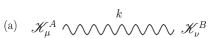
   Figure 1: Feynman rules for propagators: (a) massive vector propagator, (b) FP ghost propagator, (c) NL field propagator.

   

   

   

   

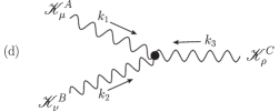
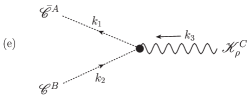
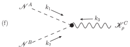
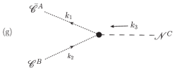
   Figure 2: Feynman rules for three-point vertex functions: (d) $\mathscr{K}\mathscr{K}\mathscr{K}$ vertex, (e) $\mathscr{K}\mathscr{C}\bar{\mathscr{C}}$ vertex, (f) $\mathscr{K}\mathscr{N}\mathscr{N}$ vertex, (g) $\mathscr{N}\mathscr{C}\bar{\mathscr{C}}$ vertex.

   Three-point vertices (Fig. 2)
   

4. $\mathscr{K}\mathscr{K}\mathscr{K}$ vertex $\langle\mathscr{K}^{A}_{\mu}(k_{1})\mathscr{K}^{B}_{\nu}(k_{2})\mathscr{K}^{C}_{\rho}(k_{3})\rangle$

   $$-igf^{ABC}V_{\mu\nu\rho}(k_{1},k_{2},k_{3}),$$ (44)

   with

   $$V_{\mu\nu\rho}(k_{1},k_{2},k_{3}):= (k_{1}-k_{2})_{\rho}g_{\mu\nu}+(k_{2}-k_{3})_{\mu}g_{\nu\rho}$$

   $$+(k_{3}-k_{1})_{\nu}g_{\rho\mu}.$$ (45)

5. $\mathscr{K}\mathscr{C}\bar{\mathscr{C}}$ vertex $\langle\bar{\mathscr{C}}^{A}(k_{1})\mathscr{C}^{B}(k_{2})\mathscr{K}^{C}_{\rho}(k_{3})\rangle$

   $$-igf^{ABC}\{M^{-2}[k_{1\rho}(k_{2}\cdot k_{3})-k_{2\rho}(k_{1}\cdot k_{3})]$$

   $$+k_{1\rho}-k_{2\rho}\}.$$ (46)

6. $\mathscr{K}\mathscr{N}\mathscr{N}$ vertex $\langle\mathscr{N}^{A}(k_{1})\mathscr{N}^{B}(k_{2})\mathscr{K}^{C}_{\rho}(k_{3})\rangle$

   $$igM^{-2}f^{ABC}\{M^{-2}[k_{1\rho}(k_{2}\cdot k_{3})-k_{2\rho}(k_{1}\cdot k_{3})]$$

   $$+k_{1\rho}-k_{2\rho}\}.$$ (47)

7. $\mathscr{N}\mathscr{C}\bar{\mathscr{C}}$ vertex $\langle\bar{\mathscr{C}}^{A}(k_{1})\mathscr{C}^{B}(k_{2})\mathscr{N}^{C}(k_{3})\rangle$

   $$igf_{ABC}[M^{-2}k_{1}\cdot k_{3}-\beta/2].$$ (48)

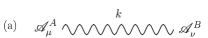
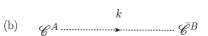
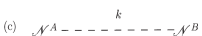
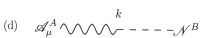
Figure 3: Feynman rules for propagators: (a) massive vector propagator, (b) FP ghost propagator, (c) NL field propagator, (d) cross propagator.

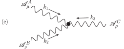
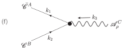
Figure 4: Feynman rules for three-point vertex functions: (e) $\mathscr{A}\mathscr{A}\mathscr{A}$ vertex, (f) $\mathscr{A}\mathscr{C}\bar{\mathscr{C}}$ vertex.

These rules should be compared with the following Feynman rules for the original Lagrangian.
Propagators (Fig. 3)

1. Vector propagator $\langle{\mathscr{A}}^{A}_{\mu}(k){\mathscr{A}}^{B}_{\nu}(-k)\rangle$

   $$-\frac{i}{k^{2}-M^{2}+i\varepsilon}\left(g_{\mu\nu}-\frac{k_{\mu}k_{\nu}}{k^{2}+i\varepsilon}\right)\delta^{AB}$$

   $$-\frac{i\beta}{k^{2}-\beta M^{2}+i\varepsilon}\frac{k_{\mu}k_{\nu}}{k^{2}+i\varepsilon}\delta^{AB}=D^{AB}_{\mu\nu}(k).$$ (49)

2. FP ghost propagator $\langle{\mathscr{C}}^{A}(k){\bar{\mathscr{C}}}^{B}(-k)\rangle$

   $$-\frac{i}{k^{2}-\beta M^{2}+i\varepsilon}\delta^{AB}.$$ (50)

3. NL field propagator $\langle{\mathscr{N}}^{A}(k){\mathscr{N}}^{B}(-k)\rangle$

   $$\frac{iM^{2}}{k^{2}-\beta M^{2}+i\varepsilon}\delta^{AB}.$$ (51)

4. The cross propagator $\langle{\mathscr{A}}^{A}_{\mu}(k){\mathscr{N}}^{B}(-k)\rangle$

   $$\frac{-k_{\mu}}{k^{2}-\beta M^{2}+i\varepsilon}\delta^{AB}.$$ (52)

   Three-point vertices (Fig. 4)
   

5. $\mathscr{A}\mathscr{A}\mathscr{A}$ vertex $\langle\mathscr{A}_{\mu}^{A}(k_{1})\mathscr{A}_{\nu}^{B}(k_{2})\mathscr{A}_{\rho}^{C}(k_{3})\rangle$

   $$-igf^{ABC}V_{\mu\nu\rho}(k_{1},k_{2},k_{3}),$$ (53)

6. $\mathscr{A}\mathscr{C}\bar{\mathscr{C}}$ vertex $\langle\bar{\mathscr{C}}^{A}(k_{1})\mathscr{C}^{B}(k_{2})\mathscr{A}_{\rho}^{C}(k_{3})\rangle$

   $$igf_{ABC}k_{1\rho}.$$ (54)

From the relation,

$$\mathscr{A}_{\mu}=\mathscr{K}_{\mu}+\frac{1}{M^{2}}\partial_{\mu}\mathscr{N}+O(g),$$ (55)

we find

$$\langle\mathscr{A}_{\mu}(x)\mathscr{A}_{\nu}(y)\rangle$$

$$= \langle(\mathscr{K}_{\mu}(x)+M^{-2}\partial_{\mu}\mathscr{N}(x))(\mathscr{K}_{\nu}(y)+M^{-2}\partial_{\nu}\mathscr{N}(y))\rangle$$

$$= \langle\mathscr{K}_{\mu}(x)\mathscr{K}_{\nu}(y)\rangle+M^{-2}\langle\mathscr{K}_{\mu}(x)\partial_{\nu}\mathscr{N}(y)\rangle$$

$$+M^{-2}\langle\partial_{\mu}\mathscr{N}(x)\mathscr{K}_{\nu}(y)\rangle+M^{-4}\langle\partial_{\mu}\mathscr{N}(x)\partial_{\nu}\mathscr{N}(y)\rangle,$$ (56)

which has the Fourier transform:

$$\langle\tilde{\mathscr{A}}^{A}_{\mu}(k)\tilde{\mathscr{A}}^{B}_{\nu}(-k)\rangle$$

$$= \langle\tilde{\mathscr{K}}^{A}_{\mu}(k)\tilde{\mathscr{K}}^{B}_{\nu}(-k)\rangle+ik_{\nu}M^{-2}\langle\mathscr{K}_{\mu}^{A}(-k)\mathscr{N}^{B}(k)\rangle$$

$$-ik_{\mu}M^{-2}\langle\mathscr{N}^{A}(k)\mathscr{K}_{\nu}^{B}(-k)\rangle$$

$$+M^{-4}k_{\mu}k_{\nu}\langle\mathscr{N}^{A}(k)\mathscr{N}^{B}(-k)\rangle$$

$$= i\delta^{AB}\left[-\frac{g_{\mu\nu}-\frac{k_{\mu}k_{\nu}}{M^{2}}}{k^{2}-M^{2}+i\epsilon}-\frac{\frac{k_{\mu}k_{\nu}}{M^{2}}}{k^{2}-\beta M^{2}+i\epsilon}\right],$$ (57)

where we have used (41) and (49) and the fact that there are no mixing propagators:

$$\langle\mathscr{K}_{\mu}^{A}(-k)\mathscr{N}^{B}(k)\rangle=0=\langle\mathscr{N}^{A}(k)\mathscr{K}_{\nu}^{B}(-k)\rangle.$$ (58)

Thus the original gluon two-point function or propagator is decomposed into the spin-one and spin-sero parts.

Another expression for the propagator is the manifestly (power-counting) renormalizable form:

$$\langle\tilde{\mathscr{A}}^{A}_{\mu}(k)\tilde{\mathscr{A}}^{B}_{\nu}(-k)\rangle$$

$$= i\delta^{AB}\left[-\frac{g_{\mu\nu}-\frac{k_{\mu}k_{\nu}}{k^{2}+i\epsilon}}{k^{2}-M^{2}+i\epsilon}-\frac{\beta\frac{k_{\mu}k_{\nu}}{k^{2}+i\epsilon}}{k^{2}-\beta M^{2}+i\epsilon}\right].$$ (59)

For higher orders, see Appendix B.

V Physical unitarity of massless Yang-Mills theory

The $S$ matrix or the scattering operator $S$ is unitary:

$$\textbf{1}=S^{\dagger}S=SS^{\dagger}.$$ (60)

This means that for any (initial) state $\Psi_{b}\in\mathcal{V}$ and any (final) state $\Psi_{a}\in\mathcal{V}$, the following relation holds:

$$\langle\Psi_{b}|\Psi_{a}\rangle= \langle\Psi_{b}|S^{\dagger}S|\Psi_{a}\rangle=\sum_{\Phi_{n}\in\mathcal{V}}\langle\Psi_{b}|S^{\dagger}|\Phi_{n}\rangle\langle\Phi_{n}|S|\Psi_{a}\rangle,$$ (61)

which is obtained by inserting the complete set of states $\{\Phi_{n}\}$ in the total state space $\mathcal{V}$: $\textbf{1}=\sum_{\Phi_{n}\in\mathcal{V}}|\Phi_{n}\rangle\langle\Phi_{n}|.$

On the other hand, the physical unitarity of the $S$ matrix means that the $S$ matrix is unitary on the physical subspace $\mathcal{V}_{\rm phys}$: for any physical state $\Psi_{a},\Psi_{b}\in\mathcal{V}_{\rm phys}$,

$$\langle\Psi_{b}|\Psi_{a}\rangle=\sum_{\Phi_{n}\in\mathcal{V}_{\rm phys}}\langle\Psi_{b}|S^{\dagger}|\Phi_{n}\rangle\langle\Phi_{n}|S|\Psi_{a}\rangle,$$ (62)

where the physical subspace $\mathcal{V}_{\rm phys}$ is defined by

$$\mathcal{V}_{\rm phys}:=\{|\rm{phys}\rangle\in\mathcal{V};\langle\rm{phys}|\rm{phys}\rangle\geq 0\}\subset\mathcal{V}.$$ (63)

The unitarity of the $S$ matrix is rewritten in terms of the scattering amplitude defined by

$$S={\bm{1}}+iT,$$ (64)

into the relation:

$$-i(T-T^{\dagger})=TT^{\dagger}.$$ (65)

Then the unitarity relation reads that for any state $\Psi_{a},\Psi_{b}\in\mathcal{V}$,

$${\rm Im}\langle\Psi_{b}|T|\Psi_{a}\rangle:= \frac{1}{2i}(\langle\Psi_{b}|T|\Psi_{a}\rangle-\langle\Psi_{b}|T^{\dagger}|\Psi_{a}\rangle)$$

$$= \frac{1}{2}\sum_{\Phi_{n}\in\mathcal{V}}\langle\Psi_{b}|T|\Phi_{n}\rangle\langle\Phi_{n}|T^{\dagger}|\Psi_{a}\rangle.$$ (66)

On the other hand, the physical unitarity requires that for any physical state $\Psi_{a},\Psi_{b}\in\mathcal{V}_{\rm phys}$, only the physical states contribute to the intermediate states:

$${\rm Im}\langle\Psi_{b}|T|\Psi_{a}\rangle=\frac{1}{2}\sum_{\Phi_{n}\in\mathcal{V}_{\rm phys}}\langle\Psi_{b}|T|\Phi_{n}\rangle\langle\Phi_{n}|T^{\dagger}|\Psi_{a}\rangle.$$ (67)

In other words, the physical unitarity in gauge theories states that all the unphysical modes cancel in the intermediate states. The imaginary part is calculated by the Cutkosky cutting rule Cutkosky60 .

As a simple example, we consider a one-particle scattering, i.e., a scattering process $\mathscr{A}\rightarrow\mathscr{A}$ in which the initial state is a massless gluon and the final state is also a massless gluon in the massless Yang-Mills theory as the $M=0$ case of the CF model. The Feynman rules in the $M=0$ case have been given in KMSI02 . In the lowest order of the perturbation theory, the Feynman graphs of this process are given by Fig. 5. Each diagram has one closed loop. The initial state and the final state of a gluon are specified by the polarization vectors:

$$\varepsilon^{(\sigma)\alpha}(k):=\varepsilon^{\alpha},\quad\varepsilon^{(\sigma)\alpha{}^{\prime}}(k):=\varepsilon^{\alpha{}^{\prime}}.$$ (68)

For this process up to the order $g^{2}$, we wish to check the physical unitarity relation for the scattering amplitude $T$. By applying the Cutkosky rule Cutkosky60 to Fig. 5, we find that the imaginary part of the scattering amplitude $T(T^{\pm}\rightarrow T^{\pm})$ from a transverse mode $T^{\pm}$ to a transverse mode $T^{\pm}$ is given by Fig. 6. Here it should be remarked that the tadpole diagram does not have the imaginary part.

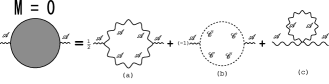
Figure 5: In the massless case $M=0$, the diagrams contributing to the amplitude $T(\mathscr{A}\rightarrow\mathscr{A})$ to the order $g^{2}$ are given by (a) vector boson loop, (b) ghost–antighost loop, (c) boson tadpole.

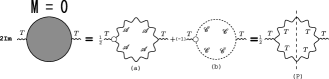
Figure 6: In the massless case $M=0$, the physical unitarity of the amplitude $T(T^{\pm}\rightarrow T^{\pm})$ to the order $g^{2}$ is checked according to the Cutkosky rule using the diagrams: (a) vector boson loop, (b) ghost–antighost loop.

The imaginary part of the diagram Fig. 6(a) with a gluon loop is given by

$$\frac{1}{2} (ig)f_{ABC}V_{\mu\nu\alpha}(k_{1},k_{2},k_{3})$$

$$\times(-ig)f_{ABC^{\prime}}V_{\mu^{\prime}\nu^{\prime}\alpha^{\prime}}(-k_{1},-k_{2},-k_{3})$$

$$\times 2\pi\theta(k_{1}^{0})\delta(k_{1}^{2})g^{\mu\mu^{\prime}}2\pi\theta(k_{2}^{0})\delta(k_{2}^{2})g^{\nu\nu^{\prime}}\varepsilon^{\alpha}(k_{3})\varepsilon^{\alpha^{\prime}}(-k_{3}),$$ (69)

where we have adopted the Feynman gauge $\beta=1$ for the gluon propagator and the factor 1/2 is the symmetrical factor due to two identical particles. This is written as

$$2g^{2}\pi^{2}f_{ABC}f_{ABC^{\prime}}T_{\mu\nu}g^{\mu\mu^{\prime}}g^{\nu\nu^{\prime}}T_{\mu^{\prime}\nu^{\prime}}\theta(k_{1}^{0})\delta(k_{1}^{2})\theta(k_{2}^{0})\delta(k_{2}^{2}),$$ (70)

where we have defined

$$T_{\mu\nu}:=V_{\mu\nu\alpha}(k_{1},k_{2},k_{3})\varepsilon^{\alpha}(k_{3}),$$

$$T_{\mu^{\prime}\nu^{\prime}}:=V_{\mu^{\prime}\nu^{\prime}\alpha^{\prime}}(-k_{1},-k_{2},-k_{3})\varepsilon^{\alpha^{\prime}}(-k_{3}).$$ (71)

In the massless case $M=0$, the physical unitarity requires the imaginary part of the sum of the second-order diagrams to be equal to

$$2g^{2}\pi^{2}f_{ABC}f_{ABC^{\prime}}T_{\mu\nu}P^{\mu\mu^{\prime}}P^{\nu\nu^{\prime}}T_{\mu^{\prime}\nu^{\prime}}$$

$$\times\theta(k_{1}^{0})\delta(k_{1}^{2})\theta(k_{2}^{0})\delta(k_{2}^{2})$$

$$= \frac{1}{2}(ig)f_{ABC}V_{\mu\nu\alpha}(k_{1},k_{2},k_{3})$$

$$\times(-ig)f_{ABC^{\prime}}V_{\mu^{\prime}\nu^{\prime}\alpha^{\prime}}(-k_{1},-k_{2},-k_{3})$$

$$\times 2\pi\theta(k_{1}^{0})\delta(k_{1}^{2})P^{\mu\mu^{\prime}}2\pi\theta(k_{2}^{0})\delta(k_{2}^{2})P^{\nu\nu^{\prime}}\varepsilon^{\alpha}(k_{3})\varepsilon^{\alpha^{\prime}}(-k_{3})$$

$$= \frac{1}{2}\sum_{a,b=1}^{2}(igf_{ABC}V_{\mu\nu\alpha}(k_{1},k_{2},k_{3}))\varepsilon_{a}^{\mu}(k_{1})\varepsilon_{b}^{\nu}(k_{2})\varepsilon^{\alpha}(k_{3})$$

$$\times(igf_{ABC^{\prime}}V_{\mu^{\prime}\nu^{\prime}\alpha^{\prime}}(k_{1},k_{2},k_{3}))^{*}\varepsilon_{a}^{*\mu^{\prime}}(k_{1})\varepsilon_{b}^{*\nu^{\prime}}(k_{2})\varepsilon^{\alpha^{\prime}}(-k_{3})$$

$$\times 2\pi\theta(k_{1}^{0})\delta(k_{1}^{2})2\pi\theta(k_{2}^{0})\delta(k_{2}^{2}),$$ (72)

which is obtained from (70) by the replacement:

$$g^{\mu\mu^{\prime}}\to P^{\mu\mu^{\prime}}=\sum_{a=1}^{2}\varepsilon_{a}^{\mu}(k_{1})\varepsilon_{a}^{*\mu^{\prime}}(k_{1}),$$

$$g^{\nu\nu^{\prime}}\to P^{\nu\nu^{\prime}}=\sum_{b=1}^{2}\varepsilon_{b}^{\nu}(k_{2})\varepsilon_{b}^{*\nu^{\prime}}(k_{2}),$$ (73)

where $P$ correspond to the two transverse polarization states for the massless spin-one modes $T^{\pm}$.

By using the decomposition:

$$g^{\mu\mu^{\prime}} =-P^{\mu\mu^{\prime}}+Q^{\mu\mu^{\prime}},\ Q^{\mu\mu^{\prime}}=(k_{1}^{\mu}\bar{k}_{1}^{\mu^{\prime}}+\bar{k}_{1}^{\mu}k_{1}^{\mu^{\prime}})/(k_{1}\cdot\bar{k}_{1}),$$

$$g^{\nu\nu^{\prime}} =-P^{\nu\nu^{\prime}}+Q^{\nu\nu^{\prime}},\ Q^{\nu\nu^{\prime}}=(k_{2}^{\nu}\bar{k}_{2}^{\nu^{\prime}}+\bar{k}_{2}^{\nu}k_{2}^{\nu^{\prime}})/(k_{2}\cdot\bar{k}_{2}),$$ (74)

the difference between (69)=(70) and (72) is calculated from

$$g^{\mu\mu^{\prime}}g^{\nu\nu^{\prime}}-P^{\mu\mu^{\prime}}P^{\nu\nu^{\prime}}$$

$$= -P^{\mu\mu^{\prime}}Q^{\nu\nu^{\prime}}-P^{\nu\nu^{\prime}}Q^{\mu\mu^{\prime}}+Q^{\mu\mu^{\prime}}Q^{\nu\nu^{\prime}},$$ (75)

where $Q$ are rewritten using the polarization vectors for the longitudinal (L) and the scalar (S) modes:

$$Q^{\mu\mu^{\prime}}=\varepsilon_{L}^{\mu}(k_{1})\varepsilon_{S}^{*\mu^{\prime}}(k_{1})+\varepsilon_{S}^{\mu}(k_{1})\varepsilon_{L}^{*\mu^{\prime}}(k_{1}),$$

$$Q^{\nu\nu^{\prime}}=\varepsilon_{L}^{\nu}(k_{2})\varepsilon_{S}^{*\nu^{\prime}}(k_{2})+\varepsilon_{S}^{\nu}(k_{2})\varepsilon_{L}^{*\nu^{\prime}}(k_{2}).$$ (76)

By using the relationships:

$$T_{\mu\nu}\varepsilon_{\sigma}^{\mu}(k_{1})\varepsilon_{L}^{\nu}(k_{2})=T_{\mu\nu}\varepsilon_{L}^{\mu}(k_{1})\varepsilon_{\sigma}^{\nu}(k_{2})$$

$$=\begin{cases}(-i)k_{1\alpha}\varepsilon^{\alpha}(k_{3})\quad&(\sigma=S)\\ 0\quad&(\sigma=T,L)\end{cases},$$ (77)

and

$$T_{\mu^{\prime}\nu^{\prime}}\varepsilon_{\sigma}^{*\mu^{\prime}}(k_{1})\varepsilon_{L}^{*\nu^{\prime}}(k_{2})=T_{\mu^{\prime}\nu^{\prime}}\varepsilon_{L}^{*\mu^{\prime}}(k_{1})\varepsilon_{\sigma}^{*\nu^{\prime}}(k_{2})$$

$$=\begin{cases}ik_{1\alpha^{\prime}}\varepsilon^{\alpha^{\prime}}(-k_{3})\quad&(\sigma=S)\\ 0\quad&(\sigma=T,L)\end{cases},$$ (78)

we find that the first and second term in the right-hand side of (75) give vanishing contributions.

The relationship (77) is derived as follows. First, we find

$$V_{\mu\nu\alpha}(k_{1},k_{2},k_{3})\varepsilon_{L}^{\nu}(k_{2})$$

$$= V_{\mu\nu\alpha}(k_{1},k_{2},k_{3})k^{\nu}_{2}$$

$$= (k_{1}-k_{2})_{\alpha}k_{2\mu}+(k_{2}-k_{3})_{\mu}k_{2\alpha}+(k_{3}\cdot k_{2}-k_{1}\cdot k_{2})g_{\alpha\mu}$$

$$= -k_{1\alpha}k_{1\mu}+k_{3\alpha}k_{3\mu},$$ (79)

where we have used $k_{1}^{2}=0$ and $k_{3}^{2}=0$ for the massless on-shell momenta. Then we have

$$V_{\mu\nu\alpha}(k_{1},k_{2},k_{3})\varepsilon_{\sigma}^{\mu}(k_{1})\varepsilon_{L}^{\nu}(k_{2})\varepsilon^{\alpha}(k_{3})$$

$$= -k_{1\alpha}\varepsilon^{\alpha}(k_{3})k_{1\mu}\varepsilon_{\sigma}^{\mu}(k_{1})+k_{3\alpha}\varepsilon^{\alpha}(k_{3})k_{3\mu}\varepsilon_{\sigma}^{\mu}(k_{1}),$$ (80)

where $k_{3\alpha}\varepsilon^{\alpha}(k_{3})=0$ for the physical transverse mode, while $k_{1\mu}\varepsilon_{T}^{\mu}(k_{1})=0$, $k_{1\mu}\varepsilon_{L}^{\mu}(k_{1})=-ik_{1\mu}k_{1}^{\mu}=0$ for massless on-shell $k_{1}$, and $k_{1\mu}\varepsilon_{S}^{\mu}(k_{1})=i$ for massless on-shell $k_{1}$.

Thus, only the last term in (75) gives a nonvanishing contribution:

$$4g^{2}\pi^{2}f_{ABC}f_{ABC^{\prime}}k_{1\alpha}\varepsilon^{\alpha}(k_{3})k_{1\alpha^{\prime}}\varepsilon^{\alpha^{\prime}}(-k_{3})$$

$$\times\theta(k_{1}^{0})\delta(k_{1}^{2})\theta(k_{2}^{0})\delta(k_{2}^{2}).$$ (81)

This difference is exactly provided by the imaginary part of the second diagram of Fig.6(b) with a ghost loop:

$$(-1)(-igf_{ABC}k_{1\alpha})(igf_{ABC^{\prime}}k_{1\alpha^{\prime}})\varepsilon^{\alpha}(k_{3})\varepsilon^{\alpha^{\prime}}(-k_{3})$$

$$\times 2\pi\theta(k_{1}^{0})\delta(k_{1}^{2})2\pi\theta(k_{2}^{0})\delta(k_{2}^{2})$$

$$= -4g^{2}\pi^{2}f_{ABC}f_{ABC^{\prime}}k_{1\alpha}\varepsilon^{\alpha}(k_{3})k_{1\alpha^{\prime}}\varepsilon^{\alpha^{\prime}}(-k_{3})$$

$$\times\theta(k_{1}^{0})\delta(k_{1}^{2})\theta(k_{2}^{0})\delta(k_{2}^{2}),$$ (82)

where we have used the original gluon-ghost-antighost vertex (given in KMSI02 at $\xi=1/2$ corresponding to $\alpha=0$), $\frac{1}{2}igf_{ABC}(k_{1\alpha}-k_{2\alpha})=igf_{ABC}(k_{1\alpha}+\frac{1}{2}k_{3\alpha})$, and the property of polarization vectors, $k_{3\alpha}\varepsilon^{\alpha}(k_{3})=0$, to obtain the first expression. Thus, the unitarity relation is satisfied in the massless case $M=0$.

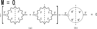
Figure 7: In the massless case $M=0$, mode cancellations occur to ensure the physical unitarity for the one-particle amplitude $T(T^{\pm}\rightarrow T^{\pm})$ for the transverse mode $T$ to the order $g^{2}$. In the amplitude, two diagrams (a) from the longitudinal mode $L$ and the scalar mode $S$ are canceled by a ghost-antighost $\mathscr{C},\mathscr{\bar{C}}$ diagram (b).

The physical unitarity is ensured by mode cancellations. See Fig. 7. The contributions from the longitudinal mode $L$ and the scalar mode $S$ are canceled by a ghost-antighost $\mathscr{C},\mathscr{\bar{C}}$ one.

VI Physical nonunitarity of massive Yang-Mills theory

In this section, we reproduce the violation of physical unitarity in the massive Yang-Mills theory without the Higgs field based on the conventional argument, which shows the utility of the massive field $\mathscr{K}$ in discussing the physical unitarity of the CF model in the next section.

In order to see a difference between massless gauge theory ($M=0$) and massive vector theory ($M\not=0$), we consider the one-particle scattering, i.e., a scattering process $U\rightarrow U$ in which the initial state is a massive vector boson and the final state is also a massive vector boson. Here $U_{\mu}$ is defined by

$$U_{\mu}:=\mathscr{A}_{\mu}-\frac{1}{M^{2}}\partial_{\mu}\mathscr{N},\quad\text{or}\quad\mathscr{A}_{\mu}=U_{\mu}+\frac{1}{M^{2}}\partial_{\mu}\mathscr{N}.$$ (83)

In the lowest order of the perturbation theory, the Feynman diagrams of this process are given by the same graphs as those in Fig. 5 where the propagators are replaced by the massive ones and the vertex functions are unchanged. Therefore, the imaginary part is given by the diagrams of Fig. 8.

The imaginary part of the diagram Fig. 8(a) with a loop of massive vector boson is

$$\frac{1}{2}(-ig)f_{ABC}V_{\mu\nu\alpha}(k_{1},k_{2},k_{3})$$

$$\times(ig)f_{ABC^{\prime}}V_{\mu^{\prime}\nu^{\prime}\alpha^{\prime}}(-k_{1},-k_{2},-k_{3})$$

$$\times 2\pi\theta(k_{1}^{0})\delta(k_{1}^{2}-M^{2})g^{\mu\mu^{\prime}}$$

$$\times 2\pi\theta(k_{2}^{0})\delta(k_{2}^{2}-M^{2})g^{\nu\nu^{\prime}}\varepsilon^{\alpha}(k_{3})\varepsilon^{\alpha^{\prime}}(-k_{3}),$$ (84)

where the factor 1/2 is the symmetrical factor due to two identical particles. The imaginary part (84) is written as

$$2g^{2}\pi^{2}f_{ABC}f_{ABC^{\prime}}T_{\mu\nu}g^{\mu\mu^{\prime}}g^{\nu\nu^{\prime}}T_{\mu^{\prime}\nu^{\prime}}$$

$$\times\theta(k_{1}^{0})\delta(k_{1}^{2}-M^{2})\theta(k_{2}^{0})\delta(k_{2}^{2}-M^{2}),$$ (85)

where we have defined

$$T_{\mu\nu}:=V_{\mu\nu\alpha}(k_{1},k_{2},k_{3})\varepsilon^{\alpha}(k_{3}),$$

$$T_{\mu^{\prime}\nu^{\prime}}:=V_{\mu^{\prime}\nu^{\prime}\alpha^{\prime}}(-k_{1},-k_{2},-k_{3})\varepsilon^{\alpha^{\prime}}(-k_{3}).$$ (86)

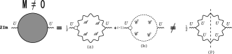
Figure 8: In the massive case $M\not=0$, the physical unitarity of the amplitude $T(U\rightarrow U)$ for the physical spin-one vector mode $U$ to the order $g^{2}$ is checked according to the Cutkosky rule using the diagrams: (a) vector boson loop, (b) ghost–antighost loop. The physical unitarity is violated due to the incomplete cancellation.

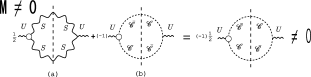
Figure 9: In the massive case $M\not=0$, the incomplete mode cancellation among unphysical modes to the order $g^{2}$ prevents us from ensuring the physical unitarity for the one-particle amplitude $T(U\rightarrow U)$ for the physical spin-one vector mode $U$. In the amplitude, a diagram (a) from the scalar mode $S$ is overcanceled by a ghost-antighost diagram (b), leaving one-half of (b) nonvanishing.

In the massive case $M\neq 0$, the physical unitarity requires the imaginary part of the second-order diagram to be equal to

$$2g^{2}\pi^{2}f_{ABC}f_{ABC^{\prime}}T_{\mu\nu}P^{\mu\mu^{\prime}}P^{\nu\nu^{\prime}}T_{\mu^{\prime}\nu^{\prime}}$$

$$\times\theta(k_{1}^{0})\delta(k_{1}^{2}-M^{2})\theta(k_{2}^{0})\delta(k_{2}^{2}-M^{2})$$

$$= \frac{1}{2}(igf_{ABC}T_{\mu\nu}\varepsilon^{\mu}_{j}(k_{1})\varepsilon^{\nu}_{\ell}(k_{2}))$$

$$\times(igf_{ABC^{\prime}}T_{\mu^{\prime}\nu^{\prime}}\varepsilon^{\mu^{\prime}}_{j}(k_{1})\varepsilon^{\nu^{\prime}}_{\ell}(k_{2}))^{*}$$

$$\times 2\pi\theta(k_{1}^{0})\delta(k_{1}^{2}-M^{2})2\pi\theta(k_{2}^{0})\delta(k_{2}^{2}-M^{2}),$$ (87)

which is obtained from (85) by the replacement:

$$g^{\mu\mu^{\prime}}\to P^{\mu\mu^{\prime}}=\sum_{j=1}^{3}\varepsilon^{\mu}_{(j)}(k_{1})\varepsilon^{\mu^{\prime}}_{(j)}(k_{1}),$$

$$g^{\nu\nu^{\prime}}\to P^{\nu\nu^{\prime}}=\sum_{j=1}^{3}\varepsilon^{\nu}_{(j)}(k_{2})\varepsilon^{\nu^{\prime}}_{(j)}(k_{2}).$$ (88)

Using the decomposition for $M\not=0$:

$$g^{\mu\mu^{\prime}}=-P^{\mu\mu^{\prime}}+\frac{k_{1}^{\mu}k_{1}^{\mu^{\prime}}}{M^{2}},\quad g^{\nu\nu^{\prime}}=-P^{\nu\nu^{\prime}}+\frac{k_{2}^{\nu}k_{2}^{\nu^{\prime}}}{M^{2}},$$ (89)

where $P$ selects three polarization states ($T^{+},T^{-},L$) for the massive spin-one boson $U$, the difference between (84)=(85) and (87) is calculated from

$$g^{\mu\mu^{\prime}}g^{\nu\nu^{\prime}}-P^{\mu\mu^{\prime}}P^{\nu\nu^{\prime}}$$

$$= -P^{\mu\mu^{\prime}}\frac{k_{2}^{\nu}k_{2}^{\nu^{\prime}}}{M^{2}}-P^{\nu\nu^{\prime}}\frac{k_{1}^{\mu}k_{1}^{\mu^{\prime}}}{M^{2}}+\frac{k_{1}^{\mu}k_{1}^{\mu^{\prime}}}{M^{2}}\frac{k_{2}^{\nu}k_{2}^{\nu^{\prime}}}{M^{2}}.$$ (90)

The contribution from the first term of the right-hand side of (90) to (85) is given by

$$2g^{2}\frac{1}{M^{2}}\pi^{2}f_{ABC}f_{ABC^{\prime}}T_{\mu\nu}\varepsilon^{\mu}_{j}(k_{1})k_{2}^{\nu}\varepsilon^{\mu^{\prime}}_{j}(k_{1})k_{2}^{\nu^{\prime}}T_{\mu^{\prime}\nu^{\prime}}$$

$$\times\theta(k_{1}^{0})\delta(k_{1}^{2}-M^{2})\theta(k_{2}^{0})\delta(k_{2}^{2}-M^{2}).$$ (91)

This is zero, since

$$T_{\mu\nu}\varepsilon^{\mu}_{j}(k_{1})k_{2}^{\nu}$$

$$=\varepsilon^{\mu}_{j}(k_{1})V_{\mu\nu\alpha}(k_{1},k_{2},k_{3})k_{2}^{\nu}\varepsilon^{\alpha}(k_{3})$$

$$=\varepsilon^{\mu}_{j}(k_{1})[-k_{1\mu}k_{1\alpha}+k_{3\mu}k_{3\alpha}+k_{1}^{2}g_{\mu\alpha}-k_{3}^{2}g_{\mu\alpha}]\varepsilon^{\alpha}(k_{3})$$

$$=-k_{1\mu}\varepsilon^{\mu}_{j}(k_{1})k_{1\alpha}\varepsilon^{\alpha}(k_{3})+k_{3\mu}\varepsilon^{\mu}_{j}(k_{1})k_{3\alpha}\varepsilon^{\alpha}(k_{3})$$

$$=0,$$ (92)

where we have used $k_{1}^{2}=k_{3}^{2}$ and $k_{\mu}\varepsilon^{\mu}_{(j)}(k)=0$. Similarly, the contribution from the second term of (90) is vanishing. The third term of (90) gives

$$2g^{2}\pi^{2}f_{ABC}f_{ABC^{\prime}}T_{\mu\nu}\frac{k_{1}^{\mu}k_{2}^{\nu}}{M^{2}}\frac{k_{1}^{\mu^{\prime}}k_{2}^{\nu^{\prime}}}{M^{2}}T_{\mu^{\prime}\nu^{\prime}}.$$ (93)

Using the property:

$$T_{\mu\nu}k_{1}^{\mu}k_{2}^{\nu} =-k_{1}^{2}k_{1\alpha}\varepsilon^{\alpha}(k_{3})+k_{1}\cdot k_{3}k_{3\alpha}\varepsilon^{\alpha}(k_{3})$$

$$=-M^{2}k_{1\alpha}\varepsilon^{\alpha}(k_{3}),$$ (94)

we obtain the difference:

$$2g^{2}\pi^{2}f_{ABC}f_{ABC^{\prime}}k_{1\alpha}\varepsilon^{\alpha}(k_{3})k_{1\alpha^{\prime}}\varepsilon^{\alpha^{\prime}}(-k_{3})$$

$$\times\theta(k_{1}^{0})\delta(k_{1}^{2}-M^{2})\theta(k_{2}^{0})\delta(k_{2}^{2}-M^{2}).$$ (95)

This difference must be provided by the imaginary part of the diagram Fig. 8(b) with a loop of massive ghost which is given by

$$(-1)\varepsilon^{\alpha}(k_{3})\varepsilon^{\alpha^{\prime}}(-k_{3})(-igf_{ABC}k_{1\alpha})(igf_{ABC^{\prime}}(-k_{2\alpha^{\prime}}))$$

$$\times 2\pi\theta(k_{1}^{0})\delta(k_{1}^{2}-M^{2})2\pi\theta(k_{2}^{0})\delta(k_{2}^{2}-M^{2})$$

$$= -4g^{2}\pi^{2}f_{ABC}f_{ABC^{\prime}}k_{1\alpha}\varepsilon^{\alpha}(k_{3})k_{1\alpha^{\prime}}\varepsilon^{\alpha^{\prime}}(-k_{3})$$

$$\times\theta(k_{1}^{0})\delta(k_{1}^{2}-M^{2})\theta(k_{2}^{0})\delta(k_{2}^{2}-M^{2}),$$ (96)

where we have used $k_{2}=-k_{1}-k_{3}$ and $k_{3\alpha}\varepsilon^{\alpha}(k_{3})=0$. The ghost contribution (96) is precisely of the same form as (95) and comes with the opposite sign. However, the massive vector contribution (95) cancels against half the massive ghost contribution (96). See Fig.9.

Thus, it is found that there is a discrete difference between massless theories and massive theories. This means that the massless theory cannot be obtained as a limiting case of the massive theory. The origin of the difference goes back to the difference between the sum over polarizations. In the next section, we re-examine the physical unitarity in the the CF model based on our method.

VII Perturbative analysis of physical unitarity in the CF model

In order to re-examine the physical unitarity in the massive Yang-Mills theory, i.e., the CF model, we consider the simplest case of the one-particle amplitude $T(\mathscr{K}\rightarrow\mathscr{K})$ in the perturbation theory, as considered in DV70 .

According to the Cutkosky rules, the physical unitarity up to the order $g^{2}$ is checked by calculating the diagrams in Fig. 10 with one closed loop.

The imaginary part for the diagram Fig. 10(a) is

$$(\rm{a})_{\alpha\alpha^{\prime}}^{CC^{\prime}}:= \left(\frac{1}{2}\right)(ig)f_{ABC}V^{\mu\nu\alpha}(k_{1},k_{2},k_{3})$$

$$\times(-ig)f_{A^{\prime}B^{\prime}C^{\prime}}V^{\mu^{\prime}\nu^{\prime}\alpha^{\prime}}(-k_{1},-k_{2},-k_{3})$$

$$\times 2\pi\theta(k_{1}^{0})\delta^{AA^{\prime}}I_{\mu\mu^{\prime}}(k_{1})2\pi\theta(k_{2}^{0})\delta^{BB^{\prime}}I_{\nu\nu^{\prime}}(k_{2}),$$ (97)

where we have defined

$$I_{\mu\nu}(k):= \delta(k^{2}-M^{2})\left(g_{\mu\nu}-\frac{k_{\mu}k_{\nu}}{M^{2}}\right).$$ (98)

Remember that the three polarization vectors $\varepsilon_{\mu}^{(j)}(k)(j=1,2,3)$ for the spin-one massive vector field $\mathscr{K}_{\mu}$ obey the relation:

$$\sum_{j=1}^{3}\varepsilon_{\mu}^{(j)}(k_{1})\varepsilon_{\mu^{\prime}}^{(j)*}(k_{1})=-g_{\mu\mu^{\prime}}+\frac{k_{1\mu}k_{1\mu^{\prime}}}{M^{2}},$$

$$\sum_{j=1}^{3}\varepsilon_{\nu}^{(j)}(k_{2})\varepsilon_{\nu^{\prime}}^{(j)*}(k_{2})=-g_{\nu\nu^{\prime}}+\frac{k_{2\nu}k_{2\nu^{\prime}}}{M^{2}}.$$ (99)

Therefore, (a) is a physical contribution coming from the spin-one massive vector boson $\mathscr{K}$. The physical unitarity requires that the contributions other than (a), i.e., the contributions (b) and (c) from the unphysical fields $\mathscr{C},\bar{\mathscr{C}}$ and $\mathscr{N}$ are canceled in the same order of the coupling. Therefore, we consider the contributions from unphysical fields.

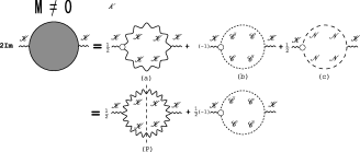
Figure 10: In the massive case $M\not=0$, the physical unitarity of the amplitude $T(\mathscr{K}\rightarrow\mathscr{K})$ to the order $g^{2}$ is checked according to the Cutkosky rule using the diagrams: (a) massive vector boson, (b) ghost–antighost, (c) NL field.

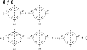
Figure 11: In the massive case $M\not=0$, incomplete mode cancellations violate the physical unitarity for the one-particle amplitude to the order $g^{2}$.

The imaginary part for the diagram Fig. 10(b) with a closed loop of the massive FP ghost and antighost reads

$$(b)_{\alpha\alpha^{\prime}}^{CC^{\prime}}$$

$$:= (-1)(-ig)f_{ABC}\{M^{-2}V_{\alpha}(k_{1},k_{2},k_{3})+k_{1\alpha}-k_{2\alpha}\}$$

$$\times igf_{A^{\prime}B^{\prime}C^{\prime}}\{M^{-2}V_{\alpha^{\prime}}(k_{1},k_{2},k_{3})+k_{1\alpha^{\prime}}-k_{2\alpha^{\prime}}\}$$

$$\times 2\pi\theta(k_{1}^{0})\delta(k_{1}^{2}-\beta M^{2})2\pi\theta(k_{2}^{0})\delta(k_{2}^{2}-\beta M^{2})$$

$$= -4g^{2}\pi^{2}f_{ABC}f_{ABC^{\prime}}\{M^{-2}V_{\alpha}(k_{1},k_{2},k_{3})+k_{1\alpha}-k_{2\alpha}\}$$

$$\times\{\alpha\to\alpha^{\prime}\}\theta(k_{1}^{0})\delta(k_{1}^{2}-\beta M^{2})\theta(k_{2}^{0})\delta(k_{2}^{2}-\beta M^{2}).$$ (100)

The imaginary part of the diagram (c) with a closed loop of the NL field reads

$$(c)_{\alpha\alpha^{\prime}}^{CC^{\prime}}$$

$$:= \left(\frac{1}{2}\right)(-i)\frac{g}{M^{2}}f_{ABC}\{M^{-2}V_{\alpha}(k_{1},k_{2},k_{3})+k_{1\alpha}-k_{2\alpha}\}$$

$$\times i\frac{g}{M^{2}}f_{A^{\prime}B^{\prime}C^{\prime}}\{M^{-2}V_{\alpha^{\prime}}(k_{1},k_{2},k_{3})+k_{1\alpha^{\prime}}-k_{2\alpha^{\prime}}\}$$

$$\times M^{2}2\pi\theta(k_{1}^{0})\delta(k_{1}^{2}-\beta M^{2})\delta^{AA^{\prime}}M^{2}$$

$$\times 2\pi\theta(k_{2}^{0})\delta(k_{2}^{2}-\beta M^{2})\delta^{BB^{\prime}}$$

$$= 2g^{2}\pi^{2}f_{ABC}f_{ABC^{\prime}}\{M^{-2}V_{\alpha}(k_{1},k_{2},k_{3})+k_{1\alpha}-k_{2\alpha}\}$$

$$\times\{\alpha\to\alpha^{\prime}\}\theta(k_{1}^{0})\delta(k_{1}^{2}-\beta M^{2})\theta(k_{2}^{0})\delta(k_{2}^{2}-\beta M^{2}).$$ (101)

Hence, adding the NL loop (c) to the ghost loop (b) yields the half of (b): $(b)+(c)=\frac{1}{2}(b)$, since $(c)=-\frac{1}{2}(b)$. Therefore, we have shown the CF model does not satisfy the physical unitarity for the $M\not=0$ case independently from $\beta$ in the perturbation theory. The incomplete cancellations of the unphysical modes against the physical unitarity are summarized in Fig. 11. This result should be compared with the massless case where the physical modes in the massless case $M=0$ are the two transverse parts.

In the massless case $M=0$, for the amplitude $T\rightarrow T$ of the transverse mode $T^{\pm}$, two diagrams (a) from the longitudinal mode $L$ and the scalar mode $S$ are canceled by a ghost-antighost $\mathscr{C},\mathscr{\bar{C}}$ diagram (b). The NL mode $\mathscr{N}$ is nonpropagating in the massless case and does not contribute to this cancellation.

In the massive case $M\not=0$, for the amplitude $\mathscr{K}\rightarrow\mathscr{K}$ of a physical particle $\mathscr{K}$, a diagram (a) from the scalar mode $S$ (= the NL mode $\mathscr{N}$) is not sufficient to cancel the ghost-antighost $\mathscr{C},\mathscr{\bar{C}}$ diagram (b). An additional bosonic contribution is necessary to realize the complete cancellation.

In the massless case $M=0$, the physical modes are given by two transverse modes $T^{\pm}$. Then the two unphysical modes in the gluon, i.e., the longitudinal mode $L$ and the scalar mode $S$ are canceled by a ghost and antighost $\mathscr{C},\mathscr{\bar{C}}$. Two bosonic modes are exactly canceled by two fermionic (anticommuting) modes. It should be remarked that the scalar mode is identified with the NL mode $\mathscr{N}$, which is non-propagating in the massless case.

$$\framebox{ $T^{+}$, $T^{-}$},L,S(=\mathscr{N}:{\rm nonpropagating});\mathscr{C},\mathscr{\bar{C}}$$ (102)

In the massive case $M\not=0$, the physical modes are given by a longitudinal and two transverse modes. A remaining unphysical mode, i.e., a scalar mode is not sufficient to cancel the ghost and antighost contributions. Therefore, the elementary fields in the original action of the CF model are not sufficient to respect the physical unitarity. There must be a mechanism which supplies the CF model with an extra (bosonic) mode. (Note that the NL field $\mathscr{N}$ is propagating in the massive case and therefore the NL mode is expected to play the important role in the cancellation in the massive case, in sharp contrast to the massless case. However, the NL mode is identical to the scalar mode on mass shell and hence cannot be counted as another independent field.)

$$\framebox{ $T^{+}$, $T^{-}$, $L$},S=\mathscr{N};\mathscr{C},\mathscr{\bar{C}}.$$ (103)

Finally, we discuss how to avoid the violation of physical unitarity. The violation of the physical unitarity is avoided by restricting the relevant energy to the low-energy region such that the ghost and antighost pair cannot be created. This can be done by adjusting the parameter in the CF model. Since the ghost and antighost have the same mass $\sqrt{\beta}M$, the allowed region is

$$E<2\sqrt{\beta}M,\quad E^{2}<4\beta M^{2}.$$ (104)

A shortcoming of this scenario is that $\beta=0$ is not allowed to maintain physical unitarity, since the results of numerical simulations on the lattice are available only in this case $\beta=0$.

At first glance, the cancellation of unphysical modes works well even in the massive case by using the argument similar to that done in the gauge-Higgs model with the renormalizable $R_{\xi}$ gauge. The pole masses of unphysical fields $\mathscr{C},\mathscr{\bar{C}},\mathscr{N}$ are the same:

$$m_{\mathscr{C}}^{2}=m_{\mathscr{\bar{C}}}^{2}=m_{\mathscr{N}}^{2}=\beta M^{2}.$$ (105)

In the limit $\beta\rightarrow\infty$, unphysical fields $\mathscr{C},\mathscr{\bar{C}},\mathscr{N}$ decouple from the theory, leaving the physical field $\mathscr{K}_{\mu}$ in the theory. Therefore, it seems that the physical unitarity holds even in the massive case. However, this is not the case, as we have shown in the above. What is wrong in this argument? This argument is based on the fact that $\beta$ is a gauge-fixing parameter and the physics does not depend on this parameter $\beta$, which is indeed shown in the massless case $M=0$. However, even the BRST-invariant quantities depend on $\beta$ for $M\not=0$. Therefore, the physics depends on $\beta$ for $M\not=0$, and the physics for $\beta\rightarrow\infty$ is different from that for $\beta<\infty$. In this sense, the above result, i.e., violation of physical unitarity in the massive case, does not contradict this argument.

In order to maintain the physical unitarity in the massive Yang-Mills theory without the Higgs field, therefore, we need a nonperturbative approach, which will be given in subsequent papers in preparation.

VIII Conclusion and discussion

In order to understand color confinement in QCD in the light of recent developments, we have considered a “massive” Yang-Mills model without the Higgs field, especially, the CF model, since the CF model is regarded as a good low-energy effective theory of QCD and it is much simpler than the refined Gribov-Zwanziger model, see e.g., Kondo12 .

We have examined the physical unitarity of the CF model which is known to be renormalizable. For this purpose, we have used the field $\mathscr{K}_{\mu}^{A}(x)$ with the following properties:

1. $\mathscr{K}$ is invariant under an extended BRST transformation, ${\bm{\delta}}^{\prime}\mathscr{K}_{\mu}(x)=0$ (off shell).

2. $\mathscr{K}$ is divergenceless, $\partial^{\mu}\mathscr{K}_{\mu}(x)=0$ (on shell).

3. $\mathscr{K}$ transforms according to the adjoint representation under color rotation. $\mathscr{K}_{\mu}(x)\to U\mathscr{K}_{\mu}(x)U^{-1}$

4. $\mathscr{K}$ is invariant under the FP conjugation. $\mathscr{K}_{\mu}(x)\to\mathscr{K}_{\mu}(x)$

Thus, we have identified $\mathscr{K}_{\mu}^{A}$ with a physical and massive vector field with correct degrees of freedom as a non-Abelian spin-one massive vector boson. $\mathscr{K}$ is obtained by a nonlinear but local transformation from the original fields in the CF model.

We have checked in a new perturbative treatment whether or not the CF model satisfies the physical unitarity. Then we have confirmed the violation of the physical unitarity in the perturbative treatment and we have clarified the reason in the massive Yang-Mills theory without the Higgs field. The perturbative analysis for the physical unitarity imposea a restriction on the valid energy together with the parameter of the CF model: $E^{2}<4\beta M^{2}$ in order to confine unphysical modes (ghost, antighost, scalar mode). However, $\beta=0$ is not allowed in this scenario.

The conclusion obtained in this paper still leaves a possibility that the nonperturbative approach can modify the conclusion. In a subsequent paper, indeed, we will propose a scenario in which the physical unitarity can be recovered in the CF model thanks to the FP conjugation invariance. Indeed, we will show that the norm cancellation is automatically guaranteed from the Slavnov-Taylor identities if the ghost-antighost bound state exists. In this way, the physical unitarity can be recovered in a nonperturbative way. To show the existence of the bound state of ghost and antighost, the Nambu-Bethe-Salpeter equation is to be solved. This is a hard work to be tackled in subsequent papers.

Acknowledgements: The authors would like to thank Professor T. Kugo for very enlightening discussion about some issues. This work is supported by Grant-in-Aid for Scientific Research (C) 24540252 from the Japan Society for the Promotion of Science (JSPS).

Appendix A Change of variables

The original theory is given by

$$Z_{\rm mYM}=\int\mathcal{D}\mathscr{A}\mathcal{D}\mathscr{C}\mathcal{D}\mathscr{\bar{C}}\mathcal{D}\mathscr{N}e^{iS^{\rm tot}_{\rm mYM}[\mathscr{A},\mathscr{C},\mathscr{\bar{C}},\mathscr{N}]}.$$ (106)

The exact change of variables, $\mathscr{A}_{\mu},\mathscr{C},\bar{\mathscr{C}},\mathscr{N}\rightarrow\mathscr{K}_{\mu},\mathscr{C},\bar{\mathscr{C}},\mathscr{N}$, could be performed through the relationship $\mathscr{A}=\mathscr{\tilde{A}}[\mathscr{K}_{\mu},\mathscr{C},\bar{\mathscr{C}},\mathscr{N}]$ according to

$$Z_{\rm mYM} =\int\mathcal{D}\mathscr{K}\mathcal{D}\mathscr{C}\mathcal{D}\mathscr{\bar{C}}\mathcal{D}\mathscr{N}\Big{|}\frac{\partial(\mathscr{\tilde{A}})}{\partial(\mathscr{K})}\Big{|}e^{iS^{\rm tot}_{\rm mYM}[\mathscr{\tilde{A}},\mathscr{C},\mathscr{\bar{C}},\mathscr{N}]}$$

$$=\int\mathcal{D}\mathscr{K}\mathcal{D}\mathscr{C}\mathcal{D}\mathscr{\bar{C}}\mathcal{D}\mathscr{N}e^{iS^{\rm tot}_{\rm mYM}[\mathscr{K},\mathscr{C},\mathscr{\bar{C}},\mathscr{N}]},$$ (107)

where

$$S^{\rm tot}_{\rm mYM}[\mathscr{K},\mathscr{C},\mathscr{\bar{C}},\mathscr{N}]:=S^{\rm tot}_{\rm mYM}[\mathscr{\tilde{A}},\mathscr{C},\mathscr{\bar{C}},\mathscr{N}]-i\ln J,$$ (108)

where $J$ is the Jacobian associated with the change of variables from $\mathscr{A}_{\mu},\mathscr{C},\bar{\mathscr{C}},\mathscr{N}$ in the original Lagrangian to $\mathscr{K}_{\mu},\mathscr{C},\bar{\mathscr{C}},\mathscr{N}$ in the new theory.

We proceed to check the modified BRST (mBRST) invariance of the new theory. The action is mBRST invariant by construction. We have already shown that the integration measure $\mathcal{D}\mathscr{A}\mathcal{D}\mathscr{C}\mathcal{D}\mathscr{\bar{C}}\mathcal{D}\mathscr{N}$ is mBRST invariant. The mBRST invariance of the measure $\mathcal{D}\mathscr{K}\mathcal{D}\mathscr{C}\mathcal{D}\mathscr{\bar{C}}\mathcal{D}\mathscr{N}$ is also checked in the same way. Therefore, the Jacobian $J$ must be mBRST invariant too, i.e., ${\bm{\delta}}^{\prime}J=0$.

However, we do not know the exact expression of $\mathscr{A}=\mathscr{\tilde{A}}[\mathscr{K}_{\mu},\mathscr{C},\bar{\mathscr{C}},\mathscr{N}]$ as a functional of $\mathscr{K}_{\mu},\mathscr{C},\bar{\mathscr{C}},\mathscr{N}$, although we know the exact expression of $\mathscr{K}=\mathscr{\tilde{K}}[\mathscr{A}_{\mu},\mathscr{C},\bar{\mathscr{C}},\mathscr{N}]$ as a functional of $\mathscr{A}_{\mu},\mathscr{C},\bar{\mathscr{C}},\mathscr{N}$ as given in (29). We know just the order by order relation for $\mathscr{A}=\mathscr{\tilde{A}}[\mathscr{K}_{\mu},\mathscr{C},\bar{\mathscr{C}},\mathscr{N}]$ as given in (37). Hence we can calculate the Jacobian $J$ order by order of the coupling constant $g$. Thus, the mBRST invariance of $J$ can be checked order by order in the coupling constant $g$, although the full mBRST invariance cannot be checked because we do not know the exact form of $J$. Here it should be remarked that ${\bm{\delta}}^{\prime}\mathscr{N}=M^{2}\mathscr{C}$ and ${\bm{\delta}}^{\prime}\mathscr{\bar{C}}=i\mathscr{N}$ do not change the order, while ${\bm{\delta}}^{\prime}\mathscr{C}=-\frac{1}{2}g(\mathscr{C}\times\mathscr{C})$ and ${\bm{\delta}}^{\prime}\mathscr{A}_{\mu}=\mathscr{D}_{\mu}[\mathscr{A}]\mathscr{C}$ increase the order of $g$ by one.

In fact, the Jacobian $J$ is calculated as follows. The integration measure is transformed as

$$\mathcal{D}\mathscr{A}\mathcal{D}\mathscr{C}\mathcal{D}\bar{\mathscr{C}}\mathcal{D}\mathscr{N}=\mathcal{D}\mathscr{K}\mathcal{D}\mathscr{C}^{\prime}\mathcal{D}\bar{\mathscr{C}}^{\prime}\mathcal{D}\mathscr{N}^{\prime}\ J.$$ (109)

The Jacobian $J$ is calculated as

$$J^{-1}= {\rm Det}\left[\frac{\delta\mathscr{K}_{\mu}^{A}(x)}{\delta\mathscr{A}_{\nu}^{B}(y)}\right]$$

$$= {\rm Det}\Big{[}\delta_{\mu}^{\nu}(\delta^{AB}-gM^{-2}f^{ABC}\mathscr{N}^{C}$$

$$\quad\quad+g^{2}M^{-2}f^{ACE}f^{BFE}i\bar{\mathscr{C}}^{C}\mathscr{C}^{F})\delta^{D}(x-y)\Big{]},$$ (110)

where we have used

$$\mathscr{K}_{\mu}^{A}= \mathscr{A}_{\mu}^{A}-\frac{1}{M^{2}}\partial_{\mu}\mathscr{N}^{A}$$

$$-\frac{g}{M^{2}}f^{ABC}\mathscr{A}_{\mu}^{B}\mathscr{N}^{C}+\frac{g}{M^{2}}f^{ABC}\partial_{\mu}\mathscr{C}^{B}i\bar{\mathscr{C}}^{C}$$

$$+\frac{g^{2}}{M^{2}}f^{AEC}f^{EGF}\mathscr{A}_{\mu}^{G}\mathscr{C}^{F}i\bar{\mathscr{C}}^{C}.$$ (111)

Applying the formula:

$${\rm Det}(1+X)$$

$$= \exp[{\rm tr}\ln(1+X)]$$

$$= \exp\left[{\rm tr}(X)-\frac{1}{2}{\rm tr}(X^{2})+\frac{1}{3}{\rm tr}(X^{3})-\frac{1}{4}{\rm tr}(X^{4})+...\right],$$ (112)

to

$$X^{AB}=-gM^{-2}f^{ABC}\mathscr{N}^{C}+g^{2}M^{-2}f^{ACE}f^{BFE}i\bar{\mathscr{C}}^{C}\mathscr{C}^{F}.$$ (113)

we find that the order $g$ contribution (from the NL field) vanishes due to $f^{AAC}=0$:

$$J^{-1}= \prod_{x}\exp\Big{[}\ \frac{1}{2}g^{2}M^{-4}N_{c}\mathscr{N}\cdot\mathscr{N}+g^{2}M^{-2}N_{c}i\bar{\mathscr{C}}\cdot\mathscr{C}$$

$$+\frac{1}{3}g^{3}M^{-6}f^{ABE}f^{BCF}f^{CAG}\mathscr{N}^{E}\mathscr{N}^{F}\mathscr{N}^{G}$$

$$-g^{3}M^{-4}f^{ABE}f^{BCF}f^{CAG}\mathscr{N}^{E}i\mathscr{\bar{C}}^{F}\mathscr{C}^{G}+O(g^{4})\Big{]},$$ (114)

where we have used $f^{AEC}f^{AEF}=N_{c}\delta^{CF}$ Therefore, the correction from the measure to the Lagrangian density begins with the order $g^{2}$. In other words, $J=1$ up to the order $g$.

This is also checked by using the relationship up to the order $g$ (37):

$$\frac{\delta\mathscr{A}_{\mu}^{A}(x)}{\delta\mathscr{K}_{\nu}^{B}(y)}=\delta_{\mu}^{\nu}(\delta^{AB}+gM^{-2}f^{ABC}\mathscr{N}^{C})\delta^{D}(x-y)+O(g^{2}).$$ (115)

Thus, the Lagrangian density $\mathscr{L}_{1}=\mathscr{L}_{1}[\mathscr{K},\mathscr{C},\mathscr{\bar{C}},\mathscr{N}]$ up to the order $g$ does not change and remains in the form (40), and the calculation obtained using $\mathscr{L}_{1}$ (40) is not affected.

Appendix B Lagrangian and Feynman rules in the order $g^{2}$

The relation $\mathscr{A}=\mathscr{\tilde{A}}[\mathscr{K}_{\mu},\mathscr{C},\bar{\mathscr{C}},\mathscr{N}]$ up to the order $g^{2}$ is obtained as

$$\mathscr{A}_{\mu}= \mathscr{K}_{\mu}+\frac{1}{M^{2}}\partial_{\mu}\mathscr{N}-\frac{g}{M^{2}}i\bar{\mathscr{C}}\times\partial_{\mu}\mathscr{C}$$

$$+\frac{g}{M^{2}}\mathscr{K}_{\mu}\times\mathscr{N}+\frac{g}{M^{4}}\partial_{\mu}\mathscr{N}\times\mathscr{N}$$

$$-\frac{g^{2}}{M^{4}}(i\mathscr{\bar{C}}\times\partial_{\mu}\mathscr{C})\times\mathscr{N}+\frac{g^{2}}{M^{4}}(\mathscr{K}_{\mu}\times\mathscr{N})\times\mathscr{N}$$

$$+\frac{g^{2}}{M^{6}}(\partial_{\mu}\mathscr{N}\times\mathscr{N})\times\mathscr{N}-\frac{g^{2}}{M^{2}}i\mathscr{\bar{C}}\times(\mathscr{K}_{\mu}\times\mathscr{C})$$

$$-\frac{g^{2}}{M^{4}}i\mathscr{\bar{C}}\times(\partial_{\mu}\mathscr{N}\times\mathscr{C})+O(g^{3}).$$ (116)

The transformation (116) leads to

$$\frac{\delta\mathscr{A}_{\mu}^{A}(x)}{\delta\mathscr{K}_{\nu}^{B}(y)}= \delta_{\mu}^{\nu}(\delta^{AB}+gM^{-2}f^{ABC}\mathscr{N}^{C}$$

$$-g^{2}M^{-4}f^{ACE}f^{BFE}\mathscr{N}^{C}\mathscr{N}^{F}$$

$$-g^{2}M^{-2}f^{ACE}f^{BFE}i\bar{\mathscr{C}}^{C}\mathscr{C}^{F})\delta^{D}(x-y)$$

$$+O(g^{3}).$$ (117)

Indeed, this gives the same Jacobian as (114) up to the order $g^{2}$. In order to check the consistency of the Jacobian (114), therefore, we must obtain the Lagrangian density $\mathscr{L}_{2}$ in the order $g^{2}$.

We must take into account the correction coming from the Jacobian $J$ in obtaining the Lagrangian density $\mathscr{L}_{2}=\mathscr{L}_{2}[\mathscr{K},\mathscr{C},\mathscr{\bar{C}},\mathscr{N}]$ in the order $g^{2}$. Then the Lagrangian density $\mathscr{L}_{2}$ in the order $g^{2}$ is obtained as follows.

$$\mathscr{L}_{2}= \sum_{*=a,b,c,d,e,f,g,h}\mathscr{L}_{2}^{(*)}-i\ln{J(g^{2})},$$

$$\mathscr{L}_{2}^{(a)}= -\frac{g^{2}}{4}(\mathscr{K}_{\mu}\times\mathscr{K}_{\nu})^{2},$$

$$\mathscr{L}_{2}^{(b)}= +\frac{g^{2}}{2M^{4}}(\partial_{\mu}\mathscr{K}_{\nu}\times\mathscr{N})^{2}$$

$$-\frac{g^{2}}{2M^{4}}(\partial_{\mu}\mathscr{K}_{\nu}\times\mathscr{N})\cdot(\partial^{\nu}\mathscr{K}^{\mu}\times\mathscr{N})$$

$$+\frac{g^{2}}{2M^{4}}(\mathscr{K}_{\mu}\times\mathscr{K}_{\nu})\cdot(\partial^{\mu}\mathscr{N}\times\partial^{\nu}\mathscr{N})$$

$$-g^{2}M^{-4}(\mathscr{K}_{\mu}\times\mathscr{N})\cdot(\partial^{\mu}\mathscr{K}^{\nu}\times\partial_{\nu}\mathscr{N})$$

$$+g^{2}M^{-4}(\mathscr{K}_{\mu}\times\mathscr{N})\cdot(\partial^{\nu}\mathscr{K}^{\mu}\times\partial_{\nu}\mathscr{N})$$

$$-\frac{g^{2}}{2M^{2}}(\mathscr{K}^{\mu}\times\mathscr{N})^{2},$$

$$\mathscr{L}_{2}^{(c)}= +g^{2}M^{-6}(\partial^{\nu}\mathscr{K}^{\mu}\times\mathscr{N})\cdot(\partial_{\mu}\mathscr{N}\times\partial_{\nu}\mathscr{N}),$$

$$\mathscr{L}_{2}^{(d)}= -\frac{g^{2}}{4M^{8}}(\partial_{\mu}\mathscr{N}\times\partial_{\nu}\mathscr{N})^{2}+\frac{g^{2}}{2M^{6}}(\partial_{\mu}\mathscr{N}\times\mathscr{N})^{2},$$

$$\mathscr{L}_{2}^{(e)}= -g^{2}M^{-2}(\partial^{\mu}\partial_{\mu}\mathscr{K}^{\nu}\times i\bar{\mathscr{C}})\cdot(\mathscr{K}_{\nu}\times\mathscr{C})$$

$$+g^{2}M^{-2}(\partial^{\nu}\partial_{\mu}\mathscr{K}^{\mu}\times i\bar{\mathscr{C}})\cdot(\mathscr{K}_{\nu}\times\mathscr{C})$$

$$+g^{2}M^{-2}(\partial^{\mu}\mathscr{K}^{\nu}\times\mathscr{K}_{\mu})\cdot(i\bar{\mathscr{C}}\times\partial_{\nu}\mathscr{C})$$

$$-g^{2}M^{-2}(\partial^{\nu}\mathscr{K}^{\mu}\times\mathscr{K}_{\mu})\cdot(i\bar{\mathscr{C}}\times\partial_{\nu}\mathscr{C})$$

$$+g^{2}M^{-2}(\mathscr{K}^{\mu}\times\mathscr{K}^{\nu})\cdot(i\partial_{\mu}\bar{\mathscr{C}}\times\partial_{\nu}\mathscr{C})$$

$$+g^{2}(\mathscr{K}_{\mu}\times\mathscr{C})\cdot(\mathscr{K}^{\mu}\times i\bar{\mathscr{C}}),$$

$$\mathscr{L}_{2}^{(f)}= -g^{2}M^{-4}(\partial_{\mu}\partial^{\mu}\mathscr{K}^{\nu}\times i\bar{\mathscr{C}})\cdot(\partial_{\nu}\mathscr{N}\times\mathscr{C})$$

$$+g^{2}M^{-4}(\partial_{\mu}\partial^{\nu}\mathscr{K}^{\mu}\times i\bar{\mathscr{C}})\cdot(\partial_{\nu}\mathscr{N}\times\mathscr{C})$$

$$+g^{2}M^{-2}(\partial_{\mu}\mathscr{N}\times\mathscr{C})\cdot(\mathscr{K}^{\mu}\times i\bar{\mathscr{C}})$$

$$+g^{2}M^{-2}(\mathscr{K}^{\mu}\times\mathscr{N})\cdot(i\partial_{\mu}\bar{\mathscr{C}}\times\mathscr{C}),$$

$$\mathscr{L}_{2}^{(g)}= -\frac{g^{2}}{2M^{6}}(i\partial^{\mu}\bar{\mathscr{C}}\times\partial^{\nu}\mathscr{C})\cdot(\partial_{\mu}\mathscr{N}\times\partial_{\nu}\mathscr{N})$$

$$+g^{2}M^{-4}(\partial_{\mu}\mathscr{N}\times\mathscr{N})\cdot(i\partial^{\mu}\bar{\mathscr{C}}\times\mathscr{C})$$

$$-g^{2}M^{-4}(\partial_{\mu}\mathscr{N}\times\mathscr{N})\cdot(i\bar{\mathscr{C}}\times\partial^{\mu}\mathscr{C}),$$

$$\mathscr{L}_{2}^{(h)}= -\frac{g^{2}}{2M^{4}}(i\partial^{\mu}\bar{\mathscr{C}}\times\partial^{\nu}\mathscr{C})^{2}+\frac{g^{2}}{2M^{2}}(i\bar{\mathscr{C}}\times\partial_{\mu}\mathscr{C})^{2}$$

$$+\frac{g^{2}}{2M^{4}}(i\partial^{\mu}\bar{\mathscr{C}}\times\partial^{\nu}\mathscr{C})\cdot(i\partial_{\nu}\bar{\mathscr{C}}\times\partial_{\mu}\mathscr{C})$$

$$-\frac{g^{2}}{M^{2}}(i\bar{\mathscr{C}}\times\partial_{\mu}\mathscr{C})\cdot(i\partial^{\mu}\bar{\mathscr{C}}\times\mathscr{C})$$

$$+\frac{\beta}{4}(i\bar{\mathscr{C}}\times\mathscr{C})^{2}.$$ (118)

The following are the Feynman rules for the vertex functions of the order $g^{2}$ obtained from (118).

1. $\mathscr{K}\mathscr{K}\mathscr{K}\mathscr{K}$ vertex:

   $$\langle\mathscr{K}^{A}_{\mu}(k_{1})\mathscr{K}^{B}_{\nu}(k_{2})\mathscr{K}^{C}_{\rho}(k_{3})\mathscr{K}^{D}_{\sigma}(k_{4})\rangle$$

   $$= -g^{2}W^{ABCD}_{\mu\nu\rho\sigma},$$ (119)

   with

   $$W^{ABCD}_{\mu\nu\rho\sigma}= (f^{AC,BD}-f^{AD,CB})g_{\mu\nu}g_{\rho\sigma}$$

   $$+(f^{AB,CD}-f^{AD,BC})g_{\mu\rho}g_{\nu\sigma}$$

   $$+(f^{AC,DB}-f^{AB,CD})g_{\mu\sigma}g_{\nu\rho},$$

   $$f^{AB,CD}= f^{ABE}f^{CDE}.$$ (120)

2. $\mathscr{K}\mathscr{K}\mathscr{N}\mathscr{N}$ vertex:

   $$\langle\mathscr{K}^{A}_{\mu}(k_{1})\mathscr{K}^{B}_{\nu}(k_{2})\mathscr{N}^{C}(k_{3})\mathscr{N}^{D}(k_{4})\rangle$$

   $$= -\frac{g^{2}}{M^{2}}g_{\mu\nu}(f^{AC,BD}+f^{AD,BC})$$

   $$-\frac{g^{2}}{M^{4}}g_{\mu\nu}\big{[}(k_{1}\cdot k_{3}+k_{2}\cdot k_{4}+k_{1}\cdot k_{2})f^{AC,BD}$$

   $$\hskip 50.0pt+(k_{1}\cdot k_{4}+k_{2}\cdot k_{3}+k_{1}\cdot k_{2})f^{AD,BC}\big{]}$$

   $$+\frac{g^{2}}{M^{4}}\big{[}(k_{1\nu}k_{2\mu}+k_{1\nu}k_{3\mu}+k_{4\nu}k_{2\mu})f^{AC,BD}$$

   $$\hskip 30.0pt+(k_{1\nu}k_{2\mu}+k_{1\nu}k_{4\mu}+k_{3\nu}k_{2\mu})f^{AD,BC}\big{]}$$

   $$+\frac{g^{2}}{M^{4}}f^{AB,CD}(k_{3\nu}k_{4\mu}-k_{3\mu}k_{4\nu}).$$ (121)

3. $\mathscr{K}\mathscr{N}\mathscr{N}\mathscr{N}$ vertex:

   $$\langle\mathscr{K}^{A}_{\mu}(k_{1})\mathscr{N}^{B}(k_{2})\mathscr{N}^{C}(k_{3})\mathscr{N}^{D}(k_{4})\rangle$$

   $$=\frac{ig^{2}}{M^{6}}\Big{[}(k_{1}\cdot k_{2})(f^{AD,BC}k_{3\mu}+f^{AC,BD}k_{4\mu})$$

   $$\hskip 25.0pt+(k_{1}\cdot k_{3})(f^{AD,CB}k_{2\mu}+f^{AB,CD}k_{4\mu})$$

   $$\hskip 25.0pt+(k_{1}\cdot k_{4})(f^{AC,DB}k_{2\mu}+f^{AB,DC}k_{3\mu})\Big{]}.$$ (122)

4. $\mathscr{N}\mathscr{N}\mathscr{N}\mathscr{N}$ vertex:

   $$\langle\mathscr{N}^{A}(k_{1})\mathscr{N}^{B}(k_{2})\mathscr{N}^{C}(k_{3})\mathscr{N}^{D}(k_{4})\rangle$$

   $$= -\frac{g^{2}}{M^{8}}k_{1}^{\mu}k_{2}^{\nu}k_{3}^{\rho}k_{4}^{\sigma}W^{ABCD}_{\mu\nu\rho\sigma}$$

   $$-\frac{g^{2}}{M^{6}}\Big{\{}(k_{1}\cdot k_{2}+k_{3}\cdot k_{4})(f^{AC,BD}+f^{AD,BC})$$

   $$\qquad+(k_{1}\cdot k_{3}+k_{2}\cdot k_{4})(f^{AB,CD}+f^{AD,CB})$$

   $$\qquad+(k_{1}\cdot k_{4}+k_{2}\cdot k_{3})(f^{AB,DC}+f^{AC,DB})\Big{\}}.$$ (123)

5. $\mathscr{K}\mathscr{K}\mathscr{C}\bar{\mathscr{C}}$ vertex:

   $$\langle\mathscr{K}^{A}_{\mu}(k_{1})\mathscr{K}^{B}_{\nu}(k_{2})\bar{\mathscr{C}}^{C}(k_{3})\mathscr{C}^{D}(k_{4})\rangle$$

   $$= -M^{2}\langle\mathscr{K}^{A}_{\mu}(k_{1})\mathscr{K}^{B}_{\nu}(k_{2})\mathscr{N}^{C}(k_{3})\mathscr{N}^{D}(k_{4})\rangle.$$ (124)

6. $\mathscr{K}\mathscr{N}\mathscr{C}\bar{\mathscr{C}}$ vertex:

   $$\langle\mathscr{K}^{A}_{\mu}(k_{1})\mathscr{N}^{B}(k_{2})\bar{\mathscr{C}}^{C}(k_{3})\mathscr{C}^{D}(k_{4})\rangle$$

   $$= \frac{ig^{2}}{M^{2}}(f^{AB,CD}k_{3\mu}-f^{AC,BD}k_{2\mu})$$

   $$+\frac{ig^{2}}{M^{4}}[k_{1}^{2}k_{2\mu}-(k_{1}\cdot k_{2})k_{1\mu}]f^{AC,BD}.$$ (125)

7. $\mathscr{N}\mathscr{N}\mathscr{C}\bar{\mathscr{C}}$ vertex:

   $$\langle\mathscr{N}^{A}(k_{1})\mathscr{N}^{B}(k_{2})\bar{\mathscr{C}}^{C}(k_{3})\mathscr{C}^{D}(k_{4})\rangle$$

   $$= \frac{g^{2}}{M^{4}}[(k_{1}\cdot k_{4})+(k_{2}\cdot k_{3})-(k_{1}\cdot k_{3})-(k_{2}\cdot k_{4})]f^{AB,CD}$$

   $$+\frac{g^{2}}{2M^{6}}[(k_{1}\cdot k_{4})(k_{2}\cdot k_{3})-(k_{1}\cdot k_{3})(k_{2}\cdot k_{4})]f^{AB,CD}.$$ (126)

8. $\mathscr{C}\bar{\mathscr{C}}\mathscr{C}\bar{\mathscr{C}}$ vertex:

   $$\langle\bar{\mathscr{C}}^{A}(k_{1})\mathscr{C}^{B}(k_{2})\bar{\mathscr{C}}^{C}(k_{3})\mathscr{C}^{D}(k_{4})\rangle$$

   $$= (f^{AB,CD}+f^{AD,BC})$$

   $$\times\left[\frac{\beta}{2}g^{2}-\frac{g^{2}}{M^{2}}(k_{2}\cdot k_{4})-\frac{g^{2}}{M^{4}}(k_{1}\cdot k_{3})(k_{2}\cdot k_{4})\right]$$

   $$+\frac{g^{2}}{M^{2}}\big{[}(k_{1}\cdot k_{4}+k_{2}\cdot k_{3})f^{AB,CD}$$

   $$\hskip 30.0pt+(k_{1}\cdot k_{2}+k_{3}\cdot k_{4})f^{AD,BC}\big{]}$$

   $$+\frac{g^{2}}{M^{4}}\big{[}(k_{1}\cdot k_{4})(k_{2}\cdot k_{3})f^{AB,CD}$$

   $$\hskip 30.0pt+(k_{1}\cdot k_{2})(k_{3}\cdot k_{4})f^{AD,BC}\big{]}.$$ (127)

References

(1)
C.N. Yang and R.L. Mills,
Phys. Rev. 96, 191(1954).
(2)
G. ’t Hooft,
Nucl. Phys. B33, 173(1971).
(3)
G. ’t Hooft,
Nucl. Phys. B35, 167(1971).
(4)
P.W. Higgs,
Phys. Rev. 145, 1156(1966).
(5)
H. van Dam and M.J.G. Veltman,
Nucl. Phys. B22, 397(1970)
(8)
G. Curci and R. Ferrari,
Nuovo Cim. A32, 151(1976).
(9)
G. Curci and R. Ferrari,
Nuovo Cim. A35, 1(1976), Erratum-ibid. A47, 555 (1978).
(10)
I. Ojima,
Z. Phys. C13, 173(1982).
(11)
J. de Boer, K. Skenderis, P. van Nieuwenhuizen and A. Waldron,
Phys. Lett. B367, 175(1996).
(12)
T. Kunimasa and T. Goto,
Prog. Theor. Phys. 37, 452(1967).
T. Fukuda, M. Monda, M. Takeda and Kan-ichi Yokoyama,
Prog. Theor. Phys. 66, 1827(1981).
J.M. Cornwall,
Phys. Rev. D26, 1453(1982).
(13)
R. Delbourgo, S. Twisk and G. Thompson,
Int. J. Mod. Phys. A3, 435(1988).
(14)
H. Ruegg and M. Ruiz-Altaba,
Int. J. Mod. Phys. A19, 3265(2004).
(15)
R. Ferrari,
arXiv:1106.5537 [hep-ph],
Acta Phys.Polon. B43, 1735-1767 (2012).
D. Bettinelli, R. Ferrari and A. Quadri,
arXiv:0903.0281 [hep-th],
Phys. Rev. D79, 125028 (2009),
Erratum-ibid. D85, 049903 (2012).
D. Bettinelli, R. Ferrari and A. Quadri,
arXiv:0809.1994 [hep-th],
Acta Phys. Polon B41, 597–628 (2010).
D. Bettinelli, R. Ferrari and A. Quadri,
arXiv:0709.0644 [hep-th],
Phys. Rev. D77, 105012 (2008).
D. Bettinelli, R. Ferrari and A. Quadri,
arXiv:0705.2339 [hep-th],
Phys. Rev. D77, 045021 (2008).
R. Ferrari and A. Quadri,
hep-th/0408168,
JHEP 0411, 019 (2004).
(16)
J.M. Cornwall and A. Soni,
Phys. Lett. B120, 431(1983).
(17)
Ph. Boucaud, J.P. Leroy, A. Le Yaouanc, J. Micheli, O. Pene and J. Rodriguez-Quintero,
[hep-ph/0803.2161],
JHEP 0806, 099 (2008).
A.C. Aguilar, D. Binosi and J. Papavassiliou,
arXiv:0802.1870 [hep-ph],
Phys. Rev. D78, 025010 (2008).
C.S. Fischer, A. Maas and J.M. Pawlowski,
arXiv:0810.1987 [hep-ph],
Annals Phys.324, 2408(2009).
J. Braun, H. Gies and J.M. Pawlowski,
arXiv:0708.2413 [hep-th],
Phys. Lett. B684, 262(2010).
(18)
R. Alkofer and L. von Smekal,
[hep-ph/0007355],
Phys. Rep. 353, 281(2001).
(19)
I.L. Bogolubsky, E.M. Ilgenfritz, M. Muller-Preussker and A. Sternbeck,
arXiv:0710.1968 [hep-lat],
PoS LAT2007, 290 (2007).
A. Cucchieri and T. Mendes,
arXiv:0710.0412 [hep-lat],
PoS LAT2007, 297 (2007).
A. Sternbeck, L. von Smekal, D.B. Leinweber and A.G. Williams,
arXiv:0710.1982 [hep-lat]
PoS LAT2007, 340 (2007).
(20)
M. Tissier and N. Wschebor,
arXiv:1105.2475 [hep-th],
Phys. Rev. D84, 045018 (2011).
M. Tissier and N. Wschebor,
arXiv:1004.1607 [hep-ph],
Phys. Rev. D82, 101701 (2010).
J. Serreau and M. Tissier,
arXiv:1202.3432 [hep-th],
Phys.Lett. B712, 97–103 (2012).