Sparsifying Defaults: Optimal Bailout Policies for Financial Networks in Distress

1 Motivation and Our Contributions

The events of the last few years revealed an acute need for tools to systematically model and analyze large financial networks. Many applications of such tools include the forecasting of systemic failures and analyzing probable effects of economic policy decisions.

We consider the problem of optimizing the amount and structure of a bailout in a borrower-lender network. Two broad application scenarios motivate our work: day-to-day monitoring of financial systems and decision making during an imminent crisis. Examples of the latter include the decision in September 1998 by a group of financial institutions to rescue Long-Term Capital Management, and the decisions by the Treasury and the Fed in September 2008 to rescue AIG and to let Lehman Brothers fail. The deliberations leading to these and other similar actions have been extensively covered in the press. These reports suggest that the decision making processes could benefit from quantitative methods for analyzing potential repercussions of contemplated actions. In addition, such methods could help avoid systemic crises in the first place, by informing day-to-day actions of financial institutions and governments.

Forecasting and preventing systemic failures is an open problem, despite a surge in the research literature during the last four years. There are two main difficulties. First, the data on borrower-lender relationships and capital structure of financial institutions is largely unavailable to academic researchers. Even the data available to regulators is far from exhaustive and perfect. Second, the network of financial relationships is very large, complex, and dynamic.

Given a financial network model, we are interested in addressing the following problem.

1. Problem I: Given a fixed amount of cash $C$ to be injected into the system, how should it be distributed among the nodes in order to achieve the smallest overall amount $D$ of unpaid liabilities?

An alternative, Lagrangian, formulation of the same problem, is to both select $C$ and determine how to distribute it in order to minimize $C+\lambda D$, where $\lambda$ is the cost associated with every dollar of unpaid liabilities. In this formulation, $\lambda$ can be used to model the trade-off between the costs of a bailout (direct costs as well as moral hazard) and the costs of defaults.

In this work, we consider a static model with a single maturity date, and with a known network structure. Specifically, we assume that we know both the amounts owed by every node in the network to every other node, and the amounts of cash available at every node. Even for this relatively simple model, Problem I is far from straightforward, because of a nonlinear relationship between the cash injection amounts and the loan repayment amounts. Building upon the results from [2], we construct algorithms for computing exact solutions for Problem I and its Lagrangian variant, by showing that both formulations are equivalent to linear programs.

We also consider another problem where the objective is to minimize the number of defaulting nodes rather than the overall amount of unpaid liabilities:

1. Problem II: Given a fixed amount of cash $C$ to be injected into the system, how should it be distributed among the nodes in order to minimize the number of nodes in default, $N_{d}$?

For Problem II, we develop an approximate algorithm using a reweighted $\ell_{1}$ minimization approach inspired by [1]. We illustrate our algorithm using an example with synthetic data for which the optimal solution can be calculated exactly, and show through numerical simulation that the solutions calculated by our algorithm are close to optimal.

In Section 2 we describe our model and the results from prior literature that we use. Our own results—the equivalence of Problem I to a linear program and the approximate algorithm for Problem II—are described in Section 3.

2 Notation, Model, and Background

Table 1: Notation for several vector quantities

vector	$i$-th component
0	0
1	1
${\bf e}\geq{\bf 0}$	cash on hand at node $i$
${\bf c}\geq{\bf 0}$	external cash injection to node $i$
$\bar{\bf p}$	the amount node $i$ owes to all its creditors
${\bf p}\leq\bar{\bf p}$	the total amount node $i$ actually repays all its creditors on the due date of the loans
$\bar{\bf p}-{\bf p}$	node $i$’s total unpaid liabilities
${\bf q}$	the total amount node $i$ actually receives from all its borrowers
${\bf r}={\bf q}+{\bf e}+{\bf c}$	the total funds available to $i$ for making payments to its creditors

Our network model is a directed graph with $N$ nodes where a directed edge from node $i$ to node $j$ with weight $L_{ij}>0$ signifies that $i$ owes $\$L_{ij}$ to $j$. This is a one-period model with no dynamics—i.e., we assume that all the loans are due on the same date and all the payments occur on that date. We use the following notation:

• any inequality whose both sides are vectors is component-wise;

• $\mathbf{0}$, $\mathbf{1}$, ${\bf e}$, ${\bf c}$, $\bar{\bf p}$, ${\bf p}$, ${\bf q}$, and ${\bf r}$ are all vectors in $\mathbb{R}^{N}$ defined in Table 1;

• $D=\mathbf{1}^{T}(\bar{\bf p}-{\bf p})$ is the overall amount of unpaid liabilities in the system;

• $N_{d}$ is the number of nodes in default, i.e., the number of nodes $i$ whose payments are below their liabilities, $p_{i}<\bar{p}_{i}$;

• $\Pi_{ij}$ is what node $i$ owes to node $j$, as a fraction of the total amount owed by node $i$,

  $$\Pi_{ij}=\left\{\begin{array}[]{ll}\frac{L_{ij}}{\bar{p}_{i}}&\mbox{if }\bar{p}_{i}\neq 0,\\ 0&\mbox{otherwise;}\end{array}\right.$$

• $\Pi$ and $L$ are the matrices whose entries are $\Pi_{ij}$ and $L_{ij}$, respectively.

Following [2], we make the following assumptions.

• If $i$’s total funds are at least as large as its liabilities (i.e., $r_{i}\geq\bar{p}_{i}$) then all $i$’s creditors get paid in full.

• All $i$’s debts have the same seniority. This means that, if $i$’s liabilities exceed its total funds (i.e., $r_{i}<\bar{p}_{i}$) then each creditor gets paid in proportion to what it is owed. This guarantees that the amount actually received by node $j$ from node $i$ is always $\Pi_{ij}p_{i}$. Therefore, the total amount received by any node $i$ from all its creditors is $q_{i}=\sum_{j=1}^{N}\Pi_{ji}p_{j}$.

As defined in [2], a clearing payment vector ${\bf p}$ is a vector of borrower-to-lender payments that is consistent with these conditions for given $L$, ${\bf e}$, and ${\bf c}$. It is shown in [2] (Theorem 2) that a unique ${\bf p}$ exists for any network that satisfies a mild technical assumption. We restrict our attention to models that satisfy this assumption and therefore have a unique clearing payment vector ${\bf p}$.

3 Results

3.1 Minimizing the amount of unpaid liabilities

Consider a network with a known structure of liabilities $L$ and a known cash vector ${\bf e}$. Using the notation established in the preceding section, we can see that Problem I seeks to find a cash injection allocation vector ${\bf c}$ to minimize the total amount of unpaid liabilities,

$$D=\mathbf{1}^{T}(\bar{\bf p}-{\bf p}),$$

subject to the constraint that the total amount of cash injection is some given number $C$:

$$\mathbf{1}^{T}{\bf c}=C.$$

Our first result establishes the equivalence of Problem I and a linear programming problem.

Theorem 1.

Assume that the liabilities matrix $L$, the cash-on-hand vector ${\bf e}$, and the total cash injection amount $C$ are fixed and known. Assume that the network satisfies all the conditions listed above. Then Problem I has a solution which can be obtained by solving the following linear program:

$$\mbox{find }{\bf c}\mbox{ and }{\bf p}\mbox{ to maximize }\mathbf{1}^{T}{\bf p}$$ (1)

subject to

$$\mathbf{1}^{T}{\bf c}=C,$$

$${\bf c}\geq\mathbf{0},$$

$$\mathbf{0}\leq{\bf p}\leq\bar{\bf p},$$

$${\bf p}\leq\Pi^{T}{\bf p}+{\bf e}+{\bf c}.$$

Proof.

Since the constraints on ${\bf c}$ and ${\bf p}$ in linear program (1) form a closed and bounded set in $\mathbb{R}^{2N}$, a solution exists. Moreover, for any fixed ${\bf c}$, it follows from Lemma 4 in [2] that the linear program has a unique solution for ${\bf p}$ which is the clearing payment vector for the system.

Let $({\bf p}^{\ast},{\bf c}^{\ast})$ be a solution to (1). Suppose that there exists a cash injection allocation that leads to a smaller total amount of unpaid liabilities than does ${\bf c}^{\ast}$. In other words, suppose that there exists ${\bf c^{\prime}}>\mathbf{0}$, with $\mathbf{1}^{T}{\bf c^{\prime}}=C$, such that the corresponding clearing payment vector ${\bf p^{\prime}}$ satisfies $\mathbf{1}^{T}(\bar{\bf p}-{\bf p^{\prime}})<\mathbf{1}^{T}(\bar{\bf p}-{\bf p}^{\ast}),$ or, equivalently,

$$\mathbf{1}^{T}{\bf p}^{\ast}<\mathbf{1}^{T}{\bf p^{\prime}}.$$ (2)

Note that ${\bf c^{\prime}}$ satisfies the first two constraints of (1). Moreover, since ${\bf p^{\prime}}$ is the corresponding clearing payment vector, the last two constraints are satisfied as well. The pair $({\bf p^{\prime}},{\bf c^{\prime}})$ is thus in the constraint set of our linear program. Therefore, Eq. (2) contradicts the assumption that $({\bf p}^{\ast},{\bf c}^{\ast})$ is a solution to (1). This completes the proof that ${\bf c}^{\ast}$ is the allocation of $C$ that achieves the smallest possible amount $D$ of unpaid liabilities. ∎

In the Lagrangian formulation of Problem I, we are given a weight $\lambda$ and must choose the total cash injection amount $C$ and its allocation ${\bf c}$ to minimize $C+\lambda D$. This is equivalent to the following linear program:

$$\mbox{find }C,{\bf c},\mbox{ and }{\bf p}\mbox{ to maximize }\lambda\mathbf{1}^{T}{\bf p}-C$$ (3)

subject to the same constraints as in (1).

This equivalence follows from Theorem 1: denoting a solution to (3) by $(C^{\ast},{\bf p}^{\ast},{\bf c}^{\ast})$, we see that the pair $({\bf p}^{\ast},{\bf c}^{\ast})$ must be a solution to (1) for $C=C^{\ast}$. At the same time, the fact that $C^{\ast}$ maximizes the objective function in (3) means that it minimizes $C+\lambda D=C+\lambda\mathbf{1}^{T}(\bar{\bf p}-{\bf p})$, since $\bar{\bf p}$ is a fixed constant.

3.2 Minimizing the number of defaults

Given that the total amount of cash injection is $C$, Problem II seeks to find a cash injection allocation vector ${\bf c}$ to minimize the number of defaults $N_{d}$, i.e., the number of nonzero entries in the vector $\bar{\bf p}-{\bf p}$.

We adapt the reweighted $\ell_{1}$ minimization strategy approach from Section 2.2 of [1]. Our algorithm solves a sequence of weighted versions of the linear program (1), with the weights designed to encourage sparsity of $\bar{\bf p}-{\bf p}$. In the following pseudocode of our algorithm, ${\bf w}^{(m)}$ is the weight vector during the $m$-th iteration.

1. $m\leftarrow 0$.

2. Select ${\bf w}^{0}$ (e.g., ${\bf w}^{0}\leftarrow{\bf 1}$).

3. Solve linear program (1) with objective function replaced by ${\bf p}^{T}{\bf w}^{(m)}$.

4. Update the weights: for each $i=1,\cdots,N$,

   $$w_{i}^{(m+1)}\leftarrow\frac{K}{\exp\left(\bar{p}_{i}-p^{\ast(m)}_{i}\right)+\epsilon},$$

   where $K>0$ and $\epsilon>0$ are constants, and ${\bf p}^{\ast(m)}$ is the clearing payment vector obtained in Step 3.

5. If $\|{\bf w}^{(m+1)}-{\bf w}^{(m)}\|_{1}<\delta$, where $\delta>0$ is a constant, stop; else, increment $m$ and go to Step 3.

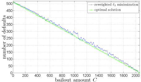
Fig. 1: Illustration of the algorithm for Problem II.

We test the algorithm on a network for which we know the optimal solution. We use a full binary tree with 10 levels and $N=2^{10}-1$ nodes: levels 0 and 9 correspond to the root and the leaves, respectively. Every node at level $s<9$ owes $\$2^{10-s}$ to each of its two creditors (children). We set ${\bf e}={\bf 0}$.

If $C=0$, then all 511 non-leaf nodes are in default, and the 512 leaves are not in default. In aggregate, the nodes at any level $s<9$ owe $\$2048$ the nodes at level $s+1$. Therefore, if $C\geq\$2048$, then $N_{d}=0$ can be achieved by allocating the entire amount to the root node.

For $0<C<2048$, we first observe that if $C=2^{11-s}$ for some integer $s$, then the optimal solution is to allocate the entire amount to a node at level $s$. This would prevent the defaults of this node and all its non-leaf descendants, leading to $511-(2^{9-s}-1)$ defaults. If $C$ is not a power of two, we can represent it as a sum of powers of two and apply the same argument recursively, to yield the following optimal number of defaults:

$$N_{d}=\displaystyle 511-\sum_{u=3}^{U}b(u)\cdot(2^{u-2}-1),$$

where $b(u)$ is the $u$-th bit in the binary representation of $C$ (right to left) and $U$ is the number of bits. The green line in Fig. 1 is a plot of the minimum number of defaults as a function of $C$. The blue line is the solution calculated by our reweighted $\ell_{1}$-minimization algorithm with $K=1000$, $\epsilon=0.001$ and $\delta=0.001$. The algorithm was run using six different initializations: five random ones and $\bf w^{(0)}=1$. Among the six solutions, the one with the smallest number of defaults was selected. As evident from Fig. 1, the results are very close to the optimal for the entire range of $C$.

References

- [1] E.J. Candès, M.B. Wakin, and S.P. Boyd. Enhancing sparsity by reweighted minimization. Journal of Fourier Analysis and Applications, 14(5-6):877–905, 2008.
- [2] L. Eisenberg and T.H. Noe. Systemic risk in financial systems. Management Science, 47(2):236–249, February 2001.