Moduli Stabilization in a de Sitter Compactification Model

Abstract:

We discuss the moduli stabilization in a de Sitter compactification model obtained coupling $D$-dimensional gravity to scalar and gauge fields. This class of models is characterized by two moduli: one related to the volume of the internal space, the other to the warp factor. While the volume modulus can be fixed by appropriately tuning the gauge field strength, curvature of the internal space, and cosmological constant, the same mechanism does not work for the warp modulus. In this paper we discuss a stabilization mechanism based on quantum effects and show that both moduli can be efficiently stabilized.

1 Introduction

The recent discovery of dark energy demands a mechanism setting the cosmological constant to a value that is nonzero but hierarchically small compared to the Planck scale. At the same time, a lot of recent observational data, in particular those of the cosmic microwave background, support the basic predictions of inflationary scenarios. A theoretical framework that may be able to provide a consistent description of the universe, undergoing inflation at early times and dominated by dark energy at the present day, is offered by string theory. In general, string theory requires the presence of extra dimensions that have to be stabilized at some appropriate scale to obtain a viable cosmological model. The lack of such a mechanism is often called the moduli stabilization problem. The stabilization of moduli is deeply connected with the realization of above accelerating phases in the cosmic history, and plays an important role in the construction of higher-dimensional cosmological models (See e.g., [1, 2, 3, 4]).

While the problem of moduli stabilization has been discussed at length for the case of Kaluza-Klein compactifications, its analysis for warped compactifications remains much less extensive [5, 6, 7]. In fact, the case of warped compactifications is an interesting set-up to consider since, due to the warping and external directions, multiple scalar moduli may appear and mix in a non-trivial way, affecting, in principle, each other’s dynamics. The present paper aims at discussing an example of this sort.

Specifically, we will consider gravity coupled to a scalar dilaton and a form field strength propagating on the background of a higher-dimensional warped geometry of the form

$$ds^{2} = {\rm e}^{2A(y)}\left[q_{\mu\nu}({\rm U})du^{\mu}du^{\nu}+dy^{2}+{\gamma}_{ab}({\rm Z})dz^{a}dz^{b}\right],$$ (1)

where $ds^{2}({\rm U})=q_{\mu\nu}({\rm U})du^{\mu}du^{\nu}$ and $ds^{2}({\rm Z})={\gamma}_{ab}({\rm Z})dz^{a}dz^{b}$ represent, respectively, the line elements of two maximally symmetric, non-singular manifolds U and Z, and $y$ is the direction of warping. The coordinates $u^{\mu}$ and $z^{a}$ parametrize, respectively, the manifolds ${\rm U}$ and ${\rm Z}$. Z is assumed to be compact. The dimensionalities of U and Z are, respectively, $n$ and $D-n-1$. Solutions of the above type have been discussed in Ref. [8] and will be briefly recalled here for the convenience of the reader.

The class of models that will be considered in this work is described, in the Einstein frame, by the following action

$$S=\frac{1}{2\kappa^{2}}\int\Big{[}\left\{R-2{\rm e}^{-\alpha\phi/(p-1)}\Lambda\right\}\ast{\bf 1}-\frac{1}{2}d\phi\wedge\ast d\phi-\frac{1}{2\cdot p!}{\rm e}^{\alpha\phi}F\wedge\ast F\Big{]},$$ (2)

where $\kappa^{2}$ is the $D$-dimensional gravitational constant, $\ast$ is the Hodge operator in $D$-dimensions, $\phi$ is a scalar field, $F$ is a $p$-form field strength, and $\Lambda$ and $\alpha$ are constants.

The equations of motion follow directly from the above action. The $p$-form field strength is taken to be proportional to the volume form of ${\rm Z}$,

$$\Omega({\rm Z})=\sqrt{\gamma}dz^{1}\wedge\cdots\wedge dz^{p}\,,$$

that is

$$F=f\,\Omega({\rm Z})\,,~{}~{}~{}~{}p=D-n-1\,,$$ (3)

with $f$ constant and $\gamma$ denoting the determinant of the metric $\gamma_{ab}$. The choice (3) guarantees that both the Bianchi identities and the equation of motion for the gauge field are automatically satisfied.

The ansatz for the scalar field $\phi$ is

$$\phi=\frac{2}{\alpha}(p-1)A(y)\,,$$ (4)

leading to the following equation:

$$A^{\prime\prime}+(D-2)\left(A^{\prime}\right)^{2}-\frac{\alpha^{2}\hat{\Lambda}}{p-1}=0\,,$$ (5)

where $\hat{\Lambda}=-\frac{\Lambda}{p-1}+\frac{f^{2}}{4}$ and ^′ denotes the ordinary derivative with respect to the coordinate $y$. Finally, using the metric ansatz (1), Einstein equations can be expressed as

$$R_{\mu\nu}({\rm U})-\beta\hat{\Lambda}q_{\mu\nu}({\rm U})=0\,,$$ (6a)

$$A^{\prime\prime}+\frac{2(p-1)^{2}}{(D-1)\alpha^{2}}\left(A^{\prime}\right)^{2}-2\frac{(p-1)}{(D-1)}\hat{\Lambda}=0\,,$$ (6b)

$$R_{ab}({\rm Z})-\left(\beta\hat{\Lambda}+\frac{f^{2}}{2}\right)\gamma_{ab}({\rm Z})=0\,,$$ (6c)

where $R_{\mu\nu}({\rm U})$ and $R_{ab}({\rm Z})$ are the Ricci tensors of the metrics $q_{\mu\nu}$ and $\gamma_{ab}$, respectively, and the constant $\beta$ is defined by

$$\beta=\frac{\alpha^{2}}{p-1}-\frac{2(p-1)}{D-2}\,.$$ (7)

Off-diagonal components of the Einstein equations are automatically satisfied by our ansatz. Eqs.(5) and (6b) can be simultaneously solved as

$$A(y)=\ell\left(y-y_{0}\right)\,,$$ (8)

with $v_{0}$ constant and $\ell$ given by

$$\ell=\pm\,\alpha\,\sqrt{\frac{\hat{\Lambda}}{(p-1)(D-2)}}\,.$$ (9)

Notice that the above solution is only compatible with the condition $\alpha^{2}\neq 2(p-1)^{2}/(D-2)$. Choosing $\alpha$ such that $\beta>0$ ensures that both ${\rm U}$ and ${\rm Z}$ are positively curved, as it is clear from an inspection of Eq. (6c). This corresponds to taking

$$\alpha>\sqrt{\frac{2}{D-2}}\,(p-1)\,,~{}~{}~{}~{}~{}~{}\alpha<-\sqrt{\frac{2}{D-2}}\,(p-1)\,.$$ (10)

In this case, the field equations lead to the following solution for the $D$-dimensional metric

$$ds^{2}={\rm e}^{2\ell(y-y_{0})}\left[q_{\mu\nu}^{({\rm dS})}du^{\mu}du^{\nu}+dy^{2}+\gamma_{ab}({\rm Z})dz^{a}dz^{b}\right]\,,$$ (11)

where $q_{\mu\nu}^{({\rm dS})}$ represents the metric of de Sitter space with expansion rate $H^{2}={\beta\hat{\Lambda}\over n-1}$ as it follows from Eq. (6a).

Details will be given later, here we simply mention that starting from the above background solution, an effective theory can be directly derived by compactifying the ${\rm Z}$ space. In the simplest construction, the effective theory contains two unstabilized moduli: one related to the volume of the internal space ${\rm Z}$, and another to the warp factor. As we will see, simultaneous stabilization of both moduli may not be achieved by means of the same mechanism. For instance, appropriately tuning the gauge field strength, curvature of the spherical internal space, and cosmological constant may help to achieve stabilization of the volume modulus but not of the warp factor [8, 9].

A different stabilization mechanism can be constructed by using quantum effects. In this case, if the volume modulus is stabilized due to the presence of a gauge field strength, its quantum fluctuation as well as those of the modulus associated to the warp factor may both contribute to stabilize or destabilize the background geometry. After flux stabilization, the volume modulus fluctuates around the minima of the effective potential and its contribution can be computed in a straightforward manner. On the other hand, at tree level, the dynamics of the warp modulus is controlled by a runaway type of potential, and its quantum fluctuations should be analyzed with care. In the following, we will adopt a self-consistent approach and require that any acceptable minima of the effective potential must occur where the potential is sufficiently flat.

An important point to remark is related to the value of the scalar potential after stabilization. In principle, once quantum corrections are included, the scalar potential of the system may occur at a positive, vanishing or negative value, resulting in a de Sitter, Minkowski or anti de Sitter geometry. In this case, we may expect that additional corrections to the potential, for example due to finite temperature effects, may produce a further shift up-lifting its minima from anti-de Sitter to Minkowski or de Sitter, or, at very high temperature, pushing the system into an unstabilized phase.

The paper is organized as follows. In Sec. 2, we will present the model in detail and construct the effective theory tuning the field strength to achieve stabilization of the volume modulus at the classical level. The main part of the paper is devoted to discuss how quantum effects from moduli contribute to the effective potential at one-loop. We will adopt the background field method and path integrals to perform the computation and use a zeta function regularization. Specifically, Sec. 3 deals with the contribution from the warp modulus to see whether its quantum fluctuations may provide any stabilization. In fact, due to the runaway behavior of the potential, as we have already mentioned, the minima (if any) generated by quantum fluctuations must be in a region where perturbation theory can be trusted. This self-consistency requirement is then verified a posteriori. After presenting the machinery we will perform the computation using an approach based on contour integral techniques similar to that described in Refs. [10, 11, 12, 13] (Related work is that of Refs. [14, 15, 16, 17, 18]). This method is valid over the whole parameter space and serves as a general way to compute the one-loop effective potential. In a restricted range of the parameter space a slightly simplified approach based on the Schwinger-De Witt approximation can be adopted. This method uses directly the small-$t$ heat-kernel asymptotics and it applies only in a small region of the parameter space. Details of this second approach will be given in Appendix A where the validity of the Schwinger-De Witt approximation will also be discussed. Results using both method are consistent when applied to the same region of the parameter space. (In Appendix B we will show how finite temperature corrections may produce transitions between different minima uplifting the vacuum. These effects are studied by means of the standard Matsubara formalism.) We will show that quantum corrections from the warp modulus can provide stabilization and lead to a de Sitter, Minkowski or anti de Sitter minimum. Unfortunately, the region of the parameter space for the moduli-stabilization consistent with the semi-classical approximation is only marginal. In Sec. 4 we add the contribution to the potential from from quantum fluctuations of the volume modulus again using an approach based on contour integrals and show that this may provide an efficient framework for stabilization. This seems rather natural, since after flux compactification the size of the internal space generically becomes of order of the Planck length. In this case, it is not possible to ignore quantum fluctuations of the volume modulus, even though the volume is already stabilized. These contributions to the one-loop effective potential may stabilize the warped direction and naturally realize a de Sitter, Minkowski or anti de Sitter minimum depending on the values of the parameters and of the renormalization scale. Our conclusions close the paper.

2 The effective theory with field strengths

The effective theory will be constructed in this section by promoting the warp factor and the size of the external manifold ${\rm Z}$ to scalar degrees of freedom. To do so, we express the metric (1) in the following way:

$$ds^{2}={\rm e}^{2\bar{A}(u_{\mu},y)}\left[q_{\mu\nu}({\rm U})du^{\mu}du^{\nu}+dy^{2}+{\rm e}^{2\bar{\psi}(u_{\mu},y)}\gamma_{ab}({\rm Z})dz^{a}dz^{b}\right]\,.$$ (12)

The background solution discussed in the previous section corresponds to the above metric once $\bar{A}=A(y)$ as given in (8) and $\bar{\psi}=constant$.

Using (3), (4) and (12) in the $(n+1)$-dimensional action (2), after using the equation of motion for the background solution, we get

$$S = \frac{1}{2\tilde{\kappa}^{2}}\int_{\bar{{\rm M}}}\left[\left\{R(\bar{{\rm M}})-V\left(\bar{A},~{}\bar{\psi}\right)\right\}\ast_{\bar{{\rm M}}}{\bf 1}_{\bar{{\rm M}}}-\frac{1}{2}d\bar{A}\wedge\ast_{\bar{{\rm M}}}d\bar{A}\right.$$ (13)

$$\left.-\frac{1}{2}\frac{c_{2}}{\sqrt{c_{1}c_{3}}}d\bar{A}\wedge\ast_{\bar{{\rm M}}}d\bar{\psi}-\frac{1}{2}d\bar{\psi}\wedge\ast_{\bar{{\rm M}}}d\bar{\psi}\right],$$

where $R(\bar{{\rm M}})$ is the Ricci scalar corresponding to the conformally transformed metric $w_{PQ}(\bar{{\rm M}})dv^{P}dv^{Q}={\rm e}^{2[(D-2)A+p\psi]/(n-1)}\left(q_{\mu\nu}({\rm U})du^{\mu}du^{\nu}+dy^{2}\right)$. The Hodge operator on $\bar{{\rm M}}$ space is defined as $\ast_{\bar{{\rm M}}}$ and $\tilde{\kappa}$ is given by $\tilde{\kappa}=V^{-1/2}\kappa$ with the volume of the internal space ${\rm Z}$ given by

$$V\equiv\int_{{\rm Z}}\ast_{{\rm Z}}{\bf 1}_{{\rm Z}}\,.$$ (14)

In obtaining Eq. (13), we have dropped the surface terms coming from ${\triangle}_{\bar{{\rm M}}}A$, ${\triangle}_{\bar{{\rm M}}}\psi$, where ${\triangle}_{\bar{{\rm M}}}$ is the Laplace operator constructed from the metric $w_{PQ}(\bar{{\rm M}})$. The potential $V\left(\bar{A},~{}\bar{\psi}\right)$ is given by

$$V\left(\bar{A},\bar{\psi}\right) = U(\bar{A})W(\bar{\psi})~{},$$ (15)

where

$$U(\bar{A}) = \exp\left[-\frac{2(D-2)\bar{A}}{(n-1)\sqrt{c_{1}}}\right],$$ (16a)

$$W(\bar{\psi}) = 2\Lambda\exp\left\{-\frac{2p\bar{\psi}}{(n-1)\sqrt{c_{3}}}\right\}+\frac{f^{2}}{2}\exp\left\{-\frac{2np\bar{\psi}}{(n-1)\sqrt{c_{3}}}\right\}$$ (16b)

$$-p\lambda\exp\left\{-\frac{2(D-2)\bar{\psi}}{(n-1)\sqrt{c_{3}}}\right\}.$$

The fields $\bar{A}$, $\bar{\psi}$ have been rescaled according to

$$\bar{A}=\sqrt{c_{1}}A\,,~{}~{}~{}~{}~{}~{}\bar{\psi}=\sqrt{c_{3}}\psi\,,$$ (17)

with the constants $c_{i}~{}(i=1,2,3)$ defined by

$$c_{1} = 2\left[\frac{n}{n-1}(D-2)-2(D-1)\right](D-2)$$ (18a)

$$+2\left[n-1+\frac{2}{\alpha^{2}}(p-1)\right](p-1)+2p(D-1)\,,$$

$$c_{2} = \frac{4(D-2)p}{n-1}\,,$$ (18b)

$$c_{3} = 2p\left(\frac{n-1}{p}+1\right)\,.$$ (18c)

The absence of a stabilization mechanism for the modulus associated to the warp factor is clear from the form of the potential in Eq. (15). In the $\bar{A}$-direction the potential decays exponentially causing the modulus $\bar{A}$ to suffer from a runaway behavior and the warped direction to expand forever. In the present set-up, classically, the warped direction cannot be stabilized. On the other hand the vacuum expectation value of $\bar{\psi}$ can be fixed by appropriately tuning the gauge field (see Fig. 1). The potential energy at the minimum is equivalent to the $(n+1)$-dimensional cosmological constant. Since the moduli potential energy eventually turns out to be positive or negative, the $(n+1)$-dimensional background geometry becomes dS_n+1 or AdS_n+1 spacetime.

Figure 1: The figure illustrates the behavior of the potential $W(\bar{\psi})$. The left panel displays the potential for vanishing gauge field, $f=0$, and for several values of the constant $\lambda$ (with $\Lambda$ normalized to unity). The right panel shows the potential for several choices of $f$ (with the values set as indicated in the figure). Dimensionality parameters are chosen as follows: $D=10$, $p=6$ and $n=3$.

In the following, we will assume that the modulus $\bar{\psi}$ is fixed at $\bar{\psi}=\bar{\psi}_{0}$ by tuning the gauge field flux. This does not affect the dynamics of the other modulus $\bar{A}$, whose stabilization will be considered in the next section.

As far as quantum corrections from the $p$-form field are concerned, these only produce a small in the constant $f$, therefore not affecting the classical stabilization of the modululs $\psi$. As it can be seen from Eqts. (1.6) such corrections: 1) will not spoil the classical background solution, 2) and will not be able to stabilize the potential for the other modulus $A$. The situation may be different, if one wished to introduce additional moduli by perturbing along other directions the classical background solution.

3 Quantum effects from the modulus $A$

In this section, we will discuss the possibility of stabilizing the modulus degree of freedom associated with the warp factor in the lower-dimensional effective theory described in Sec. 2. We will adopt the background field method and the path integral approach to compute the effective potential at one-loop for the moduli-field and deal with the divergences using zeta-function regularization.

Let us consider the $(n+1)$-dimensional scalar sector of the action (13)

$$I_{\bar{A}}\left[\bar{\psi}_{0},~{}\bar{A}(u_{\mu},y)\right]=-\frac{1}{2\tilde{\kappa}^{2}}\int_{\bar{{\rm M}}}\left[\frac{1}{2}d\bar{A}\wedge\ast_{\bar{{\rm M}}}d\bar{A}+V\left(\bar{A},~{}\bar{\psi}_{0}\right)\ast_{\bar{{\rm M}}}{\bf 1}_{\bar{{\rm M}}}\right],$$ (19)

and expand the field $\bar{A}$ around its classical vacuum expectation value, $\bar{A}_{0}$ given by (8),

$$\bar{A}(u_{\mu},y)=\bar{A}_{0}+a~{},$$ (20)

with $a$ representing the quantum fluctuation. Expanding the action up to second order

$$S=\frac{1}{2\tilde{\kappa}^{2}}\int_{\bar{{\rm M}}}\left[\left\{R(\bar{{\rm M}})-V\left(a,~{}\bar{A}_{0},~{}\bar{\psi}_{0}\right)\right\}\ast_{\bar{{\rm M}}}{\bf 1}_{\bar{{\rm M}}}-\frac{1}{2}da\wedge\ast_{\bar{{\rm M}}}da\right],$$ (21)

where linear terms in $a(u_{\mu},y)$ have disappeared owing to the classical equations of motion and the potential $V\left(a,~{}\bar{A}_{0},~{}\bar{\psi}_{0}\right)$ is given by

$$V\left(a,~{}\bar{A}_{0},~{}\bar{\psi}_{0}\right)=U(\bar{A}_{0})W(\bar{\psi}_{0})\left[1+\frac{2(D-2)^{2}}{(n-1)^{2}c_{1}}a^{2}\right]+O(a^{3}).$$ (22)

After varying the action with respect to $a$, we obtain the field equations for the fluctuation

$$\left({\triangle}_{\bar{{\rm M}}}-M^{2}_{a}\right)a=0\,,$$ (23)

where $M^{2}_{a}$ is given by

$$M^{2}_{a}=\frac{2(D-2)^{2}}{(n-1)^{2}c_{1}}U(\bar{A}_{0})W(\bar{\psi}_{0})\,.$$ (24)

Using path integrals we can express the amplitude as

$$Z=\int{\cal D}[a]\exp{\left(iI_{\bar{A}}[\bar{\psi}_{0},~{}\bar{A}]\right)},$$ (25)

where ${\cal D}[a]$ is a measure on the functional space of scalar fields $a(u_{\mu},y)$, and $I_{\bar{A}}[\bar{\psi}_{0},~{}\bar{A}]$ is given by (19). At one-loop, it is sufficient to compute the above path integral with the action expanded up to second order around its classical background value,

$$I_{\bar{A}}\left[\bar{\psi}_{0},~{}\bar{A}(u_{\mu},y)\right]=I_{\rm c}\left[\bar{\psi}_{0},~{}\bar{A}_{0}\right]+I_{\rm q}\left[\bar{\psi}_{0},~{}\bar{A}_{0},~{}a\right]+O\left(a^{3}\right),$$ (26)

where $\bar{A}(u_{\mu},y)$ is given by (20) and linear terms in $a$ have disappeared due to the classical equations of motion. Using the above expression, the path integral (25) becomes

$$\ln Z=iI_{\rm c}\left[\bar{\psi}_{0},~{}\bar{A}_{0}\right]+\ln\left\{\int{\cal D}\left[a\right]\exp{\left(iI_{\rm q}\left[\bar{\psi}_{0},~{}\bar{A}_{0},~{}a\right]\right)}\right\}.$$ (27)

The above integral is ill-defined because the operators in Eq. (27) are unbounded from below in the dS_n+1 spacetime with Lorentz signature. In order to correct this pathology, we proceed in the usual way and by performing a Wick rotation re-express (27) in the Euclidean form,

$$\ln Z=-I_{\rm cE}[\bar{\psi}_{0},~{}\bar{A}_{0}]+\ln\left\{\int{\cal D}[a]\exp{\left(-I_{\rm qE}[\bar{\psi}_{0},~{}\bar{A}_{0},~{}a]\right)}\right\},$$ (28)

where $I_{\rm qE}$ is the Euclidean action expressed by

$$I_{\rm qE}[\bar{\psi}_{0},~{}\bar{A}_{0},~{}a]=\frac{1}{4\tilde{\kappa}^{2}}\int_{\bar{{\rm M}}}a\left[-d\ast_{\bar{{\rm M}}}d+M^{2}_{a}\ast_{\bar{{\rm M}}}{\bf 1}_{\bar{{\rm M}}}\right]a\,.$$ (29)

Here we have integrated by parts over the kinetic term.

The one-loop quantum effective potential $V_{\rm q}$ is defined according to the relation

$$\exp\left[-\int_{\bar{{\rm M}}}V_{\rm q}(\bar{\psi}_{0},~{}\bar{A}_{0})\ast_{\bar{{\rm M}}}{\bf 1}_{\bar{{\rm M}}}\right] = \int{\cal D}\left[a\right]\exp\left(-I_{\rm qE}[\bar{\psi}_{0},~{}\bar{A}_{0},~{}a]\right)$$ (30)

$$= \left[\det\mu^{-2}\left({\triangle}_{\bar{{\rm M}}}-M^{2}_{a}\right)\right]^{-\frac{1}{2}},$$

where ${\triangle}_{\bar{{\rm M}}}$ denotes the Laplace operator on $(n+1)$-dimensional de Sitter spacetime, and $\mu$ is a normalization constant with dimension of mass. Defining

$$\exp\left[-\int_{\bar{{\rm M}}}V_{\rm q}(\bar{\psi}_{0},~{}\bar{A}_{0})\ast_{\bar{{\rm M}}}{\bf 1}_{\bar{{\rm M}}}\right]=\exp\left[-\Omega_{\rm vol}V_{\rm q}(\bar{\psi}_{0},~{}\bar{A}_{0})\right],$$ (31)

with $\Omega_{\rm vol}$ being the volume of $(n+1)$-dimensional de Sitter spacetime, we obtain the following expression

$$V_{\rm eff}(\bar{\psi}_{0},~{}\bar{A}_{0})=V_{0}(\bar{\psi}_{0},~{}\bar{A}_{0})+\frac{1}{2\Omega_{\rm vol}}\ln\det\left[\mu^{-2}\left({\triangle}_{(\bar{{\rm M}})}-M^{2}_{a}\right)\right],$$ (32)

where the above functional determinant has to be evaluated on dS_n+1.

A natural way to proceed is to use zeta regularization techniques. Defining the following generalized zeta function

$$\zeta_{a}(s) \equiv \sum_{\lambda}\left(\lambda+M^{2}_{a}\right)^{-s},$$ (33)

where $\lambda$ are the eigenvalues of the Laplacian on dS_n+1, the effective potential (32) can be expressed as

$$V_{\rm eff}(\bar{\psi}_{0},~{}\bar{A}_{0})=V_{0}(\bar{\psi}_{0},~{}\bar{A}_{0})-\frac{1}{2\Omega_{\rm vol}}\left[{\zeta_{a}}^{\prime}(0)+2\zeta_{a}(0)\ln(\mu b)\right],$$ (34)

where $b$ is the radius of a $(n+1)$-dimensional sphere Sⁿ⁺¹. The task is then to find the analytically continued values of the zeta function and its derivative, $\zeta_{a}(0)$ and $\zeta_{a}^{~{}\prime}(0)$. The one-loop effective potential can be computed in a variety of ways. The most advantageous one is to use contour integral techniques, which will be done in the reminder of this section. However, to see the overall feature of the effective potential, the simplest way would be the ‘Schwinger-De Witt’ approximation, which will be performed in Appendix (A).

The $(n+1)$-dimensional de Sitter geometry, dS_n+1, is a $(n+1)$-dimensional manifold with constant curvature and has a unique Euclidean section Sⁿ⁺¹ with a radius $b$. We call the eigenvalues of the Laplacian on this spacetime $\lambda(\ell)$ and their degeneracy $d(\ell)$. These are explicitly given by [19]

$$d(\ell)=\frac{(2\ell+n)(\ell+n-1)!}{n!\,\ell!}\,,~{}~{}~{}~{}~{}\lambda(\ell)=\ell(\ell+n)\,.$$ (35)

Using the generalized zeta function Eq. (33) which can be explicitly re-expressed as

$$\zeta_{a}(s) \equiv \sum^{\infty}_{\ell=0}d(\ell)\left[\frac{\lambda(\ell)}{b^{2}}+M^{2}_{a}\right]^{-s},$$ (36)

the effective potential is given by Eq. (34). We will evaluate the analytically continued values of the zeta function (36) at $s=0$ referring to the method employed in Refs. [12, 13].

We perform the analytic continuation of the generalized zeta function to $s=0$ in the case of $n$ being an odd positive integer, since the value we are interested in is $n=3$. Then,

$$\zeta_{a}(s)=\sum^{\infty}_{\ell=0}\frac{(2\ell+n)(\ell+n-1)!}{n!\,\ell!}\left[\frac{\ell(\ell+n)}{b^{2}}+M^{2}_{a}\right]^{-s}\,.$$ (37)

Defining $N=(n+1)/2$ and using it as running variable $L=\ell+N$, we rewrite the above expression as

$$\zeta_{a}(s)=\sum^{\infty}_{L=N}D_{n}\left(L-\frac{1}{2}\right)\left[\frac{\Lambda_{n}\left(L-\frac{1}{2}\right)}{b^{2}}+M_{a}^{2}\right]^{-s},~{}$$ (38)

where we have defined

$$D_{n}\left(L-\frac{1}{2}\right) = \frac{2L-1}{(2N-1)!}\left[\left(L-\frac{1}{2}\right)^{2}-\left(N-\frac{3}{2}\right)^{2}\right]$$ (39a)

$$\times\cdots\times\left[\left(L-\frac{1}{2}\right)^{2}-\left(\frac{1}{2}\right)^{2}\right]\,,$$

$$\Lambda_{n}\left(L-\frac{1}{2}\right) = \left(L-\frac{1}{2}\right)^{2}-\left(N-\frac{1}{2}\right)^{2}\,.$$ (39b)

Using the residue theorem, we can replace the infinite mode sum over $L$ by complex integration, obtaining

$$Z_{\pm}(s)=-\frac{i}{2}\left(\frac{b}{B_{\rm N}}\right)^{2s}B_{\rm N}\int_{{\rm C}_{1}}dz\tan(B_{\rm N}\pi z)D_{n}(B_{\rm N}z)\left(z^{2}\mp 1\right)^{-s}\,,$$ (40)

where the contour ${\rm C}_{1}$ in the complex plane is showed in Fig. 2, and $B_{\rm N}^{2}$ is defined by

$$B_{\rm N}^{2} = \left(N-\frac{1}{2}\right)^{2}-\left(b\,M_{a}\right)^{2}\,,$$ (41)

(For a positive $B_{\rm N}^{2}$, $-\big{(}N-\frac{1}{2}\big{)}<bM_{a}<N-\frac{1}{2}$). For clarity, we will consider the two cases separately,

$$\zeta_{a}(s) = \left\{\begin{array}[]{cc}Z_{+}(s)&~{}{\rm if}~{}~{}B_{\rm N}^{2}>0\,,\\ Z_{-}(s)&~{}~{}{\rm if}~{}~{}B_{\rm N}^{2}<0\,.\end{array}\right.$$ (44)

Let us consider $Z_{+}(s)$ first. In order to avoid the branch points $z=\pm 1$, we may proceed by deforming the contour ${\rm C}_{1}$ into ${\rm C}_{2}$ as indicated in Fig. 2 (left panel), and express $Z_{+}$ as

$$Z_{+}(s) = \left(\frac{b}{B_{\rm N}}\right)^{2s}B_{\rm N}\left[\frac{i}{2}\left({\rm e}^{-i\pi s}+{\rm e}^{i\pi s}\right)\int^{\infty}_{0}dx\,D_{n}(iB_{\rm N}x)\left(x^{2}+1\right)^{-s}\tanh(B_{\rm N}\pi x)\right.$$ (45)

$$-\frac{i}{2}\,{\rm e}^{i\pi s}\int^{1}_{0}dx\>\tan\left\{B_{\rm N}\pi(x-i\epsilon)\right\}D_{n}(B_{\rm N}x)\left(1-x^{2}\right)^{-s}$$

$$\left.+\frac{i}{2}\,{\rm e}^{-i\pi s}\int^{1}_{0}dx\>\tan\left\{B_{\rm N}\pi(x+i\epsilon)\right\}D_{n}(B_{\rm N}x)\left(1-x^{2}\right)^{-s}\right]\,,$$

where $D_{n}(iB_{\rm N}x)$ defines the following polynomial with coefficients $r_{Nk}$

$$D_{n}(iB_{\rm N}x) = i(-1)^{N-1}\frac{2B_{\rm N}x}{(2N-1)!}\left[\left(B_{\rm N}x\right)^{2}+\left(N-\frac{3}{2}\right)^{2}\right]\cdots\left[\left(B_{\rm N}x\right)^{2}+\left(\frac{1}{2}\right)^{2}\right]$$ (46)

$$\equiv i(-1)^{N-1}\sum^{N-1}_{k=0}\;r_{Nk}\;\left(B_{\rm N}x\right)^{2k+1}\,.$$

The first term in Eq. (45) comes from the integral along the imaginary axis. The second and third terms in Eq. (45) are the contributions from the contour along the cut on the real axis. Using in the first term of (45) the following relation

$$\tanh(B_{\rm N}\pi x)=1-\frac{2}{{\rm e}^{2B_{\rm N}\pi x}+1}\,,$$ (47)

we arrive at

$$Z_{+}(s) = -\left(\frac{b}{B_{\rm N}}\right)^{2s}\left[\cos(\pi s)\frac{1}{\Gamma(s)}(-1)^{N-1}\sum^{N-1}_{k=0}r_{Nk}\left(B_{\rm N}\right)^{2k+2}\Gamma(k+1)\Gamma(s-k-1)\right.$$ (48)

$$+i\,B_{\rm N}\,\cos(\pi s)\int^{\infty}_{0}dx\,D_{n}(iB_{\rm N}x)\left(x^{2}+1\right)^{-s}\frac{2}{{\rm e}^{2B_{\rm N}\pi x}+1}$$

$$\left.+B_{\rm N}\sin(\pi s)\int^{1}_{0}dxD_{n}(B_{\rm N}x)\left(1-x^{2}\right)^{-s}\tan(B_{\rm N}\pi x)\right]\,.$$

Next, we consider the function $Z_{-}(s)$. This time, the branch points in the integrand are on the imaginary axis at $z=\pm i$. Therefore we deform the contour as indicated in Fig. 2 (right panel) and obtain

$$Z_{-}(s) = i\,\left(\frac{b}{|B_{\rm N}|}\right)^{2s}|B_{\rm N}|\int^{\infty}_{0}dx\,D_{n}(i|B_{\rm N}|x)\tanh(|B_{\rm N}|\pi x)\left(1-x^{2}\right)^{-s}$$ (49)

$$= \left(\frac{b}{|B_{\rm N}|}\right)^{2s}\left[(-1)^{N}\Gamma(-s+1)\sum^{N-1}_{p=0}r_{Np}\left(|B_{\rm N}|\right)^{2p+2}\left\{\frac{\Gamma(s-p-1)}{\Gamma(-p)}\cos(\pi s)\right.\right.$$

$$\left.+\frac{\Gamma(p+1)}{\Gamma(2+p-s)}\right\}-2i|B_{\rm N}|\left\{\cos(\pi s)\int^{\infty}_{1}dx\,D_{n}(i|B_{\rm N}|x)\frac{\left(x^{2}-1\right)^{-s}}{{\rm e}^{2|B_{\rm N}|\pi x}+1}\right.$$

$$\left.\left.+\int^{1}_{0}dx\,D_{n}(i|B_{\rm N}|x)\frac{\left(1-x^{2}\right)^{-s}}{{\rm e}^{2|B_{\rm N}|\pi x}+1}\right\}\right].$$

The above expressions, (48) and (49), can be easily expanded to get the analytically continued values $\zeta_{a}(0)$ and $\zeta^{\prime}_{a}(0)$.

Figure 2: The left panel shows the deformation of the contour ${\rm C}_{1}$ used in (3.22), replaced by the contour ${\rm C}_{2}$ that avoids the branch points at $z=\pm 1$. The right panel shows the deformation of the contour ${\rm C}_{1}$ used in (3.29), replaced by the contour ${\rm C}_{3}$ running parallel to the imaginary axis. The points $x_{k}$ are defined as: $x_{k}=B_{N}^{-1}\left(N+k+1/2\right)$ for (3.25) and $x_{k}=B_{\bar{N}}^{-1}\left(N+k-1\right)$ for (3.29).

In Figs. 3-4, for $n=3$, the behavior of $\bar{V}_{\rm eff}$ is numerically illustrated as a function of ${\bar{M}}_{a}^{2}$, with three parameters $\mu$ (or dimensionless $\mu b$), $\alpha$ and $b$. In the left panel of Fig. 3, the effective potential is shown for various $\mu b$ while fixing $b=0.4$ and $\alpha=1.0$, and in the right panel it is shown for various $\alpha$ while fixing $b=1.0$ and $\mu b=1.0$. On the other hand, in Fig. 4, it is shown for various $b$ while fixing $\alpha=1.0$, $\mu b=10$. For a decreasing $\mu b$ with fixed other parameters an AdS vacuum is lifted to de Sitter or Minkowski one. If $\alpha$ is below a critical value for a given set of other parameters, it is not possible to find a vacuum. Finally, for an increasing $b$ with fixed other parameters, the energy density of the de Sitter minimum decreases but the potential minimum eventually disappears before it becomes a Minkowski or AdS vacuum.

Similarly, if there is an AdS vacuum, as $b$ increases, the minima is lifted but eventually disappears before it becomes a de Sitter or Minkowski vacuum. The results of this subsection are confirmed by those obtained using the ‘Schwinger-De Witt’ approximation as described in appendix A.

Figure 3: The figures illustrate the effective potential ${V}_{\rm eff}$ for $\bar{M}_{a}^{2}$. In the left panel, $\mu b=3,4.5,6$ from the top (red), while fixing $\alpha=1$ and $b=0.4$. In the right panel, $\alpha=1.0-5.0$ from the top (red), while fixing $b=1.0$ and $\mu b=1.0$.

Figure 4: The figure illustrates ${V}_{\rm eff}$ for $\bar{M}_{a}^{2}$ for changing $b=0.8-1.2$ from the top (red) and fixing $\alpha=1.0$ and $\mu b=1.0$.

In the next section, we will consider the contribution to the potential of the quantum fluctuations of the volume modulus around the classical minimum $\bar{\psi}=\bar{\psi}_{0}$ determined by effects of the gauge flux and of the bulk cosmological constant.

4 Quantum contribution to the effective potential from the volume-modulus

In this section, we consider the case when the size of the internal space approaches the Planck length. In this case, quantum corrections can no longer be neglected. If the size of the internal space is larger than the Planck length, quantum effects can be analysed using the conventional loop expansion. In the opposite case, the loop expansion breaks down. Therefore, in the following, we assume that the radius of the extra dimensions is larger than the Planck length, which can provide a natural cut-off scale to the quantum field theory.

Even if stabilized by flux, the volume modulus $\bar{\psi}$ may still contribute to the dynamics of the moduli associated to the warp factor, $\bar{A}$ through the coupling of the quantum fluctuation of $\bar{\psi}$ to $\bar{A}$. In this section, using the contour integral method, we will compute the quantum contribution of the modulus $\psi$ at one-loop and discuss whether they can stabilize $\psi$. As for the quantum corrections of ${\bar{A}}$, we can expand $\bar{\psi}(u_{\mu},y)$ around a neighborhood of the local minimum of the potential $W(\bar{\psi})$,

$$\bar{\psi}(u_{\mu},y)=\bar{\psi}_{0}+\varphi(u_{\mu},y)\,,$$ (50)

where $\bar{\psi}_{0}$ is fixed owing to the gauge flux (see Sec. II B). The $(n+1)$-dimensional action (13) expanded up to quadratic order in $\varphi(u_{\mu},y)$ is

$$S=\frac{1}{2\tilde{\kappa}^{2}}\int_{\bar{{\rm M}}}\left[\left\{R(\bar{{\rm M}})-V\left(\bar{A},~{}\bar{\psi}_{0},~{}\varphi\right)\right\}\ast_{\bar{{\rm M}}}{\bf 1}_{\bar{{\rm M}}}-\frac{1}{2}d\varphi\wedge\ast_{\bar{{\rm M}}}d\varphi\right],$$ (51)

where the potential $V\left(\bar{A},~{}\bar{\psi}_{0},~{}\varphi\right)$ is given by

$$V\left(\bar{A},~{}\bar{\psi}_{0},~{}\varphi\right)=U(\bar{A})\left[W_{0}\left(\bar{\psi}_{0}\right)+W_{2}\left(\bar{\psi}_{0}\right)\varphi^{2}\right]+O(\varphi^{3})\,.$$ (52)

Note that linear terms disappear owing to the classical equation of motion and the second term explicitly denotes the coupling of the quantum fluctuations of the volume modulus $\varphi$ to the warp factor ${\bar{A}}$. In the above expression, the functions $W_{i}(\bar{\psi}_{0})~{}(i=0,2)$ are

$$W_{0}\left(\bar{\psi}_{0}\right) = 2\Lambda\varepsilon(p)+\frac{f^{2}}{2}\varepsilon(np)-p\lambda\,\varepsilon(D-2)\,,$$ (53a)

$$W_{2}\left(\bar{\psi}_{0}\right) = \frac{2}{(n-1)^{2}c_{3}}\left[2\Lambda p^{2}\,\varepsilon(p)+\frac{(npf)^{2}}{2}\varepsilon(np)-p\lambda(D-2)^{2}\varepsilon(D-2)\right],$$ (53b)

where we have defined

$$\varepsilon(x)={\rm e}^{-\frac{2x\bar{\psi}_{0}}{(n-1)\sqrt{c_{3}}}}~{}.$$ (54)

Varying the action with respect to $\varphi$ gives

$$\left({\triangle}_{\bar{{\rm M}}}-M^{2}_{\varphi}\right)\varphi=0\,,$$ (55)

with $M^{2}_{\varphi}$ is expressed by the relation

$$M^{2}_{\varphi}=U(\bar{A})\,W_{2}\left(\bar{\psi}_{0}\right)\,.$$ (56)

The calculation of the one-loop effective potential can be carried out using path integrals, and similar steps to those used in the previous section allow us to obtain

$$V_{\rm eff}(\bar{A},~{}\bar{\psi}_{0}) = U(\bar{A})W_{0}(\bar{\psi}_{0})+V_{\rm q}(\bar{A},~{}\bar{\psi}_{0})$$ (57)

$$= U({\bar{A}})W_{0}(\bar{\psi}_{0})+\frac{1}{2\Omega_{\rm vol}}\ln\det\left[\mu^{-2}\left({\triangle}_{\bar{{\rm M}}}-M^{2}_{\varphi}\right)\right],$$

where ${\triangle}_{\bar{{\rm M}}}$ denotes the Laplace operator on $(n+1)$-dimensional de Sitter spacetime, and $\mu$ is a normalization constant with dimension of mass. The $(n+1)$-dimensional de Sitter geometry, dS_n+1, is a $(n+1)$–dimensional manifold with constant curvature and has a unique Euclidean section Sⁿ⁺¹ with a radius $b$. In the following we will evaluate the potential by analytically continuing the generalized zeta function

$$\zeta_{\varphi}(s) \equiv \sum^{\infty}_{\ell=0}d(\ell)\left[\frac{\lambda(\ell)}{b^{2}}+M^{2}_{\varphi}\right]^{-s},$$ (58)

to $s\to 0$. The effective potential $V_{\rm eff}(\bar{A},~{}\bar{\psi}_{0})$ is then expressed as

$$V_{\rm eff}(\bar{A},~{}\bar{\psi}_{0})=U({\bar{A}})W_{0}(\bar{\psi}_{0})-\frac{1}{2\Omega_{\rm vol}}\left[{\zeta_{\varphi}}^{\prime}(0)+2\zeta_{\varphi}(0)\ln(\mu b)\right].$$ (59)

We will refer to the method employed in Refs. [12, 13]. The contribution of the quantum correction played an important role to the effective potential. We find that the quantum effective potential has a terms proportional to $M_{\varphi}$. The procedure is the same as that employed in Sec. III. C, except for the replacement of $M_{a}^{2}\to M_{\varphi}^{2}$.

As before, here we will focus on the case of $n$ odd and integer. Using the residue theorem, and defining

$$B_{\rm N}^{2} = \left(N-\frac{1}{2}\right)^{2}-\left(b\,M_{\varphi}\right)^{2}\,,$$ (60)

($B_{\rm N}^{2}$ is positive for $-\big{(}N-\frac{1}{2}\big{)}<bM_{\varphi}<N-\frac{1}{2}$), we will consider the two cases separately,

$$\zeta_{\varphi}(s) = \left\{\begin{array}[]{cc}Z_{+}(s)&~{}{\rm if}~{}~{}B_{\rm N}^{2}>0\,,\\ Z_{-}(s)&~{}~{}{\rm if}~{}~{}B_{\rm N}^{2}<0\,.\end{array}\right.$$ (63)

Following the same procedure as that in Sec. III C, we can finally reduce $Z_{+}(s)$ and $Z_{-}(s)$ to the same forms as Eqs. (48) and (49), respectively, with the replacement of the definition of $B_{N}^{2}$ as Eq. (60).

Figure 5: The figure in the left panel shows a typical configuration realizing a de Sitter minima after quantum stabilization. The small superposed figure represents the classical potential $W(\bar{\psi}_{0})$ for the volume modulus $\bar{\psi}$ after flux stabilization. In the left panel we have set: $\Lambda=1.2$, $\lambda=0.547$, $f=1.6$ and $\alpha=1$. The right hand panel shows how the minima of the potential depends on the value of $W(\bar{\psi}_{0})$. The top green curve corresponds to $W(\bar{\psi}_{0})=10^{-1}$ realizing a de Sitter vacuum, while the bottom purple curve corresponds to $W(\bar{\psi}_{0})=10^{-2}$ realizing an anti de Sitter vacuum. The red dotted line corresponds to $W(\bar{\psi}_{0})=0.053$ and realized a Minkowski vacuum.

Figure 6: The figure illustrates the dependence of the potential on the parameter $\alpha$. In the left panel we have set the parameters $\Lambda$, $\lambda$ and $f$ as in the previous figure in order to obtain, after flux stabilization, a positive minima, $W(\bar{\psi}_{0})=10^{-1}$. In the right panel we have reduced the flux to obtain $W(\bar{\psi}_{0})=10^{-4}$. In the first case (left panel), after quantum stabilization the minima is positive realizing a de sitter vacua, while in the right panel the minima is negative giving an anti de Sitter vacua. Decreasing the parameter $\alpha$ shifts the minima towards larger values, without changing the sign of the potential.

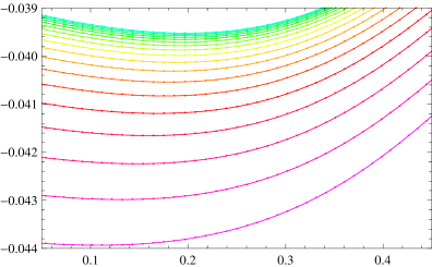
Figure 7: In this plot we show how the minima of the potential in the $\bar{A}$-direction shifts when the flux stabilizes the volume modulus to a negative value, generating an AdS vacua. The top curve refer to $W(\bar{\psi}_{0})=-10^{-4}$ while the bottom curve refers to $W(\bar{\psi}_{0})=-5\times 10^{-3}$. One may notice that for negative and decreasing values of $W(\bar{\psi}_{0})$ the minima of the potential accumulates around $V_{\rm min}\sim 0.0395$ for the present choice of parameters. For values of $W(\bar{\psi}_{0})$ below $5\times 10^{-3}$ the minima disappears.

The above expressions for the zeta functions can be directly used to obtain the one-loop effective potential. While explicit expressions can be obtained from formulae (48) and (49), here we follow a more expedite approach based on numerical approximation. Results are shown for the case of $n$ odd that we set $n=3$ and $B_{N}^{2}$ positive. Figs. 5-7 illustrate the effect of the one-loop corrections from quantum fluctuations of the volume modulus $\psi$ after flux stabilization. Depending on the value that the potential $W(\bar{\psi})$ attains at the minima, various possibilities can be realized. Fig. 5 shows a typical configuration that realizes a de Sitter minima, for positive $W(\bar{\psi}_{0})=10^{-1}$. The right panel of Fig. 5 shows how the potential depends on the value of $W(\bar{\psi}_{0})$ illustrating how, for increasing values of $W(\bar{\psi}_{0})$ the vacuum can be lifted from AdS to Minkowski or de Sitter. The quantum correction basically lifts the potential up without changing the shape too much around the minimum, which allows to uplifts the AdS minimum and make it a metastable de Sitter ground state. Fig. 6 depicts the dependence of the potential on the parameter $\alpha$, showing that a decrease in $\alpha$ tends to shift the minima towards larger values. Finally, for $W(\bar{\psi}_{0})$ negative, again an AdS vacua is realized and increasing $W(\bar{\psi}_{0})$ does not change the sign of the minima of the effective potential as long as $W(\bar{\psi}_{0})$ remains negative (see Fig. 7) and the potential tends to accumulate on the upper curve. For values of $0>W(\bar{\psi}_{0})$ below a certain critical value, it is not possible to achieve any minima when quantum effects are included.

The classical potential of $\bar{A}$ forces to decompactify the extra dimension while the combinations of matter and quantum correction produce a local minimum of the effective potential. Hence, the scale of the internal space ${\rm Z}$ is stabilized by balancing the 1-loop correction, gauge field strength wrapped around the internal space and the curvature term of the internal space with the cosmological constant. If we can have a negative potential minimum for a choice of the parameters, a dS_n+1 spacetime evolves into a AdS_n+1 when the modulus settles down to the potential minimum.

5 Discussions

In this paper, we have tackled the issue of the moduli stabilization in a class of higher dimensional models with two moduli. One ($\psi$) is related to the volume of the internal space, while the other ($A$) is related to the warped direction. These models provide interesting cosmological toy-models owing to the fact that it is possible to realize explicit exact de Sitter solutions.

In previous work (see Ref. [8]), the lower-dimensional effective theory has been derived, with the warped direction regarded as an external one and the warp factor as a modulus. Unfortunately, the lower-dimensional effective theory derived in Ref. [8] was problematic due to the runaway behavior of the potential. To address this problem here we have discussed a consistent mechanism of stabilization for the warp factor.

The example we have considered is simple enough, in the sense that only two moduli are included in the analysis. While the volume modulus can be fixed by appropriately tuning the gauge flux, the same mechanism cannot work for the modulus associated to the warp factor. Therefore, in the present paper, we have discussed whether quantum fluctuation from both moduli can lead to full stabilization. We have discussed this by using the background field method, path-integrals and zeta-function regularization, and showed that, quantum effects from both moduli may provide an efficient solution to the stabilization problem in the present model. In the presence of the 1-loop correction, the classical contributions from curvature and flux compete with quantum effects leading to a local minimum and showed that by tuning $\alpha$ and $\mu$, one can perturb the AdS vacua to produce dS vacua. The vacua will clearly only be metastable, since all of the sources of energy we have introduced vanish or become negative as $\bar{A}\rightarrow\infty$.

Appendix A ‘Schwinger-De Witt’ approximation

Here, we will provide a simpler way to compute the one-loop effective potential (34) directly using the Schwinger-De Witt expansion for the heat-kernel. This approach is valid in the region of parameter space for which the value of $M_{a}$ is large enough.

Using the Mellin transform, the zeta function can be expressed as

$$\zeta_{a}=\frac{1}{\Gamma(s)}\int^{\infty}_{0}dtt^{s-1}{\rm e}^{-(M^{2}_{a}+H^{2})t}\Theta(t)\,,$$ (64)

where $H:=b^{-1}$ is the Hubble scale of the de Sitter space and the function $\Theta(t)$ is the heat-kernel defined as

$$\Theta(t)=\sum_{\lambda}{\rm e}^{-(\lambda-H^{2})t}\,.$$ (65)

If the value of the mass $M_{a}$ is large enough, then the exponential in the integral above suppresses the contribution coming from the large-$t$ part of the integration range, and a direct use of the small-$t$ expansion is possible. This procedure is analogous to the high temperature expansion of the effective action. After rescaling the integral (64) by $t\rightarrow H^{-2}\bar{t}$, it is straightforward to realize that the exponential suppression becomes substantial when $M_{a}^{2}H^{-2}$ becomes large enough. Using (24), it is straightforward to see that choosing $\alpha\sim O(1)$ and tuning the gauge flux in such a way to obtain $W(\bar{\psi}_{0})\sim O(1)$, a small hierarchy between the Hubble parameter $H$ and the Planck mass ($H\sim 10^{-1}M_{\rm Pl}$) is sufficient to generate enough exponential suppression.

In this region we may approximate the integrand in (64) by using the Schwinger-De Witt expansion for $\Theta(t)$

$$\Theta(t)=\frac{1}{(4\pi t)^{(n+1)/2}}\sum_{k}\tilde{\theta}_{k}t^{k}\,,$$ (66)

where the coefficients $\tilde{\theta}_{k}$ are the heat-kernel coefficients [20, 21]. Explicit form for the coefficients can be found with little work and for the present case of de Sitter space with $\xi_{c}=\frac{3}{16}$ and $n=3$, these are

$${\tilde{\theta}}_{0}=\Omega_{\rm vol},~{}~{}{\tilde{\theta}}_{1}=-\Omega_{\rm vol}\left(\frac{1}{4}H^{2}\right),~{}~{}{\tilde{\theta}}_{2}=-\Omega_{\rm vol}\left(\frac{17}{480}H^{4}\right),~{}~{}{\tilde{\theta}}_{3}=-\Omega_{\rm vol}\left(\frac{457}{40320}H^{6}\right),$$ (67)

where ${\Omega}_{\rm vol}$ is defined by

$${\Omega}_{\rm vol}=\int d^{n+1}x\sqrt{g}\,.$$ (68)

A direct computation gives for the one-loop effective potential for $D=10$ and $n=3$ the following expression

$$\bar{V}_{\rm eff}(M_{a})=V_{0}+V_{\rm q}(M_{a})$$

$$~{}~{}~{}=\frac{8\alpha^{2}+25}{32\alpha^{2}}\bar{M}_{a}^{2}-\frac{1}{32\pi^{2}}\left[\frac{3}{4}\left(\bar{M}_{a}^{2}+2\bar{H}^{2}\right)^{2}\right.$$

$$\left.~{}~{}~{}~{}~{}+\left\{\frac{1}{2}\left(\bar{M}_{a}^{2}+2\bar{H}^{2}\right)^{2}-\frac{1}{15}\bar{H}^{4}\right\}\ln\left(\frac{\bar{\mu}^{2}}{\bar{M}_{a}^{2}+2\bar{H}^{2}}\right)-\frac{8}{315}\frac{\bar{H}^{6}}{\bar{M}_{a}^{2}+2\bar{H}^{2}}\right]\,,$$ (69)

where we have rescaled the various quantities according to

$$\bar{V}_{\rm eff} = V_{\rm eff}\,\tilde{\kappa}^{4}\,,~{}~{}~{}~{}~{}\bar{H}=H\tilde{\kappa}\,,$$

$$\bar{{M}_{a}} = M_{a}\tilde{\kappa}\,,~{}~{}~{}~{}~{}\bar{\mu}=\mu\tilde{\kappa}\,.$$

Eventual non-vanishing minima of the potential determine the mass of the field $a$:

$$0 = \Delta\bar{V}_{\rm eff}(\alpha,\bar{\mu},\bar{H},\bar{M}_{a}),$$ (70)

$$0 = \frac{\partial}{\partial\bar{M}_{a}^{2}}\Delta\bar{V}_{\rm eff}(\alpha,\bar{\mu},\bar{H},\bar{M}_{a}),$$ (71)

where we have normalized the potential according to

$$\Delta\bar{V}_{\rm eff}(\alpha,\bar{\mu},\bar{H},\bar{M}_{a}) := \bar{V}_{\rm eff}-3{\bar{H}}^{2}.$$ (72)

For a given set of $(\alpha,\bar{\mu},\bar{H})$, the solution for $\bar{M}_{a}$ leads to

$$V_{\rm eff}\simeq 3\tilde{\kappa}^{-4}\bar{H}^{2}\,.$$ (73)

Hence, for $H$ to be ${\bar{H}}\ll 1$ and $(\bar{M}_{a}/\bar{H})\gg 1$, then if one keeps ${\bar{\mu}}=O(1)$ fixed, the energy density at the minimum is much smaller than the Planck scale, which implies that the stabilization due to the quantum corrections is working consistently. In case of $D=10$ and $n=3$, the classical potential approaches a constant from above as $\alpha$ increases. For $\alpha$ tuned to be small but non-zero, the quantum correction no longer contribute to the effective potential. For modest values of $\alpha$, we will find numerically that there is a solution ${\bar{M}}_{a}\simeq 12$ for $\bar{\mu}\gtrsim 10$.

Approximate expressions for the minima of the potential can be found at leading order by expanding for $\bar{M}_{a}\gg\bar{H}$. In this regime the minima is determined by

$$\bar{M}_{a}^{2}\left[1+\ln\left(\frac{{\bar{\mu}}^{2}}{{\bar{M}}_{a}^{2}}\right)\right]=\frac{\pi^{2}}{\alpha^{2}}\left(25+8\alpha^{2}\right).$$ (74)

Assuming the renormalization scale to be of the same order as the mass, $\bar{\mu}\sim M_{a}$, we find

$$\bar{M}_{a}^{2}\simeq{\bar{\mu}}^{2}\left[1+\sqrt{1-\frac{\pi^{2}}{\alpha^{2}{\bar{\mu}}^{2}}(25+8\alpha^{2})}\right].$$ (75)

Higher order corrections do not change the qualitative features of the above result.

The value that the potential attains at the minima depends on the choice of the renormalization scale. Minimizing $\bar{V}_{\rm min}$ as a function of $\bar{\mu}$ allows to find a Minkowski vacua ($V_{\rm min}=0$) for

$${\bar{\mu}}_{\rm crit}^{2}\simeq\frac{4\pi^{2}}{3\alpha^{2}}(25+8\alpha^{2})=\frac{4}{3}\left[8\pi^{2}+\left(\frac{5\pi}{\alpha}\right)^{2}\right]>{\bar{\mu}}_{\rm min}^{2}\,,$$ (76)

where $\mu_{\rm min}$ is the minimum value of the renormalization scale for which a minima with positive vacuum energy exists. An AdS minimum ($V_{\rm min}<0$) is found for values of $\bar{\mu}$ in the range $\bar{\mu}>\bar{\mu}_{\rm crit}$, while a de Sitter minimum ($V_{\rm min}>0$) is obtained for values of $\bar{\mu}$ lying in the range $\bar{\mu}_{\rm min}<\bar{\mu}<\bar{\mu}_{\rm crit}$ and the expansion rate is given by

$$3\bar{H}^{2}\simeq-\frac{{\bar{\mu}}^{4}}{64\pi^{2}}\left[1-\frac{3\pi^{2}}{2\alpha^{2}{\bar{\mu}}^{2}}(25+8\alpha^{2})+\left\{1-\frac{\pi^{2}}{\alpha^{2}{\bar{\mu}}^{2}}(25+8\alpha^{2})\right\}^{\frac{3}{2}}\right].$$ (77)

The above arguments, although apply in a specific region of the parameter space of the model ($\bar{\mu}$ and $\alpha$) suggest that $a$ can be stabilized by quantum effects.

A more general computation of the one-loop effective potential valid in all regions of the parameter space was given in Sec. 3, which exhibits a behavior consistent with the results shown in this Appendix. The dependence of the potential on the energy scale suggests that the inclusion of finite temperature effects may lift the minima of the potential. Of course, these effects are not directly related to the mechanism of stabilization discussed in this paper, and clearly a proper inclusion of thermodynamic effects requires care, particularly if time dependence is taken into account. However, in the approximation that the time evolution of the moduli fields is adiabatic, it is possible to give an estimate of these effects using the standard Matsubara formalism. The argument becomes simpler if the scale of the Sⁿ is approximately constant, i.e. if we assume the adiabatic expansion in the direction of Sⁿ after compactification of the $(n+1)$-dimensional theory over S¹ to S${}^{n+1}=$S${}^{1}\times$Sⁿ with $H^{-1}$ being the radius of the spatial section Sⁿ. The computation of the potential at finite temperature carried out in Appendix B gives for $n=3$,

$$\bar{V}_{\rm eff} \simeq \frac{25+8\alpha^{2}}{32\alpha^{2}}\bar{M}_{a}^{2}-\frac{1}{32\pi^{2}}\left[\left(\bar{M}_{a}^{2}+\bar{H}^{2}\right)^{2}\left\{\frac{3}{4}-\frac{1}{2}\ln\left(\frac{\bar{M}_{a}^{2}+\bar{H}^{2}}{{\bar{\mu}}^{2}}\right)\right\}\right.$$ (78)

$$\left.+4\sum_{\ell=1}^{\infty}\left\{\frac{{\bar{\chi}}\left(\bar{M}_{a}^{2}+\bar{H}^{2}\right)}{\pi^{2}\ell^{2}}\right\}K_{-2}\left(2\pi\ell\sqrt{\frac{\bar{M}_{a}^{2}+\bar{H}^{2}}{\bar{\chi}}}\right)\right]\,,$$

where $\bar{\chi}=\tilde{\kappa}^{1/2}(2\pi T)^{2}$ and $T$ is the temperature. Details along with high- and low-temperature approximation are obtained in Appendix B. Here, we show the typical behavior of the potential in Fig. 8 where we have normalized its value by subtracting the vacuum energy contribution for $M_{a}=0$, which corresponds to the $A\to\infty$ limit.

Figure 8: The left panel illustrates the temperature dependence of the potential. The continuous-red curve is tuned to give a vanishing vacuum energy at the minima for $T=0$. Increasing the temperature shift the minima to a de Sitter vacuum (blue-dashed curve) and further increase of the temperature pushes the system into a symmetric high temperature phase (yellow-dotted curve). The right panel is illustrates the case in which the zero temperature minima is tuned to give a AdS vacuum (red-continuous curve), while blue-dotted curve gives a Minkowski minima and the yellow-dotted curve the de Sitter minima. (Left Panel) The parameters have been set to $\mu=100$ and $\alpha=7$. The curves correspond to the following values of the temperature: $T=0.1$ (bottom), $T=3.0$ (central), $T=4.0$ (top). (Right Panel) The parameters have been set to $\mu=120$, $\alpha=7.$ and the curves correspond to the following values of the temperature: $T=0.1$ (bottom), $T=3.0$ (central), $T=3.5$ (top).

Appendix B Finite temperature corrections

In this Appendix we present the computations of the finite temperature corrections to the effective potential. As mentioned in Appendix. A we assume that the time evolution of the modulus is adiabatic, allowing us to use the standard Matsubara formalism [22]. In this adiabatic regime, the scale of the Sⁿ, $H^{-1}$, is assumed to be approximately constant. The same formalism of Appendix A can be applied and the zeta function becomes

$$\zeta(s)=\sum_{\lambda,\,N}\left(\lambda+{M}_{a}^{2}+\chi N^{2}\right)^{-s}\,,$$ (79)

where $\lambda$ are the eigenvalues of the Laplace operator on the $n$-sphere, $N$ is integer, and $\chi$ is defined by $\chi=(2\pi T)^{2}$. Mellin-transforming the above expression and using the same heat-kernel scheme adopted in Appendix A, it takes simple steps to arrive at

$$\zeta(s) = \frac{1}{(4\pi)^{\frac{n}{2}}\Gamma(s)}\sqrt{\frac{\pi}{\chi}}\sum_{k}{\tilde{\theta}}_{k}\left[\left\{\left({M}_{a}^{2}+H^{2}\right)^{-k-s+\frac{n+1}{2}}\Gamma\left(s+k-\frac{n+1}{2}\right)\right\}\right.$$ (80)

$$\left.\!\!+4\sum_{\ell=1}^{\infty}\left(\frac{\sqrt{\chi({M}_{a}^{2}+H^{2})}}{\pi\ell}\right)^{-k-s+\frac{n+1}{2}}K_{k+s-\frac{n+1}{2}}\left(2\pi\ell\sqrt{\frac{{M}_{a}^{2}+H^{2}}{\chi}}\right)\right].$$

The important values $\zeta(0)$ and $\zeta^{\prime}(0)$ can be computed in a straightforward manner from the above expression, leading, for $n=3$, to

$$\bar{V}_{\rm eff} \simeq \frac{25+8\alpha^{2}}{32\alpha^{2}}\bar{M}_{a}^{2}-\frac{1}{32\pi^{2}}\left[\left(\bar{M}_{a}^{2}+\bar{H}^{2}\right)^{2}\left\{\frac{3}{4}-\frac{1}{2}\ln\left(\frac{\bar{M}_{a}^{2}+\bar{H}^{2}}{{\bar{\mu}}^{2}}\right)\right\}\right.$$ (81)

$$\left.+4\sum_{\ell=1}^{\infty}\left\{\frac{{\bar{\chi}}\left(\bar{M}_{a}^{2}+\bar{H}^{2}\right)}{\pi^{2}\ell^{2}}\right\}K_{-2}\left(2\pi\ell\sqrt{\frac{\bar{M}_{a}^{2}+\bar{H}^{2}}{\bar{\chi}}}\right)\right],$$

where we have used the definitions (A), and $\bar{\chi}=\tilde{\kappa}^{1/2}\chi$. The volume factor and the heat kernel coefficients are given by

$$\Omega_{\rm vol}=\frac{2\pi}{\sqrt{\chi}}\times H^{-3}\Omega_{3}\,,~{}~{}~{}~{}~{}{\tilde{\theta}}_{k}=\Omega_{3}{\tilde{\gamma}}_{k}H^{2k-3}\,.$$ (82)

Here $\Omega_{3}$ is the volume of S³, and ${\tilde{\gamma}}_{k}$ is given by ${\tilde{\gamma}}_{0}=1$ and ${\tilde{\gamma}}_{k}=0$ ($k=1,2,3$) for an S³.
Below we obtain the limiting behavior of (81) assuming $\bar{M}_{a}\gg\bar{H}$. At low temperature $\chi\rightarrow 0$, the modified Bessel functions decay exponentially as ${\rm e}^{-2\pi\ell\frac{\bar{M}_{a}}{\sqrt{\bar{\chi}}}}$, and the finite temperature corrections become small. Hence we can recover the result of Appendix A

$$\bar{V}_{\rm eff}\simeq\frac{25+8\alpha^{2}}{32\alpha^{2}}\bar{M}_{a}^{2}-\frac{1}{32\pi^{2}}\bar{M}_{a}^{4}\left[\frac{3}{4}-\frac{1}{2}\ln\left(\frac{\bar{M}_{a}^{2}}{{\bar{\mu}}^{2}}\right)\right].$$ (83)

The effective potential (83) has a minimum at

$$\bar{M}_{a}^{2}\simeq{\bar{\mu}}^{2}\left[1+\sqrt{1-\frac{1}{{\bar{\mu}}^{2}}\frac{\pi^{2}(8\alpha^{2}+25)}{\alpha^{2}}}\right],$$ (84)

where

$$\bar{V}_{\rm min}\simeq-\frac{{\bar{\mu}}^{4}}{64\pi^{2}}\left[1-\frac{3}{2{\bar{\mu}}^{2}}\frac{\pi^{2}(25+8\alpha^{2})}{\alpha^{2}}+\left\{1-\frac{1}{{\bar{\mu}}^{2}}\frac{\pi^{2}(25+8\alpha^{2})}{\alpha^{2}}\right\}^{\frac{3}{2}}\right].$$ (85)

A de Sitter minimum exists in the range

$$\frac{\pi^{2}(25+8\alpha^{2})}{\alpha^{2}}<{\bar{\mu}}^{2}<\frac{4}{3}\frac{\pi^{2}(25+8\alpha^{2})}{\alpha^{2}}.$$ (86)

At small temperature, expanding appropriately and then summing over $0<\ell\in\mathbb{N}$, we find

$$\bar{V}_{\rm eff} \simeq \frac{25+8\alpha^{2}}{32\alpha^{2}}\bar{M}_{a}^{2}-\frac{1}{32\pi^{2}}\bar{M}_{a}^{4}\left[\frac{3}{4}-\frac{1}{2}\ln\left(\frac{\bar{M}_{a}^{2}}{{\bar{\mu}}^{2}}\right)\right].$$ (87)

In the high temperature limit, we find

$$\bar{U}_{\rm eff} \equiv {\bar{V}}_{\rm eff}-\left(-\frac{{\bar{\chi}}^{2}}{1440\pi^{2}}\right)$$ (88)

$$\simeq\frac{25+8\alpha^{2}}{32\alpha^{2}}\bar{M}_{a}^{2}-\frac{1}{32\pi^{2}}\left[\frac{{\bar{\chi}}^{2}}{45}+\left(\bar{M}_{a}^{2}+\bar{H}^{2}\right)^{2}\left\{\frac{3}{4}-\frac{1}{2}\ln\left(\frac{\bar{M}_{a}^{2}+\bar{H}^{2}}{{\bar{\mu}}^{2}}\right)\right\}\right.$$

$$\left.+4\sum_{\ell=1}^{\infty}\left\{\frac{{\bar{\chi}}\left(\bar{M}_{a}^{2}+\bar{H}^{2}\right)}{\pi^{2}\ell^{2}}\right\}K_{-2}\left(2\pi\ell\sqrt{\frac{\bar{M}_{a}^{2}+\bar{H}^{2}}{\bar{\chi}}}\right)\right],$$

where we have summed over $\ell$ and proceeded with appropriate analytic continuation. The above expression is normalized by subtracting the vacuum energy contribution for $\bar{M}_{a}=0$. In the adiabatic approximation adopted, the effect of increasing the temperature is to uplift the minimum of the potential without changing its shape around the minimum.

References

[1]
P. G. O. Freund and M. A. Rubin,
“Dynamics of Dimensional Reduction,”
Phys. Lett. B 97, 233 (1980).
[2]
W. D. Goldberger and M. B. Wise,
“Modulus stabilization with bulk fields,”
Phys. Rev. Lett. 83, 4922 (1999)
[hep-ph/9907447].
[3]
S. M. Carroll, J. Geddes, M. B. Hoffman and R. M. Wald,
“Classical stabilization of homogeneous extra dimensions,”
Phys. Rev. D 66, 024036 (2002)
[hep-th/0110149].
[4]
B. R. Greene and J. Levin,
“Dark Energy and Stabilization of Extra Dimensions,”
JHEP 0711, 096 (2007)
[arXiv:0707.1062 [hep-th]].
[5]
H. Kodama and K. Uzawa,
“Moduli instability in warped compactifications of the type IIB
supergravity,”
JHEP 0507 (2005) 061
[arXiv:hep-th/0504193].
[6]
H. Kodama and K. Uzawa,
“Comments on the four-dimensional effective theory for warped
compactification,”
JHEP 0603 (2006) 053
[arXiv:hep-th/0512104].
[7]
H. Kodama and K. Uzawa,
“Moduli instability in warped compactification,”
hep-th/0601100.
[8]
M. Minamitsuji and K. Uzawa,
“Warped de Sitter compactifications,”
JHEP 1201 (2012) 142
[arXiv:1103.5326 [hep-th]].
[9]
M. Minamitsuji and K. Uzawa,
“Spectrum from the warped compactifications with the de Sitter universe,”
JHEP 1207, 154 (2012)
[arXiv:1103.5325 [hep-th]].
[10]
K. Uzawa,
“Dilaton stabilization in (A)dS spacetime with compactified dimensions,”
Prog. Theor. Phys. 110 (2003) 457
[arXiv:hep-th/0308170].
[11]
K. Uzawa and K. i. Maeda,
“Dilaton dynamics in (A)dSS5,”
Phys. Rev. D 68 (2003) 084017
[arXiv:hep-th/0308137].
[12]
K. Kikkawa, T. Kubota, S. Sawada and M. Yamasaki,
“Stability of selfconsistent dimensional reduction,”
Phys. Lett. B 144 (1984) 365.
[13]
K. Kikkawa, T. Kubota, S. Sawada and M. Yamasaki,
“Spontaneous compactification in generalized Candelas-Weinberg models,”
Nucl. Phys. B 260 (1985) 429.
[14]
A. Flachi, A. Knapman, W. Naylor and M. Sasaki,
“Zeta functions in brane world cosmology,”
Phys. Rev. D 70 (2004) 124011
[arXiv:hep-th/0410083].
[15]
A. Flachi, J. Garriga, O. Pujolas and T. Tanaka,
“Moduli stabilization in higher dimensional brane models,” JHEP 0308 (2003) 053 [hep-th/0302017].
[16]
A. Flachi and O. Pujolas,
“Quantum selfconsistency of AdS brane models,” Phys. Rev. D 68 (2003) 025023 [hep-th/0304040].
[17]
E. Elizalde, S. ’i. Nojiri, S. D. Odintsov and S. Ogushi,
“Casimir effect in de Sitter and anti-de Sitter brane worlds,”
Phys. Rev. D 67 (2003) 063515
[hep-th/0209242].
[18]
K. Milton and A. A. Saharian,
“Casimir densities for a spherical boundary in de Sitter spacetime,”
Phys. Rev. D 85 (2012) 064005
[arXiv:1109.1497 [hep-th]].
[19]
M. A. Rubin and C. R. Ordonez,
“Symmetric tensor eigen spectrum of the Laplacian on spheres,”
J. Math. Phys. 26 (1985) 65.
[20]
K. Kirsten, “Spectral Functions in Mathematics and Physics”,
Chapman and Hall/CRC (2001).
[21]
D. V. Vassilevich,
“Heat kernel expansion: User’s manual,”
Phys. Rept. 388 (2003) 279
[arXiv:hep-th/0306138].
[22]
J. I. Kapusta and C. Gale,
“Finite-temperature field theory: Principles and applications,”
Cambridge, UK: Univ. Pr. (2006).