The World’s Colonisation and Trade Routes Formation as Imitated by Slime Mould

Abstract

The plasmodium of Physarum polycephalum is renowned for spanning sources of nutrients with networks of protoplasmic tubes. The networks transport nutrients and metabolites across the plasmodium’s body. To imitate a hypothetical colonisation of the world and formation of major transportation routes we cut continents from agar plates arranged in Petri dishes or on the surface of a three-dimensional globe, represent positions of selected metropolitan areas with oat flakes and inoculate the plasmodium in one of the metropolitan areas. The plasmodium propagates towards the sources of nutrients, spans them with its network of protoplasmic tubes and even crosses bare substrate between the continents. From the laboratory experiments we derive weighted Physarum graphs, analyse their structure, compare them with the basic proximity graphs and generalised graphs derived from the Silk Road and the Asia Highway networks.

Keywords: biological transport networks, unconventional computing, slime mould

1 Introduction

Nature-inspired computing paradigms and experimental laboratory prototypes are demonstrated reasonable success in approximation of shortest, and often collision-free, paths between two given points in an Euclidean space or a graph. Examples include ant-based optimisation of communication networks [15], approximation of a shortest path in experimental reaction-diffusion chemical systems [1], gas-discharge analog systems [35], spatially extended crystallisation systems [5], fungi mycelia networks [22], and maze solving by Physarum polycephalum [29]. Amongst all explored so far experimental prototypes of path-computing devices slime mould P. polycephalum is the most user-friendly and easiest to cultivate and observe biological substrate. In its plasmodium stage, P. polycephalum spans scattered sources of nutrients with a network of protoplasmic tubes. Nakagaki and colleagues demonstrated that the plasmodium optimises its protoplasmic network to cover all sources of nutrients and to assure quick and fault-tolerant distribution of nutrients in the plasmodium’s body [28, 29, 30, 31]. There are experimental evidences [2] that in the course of the plasmodium’s foraging behaviour the protoplasmic network follows the Toussaint [43, 25, 21] hierarchy of proximity graphs however neither of the known proximity graphs is exactly matched by the protoplasmic networks [7].

The slime mould’s protoplasmic network is responsible for transportation of nutrients and metabolites, and intra-cellular communication. Therefore it is a matter of the natural scientific curiosity to compare the protoplasmic transport networks with man-made transport network. Two first comparisons were made by Adamatzky and Jones [3] — the slime mould imitation of the UK motorways, and Tero and colleagues [40] — the slime mould imitation of the Tokyo rail roads. These pioneering results were followed by a series of laboratory experiments on evaluation of motorway/highway networks in Mexico [4], Spain and Portugal [6], Brazil [8], Australia [9] and Canada [10]. These papers demonstrated that P. polycephalum approximates existing road networks up to some degree, especially with regards to the core spanning structure, but the slime mould also allows for a wide range of structural deviations in the transport networks and solutions are not always optimal or predictable. The shape of any particular country and the spatial configuration of major urban areas, represented by sources of nutrients, might substantially determine the resultant topology of the protoplasmic networks developed. In certain countries, the road network designs were influenced not only by logic but also by political, economic and somewhat idealogical decisions. Therefore, more experiments are required to provide a viable generalisation, to undertake a comparative analyses of slime mould transport networks constructed in different countries and to built a theory of P. polycephaum based road planning and associated urban development. In present paper we decided to undertake an experimental laboratory exercise on playing a hypothetical scenario of the colonisation of the World by large-scale amorphous substrate and formation of the world-wide transportation routes crossing countries and linking continents. The resultant protoplasmic networks were compared, at the abstract level of generalised graphs, with ancient road network — the Silk Road, and future road network — the Asian Highways.

2 Materials and methods

The plasmodium of P. polycephalum is cultivated in a plastic container, on paper kitchen towels moistened with still water, and fed with oat flakes. For experiments we use $220\times 220$ mm polystyrene square Petri dishes and 2% agar gel (Select agar, by Sigma Aldrich) as a substrate and also the three-dimensional globe 15 cm diameter (Stellanova, Germany). When experiments are conducted in the Petri dishes the hot agar gel is poured in the dishes to fill the dishes by 2–3 mm. When experimenting with the globe we poured hot gel onto the globe while rotating the globe, so it is covered by agar uniformly. The globe was covered by the agar gel layer by layer. When one layer cooled down and settled, next layer of hot get applied. When agar cooled down, the shapes corresponding to oceans and seas are cut out and removed, and only the dry land is represented by the agar substrate.

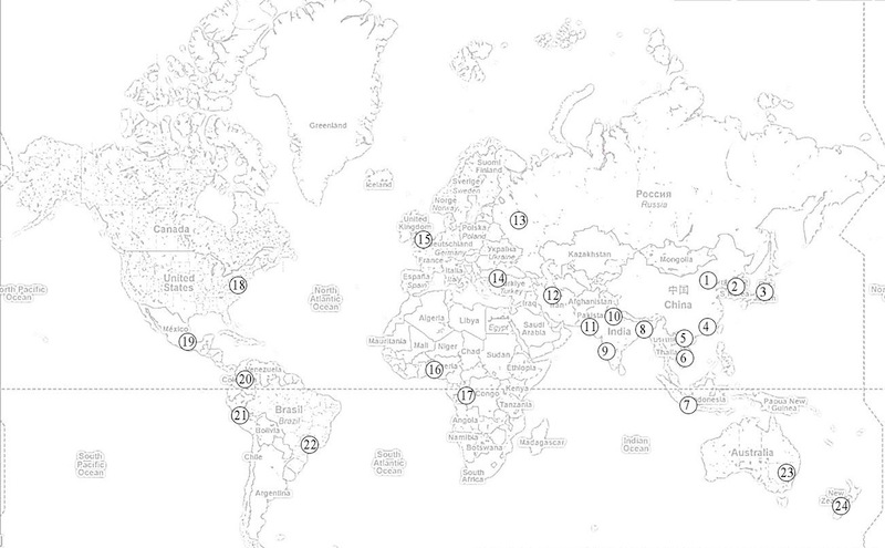
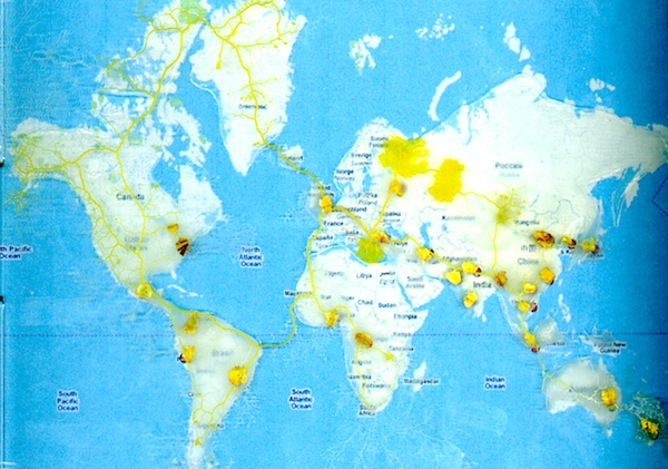
Figure 1: Experimental setup. (a) Configuration of points, representing selected metropolitan or urban areas $\mathbf{U}$. (b) Slime mould P. polycephalum occupies oat flakes representing urban areas $\mathbf{U}$.

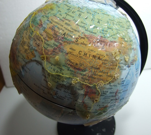
Figure 2: Experimental setup. Globe covered with agar gel is colonised by slime mould P. polycephalum. Oat flakes represent areas of $\mathbf{U}$.

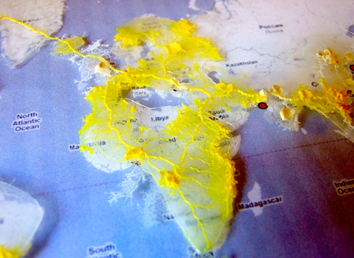
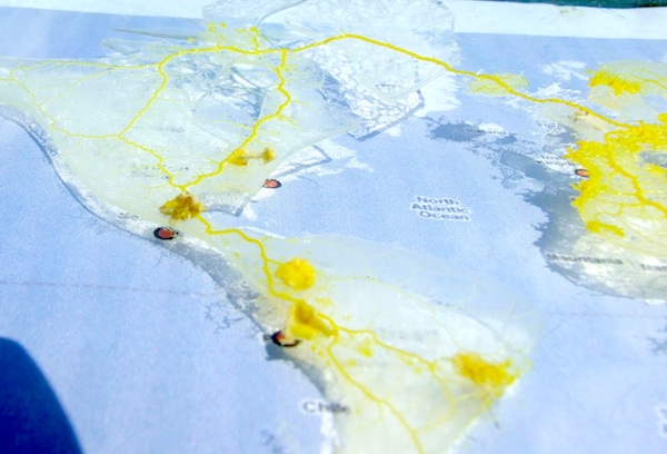
Figure 3: Plasmodium crosses bare space between the continent-shaped agar plates.

We considered 24 metropolitan areas as follows (Fig. 1a):

1. Beijing

2. Seoul

3. Tokyo

4. Hong Kong

5. Ha Noi

6. Ho Chi Minh

7. Jakarta

8. Kolkata

9. Mumbai

10. Delhi

11. Karachi

12. Tehran

13. Moscow

14. Istanbul

15. London

16. Lagos

17. Kinshasa

18. New York

19. Mexico City

20. Bogota

21. Lima

22. Sao Paulo

23. Canberra

24. Wellington

The elements of $\mathbf{U}$ were selected based on their population size, proximity to other urban/metropolitan areas, representativeness of a continent/country. The following area were not chosen for experiments, despite being amongst largest metropolitan areas: Manila is not included due to its proximity to Jakarata; Shanghai due to its proximity to Beijing; Buenos Aires due to its proximity to San Paolo; Osaka-Kobe-Kyoto due their proximity to Tokyo; Dhaka due to its proximity to Kalkutta. The capital cities Canberra and Wellington are by no means in the list of largest cities or metropolitan areas, however they were included to give slime mould a change to move to these countries. To represent areas of $\mathbf{U}$ we placed oat flakes (each flake weights 9–13 mg and is 5–7 mm in diameter) in the positions of agar plate corresponding to the areas (Figs. 1b and 2).

At the beginning of each experiment an oat flake colonised by plasmodium (25–30 mg plasmodial weight) is placed in Beijing area. We have chosen Beijing as a starting point for the slime mould because Beijing is one of the most populated cities in the world [14] and also because the Chinese civilisation is amongst earliest civilisations [26, 26].

We undertook 38 experiments in total: eight experiments with the globe and 30 experiments with the Petri dish. The Petri dishes and the globe with plasmodium were kept in darkness (the globe was placed in a glass container to prevent drying of agar gel), at temperature 22-25${}^{\text{o}}$C, except for observation and image recording. Periodically, the dishes were scanned with an Epson Perfection 4490 scanner and the globe was photographed with FujiFilm FinePix. As exemplified in Fig. 3 absence of a humid growing substrate prevented plasmodium from spreading ’uncontrollably’ into parts of substrate corresponding to oceans and seas yet allowed the plasmodium to migrate between the continents when necessary.

To generalise our experimental results we constructed a Physarum graph with weighted-edges. A Physarum graph is a tuple ${\mathbf{P}}=\langle{\mathbf{U}},{\mathbf{E}},w\rangle$, where $\mathbf{U}$ is a set of urban areas, $\mathbf{E}$ is a set edges, and $w:{\mathbf{E}}\rightarrow[0,1]$ associates each edge of $\mathbf{E}$ with a probability (or weights). For every two regions $a$ and $b$ from $\mathbf{U}$ there is an edge connecting $a$ and $b$ if a plasmodium’s protoplasmic link is recorded at least in one of $k$ experiments, and the edge $(a,b)$ has a probability calculated as a ratio of experiments where protoplasmic link $(a,b)$ occurred in the total number of experiments $k$. We do not take into account the exact configuration of the protoplasmic tubes but merely their existence. Further we will be dealing with threshold Physarum graphs $\mathbf{P}(\theta)=\langle{\mathbf{U}},T({\mathbf{E}}),w,\theta\rangle$. The threshold Physarum graph is obtained from Physarum graph by the transformation: $T({\mathbf{E}})=\{e\in{\mathbf{E}}:w(e)\geq\theta\}$. That is all edges with weights less than $\theta$ are removed.

3 Results

3.1 Scenarios of colonisation

(a) 1 day

(b) 2 days

(c) 3 days

(d) 4 days

(e) 5 days

Figure 4: Example of plasmodium development on a configuration continent-shaped agar plates.

Scenarios of the plasmodium development in Petri dishes and on the globe are strikingly similar. Here we consider one example of colonisation of $\mathbf{U}$ in the Petri dish and three examples of the colonisation on the globe. In first day after inoculation in the Petri dish, the plasmodium propagates from Beijing to Seoul and Tokyo in the east; from Beijing to Hong Kong, Ha Noi and Ho Chi Minh in the south; and from Beijing to Kolkata, Mumbai, Delhi and Karachi in the west (Fig. 4a). On second day the plasmodium explores the space north of Beijing, links Karachi and Tehran, and Tehran and Istanbul with protoplasmic tubes. It also growth from Istanbul to Moscow and from Moscow to London, and from Tehran to Lagos and Kinshasa (Fig. 4b). The plasmodium grows from London to Iceland, then to Greenland. It propagates from Greenland to Canada and eventually reaches New York and Mexico City on the fifth day of the experiment (Fig. 4c). The final stage of spanning $\mathbf{U}$ takes place on the sixth day of the experiment: the plasmodium propagates from Mexico City to Bogota and from Bogota to Lima and Sao Paulo. At the same time the plasmodium grows from Ho Chi Minh to Jakarta and from Jakarta to Canberra and Wellington (Fig. 4d). As soon as all sources of nutrients, representing the areas of $\mathbf{U}$, are spanned by the plasmodium, the plasmodium remains in its configuration for a couple of days (Fig. 4c). By that time the nutrients become depleted, and the substrate contaminated with products of metabolism and the plasmodium tries to migrate to other areas and/or form sclerotium.

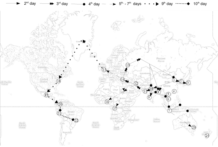
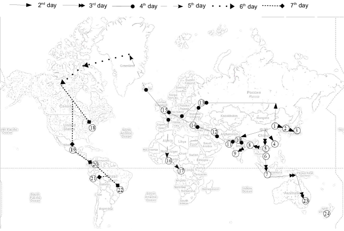
Figure 5: Two scenarios of plasmodial active zones propagation on the globe.

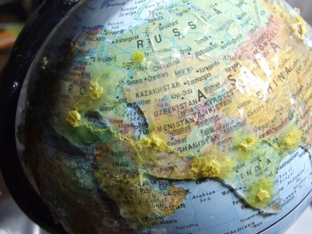
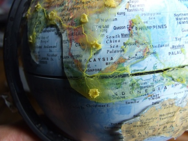
Figure 6: Experimental examples of scenario Fig. 5a. (a) Propagation of slime mould from Karachi to Tehran to Istanbul to Moscow on the third day after inoculation. (b) On the fourth day of experiment plasmodium links Ha Noi to Ho Chi Minh to Jakarta with its protoplasmic tubes and explores space east of Jakarta. (c) Plasmodium’s active zone enters Australia at the port Derby.

Two examples shown in Fig. 5. demonstrate that colonisation of East and South Asia can go by different scenarios however propagations towards Western Europe and Americas have matching trajectories. Let us consider scenario in Fig. 5a. In the second day after inoculation plasmodium propagates from Beijing to Seoul and then to Tokyo, and from Beijing to Delhi and to Kolkata, and from Delhi to Karachi and to Mumbai. On the third day, plasmodium propagates from Karachi to Tehran to Istanbul to Moscow (Fig. 6). It then continuous to explore space north-east of Moscow. On the fourth day plasmodium develops protoplasmic links from Delhi to Kolkata, from Kolkata to Ha Noi and Ho Chi Minh, and from Ho Chi Minh to Jakarta; and, completes the route from Moscow to Beijing. It also explores space east of Jakarta (Fig. 6). On the fifth, sixth and seventh days slime mould propagates from Jakarta to Canberra (Fig. 6), and from Istanbul to London. The plasmodium reaches New York from London via Iceland, Greenland and Canada on ninth day after inoculation in Beijing. Then it propagates from New York to Mexico City, Bogota, Lima and Sao Paulo (Fig. 5a).

Early stages of colonisation (Fig. 5a) show the following priorities of the plasmodium’s development: east then west then south. The scenario with early development: east then south then west, is shown in Fig. 5b and illustrated in Figs. 7, 7, 7, 7.

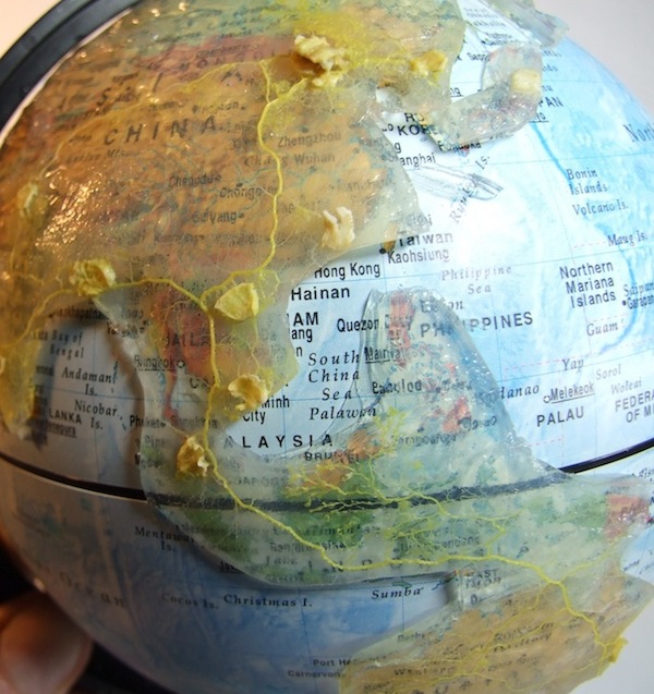
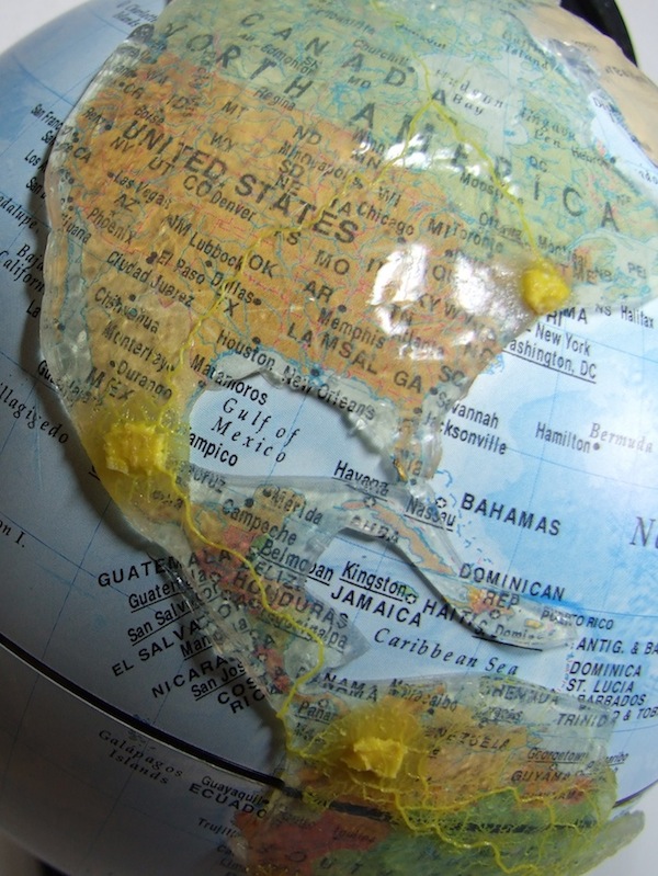
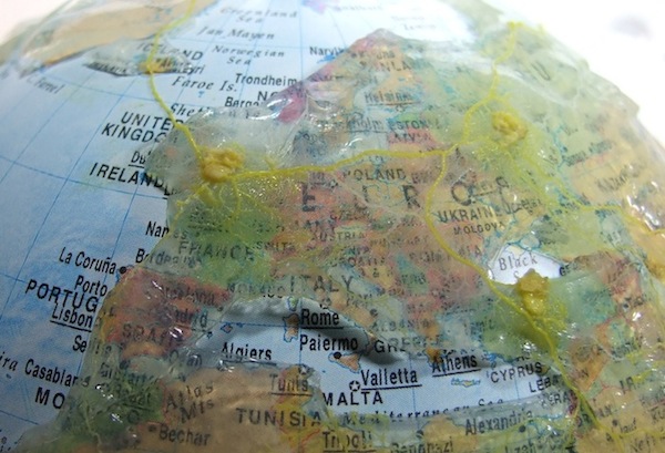
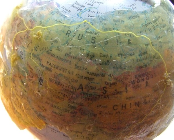
Figure 7: Illustrations of the scenario Fig. 5b. 7 Plasmodium propagates from South-East Asia to Australia. 7 Plasmodium propagates west and north-west. 7 Plasmodium reaches USA via Iceland, Greenland and Canada and then spans Latin America. 7 Transport link between Beijing and London.

In first two days after inoculation in Beijing the plasmodium propagates to Seoul and Tokyo in the east, to Delhi in the south-west and Hong Kong in the south-east. It also ventures north to Siberia. On the third day the plasmodium grows from Ha Noi to Kolkata and Ho Chi Minh, from Ho Chi Minh to Jakarta and Canberra (Fig. 7). On the forth day the plasmodium propagates from Delhi to Karachi, Tehran, Istanbul, Moscow, London, and ventures from London to Iceland (Fig. 7). Protoplasmic links between London and Lagos and Kinshasa are developed by the slime mould at the fifth day of the experiment. On the sixth and seventh days plasmodium crosses Greenland and Canada towards USA. It firstly reaches New York and then propagates towards Mexico City, from where it spans Bogota, Lima and Sao Paulo (Fig. 7). This scenarios also displays a pronounced transport link between Beijing and London (Fig. 7).

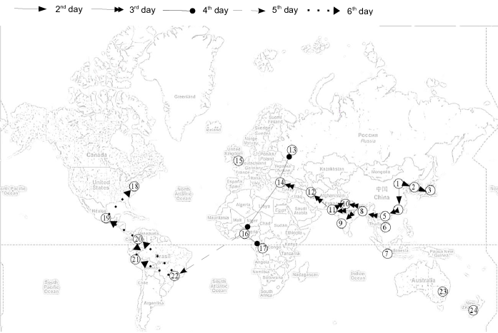
Figure 8: Examples of incomplete spanning of urban areas. Trajectories of plasmodial active zone propagation in ten days of experiment.

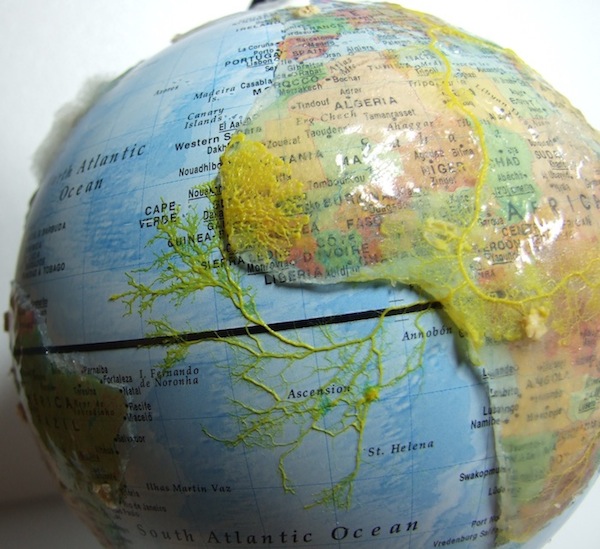
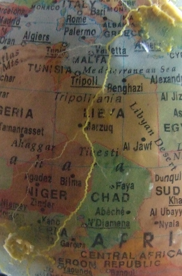
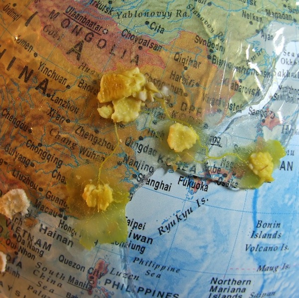
Figure 9: Illustration of the scenario Fig. 8. 9 Plasmodium crosses South Atlantic from West Africa to South America. 9 Protoplasmic tube connecting Istanbul to Lagos develops on the fourth day of experiment. 9 Transport links Beijing, Seoul and Tokyo, and Beijing and Hong Kong are established in two days after inoculation. 9 Chain Hong Kong– Ha Noi– Kolkata– Delhi– Karachi– Tehran– Istanbul is developed on the third day of experiment.

Example of incomplete spanning is shown in Fig. 8. Transport links between Beijing, Seoul and Tokyo, and Beijing and Hong Kong are established in two days after inoculation (Fig. 9). On the third day the plasmodium connects the following areas by the chain of protoplasmic tubes Hong Kong– Ha Noi– Kolkata– Delhi– Karachi– Tehran– Istanbul (Fig. 9). Moscow and Lagos and Kinshasa are spanned by the protoplasmic network on the fourth day of colonisation (Fig. 9). It takes slime mould one more day to cross South Atlantic to make the link between Lagos and Sao Paulo (Fig. 9). Protoplasmic links (Sao Paulo, Lima), (Sao Paulo, Bogota), (Bogota, Mexico City), (Mexico City, New York) are grown on the sixth day of the experiment (Fig. 8.).

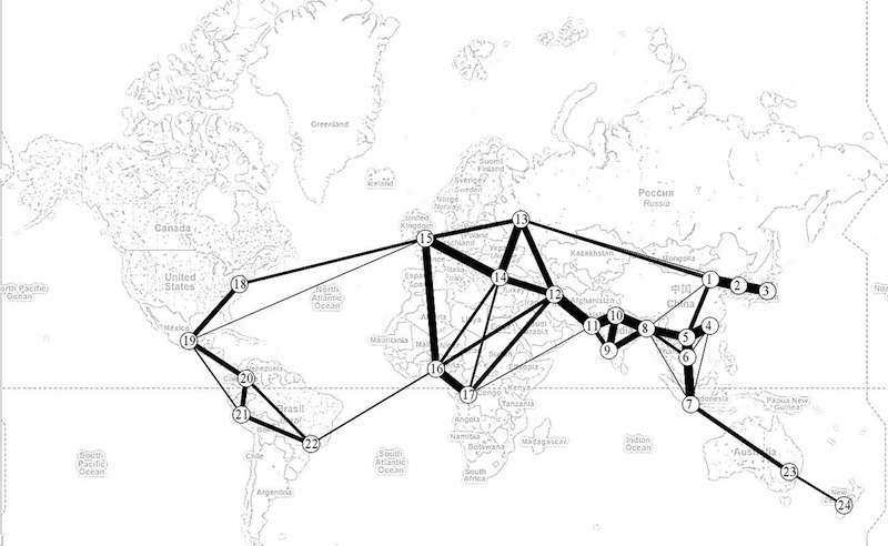
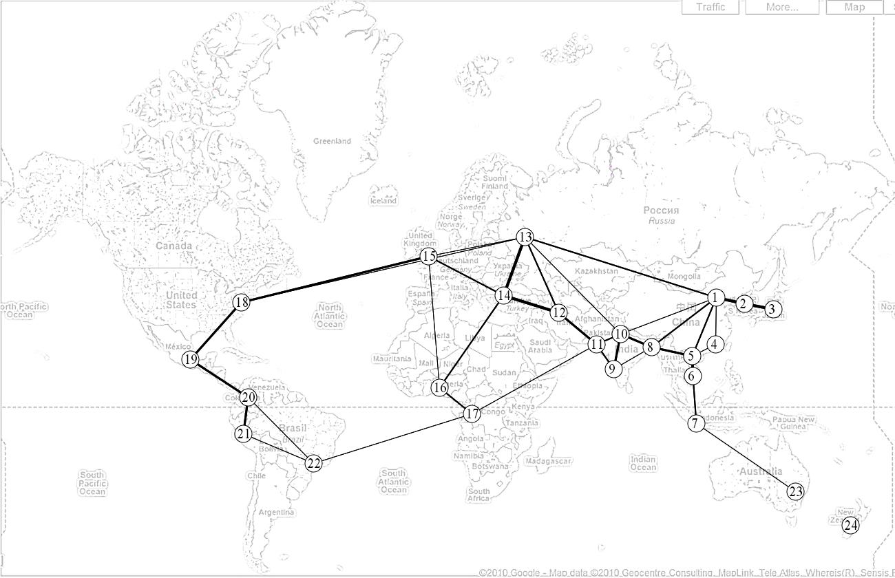
Figure 10: Physarum graphs obtained from experiments in (a) the Petri dishes, P-graph, and (b) the globe, G-graph. Thickness of a line is proportional to the line’s weight.

Generalised Physarum graphs derived from experiments in Petri dishes (let us call them P-graphs) and the globe (G-graphs) are shown in Fig. 10. P-graphs represent G-graphs sufficiently. Only three edges (albeit represented in one experiment each) of P-graphs are not represented by G-graphs: (Kinshasa, Sao Paulo), (Moscow, Istanbul) and (Beijing, Hong Kong). In contrast, eight edges of P-graphs are not represented by G-graphs: (Hong Kong, Jakarta), (Ha Noi, Ho Chi Minh), (Jakarta, Kolkata), (Tehran, Lagos), (Istanbul, Kinshasa), (London, Mexico City), (Mexico City, Bogota) and (Lagos, Sao Paulo). Further in the paper we consider generalised Physarum graphs as a union of P- and G-graphs.

(a) $\theta=\frac{1}{38}$

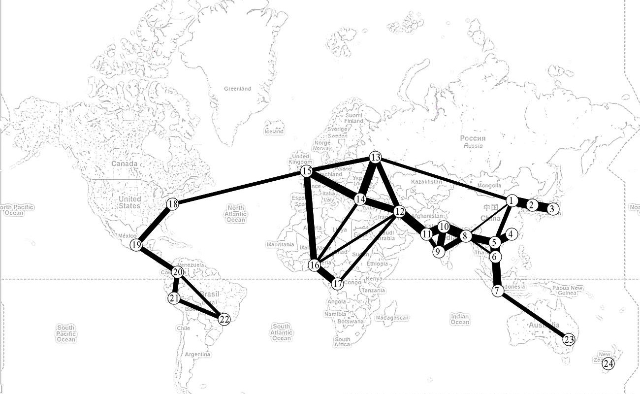
(b) $\theta=\frac{6}{38}$

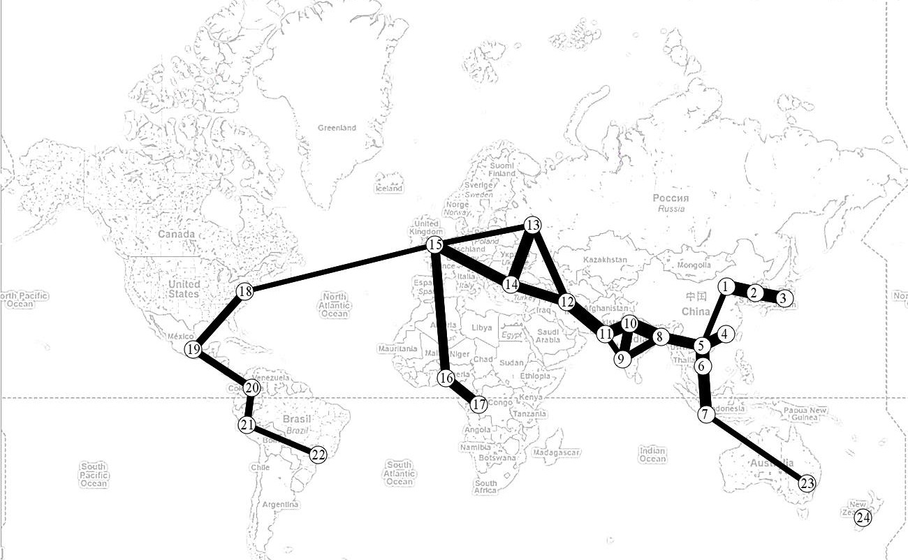
(c) $\theta=\frac{14}{38}$

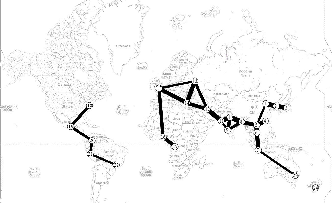
(d) $\theta=\frac{15}{38}$

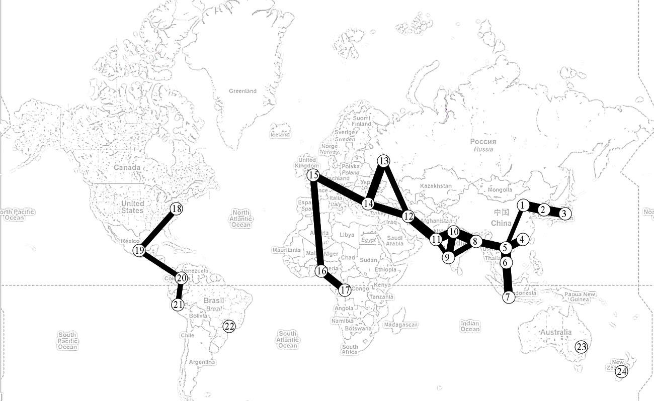
(e) $\theta=\frac{16}{38}$

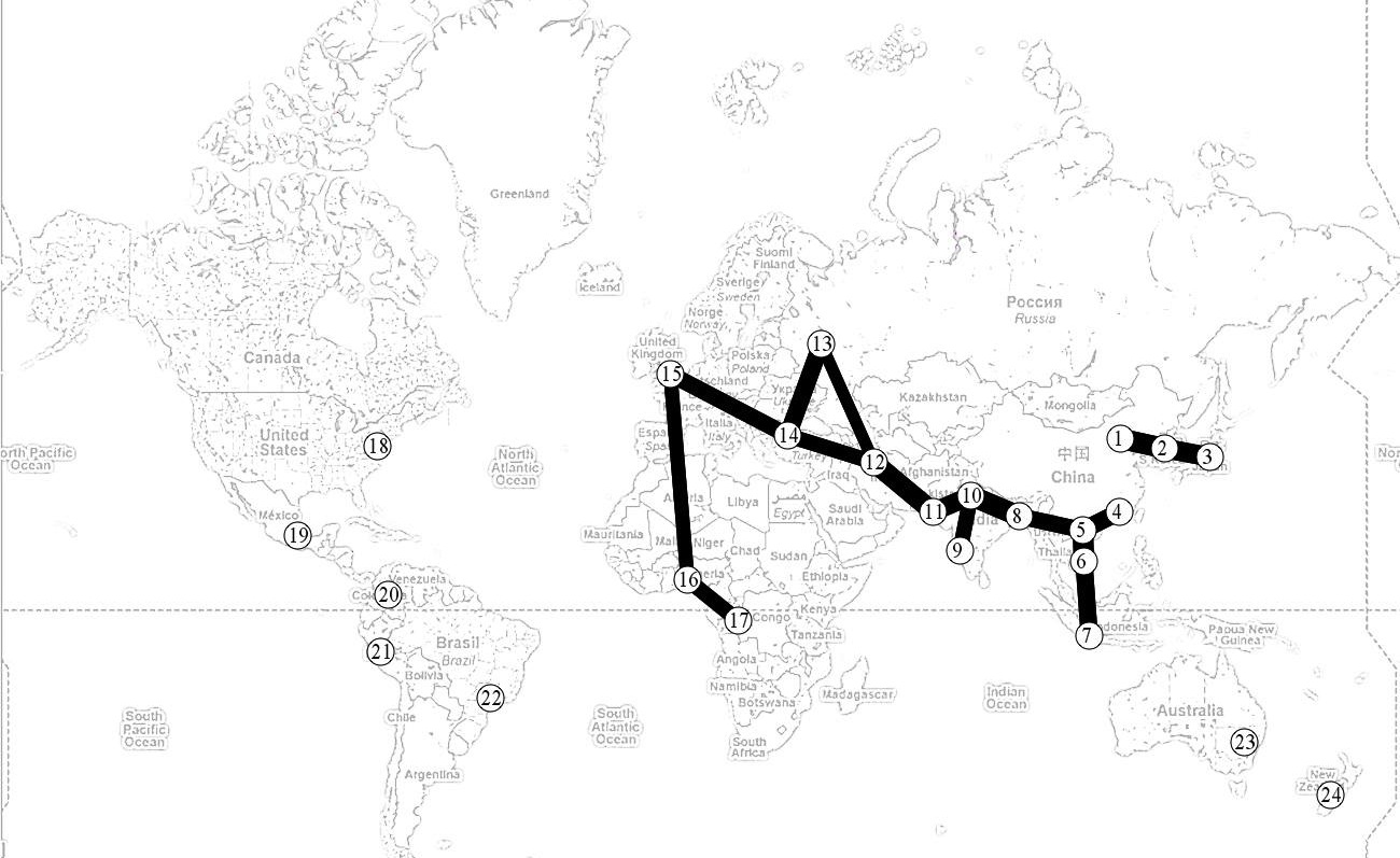
(f) $\theta=\frac{22}{38}$

(g) $\theta=\frac{23}{38}$

Figure 11: Generalized Physarum graphs $\mathbf{P}(\theta)$ for selected values of $\theta$.

Generalised Physarum graphs for critical values of $\theta$ are shown in Fig. 10. Generalised Physarum graphs $\mathbf{P}(\theta)$ are sub-graphs of P- and G-graphs for $\theta\geq\frac{14}{38}$. Physarum graphs are planar for $\theta\geq\frac{6}{38}$ however with acquiring planarity the Physarum graph $\mathbf{P}(\frac{6}{38})$ loses connectivity and Wellington becomes isolated (Fig. 10b). The highest value of $\theta$ for which graph $\mathbf{P}(\theta)-\{$Wellington $\}$ remains connected is $\frac{14}{38}$ (Fig. 10c). When $\theta$ increases to $\frac{15}{38}$ Americas become disconnected from Eurasia and Africa, and American transport pathways become a single chain New York– Mexico City– Bogota– Lima– Sao Paulo (Fig. 10d). Further increase of $\theta$ to $\frac{16}{38}$ leads to isolation of Sao Paulo and Canberra (Fig. 10e).

For $\theta=\frac{22}{38}$ all Americas areas of $\mathbf{U}$ become isolated and the transport network at this continent virtually disappears. The graph $\mathbf{P}(\frac{22}{38})$ has two components of connectivity:

• the chain Beijing– Seoul– Tokyo

• the component consisting of the chain Jakarta– Ho Chi Minh– Kolkata– Delhi– Tehran– Istanbul– London– Lagos– Kinshasa with two branches Ha Noi– Hong Kong and Delhi– Mumbai attached and the cycle Tehran– Moscow– Istanbul– Tehran (Fig. 10f).

Generalised Physarum graph is transformed to the acyclic graph at $\theta=\frac{23}{38}$ when the edge (Tehran, Moscow) becomes cut off (Fig. 10g.)

3.2 Proximity graphs

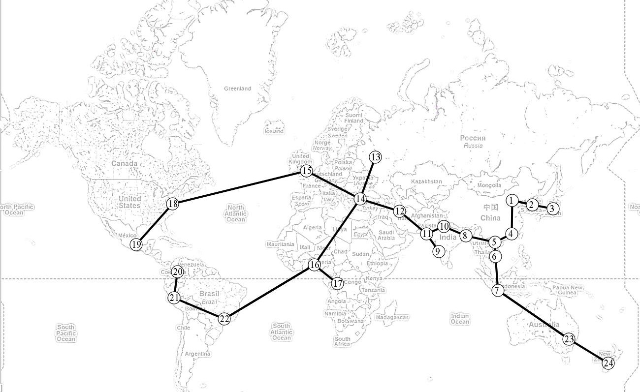
(a) $\mathbf{MST}$

(b) $\mathbf{RNG}$

(c) $\mathbf{GG}$

Figure 12: Relative neighbourhood graph (a) and Gabriel graph (b) constructed on urban areas of $\mathbf{U}$.

(a) $\mathbf{MST}\cap\mathbf{P}(\frac{1}{38})$

(b) $\mathbf{RNG}\cap\mathbf{P}(\frac{1}{38})$

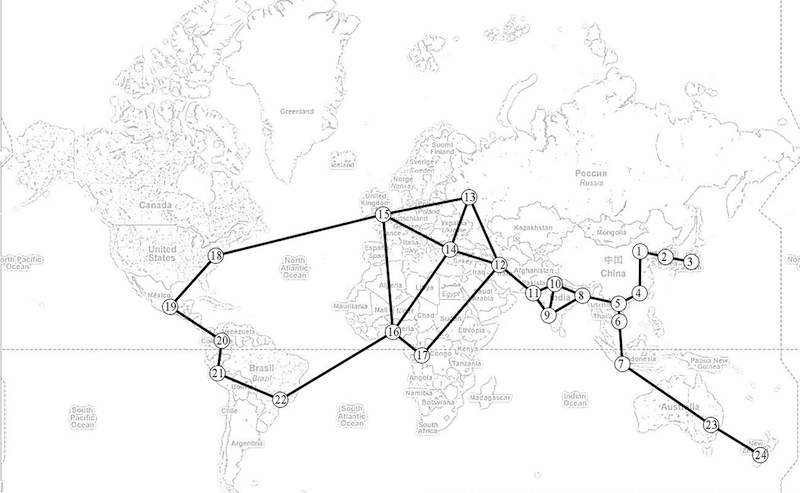
(c) $\mathbf{GG}\cap\mathbf{P}(\frac{1}{38})$

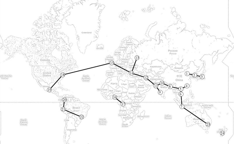
(d) $\mathbf{MST}\cap\mathbf{P}(\frac{14}{38})$

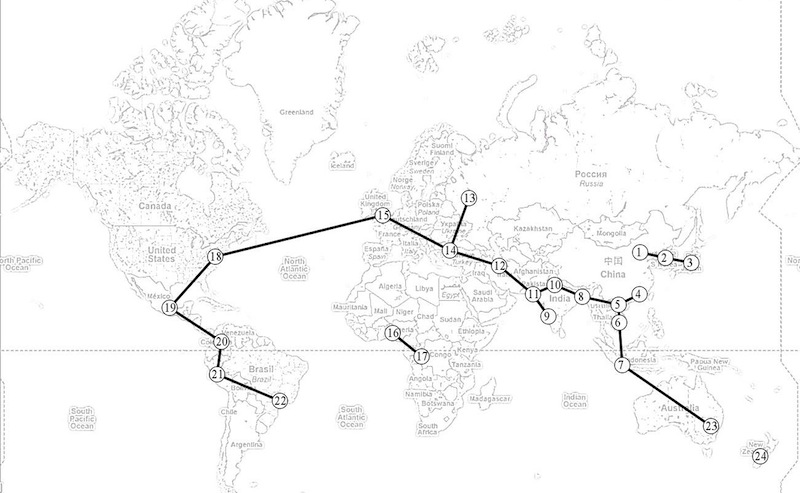
(e) $\mathbf{RNG}\cap\mathbf{P}(\frac{14}{38})$

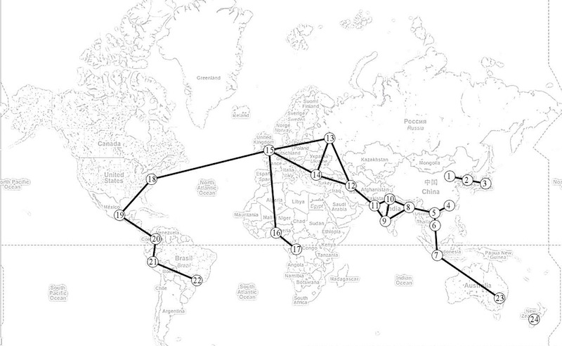
(f) $\mathbf{GG}\cap\mathbf{P}(\frac{14}{38})$

Figure 13: Intersections of generalised Physarum graphs (abc) $\mathbf{P}(\frac{1}{38})$ and (def) $\mathbf{P}(\frac{14}{38})$ with proximity graphs: (ad) minimum spanning tree $\mathbf{MST}$, (be) relative neighbourhood graph $\mathbf{RNG}$, (cf) Gabriel graph $\mathbf{GG}$.

A planar graph consists of nodes which are points of the Euclidean plane and edges which are straight segments connecting the points. A planar proximity graph is a planar graph where two points are connected by an edge if they are close in some sense. A pair of points is assigned a certain neighbourhood, and points of the pair are connected by an edge if their neighbourhood is empty. Here we consider the most common proximity graphs as follows.

$\mathbf{MST}$: The Euclidean minimum spanning tree [32] is a connected acyclic graph which has minimum possible sum of edges’ lengths (Fig. 12a).

$\mathbf{RNG}$: Points $a$ and $b$ are connected by an edge in the Relative Neighbourhood Graph if no other point $c$ is closer to $a$ and $b$ than $dist(a,b)$ [43] (Fig. 12b).

$\mathbf{GG}$: Points $a$ and $b$ are connected by an edge in the Gabriel Graph if disc with diameter $dist(a,b)$ centred in middle of the segment $ab$ is empty [16, 25] (Fig. 12a).

In general, the graphs relate as $\mathbf{MST}\subseteq\mathbf{RNG}\subseteq\mathbf{GG}$ [43, 25, 21]; this is called Toussaint hierarchy.

Why do we need to compare Physarum graphs with the proximity graphs $\mathbf{MST}$, $\mathbf{RNG}$ and $\mathbf{GG}$? The minimum spanning tree helps to evaluate optimality of the protoplasmic networks: minimal distances of nutrient transportation yet complete covering of the sources of nutrients (sites of $\mathbf{U}$). Being an acyclic graph the spanning tree is sensitive to a structural damage. Removal of a single edge might transform the spanning tree to two disconnected trees. The relative neighbourhood graph and the Gabriel graph show higher degree of fault-tolerance (depending on exact configuration of nodes). It also considered to be optimal in terms of total edge length and travel distance. The graphs $\mathbf{RNG}$ and $\mathbf{GG}$ are used in geographical variational analysis [16, 25], simulation of epidemics [42], and design of ad hoc wireless networks [23, 37, 33, 27, 45]. The proximity graphs, especially $\mathbf{RNG}$, are invaluable in simulation of human-made, road networks; these graphs are validated in studies of Tsukuba central district road networks [46, 47]. Gabriel graphs, particularly their relaxed versions [13] are an ideal tool for path finding and online routing on planar graphs [12].

Intersections of generalised Physarum graphs with the proximity graphs is shown in (Fig. 13).

Finding 1.

The minimum spanning tree and the relative neighbourhood graph are sub-graphs of $\mathbf{P}(\frac{1}{38})$. Gabriel graph would be a sub-graph of $\mathbf{P}(\frac{1}{38})$ if the Physarum graph had the edges (Hong Kong, Seoul) and (New York, Bogota).

The $\mathbf{MST}$ differs from $\mathbf{RNG}$ only by absence of the single edge (Mexico City, Bogota), the rest is the same and is matched by edges of the generalised Physarum graph $\mathbf{P}(\frac{1}{38})$ (Fig. 13ab). The fact that $\mathbf{GG}\subseteq\mathbf{P}(\frac{14}{38})\cup$(Hong Kong, Seoul)$\cup$(Mexico City, Bogota) (Fig. 13c) plays against the geographical validity of the Gabriel graph. The only physically possible routes from New York to Bogota and from Hong Kong to Seoul are maritime routes; overland route from New York to Bogota is passing via Mexico City and from Hong Kong to Seoul via Beijing.

Finding 2.

The longest chain in $\mathbf{MST}\cap\mathbf{P}(\frac{14}{38})$ is $C_{1}$=(Canberra– Jakarta– Ho Chi Minh– Ha Noi– Kolkata– Delhi– Karachi– Tehran– Istanbul– London– New York– Mexico City)

Two fragments of the chain $C_{1}$: Jakarta– Ho Chi Minh– Ha Noi and Kolkata to London (Fig. 13d) match the Silk Road, see Sect. 3.3. The chain $C_{1}$ is elongated by segment (Bogota– Lima– Sao Paulo) in $\mathbf{RNG}\cap\mathbf{P}(\frac{14}{38})$ (Fig. 13e) and $\mathbf{GG}\cap\mathbf{P}(\frac{14}{38})$ (Fig. 13f).

3.3 Protoplasmic Networks, the Silk Road and the Asian Highways

Figure 14: Graphs of the Silk Road and the Asian Highways. (a) the Silk Road graph, comprised of the Silk Road (thick line) and associated trade routes (thin lines); the graph is derived from the scheme of Trans-Asian trade 500 BC – AD 750 [36]. (b) the Asian Highway network graph; the graph is derived from the Asian Highway Network Map [34].

To evaluate how well plasmodial networks match large-scale transportation systems we compare generalised Physarum graphs with graphs derived from the Silk Road and the Asia Highway network.

The Silk Road is a long-distance trade route across Asia developed in the first millennium to transport goods between China and Western Asia and Northern Europe [41]. Commonly the Silk Road is comprised of the main overland route from Luoyang to Seleucia/Clesiphon and associated overland and maritime routes reaching as far Japan in the east and as far as Colchester and Holborough in the west [36, 24].

A graph of the Silk Road is shown in Fig. 14a. When constructing the Silk road graph we tracked geographical positions of modern cities along the historical Silk Road and associated trade routes, with minor assumptions. Thus the Silk Road is represented by edge (Beijing, Tehran). The road actually started at Luoyang and passed via Hecatompylos and ended in Ctesiphon. We assumed Hecatompylos was in proximity of Tehran and Beijing is in proximity of Luoyang. Similarly, we assume that edge Delhi to Kolkata corresponds to the trade route connecting Mathura (proximity of Delhi) and Tampluk via Pataliputra (proximity of Kolkata). Link (Tokyo, Hong Kong) corresponds to a maritime route from south of Japan to Oc Eo via Guangzhou and passing between the continental China and Hong Kong island. The edge (Tehran, Istanbul) represents land route from Hecatompylos to Dura Europos and Antioch combined with maritime trade route from Antioch to Constantinple. The edge (Istanbul, London) represents maritime route Constantinople – Athens – Rome – Massilia – Colchester.

The Asian Highways is a network of roads selected for regional transport cooperation “initiative aimed at enhancing efficiency and development of the road transport infrastructure in Asia” [34]. The Asian Highway network consists of 141,000 km of roads running across 32 member States. When constructing Asian Highway graph (Fig. 14b) we adopted the following match between the graph’s edges and the highways (see map of the Asian Highway network in [34]):

• (Beijing, Seoul): potential route AH1 Beijing to Shenyang and existing route AH1 Shenyang to Seoul;

• (Beijing, Hong Kong): route AH1 Beijing to Hong Kong via Zhengzhou, Xinyang, Xianglan;

• (Beijing, Delhi): route A1 Beijing to Zhengzhou, potential routes AH34 Zhengzhou to Xi’an, AH5 Xi’an to Langzhou, AH42 Langzhou to Lhasa, and final existing routes AH42 Lhasa to Zhangmu and AH2 Zhangmu to Delhi;

• (Beijing, Tehran): comprised of segments of the following highways (ordered from Beijing to Tehran) AH1, AH34, AH5, AH4, AH65, AH62, AH76, AH1;

• (Beijing, Moscow): AH3 Beijing to Ulan Ude, AH5 from Ulan Ude to Moscow via Irkutsk, Novosibirsk, Omsk, Petropavlosk, Chelyabinsk, Samar;

• (Seoul, Tokyo): maritime route Pusan to Fukuoka and overland route AH1 Fukuoka to Tokyo;

• (Hong Kong, Ha Noi): potential route AH1 Guangzhou to Nanning, AH1 Nanning to Hanoi;

• (Ha Noi, Ho Chi Minh): AH1;

• (Ha Noi, Kolkata): AH14 Hanoi – Kummig – Mandalay and AH1 Mandalay – Dispur – Kolkata;

• (Ho Chi Minh, Jakarta): AH1 Ho Chi Minh to Kabin Bun, AH19 Kabin Bun to Bangkok, AH2 Bangkok to Hat Yai, AH18 Hat Yai to Singapore, and maritime Singapore to Jakarta;

• (Kolkata, Mumbai): AH46 and AH47;

• (Kolkata, Delhi): AH1;

• (Delhi, Karachi): AH1 Delhi to Lahore, AH2 Lahore to Rohn, AH4 Rohn to Karachi;

• (Karachi, Tehran): AH7 Karachi to Kandahar and AH1 Kandahar – Dilaram – Herat – Zhabzevar – Tehran;

• (Tehran, Moscow): AH8 Tehran – Baku – Astahan – Volgograd – Moscow;

• (Tehran, Istanbul): AH1 Tehran – Yerevan – Ankara and AH5 Ankara to Istanbul.

The Asian Highway graph has the same number of edges as the Silk Road graph however they are not isomorphic (Fig. 14).

Finding 3.

Slime mould P. polycephalum approximates over 76% of the Silk Road routes and the Asian Highway routes.

Physarum graph $\mathbf{P}(\frac{6}{38})$ (Fig. 11b) approximates 13 of 17 edges of the Silk Road graph(Fig. 14a) and also 13 of 17 edges of the Asian Highway graph (Fig. 14b). Physarum graph $\mathbf{P}(\frac{14}{38})$ (Fig. 11c) approximates 11 of 17 edges of the Silk Road graph and also 11 of 17 edges of the Asian Highway graph.

Finding 4.

Transport links (Beijing, Tehran) and (Beijing, Hong Kong) of the Silk Road and the Asian Highway network are never approximated by P. polycephalum.

The following routes of the Silk Road are never approximated by any Physarum graph: (Delhi, Tehran), (Beijing, Hong Kong), (Tokyo, Hong Kong), (Hong Kong, Jakarta). Routes (Beijing, Tehran) and (Beijing, Kolkata) are approximated by $\mathbf{P}(\frac{6}{38})$ but not $\mathbf{P}(\frac{14}{38})$.

The following routes of the Asian highways are not approximated by any Physarum graph: (Beijing, Tehran), (Beijing, Hong Kong), (Beijing, Delhi) and (Jakarta, Kolkata). Routes (Beijing, Moscow) and (Ho Chi Minh, Kolkata) are approximated by $\mathbf{P}(\frac{6}{38})$ but not $\mathbf{P}(\frac{14}{38})$.

4 Conclusions

To imitate a hypothetical scenario of the World’s colonisation and emergence of principal transport networks we represented the continents with geometrically-shaped plates of non-nutrient agar and the major metropolitan areas with sources of nutrients and inoculated plasmodium of P. polycephalum in Beijing. We analysed scenarios of the plasmodium propagation and colonisation of the metropolitan areas. We derived weighted generalised Physarum graphs from the protoplasmic networks recorded in the laboratory experiments.

We found that the Physarum graphs include basic proximity graphs — the minimum spanning tree, the relative neighbourhood graph and the Gabriel graph constructed on the metropolitan areas — as their sub-graphs. The longest chain of transport links presented in the minimum spanning tree and in the Physarum graph with edge weights exceeding 0.36 is Canberra– Jakarta– Ho Chi Minh– Ha Noi– Kolkata– Delhi– Karachi– Tehran– Istanbul– London– New York– Mexico City. We found that slime mould P. polycephalum approximates over 76% of the Silk Road routes and the Asian Highway network. Transport links (Beijing, Tehran) and (Beijing, Hong Kong) of the Silk Road and the Asian Highway network are never approximated by P. polycephalum.

We believe our experimental results will inspire further thoughts, paradigms and approaches for re-evaluation of historical findings on the emergence of ancient roads and will help to design future trans-continental pathways. The results could be also applied in analysis of pandemics’ dynamics [11, 18] and in shaping unorthodox approaches to prediction of international military conflicts and battlefield operations [19].

References

- [1] Adamatzky A., De Lacy Costello B., Asai T. Reaction-Diffusion Computers, Elsevier, Amsterdam, 2005.
- [2] Adamatzky A. Developing proximity graphs by Physarum Polycephalum: Does the plasmodium follow Toussaint hierarchy? Parallel Processing Letters 19 (2008) 105–127.
- [3] Adamatzky A. and Jones J. Road planning with slime mould: If Physarum built motorways it would route M6/M74 through Newcastle arXiv:0912.3967v1 [nlin.PS] (Dec 2009). Int J Bifurcaton and Chaos 20 (2010) 3065–3084.
- [4] Adamatzky A., Martinez G. J., Chapa-Vergara S. V., Asomoza-Palacio R., Stephens C. R. Approximating Mexican highways with slime mould. Natural Computing 10 (2010) 1195–1214.
- [5] Adamatzky A. Hot ice computer. Physics Lett A 347 (2009) 264–271.
- [6] Adamatzky A. and Alonso-Sanz R. Rebuilding Iberian motorways with slime mould. Biosystems 105 (2010) 89–100.
- [7] Adamatzky A. Physarum Machines: Making Computers from Slime Mould (World Scientific, 2010).
- [8] Adamatzky A. and de Oliveira P.P.B. Brazilian highways from slime mold’s point of view. Kybernetes 11 (2011).
- [9] Adamatzky A. and Prokopenko M. Slime mould evaluation of Australian motorways, Int J Parallel, Emergent and Distributed Systems (2011) DOI:10.1080/17445760.2011.616204
- [10] Adamatzky A. and Akl S.G. Trans-Canada Slimeways: Slime mould imitates the Canadian transport network (2011) arXiv:1105.5084v1 [nlin.PS]
- [11] Beck E.J. Mays N., Whiteside A.W. (Eds.) The HIV Pandemic: Local and Global Implications. (Oxford University Press, 2008).
- [12] Bose P. and Morin P. Competitive online routing in geometric graphs. Theoretical Computer Science 324 (2004) 273 -288.
- [13] Bose P., Cardinal J., Collette S., Demaine E. D., Polop B., Taslakian P., Zehk N. Relaxed Gabriel Graphs. In: 21st Canadian Conference on Computational Geometry 2009, Vancouver, BC, August 17 19, 2009.
- [14] Beijing Municipal Bureau of Statistics (2011). http://www.bjstats.gov.cn/esite/
- [15] Dorigo M. and Stutzle T. Ant Colony Optimization MIT Press, 2004.
- [16] Gabriel K. R. and R. R. Sokal. A new statistical approach to geographic variation analysis. Systematic Zoology, 18 (1969) 259–278.
- [17] Gernet J. A History of Chinese Civilization. (Cambridge University Press, 1996).
- [18] Haour-Knipe M. and Rector R. (Ed.itor) Crossing Borders: Migration, Ethnicity and AIDS (Social Aspects of AIDS) (Taylor & Francis, 1996.)
- [19] Ilachinski A. Artificial War: Multiagent-Based Simulation of Combat (World Scientific, 2004).
- [20] Jaromczyk J.W. and Kowaluk M. A note on relative neighbourhood graphs Proc. 3rd Ann. Symp. Computational Geometry, 1987, 233–241.
- [21] Jaromczyk J. W. and G. T. Toussaint, Relative neighborhood graphs and their relatives. Proc. IEEE 80 (1992) 1502–1517.
- [22] Jarrett T. C., Ashton D. J., Fricker M., Johnson N. F. Interplay between function and structure in complex networks Phys. Rev. E 74 (2006) , 026116.
- [23] Li X.-Y. Application of computation geometry in wireless networks. In: Cheng X., Huang X., Du D.-Z. (Eds.) Ad Hoc Wireless Networking (Kluwer Academic Publishers, 2004) 197–264.
- [24] Liu X.s The Silk Road in World History (Oxford University Press, 2010).
- [25] Matula D. W. and Sokal R. R. Properties of Gabriel graphs relevant to geographical variation research and the clustering of points in the same plane. Geographical Analysis 12 (1984) 205–222.
- [26] Makeham J. and Buell P. D. China: The World’s Oldest Living Civilization Revealed (Thames & Hudson, 2008).
- [27] Muhammad R. B. A distributed graph algorithm for geometric routing in ad hoc wireless networks. J Networks 2 (2007) 49–57.
- [28] Nakagaki T., Yamada H., and Toth A. Maze-solving by an amoeboid organism. Nature 407 (2000) 470.
- [29] Nakagaki T., Yamada H., and Toth A. Path-finding by tube morphogenesis in an amoeboid organism. Biophys. Chem. 92 (2001) 47- 52.
- [30] Nakagaki T., Iima M., Ueda T., Nishiura Y., Saigusa T., Tero A., Kobayashi R., and Showalter K. Minimum-risk path finding by an adaptive amoeba network. Phys. Rev. Lett. 99 (2007) 068104.
- [31] Nakagaki T., Makoto I., Ueda T., Nishiura T., Saigusa T., Tero A., Kobayashi R., and Showalter K. Minimum-risk path finding by an adaptive amoebal network. Phys. Rev. Lett. 99 (2007) 68104.
- [32] Nesetril J., Milkova E., Nesetrilova H., Otakar Boruvka on minimum spanning tree problem, Discrete Mathematics 233 (2001) 3–36.
- [33] Santi P. Topology Control in Wireless Ad Hoc and Sensor Networks (Wiley, 2005).
- [34] Priority Investment Needs for the Development of the Asian Highway Network. Economic and Social Commission for Asia and the Pacific. (United Nations, New York, 2006), p. 2.
- [35] Reyes D. R., Ghanem M. G., George M. Glow discharge in micro fluidic chips for visible analog computing. Lab on a Chip 1 (2002) 113–116.
- [36] Scarre C. (General Editor). Past Worlds. The Times Atlas of Archaeology. (Times Books, 1996), p. 190–191.
- [37] Song W.-Z., Wang Y., Li X.-Y. Localized algorithms for energy efficient topology in wireless ad hoc networks. In: Proc. MobiHoc 2004 (May 24–26, 2004, Roppongi, Japan).
- [38] Stephenson S. L. and Stempen H. Myxomycetes: A Handbook of Slime Molds. (Timber Press, 2000).
- [39] Supowit K.J. The relative neighbourhood graph, with application to minimum spanning tree J. ACM 30 (1988) 428–448.
- [40] Tero A., Takagi S., Saigusa T., Ito K., Bebber D.P., Fricker M.D., Yumiki K., Kobayashi R., Nakagaki T. Rule for biologically inspired adaptive network design. Science 327 (2010) 439–442.
- [41] Thubron C. Shadow of the Silk Road (Harper Perennial, 2008).
- [42] Toroczkai Z. and Guclu H. Proximity networks and epidemics. Physica A 378 (2007) 68. arXiv:physics/0701255v1
- [43] Toussaint G. T., The relative neighborhood graph of a finite planar set, Pattern Recognition 12 (1980) 261–268.
- [44] Tsuda S., Aono M., Gunji Y.-P. Robust and emergent Physarum logical-computing. Biosystems 73 (2004) 45–55.
- [45] Wan P.-J., Yi C.-W. On the longest edge of Gabriel Graphs in wireless ad hoc networks. IEEE Trans. on Parallel and Distributed Systems 18 (2007) 111–125.
- [46] Watanabe D. A study on analyzing the road network pattern using proximity graphs. J of the City Planning Institute of Japan 40 (2005) 133–138.
- [47] Watanabe D. Evaluating the configuration and the travel efficiency on proximity graphs as transportation networks. Forma 23 (2008) 81-–87.