Graphene hyperlens for terahertz radiation

Abstract

We propose a graphene hyperlens for the terahertz (THz) range. We employ and numerically examine a structured graphene-dielectric multilayered stack that is an analogue of a metallic wire medium. As an example of the graphene hyperlens in action we demonstrate an imaging of two point sources separated with distance $\lambda_{0}/5$. An advantage of such a hyperlens as compared to a metallic one is the tunability of its properties by changing the chemical potential of graphene. We also propose a method to retrieve the hyperbolic dispersion, check the effective medium approximation and retrieve the effective permittivity tensor.

Rapidly developing terahertz (THz) science and technology acquired a great deal of attention in recent years due to an enormous potential for spectroscopy, communication, defense and biomedical imaging Tonouchi (2007); Jepsen et al. (2011); Kleine-Ostmann and Nagatsuma (2011). The natural diffraction limit, however, restricts the resolution of the standard THz imaging systems to about a wavelength, which is relatively large (300 $\mu$m in the free space at 1 THz). To overcome this restriction one can use the scanning near-field THz microscopy that allows for even submicrometer resolution in the scattering (apertureless) configuration Kersting et al. (2005),but such technique is slow. Another solution is to use a metamaterial lens with artificially engineered properties, for example, a negative index lens Pendry (2000) or hyperbolic-dispersion lens (hyperlens) Jacob et al. (2006). While the negative-index material lens is far from being implemented into the imaging systems due to high losses and narrow resonant frequency range, the hyperlens has been experimentally demonstrated in the microwave Belov et al. (2006) and optical Liu et al. (2007) regimes. The hyperlens is able to convert evanescent waves into propagating ones and to magnify a subwavelength image so that it can be captured by a standard imaging system, a microscope, for example.

A hyperlens usually consists of metal-dielectric layers (in ultraviolet and optical ranges) or of metallic wires (infrared and microwave ranges). Due to the employment of metal the properties of the hyperlens cannot be tuned after fabrication. In contrast to metal, graphene, a two-dimentional material with striking electronic, mechanical and optical propertiesSavage (2012), supports surface plasmon polaritons in the THz range Jablan et al. (2009); Ju et al. (2011a) that are widely tunable by the change of graphene’s electrochemical potential via chemical doping, magnetic field or electrostatic gating Chen et al. (2012). Many plasmonic effects and photonic applications of graphene have been proposed Lee et al. ; Liu et al. (2011, 2012); Vakil and Engheta (2011); Tassin et al. (2012); Ju et al. (2011b). Nevertheless, up to our knowledge, no graphene based hyperlens for the THz range has been proposed so far (however, there has been recently reported a graphene and boron nitride hyperlens for the ultraviolet Wang et al. (2012)).

In this letter we propose to use structured graphene for the creation of a hyperlens in the THz range. To support our proposal we investigate the effective properties of the hyperbolic graphene wire medium and then construct a hyperlens out of it. We check numerically the performance of a full-size three-dimensional (3D) and its homogenized two-dimensional (2D) analogue and demonstrate that it has the desired subwavelength resolution and magnification.

Several requirements have to be satisfied for constructing the hyperlens Jacob et al. (2007); Silveirinha et al. (2007). First of all, an indefinite material (the permittivity tensor components have opposite signs) with strong cylindrical anisotropy should be used. Namely the radial permittivity $\varepsilon_{r}$ should be negative ($\varepsilon_{r}<0$) while azimuthal permittivity $\varepsilon_{\theta}$ should be positive ($\varepsilon_{\theta}>0$). In this case the in-plane isofrequency contour is hyperbolic:

$$\frac{q^{2}}{\varepsilon_{\theta}}+\frac{\kappa^{2}}{\varepsilon_{r}}=1,$$ (1)

where $q=k_{r}/k_{0}$ is the normalized radial wavevector component, $\kappa=k_{\theta}/k_{0}$ is the normalized azimuthal wavevector and $k_{0}=2\pi/\lambda_{0}=\omega/c$ is the wavenumber in vacuum. Then the waves with $\kappa>1$, that are evanescent in vacuum, can propagate in the hyperbolic medium. Mathematically this means that for every $\kappa$ there exists a real-valued $q$. Moreover, the dependence $q(\kappa)$ should be as flat as possible. That ensures the same phase velocities for all spatial components (various $\kappa$). There are two possibilities for satisfying this requirement: to select a material with either a large negative $\varepsilon_{r}$ or a small positive $\varepsilon_{\theta}$.

For high transmission propagation losses characterized by ($Im(q)$) should be as small as possible. For the waves with $\kappa\ll 1$ the radial wavevector reduces to $q\thickapprox\sqrt{\varepsilon_{\theta}}$, so it is primarily $\varepsilon_{\theta}$ that determines losses. The incoupling and outcoupling of the waves to the ambient medium should also be efficient. For normally incident waves from a dielectric with a refractive index $n$ onto the flat interface with a hyperbolic medium, the reflection coefficient is $R=\frac{n-q}{n+q}=\frac{n-\sqrt{\varepsilon_{\theta}}}{n+\sqrt{\varepsilon_{\theta}}}$, so in order to minimize reflection one has to match the azimuthal permittivity $\varepsilon_{\theta}$ with the permittivity $\varepsilon=n^{2}$ of the surrounding medium. This requirement limits the range of $\varepsilon_{\theta}$. In addition to that to maximize the hyperlens transmission the Fabry-Perot resonance condition should be satisfied

$$R_{2}-R_{1}=\frac{m\lambda_{\rm{eff}}}{2}=\frac{\pi m}{qk_{0}},$$ (2)

where $R_{1}$ and $R_{2}$ are the inner and outer hyperlens radius, respectively, $\lambda_{\rm{eff}}$ is the effective wavelength and $m$ is an integer number. The ratio of the radii $M=R_{2}/R_{1}$ determines the hyperlens magnification.

Finally, since no natural electromagnetic materials with a strong cylindrical anisotropy exist, artificial effectively homogenous metamaterials have to be used. That means that its lateral geometrical period $P$ should be much (at least 5-10 times) smaller than the period of the wave with the highest $\kappa=\kappa_{max}$. So, for example, if we wish to construct the hyperlens for the free-space wavelength $\lambda_{0}=50\mu$m that supports the wave with the highest $\kappa_{max}=5$, then the lateral period of the metamaterial should not be larger than $P_{\rm{max}}=\frac{1}{10}\frac{\lambda_{0}}{\kappa_{\rm{max}}}=1\mu$m.

First we analyzed the properties of the graphene wire medium itself. Its unit cell is a rectangular block of dielectric ($\varepsilon_{D}=2.34$ corresponding to the low-loss polymer TOPAS) of the size $a_{x}\times a_{y}\times a_{z}=0.2\times 0.05\times 1\mu$m³ ($a_{x},a_{y}\ll P_{\rm{max}}$) with an embedded graphene stripe of the width $w$ depicted in Fig.1a. We described graphene for the simulations in CST CST as a layer of thickness $\Delta=1$ nm with the permittivity $\varepsilon_{G}=\varepsilon_{D}+i\frac{\sigma_{S}}{\varepsilon_{0}\omega\Delta},$ where $\sigma_{S}$ is the surface conductivity of graphene.

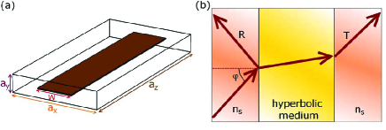
Figure 1: (a) The unit cell of the graphene wire medium consists of a graphene stripe of the width $w$ embedded into a dielectric. (b) To characterize the hyperbolic medium we calculated complex reflection $R$ and transmission $T$ coefficients for various angles of incidence $\varphi$. A block of the hyperbolic medium is placed between high-index $n_{s}$ dielectric layers.

In order to retrieve the dispersion relation $q(\kappa)$ we simulated complex reflection $R$ and transmission $T$ coefficients for various angles of incidence $\varphi$ on a hyperbolic medium slab (see Fig. 1b) with the periodic (unit cell) boundary conditions. We considered TM polarized waves (magnetic field along the $y$-axis). The surrounding medium was a high refractive index $n_{S}$ dielectric. Then for each $\kappa$ and frequency $\omega$ we can restore $q$ Menzel et al. (2008)

$$q=\pm\frac{1}{k_{0}a_{z}}\arccos\frac{1-R^{2}+T^{2}}{2T}+\frac{2\pi m}{k_{0}a_{z}},$$ (3)

where $m$ is an integer number. Since we work in the long wavelength limit, the challenging choice of the branch $m$ is not an issue, it should be simply $m=0$. The choice of the sign should satisfy the passivity condition $Im(q)>0$. Knowing the dispersion dependence $q(\omega,\kappa)$ we can restore the components of the permittivity tensor $\varepsilon_{r}$ and $\varepsilon_{\theta}$ through the linear regression analysis of the dispersion equation (1)

$$q^{2}=\varepsilon_{\theta}-\frac{\varepsilon_{\theta}}{\varepsilon_{r}}\kappa^{2}.$$ (4)

The statistical coefficient of determination $R_{\rm{sq}}$ confirms (if $R_{\rm{sq}}$ close to 1) the linear regression $q^{2}(\kappa^{2})$ and the homogenous approximation validity. For the investigated graphene wire medium we observed $R_{\rm{sq}}>0.95$. We should also note that this retrieval method is applicable not only to the hyperbolic medium, but to any metamaterial and that by selecting another polarization and/or wave propagation direction it is possible to restore the whole permittivity tensor.

An example of the restoration for the graphene stripe of width $w=80$ nm is shown in Fig. 2. The color contour graphs (Fig. 2a,b) show that $q(\omega,\kappa)$ is flat at low frequencies, but exhibits a resonance around 17 THz. Detailed investigation of the electromagnetic field behavior revealed a surface plasmon resonance of the graphene stripe at this frequency. The $q(\kappa)$ isofrequency contours (Fig. 2c,d) are flatter and the losses are smaller at lower frequencies. Finally, the radial permittivity $\varepsilon_{r}$ has the Drude-like dependence (Fig. 2e) with large negative values at the low frequencies, while azimuthal $\varepsilon_{\theta}$ is positive and has small $Im(\varepsilon_{\theta})$ (Fig. 2f). Thus it is advantageous to select a low operation frequency for the hyperlens.

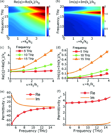
Figure 2: Contour plots of restored (a) $Re[q(\omega,\kappa)]$ and (b) $Im[q(\omega,\kappa)]$ for a graphene stripe of $w=80$nm show absence of resonances at low frequencies, but a resonance at $f=17$ THz. Looking at the $q(\kappa)$ for certain frequencies (5, 10, 15 THz) we observe the flat $Re[q(\kappa)]$ dependence (c) and smaller losses (d) for the frequency. Effective radial permittivity $\varepsilon_{r}$(e) shows the Drude-like behavior, while azimuthal permittivity $\varepsilon_{\theta}$ (f) is positive with small losses.

In order to select the optimal geometrical design, we investigated the dependence of the wire medium properties on the stripe width (see Fig. 3) starting from no graphene ($w=0$) to a full graphene coverage ($w=200$ nm). As expected, in the absence of graphene we restore a constant refractive index $n_{D}=1.53$ (Fig. 3a) with no losses (Fig. 3b) and permittivities $\varepsilon_{r}=\varepsilon_{\theta}=n_{D}^{2}$ (Fig. 3c,d), while for the full graphene coverage a typical Drude metal-like behavior is observed for permittivities $\varepsilon_{r}=\varepsilon_{\theta}$. Changing the width from $w=80$ nm, which we discussed above, to $w=160$ nm we observe larger values of $Re(q)$ for the normal propagation $\kappa=0$ (see Fig. 3a) (and consequently worse coupling efficiency), larger losses and red shift of the resonance to $f=13$ THz (Fig. 3b) and larger negative permittivity $\varepsilon_{r}$ (Fig. 3c). After examining several widths we selected for the hyperlens demonstration the width $w=40$ nm (not shown in Fig. 3) and the frequency 6 THz.

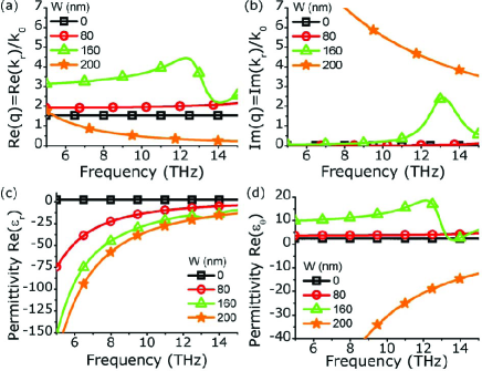
Figure 3: Comparison of the properties of the graphene wire medium for various stripe widths (0, 80, 160 and 200 nm). The radial wavevector shows larger values of (a) $Re(q)$ (that means worse coupling to the surrounding medium) and (b) $Im(q)$ (larger losses) for $w=160$ nm compared to the width $w=80$ nm. Also, a ”more metallic” Drude behaviour of $\varepsilon_{r}$ (c) and higher azimuthal permittivity $\varepsilon_{\theta}$ (d) nm is observed for $w=160$. The absence of graphene ($w=0$) and full coverage ($w=200$ nm) show fully dielectric and Drude-like behaviours, respectively.

To check the suitability of the effective medium approach we simulated in the CST (time domain) the full-size 3D hyperlens made of graphene stripes embedded into dielectric ($n_{D}=1.53$). One layer of the hyperlens is shown in the Fig. 4(a). The input and output periods, widths and radii were chosen as $P_{\rm{in}}=200$ nm, $P_{\rm{out}}=600$ nm, $W_{\rm{in}}=40$ nm, $W_{\rm{out}}=120$ nm, $R_{\rm{in}}=15.12\mu$m and $R_{\rm{out}}=45.36\mu$m, respectively. The radii are selected to satisfy the Fabry-Perot resonant condition (2). The layers of structured graphene are assumed to be periodic in the direction perpendicular to the image plane (period $a_{y}=50$ nm). We should note that the specified sizes are realistic for fabrication. Multiple graphene layers separated with a dielectric can be made up to the size of 30 inches Bae et al. (2010). Structuring of multiple graphene-dielectric layers structure can be done with focused ion beam milling or electron beam lithography.

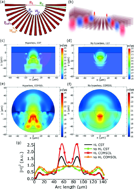
Figure 4: (a) A single structured graphene layer that constitutes the hyperlens. (b) An artistic 3D view of the hyperlens in action: the image of two line sources is magnified with the hyperlens. Full size 3D CST simulation of the hyperlens (c) in action and no hyperlens (d), when two magnetic line sources separated by $\lambda_{0}/5=10\mu$m are emitting TM polarized waves (magnetic field perpendicular to the plane of image). The CST results are in a good agreement with equivalent 2D COMSOL simulations of the hyperlens (e) and no hyperlens (f). Comparison of the intensity distribution at the output interface of the hyperlens (g) confirms that the images are well resolved.

Now we show the hyperlens in action when being excited with two sources (line magnetic currents) in vacuum separated with distance $\delta=\lambda_{0}/5=10\mu$m (see the artistic 3D view of the hyperlens in work in Fig. 4b). In the presence of the hyperlens two sources are well resolved at the output interface as two peaks separated with $30\mu$m (Fig. 4c) delivering the magnification $M=R_{2}/R_{1}=3$, while in case of the homogenous dielectric cylinder (no graphene wires) we observe a single spot (Fig. 4d).

Then we compared the CST results with an equivalent 2D hyperlens simulation in COMSOL COM (scattering boundary conditions) with homogenized permittivities $\varepsilon_{r}=-20.1+8.5i$, $\varepsilon_{\theta}=2.73+0.0029i$. The COMSOL results with (Fig. 4e) and without the hyperlens (Fig. 4f) are in a good agreement with the CST results. A comparison between them is shown in Fig. 4g where the wave intensity at the output interface of the lens is presented. The intensity of the peaks in the presence of the hyperlens is larger than in its absence, due to redistribution of the power. The intensity simulated with the CST is smaller compared to COMSOL that is caused by the coarser spatial discretization of the tapered wires with a staircase numerical mesh in the CST. In both types of simulations the peaks are well resolved according to the Rayleigh criterion. The 2D COMSOL simulation, however, took several minutes versus the 3-days long 3D CST modeling.

By making a hyperlens with larger radius $R_{2}$ one can achieve a larger magnification. For example, selecting $R_{2}=10R_{1}$ gives the magnification $M=10$, so two point sources with separation $\delta=10\mu$m are imaged to $100\mu$m (see Fig. 5a) and then can be resolved with a conventional THz camera.

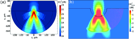
Figure 5: (a) A thicker hyperlens with $R_{2}=10R_{1}$ magnifies two subwavelength sources until the images can be captured with a conventional THz imaging system. (b) Tracing the maximum of the broadband THz transient pulse shows that the hyperlens works in the range of frequencies around 6 THz.

It is important to test the device performance under the pulse excitation. In the conventional THz time domain spectroscopy setupJepsen et al. (2011) (THz-TDS), a very short (single cycle or even shorter) THz pulse is generated. Experimentally testing the hyperlens in the real THz-TDS would mean shining the short (and therefore broadband in frequency) transient pulse and then scanning with the THz near-field microscope and collecting the time-dependent signal at the output. We did a similar simulation in CST, exciting 2 sources with the Gaussian pulse (central frequency $f_{c}=6$ THz, FWHM = 12 THz), recording the field with the time monitor and then imaging the maximal field in each point during the simulation time (Fig. 5b). Since the graphene hyperlens is not based on a resonant medium, it can operate in an extended range of frequencies and two sources are well magnified and resolved (Fig. 5b).

Due to reciprocity the hyperlens can be used not only for imaging, but also for THz power concentration into a small volume. We wish to note that the employment of metal for the considered hyperlens design is hardly possible. In order to obtain the same conductivity of the unit cell as of the regarded graphene stripes, the cross-section of the metallic wire (for example, silver Laman and Grischkowsky (2008)) has to be of $2\mu$m². Fabricating and arranging so thin and long metallic wires into the required pattern is beyond the possibilities of the current nanofabrication technologies. We should emphasize that the scaling up the metallic wires together with the unit cell is not possible, since the period of the hyperlens should be subwavelength even for the higher-order spatial harmonics. Another important advantage of the graphene hyperlens compared to the metal based one is its tunability by the graphene chemical potential change. Thus it is possible to make the device reconfigurable and to resolve subwavelength features or concentrate THz pulses on demand.

In conclusion, we have shown that structured graphene layers embedded into dielectric (graphene wire medium) can be used to create a hyperlens. We have proposed the realistic geometrical design for the hyperlens for the THz radiation and proved that it can resolve two line sources separated by a distance $\lambda_{0}/5$. We also showed that time-consuming 3D simulations are in a good agreement with the quick homogenized 2D hyperlens modeling, which simplifies the hyperlens engineering.