Shear surface waves in phononic crystals

Abstract

Existence of shear horizontal (SH) surface waves in 2D-periodic phononic crystals with an asymmetric depth-dependent profile is theoretically reported. Examples of dispersion spectra with band gaps for subsonic and supersonic SH surface waves are demonstrated. The link between the effective (quasistatic) speeds of the SH bulk and surface waves is established. Calculation and analysis is based on the integral form of projector on the subspace of evanescent modes which means no need for their explicit finding. This new method can be extended to the vector waves and the 3D case.

I Introduction

Emergence of phononic crystals has reinforced the interest to surface waves in periodic media and heighten the need for efficient methods of calculating their dispersion branches. Considerable work has been done for solid structures which are periodic along the surface but uniform along the depth direction. The latter implies pure exponential dependence on depth coordinate and thus facilitates the plane-wave expansion (PWE) which acts on the surface coordinates only. Applying PWE to the wave equation provides a formally infinite algebraic system whose truncation enables explicit finding of the evanescent (decreasing with the depth) modes which are then used to satisfy another formally infinite system obtained by PWE of the boundary condition on the free surface. The above two-step PWE procedure was first implemented for Rayleigh waves in a periodic structure of layers normal to the surface DMW and then extended to 2D phononic crystals composed of elastic TT ; WHL and piezoelectric LWBK ; WHH rods normal to the surface. Surface waves in such periodic structures uniform along the depth direction were also calculated by FDTD SW ; TTT and wavelet YW methods.

By contrast, much fewer results for surface waves are available in the alternative case of structures which are periodic both along the surface and the depth coordinates, such as rods parallel to the surface. We have found only three references reporting calculation of surface-wave dispersion in depth-dependent phononic crystals MR ; Z-K ; LHOA , both papers using pure numerical means (namely, the supercell approximation approach). One of the apparent difficulties due to depth dependence is a numerically more involved procedure of identifying of evanescent wave harmonics. Note that the so-called extended PWE was suggested as a tool for this purpose LABK ; RSG ; RGVHHGRSP , but its application to the surface wave problem in hand has not been envisaged.

The present paper pursues two objectives. The first is a new method for calculating surface wave branches in depth-dependent phononic crystals. The main point and advantage of the method is that the dispersion equation is expressed in terms of the projector on the subspace of evanescent modes and this projector is defined directly from the material coefficients expanded in Fourier series in surface coordinate(s), without a need to solve for partial modes and to explicitly sort out the evanescent ones. In principle, the proposed method can be used for general case of vector waves in arbitrary periodic solid structures, but here it is applied to shear horizontal (SH) waves. Study of SH surface waves in 2D phononic crystals is the second objective of the paper. This is an interesting problem of its own right. It is well-known that the SH surface (localised) waves in 1D periodically layered half-space can or cannot exist if the layers are parallel or orthogonal to the surface, respectively. At the same time, we are unaware of results providing explicit evidence of SH surface waves in 2D periodic structures. Uncoupling of SH modes implies 2D depth-dependent structures, the case which defies PWE and was treated by the supercell method in MR ; Z-K ; LHOA ; however, the surface waves with SH polarization appear to be beyond the scope of this method. As pointed out in MR , the difficulty came from the fact that the SH surface waves could occur only if the unit cell was asymmetric but this made the supercell method ”insufficient or inappropriate”. In contrast, asymmetry of periodic profile causes no inconvenience for our method. By its means we demonstrate examples of subsonic and supersonic dispersion branches of SH surface waves in 2D phononic crystals.

The paper is organised as follows. The statement of the problem is outlined in Sec. II. The method for calculating the surface-wave spectrum is developed in Sec. III. Its application is exemplified in Sec. IV. Properties of the SH surface waves and the generalization to 3D case are discussed in Sec. V. Main findings are summarized in Sec. VI.

II Statement of the problem

Consider SH surface waves in a 2D periodic half-space $\{{\bf x}=(x_{1},x_{2}):x_{2}\geq 0\}$ with a traction-free surface $x_{2}=0$. The problem consists of the wave equation complemented by the boundary and radiation conditions, namely

$$\begin{cases}\partial_{1}(\mu\partial_{1}v)+\partial_{2}(\mu\partial_{2}v)=-\rho\omega^{2}v,\\ \partial_{2}v|_{x_{2}=0}=0,\ \ \lim\limits_{x_{2}\to\infty}v=0,\end{cases}$$ (1)

where $\partial_{i}\equiv\partial/\partial x_{i}$ and the shear coefficient $\mu({\bf x})$ and density $\rho({\bf x})$ are ${\bf 1}$-periodic in $x_{1}$ and $x_{2}$. (All subsequent results remain explicitly valid for rectangular lattices and can be adjusted straightforwardly to the case of oblique lattices.) Applying PWE in surface coordinate $x_{1}$, i.e. inserting 1D Floquet condition along with the Fourier expansion

$$v({\bf x})=u({\bf x})e^{ik_{1}x_{1}}\ \ {\rm with}\ u\ {\rm periodic\ in\ }x_{1},$$

$$h=\sum_{m}\widehat{h}_{m}(x_{2})e^{2\pi imx_{1}}\ \ {\rm for}\ \ h=u,\mu,\rho,$$ (2)

casts (1) in the form

$$\begin{cases}(\boldsymbol{\partial}+k_{1})\boldsymbol{\mu}(\boldsymbol{\partial}+k_{1}){\bf u}-\partial_{2}(\boldsymbol{\mu}\partial_{2}{\bf u})=\boldsymbol{\rho}\omega^{2}{\bf u},\\ \partial_{2}{\bf u}|_{x_{2}=0}={\bf 0},\ \ \lim\limits_{x_{2}\to\infty}{\bf u}={\bf 0}\end{cases}$$ (3)

with

$${\bf h}(x_{2})=(\widehat{h}_{n-m}(x_{2}))\ \ {\rm for}\ \ h=\mu,\rho,$$

$$\boldsymbol{\partial}=2\pi(m\delta_{n-m}),\ \ {\bf u}(x_{2})=(\widehat{u}_{m}(x_{2})),\ \ n,m\in{\mathbb{Z}}.$$ (4)

For practical use, we assume all objects in (II) to be of finite dimension. Equation (3) can be rewritten as

$$\begin{cases}\boldsymbol{\eta}^{\prime}={\bf Q}\boldsymbol{\eta},\\ \boldsymbol{\eta}(0)=({\bf u}_{0}\ {\bf 0})^{\top},\ \ \lim\limits_{x_{2}\to\infty}\boldsymbol{\eta}(x_{2})={\bf 0},\end{cases}$$ (5)

where ${}^{\prime}\equiv\partial_{2}$ and

$$\boldsymbol{\eta}=\begin{pmatrix}{\bf u}\\ \boldsymbol{\mu}{\bf u}^{\prime}\end{pmatrix},\ \ {\bf Q}=\begin{pmatrix}{\bf 0}&\boldsymbol{\mu}^{-1}\\ (\boldsymbol{\partial}+k_{1})\boldsymbol{\mu}(\boldsymbol{\partial}+k_{1})-\omega^{2}\boldsymbol{\rho}&{\bf 0}\end{pmatrix}.$$ (6)

The solution to $\boldsymbol{\eta}^{\prime}={\bf Q}\boldsymbol{\eta}$ with initial data $\boldsymbol{\eta}(0)$ is

$$\boldsymbol{\eta}(x_{2})={\bf M}(x_{2})\boldsymbol{\eta}(0)\ \ {\rm with}\ \ {\bf M}(x_{2})=\widehat{\int_{0}^{x_{2}}}({\bf I}+{\bf Q}dx_{2}),$$ (7)

where $\widehat{\int}$ is the multiplicative integral and ${\bf I}$ is identity matrix. Introduce the monodromy matrix

$${\bf M}_{0}={\bf M}_{0}(\omega,k_{1})\equiv{\bf M}(1)$$ (8)

and let $q$ and ${\bf w}$ be its eigenvalues and eigenvectors. Taking some ${\bf w}$ as initial data in (7) defines the Floquet mode $\boldsymbol{\eta}(x_{2})={\bf M}[x_{2},0]{\bf w}=q^{n}{\bf M}[x_{2}-n,0]{\bf w}$ (where $n=\lfloor x_{2}\rfloor$), which is either propagating or increasing or decreasing at $x_{2}\to\infty$ depending on the absolute value of the eigenvalue $q$ corresponding to ${\bf w}$. In the case of propagating modes ($|q|=1$), the spectrum $\omega=\omega({\bf k})$ (${\bf k}=(k_{1},k_{2})\in{\mathbb{R}}^{2}$) defined by the equation $q(\omega,k_{1})=e^{ik_{2}}$ is called the Floquet spectrum.

III Projector-based method for calculating surface wave spectrum

1. Projectors. Partition the eigenspace of ${\bf M}_{0}$ into the folowing subspaces:

$$\begin{cases}{\mathcal{L}}_{\rm d}=\langle{\bf w}:\ {\bf M}_{0}{\bf w}=q{\bf w},\ |q|<1\rangle,\\ {\mathcal{L}}_{\rm p}=\langle{\bf w}:\ {\bf M}_{0}{\bf w}=q{\bf w},\ |q|=1\rangle,\\ {\mathcal{L}}_{\rm i}=\langle{\bf w}:\ {\bf M}_{0}{\bf w}=q{\bf w},\ |q|>1\rangle,\end{cases}$$ (9)

where $\langle...\rangle$ means a span. Taking (7) with $\boldsymbol{\eta}(0)$ from ${\mathcal{L}}_{\rm d}$ or ${\mathcal{L}}_{\rm p}$ or ${\mathcal{L}}_{\rm i}$ leads to decreasing or propagating or increasing solution $\boldsymbol{\eta}(x_{1})$, respectively. The projectors ${\bf P}_{\alpha}$ on ${\mathcal{L}}_{\alpha}$ ($\alpha={\rm d},{\rm p},{\rm i}$), i.e.

$${\bf P}_{\alpha}{\bf w}=\begin{cases}{\bf w},&{\bf w}\in{\mathcal{L}}_{\alpha},\\ {\bf 0},&{\bf w}\not\in{\mathcal{L}}_{\alpha},\end{cases}$$ (10)

can be defined by the formulas

$$\begin{cases}{\bf P}_{\rm d}=\frac{1}{2\pi i}\int\limits_{|z|=1-0}(z{\bf I}-{\bf M}_{0})^{-1}dz,\\ {\bf P}_{\rm p}=\frac{1}{2\pi i}(\int\limits_{|z|=1+0}-\int\limits_{|z|=1-0})(z{\bf I}-{\bf M}_{0})^{-1}dz,\\ {\bf P}_{\rm i}={\bf I}-\frac{1}{2\pi i}\int\limits_{|z|=1+0}(z{\bf I}-{\bf M}_{0})^{-1}dz.\end{cases}$$ (11)

By definition

$${\bf P}_{\rm d}+{\bf P}_{\rm p}+{\bf P}_{\rm i}={\bf I}.$$ (12)

Note that both ${\bf P}_{\rm p}$ and ${\bf P}_{\rm i}$ can be expressed in terms of ${\bf P}_{\rm d}$, see (V).

2. Dispersion equation. The surface wave problem (5) is equivalent to any one of the following conditions

$$\exists{\bf u}_{0} \neq {\bf 0}:\ \ \begin{pmatrix}{\bf u}_{0}\\ {\bf 0}\end{pmatrix}\in{\mathcal{L}}_{\rm d}\ \Leftrightarrow$$ (13)

$$\exists{\bf u}_{0} \neq {\bf 0}:\ \ {\bf P}_{\rm d}\begin{pmatrix}{\bf u}_{0}\\ {\bf 0}\end{pmatrix}=\begin{pmatrix}{\bf u}_{0}\\ {\bf 0}\end{pmatrix}\ \Leftrightarrow$$ (14)

$$\exists{\bf u}_{0} \neq {\bf 0}:\ {\bf P}_{{\rm d}3}{\bf u}_{0}={\bf 0},\ \ {\bf P}_{{\rm d}1}{\bf u}_{0}={\bf u}_{0},$$ (15)

where

$${\bf P}_{\rm d}=\begin{pmatrix}{\bf P}_{{\rm d}1}&{\bf P}_{{\rm d}2}\\ {\bf P}_{{\rm d}3}&{\bf P}_{{\rm d}4}\end{pmatrix}.$$ (16)

According to (15), the surface wave spectrum $\omega_{\rm saw}(k_{1})$ can be defined by the dispersion equation

$$D_{\rm saw}(\omega,k_{1})\equiv\mathop{\mathrm{det}}\nolimits(({\bf P}_{{\rm d}1}-{\bf I})^{*}({\bf P}_{{\rm d}1}-{\bf I})+{\bf P}_{{\rm d}3}^{*}{\bf P}_{{\rm d}3})=0,$$ (17)

where ^∗ means Hermitian conjugation.

3. Projection of the Floquet spectrum on the plane $(\omega,k_{1})$. Recall that the Floquet spectrum $\omega({\bf k})$ can be determined by the equation

$$\exists{\bf w}\neq{\bf 0}:\ \ {\bf M}_{0}(\omega,k_{1}){\bf w}=e^{ik_{2}}{\bf w}.$$ (18)

Introduce the multiplicity of the projection of the Floquet spectrum on the plane $(\omega,k_{1})$

$$N_{\rm p}(\omega,k_{1})=\#\{k_{2}\in{\mathbb{R}}:\ \omega({\bf k})=\omega\},$$ (19)

which indicates the number of propagating modes. By (9), (10) and (18), it can be evaluated as

$$N_{\rm p}(\omega,k_{1})=\mathop{\mathrm{dim}}\nolimits{\mathcal{L}}_{\rm p}={\rm Trace}\ {\bf P}_{\rm p}.$$ (20)

By definition, $N_{\rm p}$ is a piecewise constant function with integer even values. Denote the boundaries of areas where $N_{\rm p}$ takes the same value by $\omega_{\rm tr}(k_{1})$ and call them transonic curves. These curves coincide with the projection of local extrema of Floquet branches $\omega({\bf k})$ on the plane $(\omega,k_{1})$. The areas of $(\omega,k_{1})$-plane where $N_{\rm p}\neq 0(\Leftrightarrow{\bf P}_{\rm p}\neq{\bf 0})$ and $N_{\rm p}=0(\Leftrightarrow{\bf P}_{\rm p}={\bf 0})$ will be referred to as propagative and non-propagative domains, respectively. The whole subsonic range $\{(\omega,k_{1}):\ \omega<\omega_{{\rm tr},1}(k_{1})=\min_{k_{2}}\omega({\bf k})\}$, i.e. the part of the plane $(\omega,k_{1})$ below the minimal frequency of the Floquet spectrum $\omega({\bf k})$, is always non-propagative by definition. Owing to existence of spectral gaps in $\omega({\bf k})$, the non-propagative domains may also arise in the supersonic range, i.e. above $\omega_{{\rm tr},1}(k_{1})$.

4. Refined procedure in the non-propagative domains. Consider a non-propagative domain $N_{\rm p}(\omega,k_{1})=0$. According to (15) and the identity ${\bf P}_{\rm d}+{\bf P}_{\rm i}={\bf I}$ (see (12)), any root $(\omega,k_{1})$ of the equation

$$D_{{\rm d}3}(\omega,k_{1})\equiv\mathop{\mathrm{det}}\nolimits{\bf P}_{{\rm d}3}=0$$ (21)

corresponds to a surface-wave solution $\omega_{\rm saw}(k_{1})$ (see (13)) or a nonphysical solution $\omega_{\rm i}(k_{1})$ which contains of increasing modes (i.e. $\begin{pmatrix}{\bf u}_{0}&{\bf 0}\end{pmatrix}^{\top}\in{\mathcal{L}}_{\rm i}$ instead of (13)). Note that $D_{{\rm d}3}(\omega,k_{1})$ is a real function for real arguments, since ${\bf P}_{{\rm d}3}$ is a self-adjoint matrix at $N_{\rm p}=0$, see (39). Unlike non-negative $D_{\rm saw}$ in (17), the function $D_{{\rm d}3}$ generally changes sign at its zeroes. Thus seeking the surface waves in non-propagative domains, it is convenient to use (21) alongside (17): the former verifies that a ”numerical zero” is not a deep but nonzero minimum and the latter checks out whether this zero defines a surface wave rather than a non-physical wave. Note that surface waves can also be identified by using (21) along with the condition ${\bf P}_{{\rm d}1}{\bf u}_{0}\neq{\bf 0}$, where ${\bf u}_{0}$ is defined by ${\bf P}_{{\rm d}3}{\bf u}_{0}={\bf 0}$.

In the propagative domains $N_{\rm p}(\omega,k_{1})\neq 0$, due to $\mathop{\mathrm{rank}}\limits{\bf P}_{\rm d}=\mathop{\mathrm{rank}}\limits{\bf P}_{\rm i}$ and ${\bf P}_{\rm p}\neq{\bf 0}$ it follows from (12) that $\mathop{\mathrm{rank}}\limits{\bf P}_{{\rm d}3}\leq\mathop{\mathrm{rank}}\limits{\bf P}_{\rm d}<\frac{1}{2}\mathop{\mathrm{rank}}\limits{\bf I}=\mathop{\mathrm{dim}}\nolimits{\bf P}_{{\rm d}3}$. Therefore (21) is an identity in propagative domains and so it cannot be used for defining $\omega_{\rm saw}(k_{1})$ in propagative domains.

5. Calculation of projectors. Equation (11) defines the projector $\mathbf{P}_{\mathrm{d}}$ as an integral of the resolvent $\mathbf{R}_{z0}=(z{\bf I}-{\bf M}_{0})^{-1}.$ One way to obtain $\mathbf{R}_{z0}$ is to compute $\mathbf{M}_{0}$ defined by (7). However, computing $\mathbf{M}_{0}$ of large algebraic dimension $2d\times 2d$ (which means taking into account many members of the Fourier series, see (II)) is numerically troublesome because some of its components grow exponentially as $d$ increases. On the other hand, components of $\mathbf{R}_{z0}$ can grow in general only as fast as linearly in $d$. Therefore it is numerically adavantageous to calculate $\mathbf{R}_{z0}$ directly rather than via $\mathbf{M}_{0}$.

Denote

$$\mathbf{R}_{\alpha}(x_{2})=(\alpha{\bf I}-{\bf M}(x_{2}))^{-1}$$ (22)

where $\alpha$ is some fixed constant which does not belong to the spectrum of $\mathbf{M}$. As a solution to (5), $\mathbf{M}$ satisfies the linear differential equation with initial data

$$\begin{cases}\mathbf{M}^{\prime}(x_{2})=\mathbf{Q}(x_{2})\mathbf{M}(x_{2}),\\ \mathbf{M}(0)=\mathbf{I},\end{cases}$$ (23)

from which it follows that $\mathbf{R}_{\alpha}$ satisfies the Ricatti equation

$$\begin{cases}{\bf R}_{\alpha}^{\prime}(x_{2})={\bf R}_{\alpha}(x_{2}){\bf Q}(x_{2})(\alpha{\bf R}_{\alpha}(x_{2})-{\bf I}),\\ {\bf R}_{\alpha}(0)=(\alpha-1)^{-1}{\bf I}.\end{cases}$$ (24)

Numerical integration of (24) provides the value $\mathbf{R}_{\alpha 0}={\bf R}_{\alpha}(1)$ for a given $\alpha$. Once it is found, the identity

$${\bf R}_{z0}={\bf R}_{\alpha 0}({\bf I}+(z-\alpha){\bf R}_{\alpha 0})^{-1}$$ (25)

yields $\mathbf{R}_{z0}$ with varying $z$ as required in (11). Thus combining (11) and (25) defines the projector $\mathbf{P}_{\mathrm{d}}$ in the following specialized form

$${\bf P}_{\rm d}=\frac{{\bf R}_{\alpha 0}}{2\pi}\int_{0}^{2\pi}re^{i\varphi}({\bf I}+(re^{i\varphi}-\alpha){\bf R}_{\alpha 0})^{-1}d\varphi$$ (26)

with $r<1$ sufficiently close to $1$. Two other projectors $\mathbf{P}_{\mathrm{i}}$ and $\mathbf{P}_{\mathrm{p}}$ are expressed via $\mathbf{P}_{\mathrm{d}},$ see (V).

In numerical implementation, we used the fourth order Runge-Kutta method for calculating $\mathbf{R}_{\alpha 0}$ from (24) where $\alpha\in{\mathbb{C}}$ has being chosen randomly anew for each next calculation point $(\omega,k_{1})$. It is recommended to avoid taking $\alpha$ near the real axis or the unit circle (we used $\alpha\in[-6,-3]\times[3i,6i]$). The Chebyshev method was employed for evaluating (26) where we took $r=0.99$. Dealing with Eqs. (17) and (21) it is convenient to use ’normalised’ functions

$$D_{\mathrm{saw}}(\omega,k_{1}) = \lambda_{\min}(\omega,k_{1}),$$

$$D_{\mathrm{d}3}(\omega,k_{1}) = \mathop{\mathrm{det}}\nolimits(\mathbf{P}_{\mathrm{d}3}^{-1}(0,k_{1})\mathbf{P}_{\mathrm{d}3}(\omega,k_{1})),$$ (27)

where $\lambda_{\min}$ is the minimal eigenvalue of the self-adjoint non-negative operator whose determinant is taken in (17).

IV Examples

1. Stiff cylinders in a soft matrix. Assume an epoxy matrix with a periodic structure of steel cylindrical bars parallel to the free surface $x_{2}=0$. The material constants are $\rho=1.14\ {\rm g/cm}^{3}$, $\mu=1.48\ {\rm GPa}$ for epoxy and $\rho=7.8\ {\rm g/cm}^{3}$, $\mu=80\ {\rm GPa}$ for steel. Let the steel bars form a rectangular lattice with the horizontal and vertical periods $a_{1}:a_{2}=1:2$, and the radius of bars be $0.45a_{1}$ (in the following, $a_{1}\equiv 1$ and $k_{1}a_{1}\equiv k_{1}$, $\omega a_{1}\equiv\omega$ in units ${\rm mm/\upmu s}$). For obtaining SH surface waves, it is necessary that the unit cell is asymmetric about the horizontal midplane (see Sec. V.1). We shall consider two interrelated types of structures which are reciprocal to each other in the sense that their unit cells pass into one another by means of reflection about the horizontal midplane, see Fig. 1. Note that the unit cell of the structure (a) is ’faster’ on the top than on the bottom, hence vice versa for the structure (b). Figure 2 demonstrates that the two reciprocal structures are characterized at fixed $(\omega,k_{1})$ by the same number $N_{\mathrm{p}}$ of propagating modes, whereas the frequency $\omega_{\mathrm{saw}}$ of surface-wave solutions for the configuration (b) is the frequency $\omega_{\mathrm{i}}$ of non-physical solutions for the configuration (a). A general proof for this feature is given in Sec. V.2.

The surface-wave dispersion branches $\omega_{\mathrm{saw}}(k_{1})$ for the structure (b) are shown in Fig. 3. For this calculation, we used $d=17$ terms of the Fourier series (II). Numerical data clearly show that there exists a subsonic branch $\omega_{\mathrm{saw},1}$ below the first transonic curve $\omega_{\mathrm{tr},1}$, though their relative difference is only of the order of $1\%$. Subsonic and supersonic surface waves occurring in the non-propagative domains ($N_{\mathrm{p}}=0$) are defined by common zeros of Eqs. (17) and (21). In propagative domains ($N_{\mathrm{p}}\neq 0$), a surface wave is defined only by (17) and is therefore associated, in the numerical context, with a minimum which tends to zero with growing number $d$ of terms of Fourier series. The surface-wave branches shown within the upper propagative domain in Fig. 3 yield the value of $D_{\mathrm{saw}}=\lambda_{\min}$ (see (III)) of about $10^{-3}$.

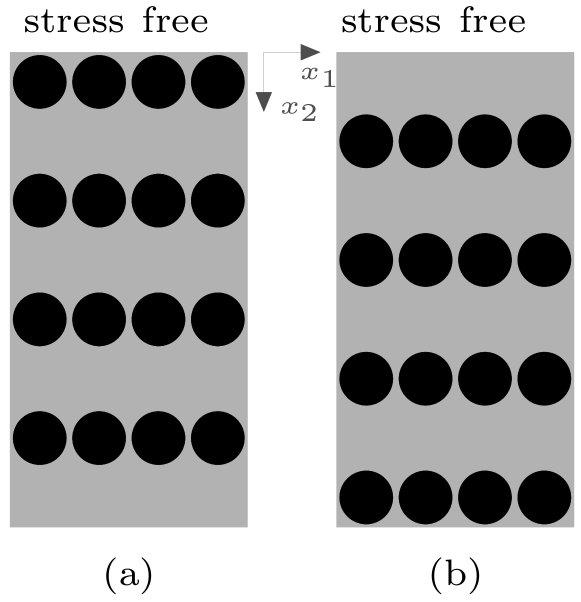
Figure 1: Reciprocal configurations of a periodic structure of steel cylinders in epoxy matrix.

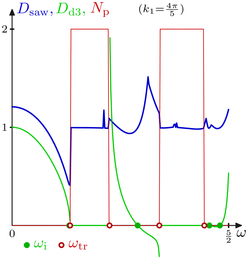
(a)

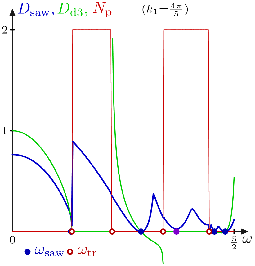
(b)

Figure 2: (color online) The function $N_{\mathrm{p}}(\omega)$ (see (20)) and the normalized functions $D_{\mathrm{saw}}(\omega)$ and $\ D_{\mathrm{d}3}(\omega)$ (see (III)) calculated at fixed $k_{1}=4\pi/5$ for the reciprocal structures (a) and (b) of Fig. 1, respectively. The curves $D_{\mathrm{d}3}$ and $N_{\mathrm{p}}$ do not change on passing from one configuration to another, see (31). Zeros of $D_{\mathrm{d}3}$ at $N_{\mathrm{p}}=0$ are surface-wave solutions $\omega_{\mathrm{saw}}$ when they coincide with zeros of $D_{\mathrm{saw}}$, otherwise they are non-physical solutions $\omega_{\mathrm{i}}$.

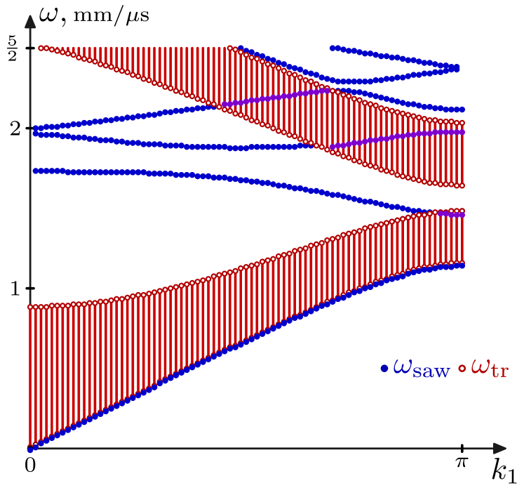
Figure 3: Surface-wave dispersion branches $\omega_{\mathrm{saw}}(k_{1})$ and transonic curves $\omega_{\mathrm{tr}}(k_{1})$ for the structure displayed in Fig. 1b. Blank and hatched areas are the non-propagative and propagative domains, respectively.

2. Perturbation of 1D-periodic structure. In order to illuminate formation of surface-wave spectrum, let us think of a vertically periodic stack of equidistant epoxy and iron layers (Fig. 4a) and then assume that each epoxy layer contains narrow lead plates embedded periodically along the horizontal direction (Fig. 4b). The material constants are $\rho=116\ {\rm g/cm}^{3}$, $\mu=7.88\ {\rm GPa}$ for Fe and $\rho=14.9\ {\rm g/cm}^{3}$, $\mu=11.6\ {\rm GPa}$ for Pb. Taking the ratio of the horizontal to vertical periods $a_{1}:a_{2}=1:3$ for both cases and applying the calculation procedure of Sec. III leads to the spectra shown in Figs. 5a and 5b, respectively. It is clearly seen that introducing horizontal periodicity creates band gaps at the edge and inside of the Brillouin zone.

Figure 4: Periodic structure of epoxy and iron layers (a) and a similar structure but with lead baffles in epoxy (b). Lead to epoxy volume fraction is $1:9$.

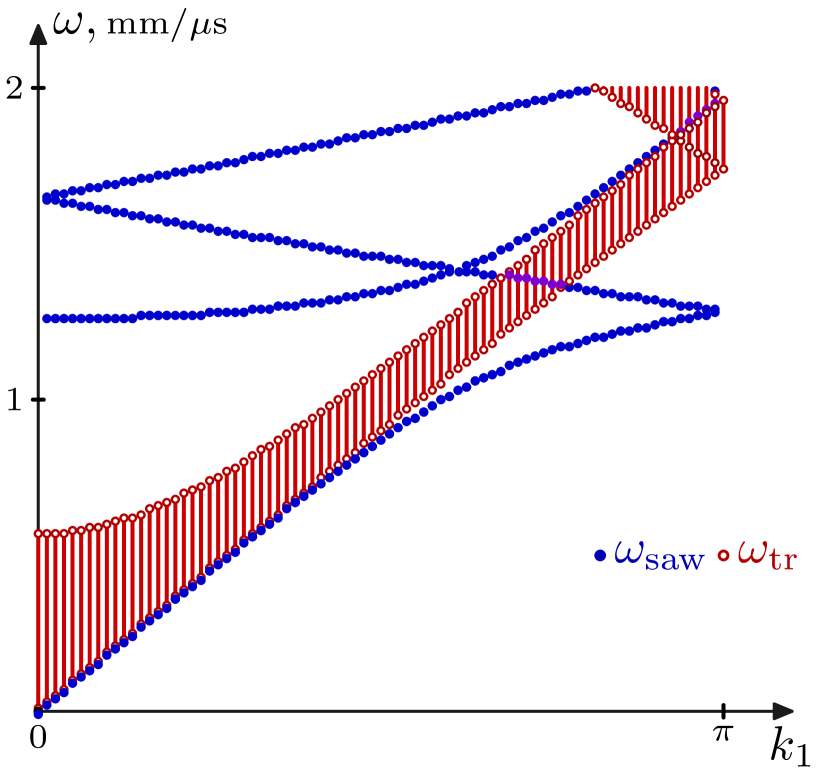
(a)

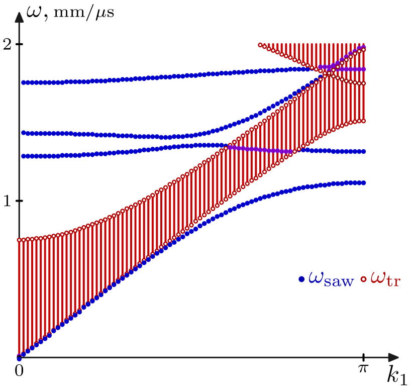
(b)

Figure 5: Surface-wave dispersion spectra $\omega_{\mathrm{saw}}(k_{1})$ (a) and (b) for the structures displayed in Fig. 4a and 4b, respectively. Notations are the same as in Fig. 3.

V Discussion

1. Reciprocity property for SH surface waves. Given periodic functions $\mu(\mathbf{x})$ and $\rho(\mathbf{x})$ of $\mathbf{x}=(x_{1},x_{2})\in{\mathbb{R}}^{2}$, let us mentally cut the space into two halves by the plane $x_{2}=0$ and turn the half-space $x_{2}\leq 0$ upside down. Thus we obtain two models of a half-space $x_{2}\geq 0$: one with the profile $\mu(\mathbf{x})$, $\rho(\mathbf{x})$ and another with the reciprocal profile $\widetilde{\mu}(\mathbf{x})=\mu(x_{1},-x_{2})$, $\widetilde{\rho}(\mathbf{x})=\rho(x_{1},-x_{2})$. Consider the relation between the properties for a direct and reciprocal profiles (the objects constructed from $\widetilde{\mu}$, $\widetilde{\rho}$ will be labeled by a tilde).

By (7) and the definition of multiplicative integral,

$$\begin{array}[]{c}\mathbf{M}_{0}^{-1}=\lim\limits_{N\to\infty}\prod\limits_{j=N}^{1}\biggl{(}\mathbf{I}-\frac{1}{N}\mathbf{Q}\left(\frac{N-j}{N}\right)\biggr{)}\\ =\lim\limits_{N\rightarrow\infty}\prod\limits_{j=N}^{1}\biggl{(}\mathbf{I}-\frac{1}{N}\widetilde{\mathbf{Q}}\left(\frac{j}{N}\right)\biggr{)}=\mathbf{S}\widetilde{\mathbf{M}}_{0}\mathbf{S}\\ {\rm with}\ \ {\bf S}={\bf S}^{-1}=\begin{pmatrix}\mathbf{I}&\mathbf{0}\\ \mathbf{0}&-\mathbf{I}\end{pmatrix},\end{array}$$ (28)

where we used that $\mathbf{S}\widetilde{\mathbf{Q}}\mathbf{S=-}\widetilde{\mathbf{Q}}$ since $\widetilde{\mathbf{Q}}$ has zero diagonal blocks, see (6). According to (28), the eigen-subspaces and projectors for direct and reciprocal profiles are related as follows:

$$\begin{cases}\widetilde{\mathcal{L}}_{\rm d}={\bf S}{\mathcal{L}}_{\rm i},&\widetilde{\bf P}_{\rm d}={\bf S}{\bf P}_{\rm i}{\bf S},\\ \widetilde{\mathcal{L}}_{\rm i}={\bf S}{\mathcal{L}}_{\rm d},&\widetilde{\bf P}_{\rm i}={\bf S}{\bf P}_{\rm d}{\bf S},\\ \widetilde{\mathcal{L}}_{\rm p}={\bf S}{\mathcal{L}}_{\rm p},&\widetilde{\bf P}_{\rm p}={\bf S}{\bf P}_{\rm p}{\bf S}.\end{cases}$$ (29)

Using a similar to (16) notation for the blocks of ${\bf P}_{\rm i}$, introduce the equation

$$D_{\rm i}(\omega,k_{1})\equiv\mathop{\mathrm{det}}\nolimits(({\bf P}_{{\rm i}1}-{\bf I})^{*}({\bf P}_{{\rm i}1}-{\bf I})+{\bf P}_{{\rm i}3}^{*}{\bf P}_{{\rm i}3})=0,$$ (30)

whose solutions $\omega_{\rm i}(k_{1})$ describe non-physical waves which satisfy the stress-free condition but consist of increasing modes. From (29), with reference to (17), (30) and (20),

$$D_{\mathrm{saw}}=\widetilde{D}_{\mathrm{i}},\ D_{\mathrm{i}}=\widetilde{D}_{\mathrm{saw}},\ D_{{\rm d}3}=\widetilde{D}_{{\rm d}3},\ N_{\mathrm{p}}=\widetilde{N}_{\mathrm{p}}.$$ (31)

It is thus proved that (i) the surface wave solution $\omega_{\mathrm{saw}}(k_{1})$ for a direct profile $\mu$, $\rho$ is at the same time a ”non-physical” solution $\widetilde{\omega}_{\mathrm{i}}(k_{1})$ for a reciprocal profile $\widetilde{\mu}$, $\widetilde{\rho}$ and vice versa, and that (ii) the number of propagating modes for direct and reciprocal profile is the same. Also we obtain from (29) that (iii) there is no SH surface waves if the profile $\mu$, $\rho$ is symmetric in the depth direction, i.e. if $\mu=\widetilde{\mu}$, $\rho=\widetilde{\rho}$. Indeed, assume the opposite: there exists a surface wave in the case of a symmetric profile. Then using (13), (29) and $\mu,\rho=\widetilde{\mu},\widetilde{\rho}$ yields

$${\mathcal{L}}_{\rm d}\ni\begin{pmatrix}{\bf u}_{0}\\ {\bf 0}\end{pmatrix}={\bf S}\begin{pmatrix}{\bf u}_{0}\\ {\bf 0}\end{pmatrix}\in{\bf S}{\mathcal{L}}_{\rm d}=\widetilde{\mathcal{L}}_{\rm i}={\mathcal{L}}_{\rm i},$$ (32)

which is in contradiction with ${\mathcal{L}}_{\rm d}\cap{\mathcal{L}}_{\rm i}=\{{\bf 0}\}$.

2. Effective (quasistatic) speed of the fundamental SH surface wave. The surface-wave spectrum $\omega_{\mathrm{saw}}\left(k_{1}\right)$ may or may not contain the so-called fundamental branch which starts at zero $\omega$ and $k_{1}$. Suppose that it does, i.e. that the first (lowest) branch $\omega_{\mathrm{saw},1}\left(k_{1}\right)$ is a fundamental branch. Denote

$$c_{\mathrm{saw}} = \lim\limits_{k_{1}\rightarrow 0}\frac{\omega_{\mathrm{saw},1}(k_{1})}{k_{1}},\$$

$$c(\boldsymbol{\kappa}) = \lim_{|\mathbf{k}|\rightarrow 0}\frac{\omega_{1}(\mathbf{k})}{|\mathbf{k}|}\ \biggl{(}\boldsymbol{\kappa}=\frac{\mathbf{k}}{|\mathbf{k}|}\biggr{)},\$$ (33)

$$c_{\mathrm{tr}} = \lim_{k_{1}\rightarrow 0}\frac{\omega_{\mathrm{tr},1}(k_{1})}{k_{1}}$$

where $c_{\mathrm{saw}}$ is the effective speed of the fundamental SH surface wave, $c\left(\boldsymbol{\kappa}\right)$ is the effective speed of bulk Floquet modes ($\omega_{1}(\mathbf{k})$ is the lowest sheet of the Floquet spectrum), and $c_{\mathrm{tr}}$ is the onset slope of the first transonic curve $\omega_{\mathrm{tr},1}(k_{1})$. It can be proved that

$$c_{\mathrm{saw}}=c_{\mathrm{tr}}.$$ (34)

On the other hand, from (V) and the definition $\omega_{\mathrm{tr},1}(k_{1})=\min_{k_{2}}\omega_{1}(\mathbf{k})$ we deduce that $c^{2}_{\rm tr}=\min_{\frac{\kappa_{2}}{\kappa_{1}}}\kappa_{1}^{-2}c^{2}(\boldsymbol{\kappa})$. Recalling that a squared $c(\boldsymbol{\kappa})$ is a quadratic form of $\boldsymbol{\kappa}$, it follows that

$$c_{\mathrm{tr}}^{2}=\frac{1}{C_{22}}\mathop{\mathrm{det}}\nolimits\left(C_{ij}\right),\ \mathrm{where}\ c^{2}(\boldsymbol{\kappa})=\kappa_{i}C_{ij}\kappa_{j}\ \ (i,j=1,2).$$ (35)

Explicit expressions for the components of the matrix $\left(C_{ij}\right)$ can be found in Sec. IIC of KSN . Note that this matrix is diagonal for the structures displayed in Fig. 1 and non-diagonal for the structure displayed in Fig. 4b.

3. Algebraic symmetries. Recall that (6) and (7) imply the standard identities

$${\bf Q}^{*}=-{\bf T}^{-1}{\bf Q}{\bf T},\ \ {\bf M}^{-1}={\bf T}^{-1}{\bf M}^{*}{\bf T}$$ (36)

where

$${\bf T}=-{\bf T}^{*}=-{\bf T}^{-1}=\begin{pmatrix}{\bf 0}&{\bf I}\\ -{\bf I}&{\bf 0}\end{pmatrix}.$$ (37)

Using (36) with (11) gives

$${\bf P}_{\rm d}^{*} = \frac{-1}{2\pi i}\int\limits_{|z|=1-0}({z}^{*}{\bf I}-{\bf M}_{0}^{*})^{-1}d{z}^{*}$$

$$= \frac{1}{2\pi i}\int\limits_{|z|=1-0}({z}{\bf I}-{\bf M}_{0}^{*})^{-1}d{z}$$

$$= {\bf T}\frac{1}{2\pi i}\int\limits_{|z|=1-0}({z}{\bf I}-{\bf T}{\bf M}_{0}^{*}{\bf T}^{*})^{-1}d{z}{\bf T}^{*}$$

$$= {\bf T}\frac{1}{2\pi i}\int\limits_{|z|=1-0}({z}{\bf I}-{\bf M}_{0}^{-1})^{-1}d{z}{\bf T}^{*}={\bf T}^{-1}{\bf P}_{\rm i}{\bf T}.$$

Thus, with reference to (12), knowing the projector $\mathbf{P}_{\mathrm{d}}$ yields the two other projectors as follows

$${\bf P}_{\rm i} = {\bf T}^{-1}{\bf P}_{\rm d}^{*}{\bf T},$$

$${\bf P}_{\rm p} = {\bf I}-{\bf P}_{\rm d}-{\bf T}^{-1}{\bf P}^{*}_{\rm d}{\bf T}\ \ (={\bf T}^{-1}{\bf P}_{\rm p}^{*}{\bf T}).$$ (38)

In the non-propagative domains $N_{\rm p}=0(\Leftrightarrow\mathbf{P}_{\rm p}=0)$, Eq. (12) reduces to $\mathbf{P}_{\mathrm{d}}+{\bf T}^{-1}{\bf P}_{\mathrm{d}}^{*}\mathbf{T}=\mathbf{I}$ and so the blocks (16) of $\mathbf{P}_{\mathrm{d}}$ satisfy

$${\bf P}_{{\rm d}2,{\rm d}3}^{*}={\bf P}_{{\rm d}2,{\rm d}3},\ \ {\bf P}_{{\rm d}1}+{\bf P}_{{\rm d}4}^{*}={\bf I}.$$ (39)

By (36), the $x_{2}$-component of energy flux averaged over $x_{1}$ and time, $\mathcal{P}(x_{2})=-\frac{i\omega}{4}\boldsymbol{\eta}^{*}\mathbf{T}\boldsymbol{\eta}$, is non-zero or zero if, respectively, $\boldsymbol{\eta}(x_{2})=\mathbf{M}(x_{2})\mathbf{w}$ is a propagating or non-propagating Floquet mode, as defined in Sec. II. Equal number of positive and negative values of $\mathcal{P}$, i.e. of forward and backward propagating modes, is due to zero signature of $\mathbf{T}$.

In conclusion, note that the definition of $\boldsymbol{\eta}$ in (6) differs from another conventional form which involves an additional factor ’$i$’ and hence leads to the similar identities for $\mathbf{Q}\$and $\mathbf{M}$ but with $\mathbf{T}$ having both off-diagonal blocks equal to $\mathbf{I}$ (unlike (37)).

4. Spectral decomposition in the non-propagative domains. The integral definition (11) of the projectors underlying the present method on the whole and the above identities in particular is independent of accidental degeneracies of eigenvalues $q$ of $\mathbf{M}_{0}$. Let us assume a generic case where all $q$ are distinct and hence $\mathbf{M}_{0}$ possesses a full set of eigenvectors $\mathbf{w}$. Then besides (11) projectors satisfy the spectral decomposition. Consider a non-propagative domain (all $|q|\neq 1$). Apply the normalization $\mathbf{w}_{\mathrm{d}}^{*}\mathbf{Tw}_{\mathrm{i}}=1$ where $\mathbf{w}_{\mathrm{d}}$ and $\mathbf{w}_{\mathrm{i}}$ correspond to $|q|<1$ and $|q|>1,$ i.e. to decreasing and increasing Floquet modes. Define the matrix $\mathbf{W}$ whose columns are sets of normalized $\mathbf{w}_{\mathrm{d}}=\left(\mathbf{a}_{\mathrm{d}}\mathbf{\ b}_{\mathrm{d}}\right)^{\top}$ and $\mathbf{w}_{\mathrm{i}}=\left(\mathbf{a}_{\mathrm{i}}\mathbf{\ b}_{\mathrm{i}}\right)^{\top},$ namely,

$$\mathbf{W}=\begin{pmatrix}\mathbf{A}_{\mathrm{d}}&\mathbf{A}_{\mathrm{i}}\\ \mathbf{B}_{\mathrm{d}}&\mathbf{B}_{\mathrm{i}}\end{pmatrix}$$ (40)

where blocks $\mathbf{A}_{\mathrm{d},\mathrm{i}}$ and $\mathbf{B}_{\mathrm{d},\mathrm{i}}$ consist of $\mathbf{a}_{\mathrm{d},\mathrm{i}}$ and $\mathbf{b}_{\mathrm{d},\mathrm{i}}$. By (36), ${\bf W}{\bf T}^{*}{\bf W}^{*}{\bf T}={\bf I}$ and hence

$$\mathbf{P}_{\mathrm{d}}=\begin{pmatrix}\mathbf{A}_{\mathrm{d}}&\mathbf{0}\\ \mathbf{B}_{\mathrm{d}}&\mathbf{0}\end{pmatrix}\begin{pmatrix}\mathbf{B}_{\mathrm{i}}^{*}&-\mathbf{A}_{\mathrm{i}}^{*}\\ \mathbf{0}&\mathbf{0}\end{pmatrix}=\begin{pmatrix}\mathbf{A}_{\mathrm{d}}\mathbf{B}_{\mathrm{i}}^{*}&-\mathbf{A}_{\mathrm{d}}\mathbf{A}_{\mathrm{i}}^{*}\\ \mathbf{B}_{\mathrm{d}}\mathbf{B}_{\mathrm{i}}^{*}&-\mathbf{B}_{\mathrm{d}}\mathbf{A}_{\mathrm{i}}^{*}\end{pmatrix},$$ (41)

$$\mathbf{P}_{\mathrm{i}}=\begin{pmatrix}\mathbf{0}&\mathbf{A}_{\mathrm{i}}\\ \mathbf{0}&\mathbf{B}_{\mathrm{i}}\end{pmatrix}\begin{pmatrix}\mathbf{0}&\mathbf{0}\\ -\mathbf{B}_{\mathrm{d}}^{*}&\mathbf{A}_{\mathrm{d}}^{*}\end{pmatrix}=\begin{pmatrix}-{\bf A}_{\rm i}{\bf B}_{\rm d}^{*}&{\bf A}_{\rm i}{\bf A}_{\rm d}^{*}\\ -{\bf B}_{\rm i}{\bf B}_{\rm d}^{*}&{\bf B}_{\rm i}{\bf A}_{\rm d}^{*}\end{pmatrix}.$$ (42)

Note that the structure of the left off-diagonal block ${\bf P}_{{\rm d}3}$ corroborates with the interpretation of Eq. (21) given in Sec. III.4.

5. General 3D case and the depth-independent case. The projector-based method described in Sec. III can be extended to vector surface waves (Rayleigh waves) and to 3D periodic materials by means of a single replacement of the SH matrix ${\bf Q}$ by its general form

$${\bf Q}=\begin{pmatrix}-{\mathcal{C}}^{-1}{\mathcal{A}}_{1}&{\mathcal{C}}^{-1}\\ -\rho\omega^{2}-{\mathcal{A}}_{2}-{\mathcal{A}}_{1}^{*}{\mathcal{C}}^{-1}{\mathcal{A}}_{1}&{\mathcal{A}}_{1}^{*}{\mathcal{C}}^{-1}\end{pmatrix},$$

$${\mathcal{C}}=(c_{i1k1}),\ \ {\mathcal{A}}_{1}=(c_{i1kl}(\partial_{l}+ik_{l})),$$

$${\mathcal{A}}_{2}=((\partial_{j}+ik_{j})c_{ijkl}(\partial_{l}+ik_{l})),\ \ j,l=1,2,$$ (43)

where $c_{ijkl}({\bf x})$ are the stiffness coefficients. For brevity, (V) is written in the ${\bf x}$-space and is subject to Fourier expansion in the surface coordinate(s). Note that (V) with $k_{1,2}=0$ reduces to (5.28) of KSN .

If $c_{ijkl}$ are uniform in the depth direction $x_{3}$, then the definition of projectors ${\bf P}$ can be simplified due to replacing ${\bf M}_{0}$ in (11) by

$${\bf L}=({\bf Q}+\alpha{\bf I})({\bf Q}-\alpha^{*}{\bf I})^{-1}$$ (44)

with some random $\alpha\in{\mathbb{C}}$ and $\mathop{\mathrm{Re}}\nolimits\alpha>0$. Using (44) facilitates the calculations significantly because it removes a need to solve the Riccati equation (24) for finding the projectors.

VI Conclusion

We have studied the frequency versus horizontal wavenumber spectrum $\omega(k_{1})$ of subsonic and supersonic SH surface waves in 2D semi-infinite phononic crystals periodic along the surface and depth coordinates $x_{1}$ and $x_{2}.$ For instance, these may be periodic structures of homogeneous bars parallel to the free surface $x_{2}=0$. The necessary condition for the existence of SH surface waves is vertical asymmetry (in $x_{2}$) of the unit-cell profile. By analogy with the 1D-periodic case of layers parallel to the surface (see SPG ), the subsonic SH surface waves are more probable if the unit cell is ’slower’ on the top than on the bottom. The onset slope of this branch, i.e. the effective (quasistatic) speed of SH surface waves, is the slope of projection on the plane $(\omega,k_{1})$ of the lower bound of Floquet spectrum $\omega(\mathbf{k})$ of the infinite 2D-periodic medium. Enhancing the unit-cell horizontal asymmetry (in $x_{1}$) increases the band gap which separates the subsonic branch and the next surface-wave branch at the edge of Brillouin zone. Turning the profile upside down replaces the SH surface wave solutions by the ’non-physical’ ones (increasing into the depth).

The method proposed herein for calculating the surface wave spectra is based on the dispersion equation expressed through the projector on the subspace of evanescent modes. It is defined as an integral of the resolvent of the monodromy (transfer) matrix, and the integrand function satisfies Ricatti equation whose coefficients are members of 1D Fourier series of material properties. Thus there is neither a need to identify partial modal solutions of the wave equation, nor to calculate the monodromy matrix which is prone to numerical instability. Knowing the projector for the evanescent modes also yields the number $N_{\mathrm{p}}$ of the propagating modes at any given $\omega$ and $k_{1}$. Root finding of the dispersion equation can be refined in the non-propagating domains $N_{\mathrm{p}}=0.$ The methods can be generalized for the vector waves and the 3D case.

Acknowledgement. The authors are grateful to R. Craster, M. Deschamps and V. Pagneux for useful discussions. A.A.K. acknowledges support from the University Bordeaux 1 through the project AP-2011.

References

• (1) B. Djafari-Rouhani, A.A. Maradudin, R.F. Wallis, Phys. Rev. B 29, 6454 (1984).
• (2) Y. Tanaka, S. Tamura, Phys. Rev. B 58, 7958 (1998); Phys. Rev. B 60, 13294 (1999).
• (3) T.-T. Wu, Z.-G. Huang, S. Lin, Phys. Rev. B 69, 094301 (2004).
• (4) V. Laude, M. Wilm, S. Benchabane, A. Khelif, Phys. Rev. B 71, 036607 (2005).
• (5) T.-T. Wu, Z.-C. Hsu, Z.-G. Huang, Phys. Rev. B 71, 064303 (2005).
• (6) J.H. Sun, T.-T. Wu, Phys. Rev. B 74, 174305 (2006).
• (7) Y. Tanaka, Y. Takafumi, S. Tamura, Wave Motion 44, 501 (2007).
• (8) Z.-Z. Yan, Y.-S. Wang, Phys. Rev. B 78, 094306 (2008).
• (9) B. Manzanares-Martinez, F. Ramos-Mendieta, Phys. Rev. B 68, 134303 (2003).
• (10) D. Zhao, Z. Liu, C. Qiu, Z. He, F. Cai, M. Ke, Phys. Rev. B 76, 144301 (2007).
• (11) Y. Li, Z. Hou, M. Oudich, M. B. Assouar, J. Appl. Phys. 112, 023524 (2012).
• (12) V. Laude, M. Wilm, S. Benchabane, A. Khelif, Phys. Rev. B 80, 092301 (2009).
• (13) V. Romero-Garcia, J.V. Sànchez-Pérez, L.M. Garcia-Raffi, J. Appl. Phys. 108, 044907 (2010).
• (14) V. Romero-García, J. O. Vasseur, A. C. Hladky-Hennion, L. M. Garcia-Raffi, J. V. Sánchez-Pérez, Phys. Rev. B 84, 212302 (2011).
• (15) A. A. Kutsenko, A. L. Shuvalov, A. N. Norris, J. Acoust. Soc. Am. 130, 3553 (2011).
• (16) M. C. Pease, III, Methods of Matrix Algebra, (Academic Press, New York, 1965).
• (17) A.L. Shuvalov, O. Poncelet, S.V. Golkin, Proc. R. Soc. A 465, 1489 (2009).