Exploring autocorrelations in two-flavour Wilson Lattice QCD using DD-HMC algorithm

Abstract

We perform an extensive study of autocorrelation of several observables in lattice QCD with two degenerate flavours of naive Wilson fermions and unimproved Wilson gauge action using DD-HMC algorithm. We show that (1) at a given lattice spacing, autocorrelation of topological susceptibility decreases with decreasing quark mass and autocorrelations of plaquette and Wilson loop do not increase with decreasing quark mass, (2) autocorrelation of topological susceptibility substantially increases with decreasing lattice spacing but autocorrelation of topological charge density correlator shows only mild increase and (3) increasing the size and the smearing level increase the autocorrelation of Wilson loop.

1 Introduction

The most popular algorithm to simulate lattice QCD with Dynamical fermions is the Hybrid Monte Carlo (HMC) hmc and one of its improved variations, namely, Domain Decomposed Hybrid Monte Carlo (DD-HMC) ddhmc aims to achieve significant acceleration of the numerical simulation. Dynamical Wilson fermion simulations at smaller quark masses, smaller lattice spacings and larger lattice volumes on currently available computers have become feasible with recent developments such as DD-HMC algorithm. However, approach to the continuum and chiral limits may still be hampered by the phenomenon of critical slowing down. One of the manifestation of critical slowing down is the increase in autocorrelation times associated with the measurements of various observables. Thus measurements of autocorrelation times help us to evaluate the performance of an algorithm in terms of critical slowing down. In addition, an accurate determination of the uncertainty associated with the measurement of an observable requires a realistic estimation of the autocorrelation of the observable which in turn depends on the various parameters associated with the particular algorithm used.

An extensive study of autocorrelation mainly in pure $SU(3)$ gauge theory using DD-HMC algorithm has been carried out by ALPHA collaboration sommer . They have shown that the autocorrelation of squared topological charge increases dramatically with decreasing lattice spacing while Wilson loops decouple from the modes which slow down the topological charge as lattice spacing decreases. In the simulations with dynamical fermions, the study becomes more difficult, because the autocorrelation may now depend on number of quark flavours ($n_{f}$), the quark masses and the fermion action used luscher . In fact ALPHA collaboration sommer has shown, in the case of $n_{f}=2$ QCD with Clover action for a given value of quark mass and lattice volume, that squared topological charge decorrelates faster compared with pure gauge at approximately same lattice spacing. These dependencies and the one on the lattice spacing remain to be studied in detail. In this work we study the autocorrelations of a variety of observables measured with DD-HMC algorithm in the case of naive Wilson fermions wilson1 ; wilson2 . Note that the measurement of autocorrelation is notoriously difficult, since accurate determination of it may require considerably larger accumulated statistics (total molecular dyanamics time). In this work we mainly focus on various trends of autocorrelations that we can observe clearly rather than the precise measurement of the integrated autocorrelation time.

2 Autocorrelation

Following Refs. sommer and sokal let us assume that ${\cal O}=\Big{\{}{\cal O}(x)\Big{\}}_{x\in S}$ be a real-valued function defined on the state space $S$ that is square integrable with respect to $\pi$, where $\pi$ is the stationary Markov chain probability distribution with probability transition matrix $P$. Now consider that the Markov chain is in equilibrium. Then the unnormalized autocorrelation function,

$$C^{\mathcal{O}}\left(t\right) = \langle\mathcal{O}(s)\mathcal{O}(s+t)\rangle-\mu_{\mathcal{O}}^{2}$$ (1)

$$= \sum_{x,y}{\mathcal{O}}(x)\left[\pi_{x}P_{xy}^{(\mid t\mid)}-\pi_{x}\pi_{y}\right]{\mathcal{O}}(y)$$

where $\mu_{\mathcal{O}}\equiv\langle\mathcal{O}(t)\rangle=\sum_{x}\pi_{x}\mathcal{O}(x)$. Now if the algorithm satisfies detailed balance, i.e. $\pi_{x}P_{xy}=\pi_{y}P_{yx}$ for all $x,y\in S$ then it is convenient to introduce the symmetric matrix

$$T_{x,y}=\pi_{x}^{\frac{1}{2}}P_{xy}\pi_{y}^{-\frac{1}{2}}$$ (2)

which has real eigenvalues $\lambda_{n}$, $n\geq 0$ with $\lambda_{0}=1$ and $\mid\lambda_{n}\mid<1$ for $n\geq 1$, assuming an ergodic algorithm. We order the eigenvalues as $\mid\lambda_{n}\mid\leq\mid\lambda_{n-1}\mid$. There is a complete set of eigenfunctions $\chi_{n}(x)$ with $\chi_{0}(x)=\pi_{x}^{\frac{1}{2}}$. By using spectral representation of $T$, Eq. (1) can be reduced to

$$C^{\mathcal{O}}\left(t\right)=\sum_{n\geq 1}(\lambda_{n})^{t}~{}\mid\eta_{n}(\mathcal{O})\mid^{2}$$ (3)

where $\eta_{n}(\mathcal{O})=\sum_{x}\mathcal{O}(x)\chi_{n}(x)\pi_{x}^{\frac{1}{2}}$. Since $\mid\lambda_{n}\mid<1$ for $n\geq 1$

$$C^{\mathcal{O}}\left(t\right)=\sum_{n\geq 1}e^{-t/\tau_{n}}\mid\eta_{n}(\mathcal{O})\mid^{2}$$ (4)

where $\tau_{n}=-\frac{1}{\ln\lambda_{n}}$, assuming $\lambda_{n}$’s are positive.

For any particular observable ${\mathcal{O}}$, autocorrelation among the generated configurations are generally determined by the integrated autocorrelation time $\tau_{\rm int}^{\mathcal{O}}$ for that observable. For this purpose, at first, one needs to calculate the unnormalized autocorrelation function of the observable ${\mathcal{O}}$ measured on a sequence of $N$ equilibrated configurations as

$$C^{\mathcal{O}}\left(t\right)=\frac{1}{N-t}\sum_{r=1}^{N-t}\left({\mathcal{O}}_{r}-{\overline{\mathcal{O}}}\right)\left({\mathcal{O}}_{r+t}-{\overline{\mathcal{O}}}\right)~{}$$ (5)

where ${\overline{\mathcal{O}}}=\frac{1}{N}\sum_{r=1}^{N}\mathcal{O}_{r}$ is the ensemble average. Following the windowing method as recommended by Ref. sokal , the integrated autocorrelation time is defined as

$$\tau_{\rm int}^{\mathcal{O}}=\frac{1}{2}+\sum_{t=1}^{\rm W}\Gamma^{\mathcal{O}}\left(t\right)$$ (6)

where $\Gamma^{\mathcal{O}}\left(t\right)=C^{\mathcal{O}}\left(t\right)/C^{\mathcal{O}}\left(0\right)$ is the normalized autocorrelation function and $W$ is the summation window. To calculate the errors, we follow the standard techniques available in the literature anderson ; priestley ; sokal ; wolff ; luscher . The variance of $\Gamma^{\mathcal{O}}\left(t\right)$ is given by

$$\langle(\delta\Gamma^{\mathcal{O}}\left(t\right))^{2}\rangle\approx\frac{1}{N}\sum_{k=1}^{\infty}[\Gamma^{\mathcal{O}}\left(k+t\right)+\Gamma^{\mathcal{O}}\left(k-t\right)-2\Gamma^{\mathcal{O}}\left(t\right)\Gamma^{\mathcal{O}}\left(k\right)]^{2}$$ (7)

and the variance of $\tau_{int}^{\mathcal{O}}$,

$$\langle(\delta\tau_{int}^{\mathcal{O}})^{2}\rangle\approx\frac{2(2W+1)}{N}(\tau_{int}^{\mathcal{O}})^{2}.$$ (8)

Different strategies have been suggested in the literature sokal ; wolff ; luscher for choosing $W$. We choose $W$ where error of $\Gamma^{\mathcal{O}}\left(t\right)$ becomes equal to $\Gamma^{\mathcal{O}}\left(t\right)$ luscher . The above expressions are used to calculate the errors unless otherwise stated. In case the total accumulated statistics is extremely large an alternative procedure may be to use binning, with binsizes much larger than $\tau_{int}$ for calculating the error basak .

3 Observables

Let us denote plaquette and Wilson loop of size $R\times T$ with smear level $s$ by $P_{s}$ and $W_{s}(R,T)$ respectively. Topological susceptibility with smear level $s$ is denoted by $Q_{s}^{2}$ (the normalization factor, inverse of lattice volume, is ignored). We have measured the autocorrelations for the plaquette, Wilson loop, nucleon propagator, pion propagator, topological susceptibility and topological charge density correlator ($C(r)=\langle q(x)q(0)\rangle$ where $q(x)$ is topological charge density and $r=\mid x\mid$) for the saved configurations except for the unsmeared plaquette where we have measured for all the configurations, at two values of gauge coupling ($\beta=5.6$ and $5.8$) and several values of the hopping parameter $\kappa$.

For pion and nucleon we consider the following zero spatial momentum correlation functions

$$C_{1}(t)~{}~{}=~{}~{}\langle 0\mid{\cal O}^{\dagger}(t){\cal O}(0)\mid 0\rangle~{}~{}~{}{\rm and}~{}~{}C_{2}(t)~{}~{}=~{}~{}\langle 0\mid{\cal O}_{1}^{\dagger}(t){\cal O}_{2}(0)\mid 0\rangle~{}~{}$$ (9)

where $t$ refers to Euclidean time. For the nucleon ${\cal O^{\dagger}O}\equiv N^{\dagger}N$ with $N=(q_{d}^{T}C\gamma_{5}q_{u})q_{u}$. For the pion ${\cal O^{\dagger}O}\equiv P^{\dagger}P$ or $A^{\dagger}A$ and ${({\cal O}_{1})^{\dagger}{\cal O}_{2}}=A^{\dagger}P$ or $P^{\dagger}A$ with $P={\overline{q}}_{i}\gamma_{5}q_{j}~{}~{}~{}{\rm and}~{}~{}A_{4}={\overline{q}}_{i}\gamma_{4}\gamma_{5}q_{j}~{}$ denote the pseudoscalar density and fourth component of the axial vector current ($i$ and $j$ stand for flavor indices for the $u$ and $d$ quarks and for the charged pion $i\neq j$). For both pion and nucleon we use wall source and point sink. We measure the autocorrelation of the zero spatial momentum correlation functions at an appropriate time slice corresponding to the plateau region of the effective mass. For lattice volume $24^{3}\times 48$ and $32^{3}\times 64$ we use $12^{th}$ and $15^{th}$ time slices respectively. For topological charge density, we use the lattice approximation developed for $SU(2)$ by DeGrand, Hasenfratz and Kovacs degrand , modified for $SU(3)$ by Hasenfratz and Nieter hasenfratz1 and implemented in the MILC code milc . To suppress the ultraviolet lattice artifacts, smearing of link fields is employed. Unless otherwise stated $20$ HYP smearing steps with optimized smearing coefficients $\alpha=0.75$, $\alpha_{2}=0.6$ and $\alpha_{3}=0.3$ hasenfratz2 are used for the gauge observables. For observables with hadronic operators no gauge field smearing has been used. Our data for topological charge, susceptibility and charge density correlator are presented in topo ; latt2011 ; topo-corr

$\beta=5.6$
$tag$	$lattice$	$\kappa$	$block$	$N_{2}$	$N_{trj}$	$\tau$
$B_{1b}$	$24^{3}\times 48$	$0.1575$	$12^{2}\times 6^{2}$	$18$	$13128$	$0.5$
$B_{3a}$	$~{}~{}~{}~{}~{},,$	$0.158$	$6^{3}\times 8$	$6$	$7200$	$0.5$
$B_{3b}$	$~{}~{}~{}~{}~{},,$	$0.158$	$12^{2}\times 6^{2}$	$18$	$13646$	$0.5$
$B_{4a}$	$~{}~{}~{}~{}~{},,$	$0.158125$	$6^{3}\times 8$	$8$	$9360$	$0.5$
$B_{4b}$	$~{}~{}~{}~{}~{},,$	$0.158125$	$12^{2}\times 6^{2}$	$18$	$11328$	$0.5$
$B_{5a}$	$~{}~{}~{}~{}~{},,$	$0.15825$	$6^{3}\times 8$	$8$	$6960$	$0.5$
$B_{5b}$	$~{}~{}~{}~{}~{},,$	$0.15825$	$12^{2}\times 6^{2}$	$18$	$12820$	$0.5$
$C_{1}$	$32^{3}\times 64$	$0.15775$	$8^{3}\times 16$	$8$	$6844$	$0.5$
$C_{2}$	$~{}~{}~{}~{}~{},,$	$0.158$	$8^{3}\times 16$	$8$	$7576$	$0.5$
$C_{3}$	$~{}~{}~{}~{}~{},,$	$0.15815$	$8^{3}\times 16$	$8$	$9556$	$0.5$
$C_{4}$	$~{}~{}~{}~{}~{},,$	$0.15825$	$8^{3}\times 16$	$8$	$4992$	$0.25$
$C_{5}$	$~{}~{}~{}~{}~{},,$	$0.1583$	$8^{3}\times 16$	$8$	$13232$	$0.25$
$\beta=5.8$
$tag$	$lattice$	$\kappa$	$block$	$N_{2}$	$N_{trj}$	$\tau$
$D_{1}$	$32^{3}\times 64$	$0.1543$	$8^{3}\times 16$	$8$	$9600$	$0.5$
$D_{5}$	$~{}~{}~{}~{}~{},,$	$0.15475$	$8^{3}\times 16$	$8$	$6820$	$0.25$

Table 1: Lattice parameters and simulation statistics. Here $block$, $N_{2}$, $N_{trj}$, $\tau$ refers to DD-HMC block, step number for the force $F_{2}$, number of DD-HMC trajectories and the Molecular Dynamics trajectory length respectively.

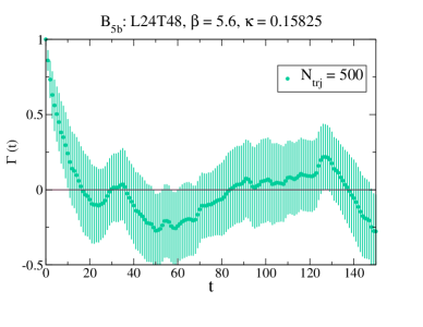
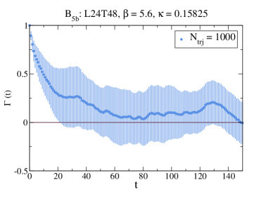
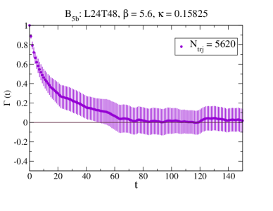
Figure 1: Autocorrelation functions for the unsmeared plaquette for the total accumulated statistics 500, 1000 and 5620 respectively at $\beta=5.6$ for the ensemble $B_{5b}$.

4 Auto-correlation Measurements

We have generated ensembles of gauge configurations by means of DD-HMC ddhmc algorithm using unimproved Wilson fermion and gauge actions wilson1 ; wilson2 with $n_{f}=2$ mass degenerate quark flavors. At $\beta=5.6$ the lattice volumes are $24^{3}\times 48$ and $32^{3}\times 64$ and the renormalized physical quark mass (calculated using axial Ward identity) ranges between $25$ to $125$ MeV ($\overline{\rm MS}$ scheme at $2$ GeV). At $\beta=5.8$ the lattice volume is $32^{3}\times 64$ and the renormalized physical quark mass ranges from $15$ to $75$ MeV. To determine the lattice spacing we plot the ratio of lattice pion mass to lattice nucleon mass versus lattice pion mass. Extrapolation of the ratio to the physical point gives the lattice spacing $a$. The lattice spacings at $\beta=5.6$ and $5.8$ are $0.069$ and $0.053$ fm respectively. The Sommer method of determining the scale agree with the quoted value of lattice spacings at $\beta=5.6$ and $\beta=5.8$ for the value of Sommer parameter $r_{0}=0.44$ fm.

The number of thermalized configurations ranges from $7000$ to $14000$. The lattice parameters and simulation statistics are given in Table 1. For all ensembles of configurations the average Metropolis acceptance rates range between $75-98\%$.

5 Results

In Fig. 1 we show the autocorrelation function for the unsmeared plaquette for the total accumulated statistics 500, 1000 and 5620 respectively for $\beta$=5.6, $\kappa=0.15825$ and lattice volume $24^{3}\times 48$. We notice that for smaller statistics, the autocorrelation function touches zero earlier leading to the underestimation of $\tau_{int}$. Also the positivity of the autocorrelation function is violated in contrast to theoretical expectations but the situation improves as statistics increases.

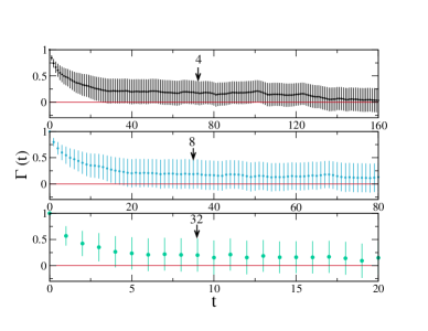
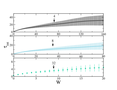
Figure 2: Normalized autocorrelation functions (left) and integrated autocorrelation times (right) for unsmeared plaquette with three different gaps ($4,8,32$) between measurements for the ensemble $C_{5}$ at $\beta=5.6$.

Since it is exorbitant to measure smeared Wilson loops, propagators and smeared topological charge on each and every trajectory, we have measured these observables for the configurations saved with specific gaps. However unsmeared plaquette ($P_{0}$) is measured on each trajectory. It is mandatory, however, to check that the measured autocorrelation scales appropriately with the gaps, so as to ensure the correct determination of the autocorrelation. We have carried out such checks and a typical result is presented in Figs. 2. In Fig. 2 we present the normalized autocorrelation functions (left) and integrated autocorrelation times (right) for unsmeared plaquette with three different gaps ($4,8,32$) between measurements for the ensemble $C_{5}$. The data clearly exhibit the scaling properties with the gaps.

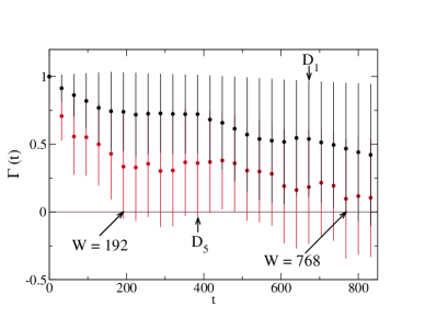
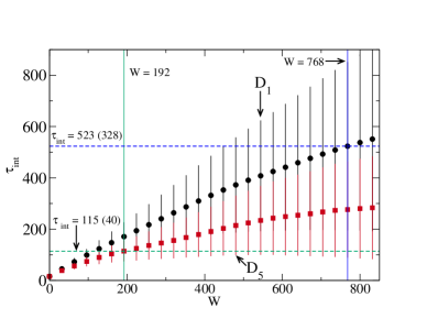
Figure 3: Normalized autocorrelation functions (left) and integrated autocorrelation times (right) for $Q_{20}^{2}$ at $\beta=5.8$ for the ensembles $D_{1}$ and $D_{5}$.

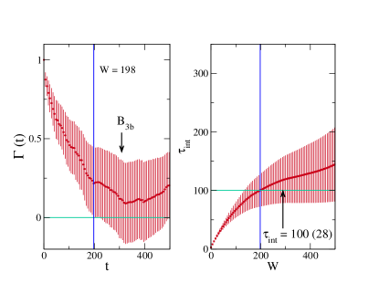
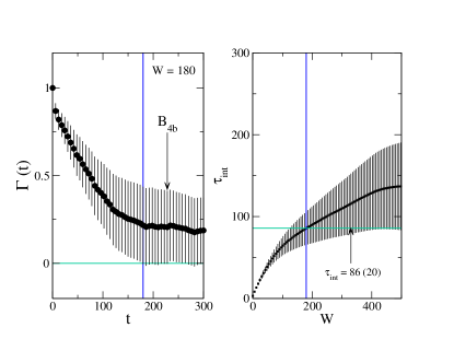
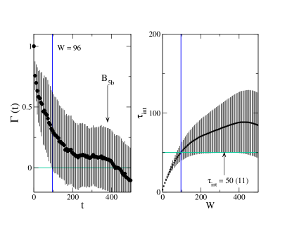
Figure 4: Normalized autocorrelation functions and integrated autocorrelation times for $Q_{20}^{2}$ at $\beta=5.6$ for the ensembles $B_{3b}$ (left), $B_{4b}$ (right) and $B_{5b}$ (bottom).

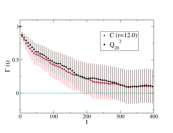
Figure 5: Normalized autocorrelation functions for $C(r=12)$ and $Q_{20}^{2}$ at $\beta=5.6$ for the ensemble $B_{3b}$.

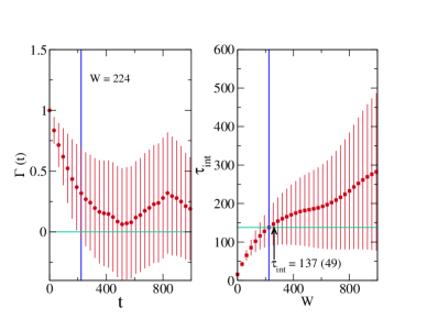
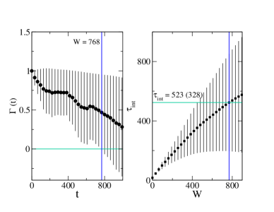
Figure 6: Normalized autocorrelation functions and integrated autocorrelation times for $C(r=12)$ (left) and $Q_{20}^{2}$ (right) at $\beta=5.8$ for the ensemble $D_{1}$.

In Figs. 3 and 4 we show noramlized autocorrelation functions and integrated autocorrelation times for $Q_{20}^{2}$ at different $\kappa$’s for $\beta=5.8$ and $\beta=5.6$ respectively. Windows are chosen as indicated by the vertical lines. Figs. 3 and 4 show that at both the lattice spacings ($\beta=5.6,5.8$) autocorrelations of $Q_{20}^{2}$ decrease with decreasing quark mass even though for the smaller quark mass at $\beta=5.8$ ($D_{5}$) molecular dynamics trajectory length ($\tau$) is smaller. Note that the trend is more visible at smaller lattice spacing ($\beta=5.8$). A possible explanation for this suppression of autocorrelation with decreasing quark mass is that the algorithm needs to span between lesser number of topological sectors at smaller quark mass since the width of the Gaussian distribution of topological charge decreases with decreasing quark mass.

In Fig. 5 we show normalized autocorrelation functions for $C(r=12)$ and $Q_{20}^{2}$ at $\beta=5.6$ for the ensemble $B_{3b}$. Fig. 5 shows that at $\beta=5.6$ the autocorrelations for $Q_{20}^{2}$ and $C(r=12)$ are very close. In Fig. 6 we show normalized autocorrelation functions and integrated autocorrelation times for $C(r=12)$ (left) and $Q_{20}^{2}$ (right) at $\beta=5.8$ for the ensemble $D_{1}$ where pion mass is comparable with the pion mass for the ensemble $B_{3b}$. Fig. 6 shows that at $\beta=5.8$ the autocorrelation for $Q_{20}^{2}$ is larger than the autocorrelation for $C(r=12)$. Figs. 5 and 6 show that autocorrelation for $Q_{20}^{2}$ increases quite significantly with decreasing lattice spacing at comparable pion mass whereas the autocorrelation of topological charge density correlator ($C(r)$) increases slightly with decreasing lattice spacing. Taking into account the effect of active link ratio (see for example section 3.1 in Ref. sommer ) ($R=0.363$ for $\beta=5.6$ and $R=0.422$ for $\beta=5.8$) strengthens this conclusion.

In Fig. 7 we present normalized autocorrelation functions (left) and integrated autocorrelation times (right) for $P_{0}$ for $\beta=5.6$ at lattice volume $24^{3}\times 48$. We find that $\tau_{int}$ for $P_{0}$ is not increasing with decreasing quark mass. In Fig. 8 we present normalized autocorrelation functions (left) and integrated autocorrelation times (right) for $W_{20}(4,4)$ for $\beta=5.6$ at lattice volume $24^{3}\times 48$. The figure shows $\tau_{int}$ for $W_{20}(4,4)$ is also not increasing with decreasing quark mass.

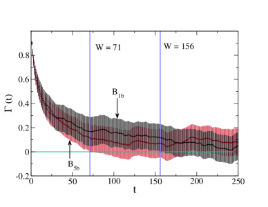
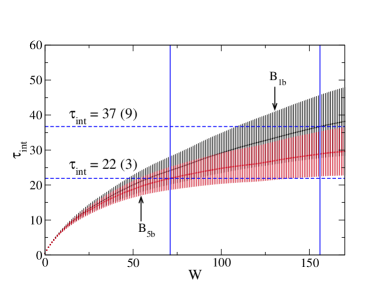
Figure 7: Normalized autocorrelation functions (left) and integrated autocorrelation times (right) for $P_{0}$ at $\beta=5.6$ for the ensembles $B_{1b}$ and $B_{5b}$.

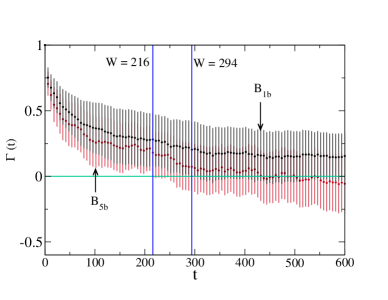
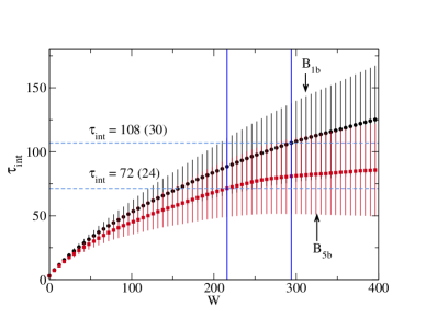
Figure 8: Normalized autocorrelation functions (left) and integrated autocorrelation times (right) for $W_{20}(4,4)$ at $\beta=5.6$ for the ensembles $B_{1b}$ and $B_{5b}$.

For the measurement of static potential $V(r)$ one needs to measure Wilson loops of various sizes. In the measurement of a Wilson loop, to suppress unwanted fluctuations smearing is needed. Therefore it is interesting to study how autocorrelation of Wilson loops changes with sizes of the Wilson loops and smearing levels. In Fig. 9 we present normalized autocorrelation functions and integrated autocorrelation times for $W_{20}$ with different sizes for the ensemble $D_{1}$. In Fig. 10 we show normalized autocorrelation functions and integrated autocorrelation times for $W(3,3)$ with different levels of HYP smearing for the ensemble $C_{2}$. We observe that the integrated autocorrelation time increases with the increasing size of the Wilson loop and also with the increasing smearing level. In the context of Wilson loop and Polyakov loop, SESAM collaboration has observed that geometrically extended observables suffer more from autocorrelation sesam with HMC algorithm.

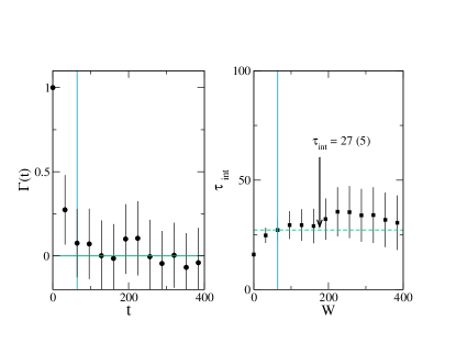
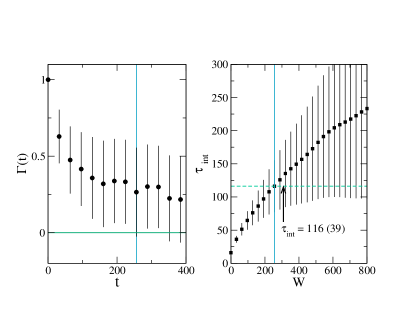
Figure 9: Normalized autocorrelation functions and integrated autocorrelation times for Wilson loops with $R=1$, $T=1$ (left) and $R=4$, $T=5$ (right) at $\beta=5.8$ for the ensemble $D_{1}$.

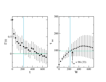
Figure 10: Normalized autocorrelation functions and integrated autocorrelation times for Wilson loops with smearing levels $=5$ (left) and smearing levels $=40$ (right) at $\beta=5.6$ for the ensemble $C_{2}$.

For hadronic observables the autocorrelations are quite small and since the number of measurements are not large the errors calculated from Eqs. (7) and (8) are quite large and mask the trends of the central values of autocorrelations. Our emphasis is on different trends of autocorrelations. To detect some trend of the central values of the autocorrelations for the hadronic observables we use a rough estimate of errors by single omission jackknife technique. In Fig. 11 integrated autocorrelation times for $PP$ propagator with wall source for three different gaps ($24,48,72$) between measurements for the ensembles $B_{4a}$ are presented. The data clearly exhibit the scaling properties with the gaps. In Table 2 integrated autocorrelation times for pion ($PP$) and nucleon propagators with wall sources at a given time slice are presented. Clearly the integrated autocorrelation time decreases with increasing $\kappa$ (i.e. decreasing quark mass) both for pion and nucleon propagators. Similar observation was made by ALPHA collaboration in the case of Clover fermion marinkovic . The autocorrelation times of pion and nucleon propagators with point source and sink (not presented here) are smaller than the gap with which configurations are saved.

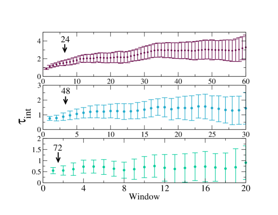
Figure 11: Integrated autocorrelation times for $PP$ propagator with wall source for three different gaps ($24,48,72$) between measurements for the ensemble $B_{4a}$ at $\beta=5.6$.

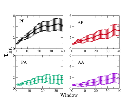
Figure 12: Integrated autocorrelation times for $PP$, $AP$, $PA$ and $AA$ correctors with wall source for the ensemble $B_{3a}$ at $\beta=5.6$. Measurements are done with a gap of 24 trajectories.

$\beta=5.6$
$tag$	$\tau_{int}^{Pion}$	$\tau_{int}^{Nucleon}$
$B_{3a}$	$99(19)$	$75(18)$
$B_{4a}$	$50(9)$	$34(9)$
$B_{5a}$	$40(10)$	$25(9)$
$C_{2}$	$39(13)$	$33(17)$
$C_{3}$	$31(15)$	$26(7)$
$C_{4}$	$34(11)$	$18(6)$

Table 2: Integrated autocorrelation times for pion ($PP$) and nucleon propagators with wall sources at $\beta=5.6$.

For the determination of pion decay constants and PCAC quark mass, pion propagators other than $PP$ are also needed. In Fig. 12 the integrated autocorrelation times for $PP$, $AP$, $PA$ and $AA$ correlators with wall source for the ensemble $B_{3a}$ are presented. The propagators with $A$ in the source are less correlated than $P$ in the source.

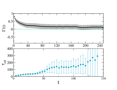
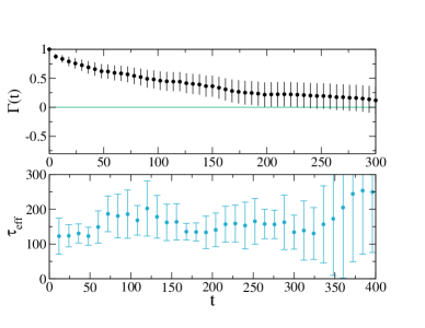
Figure 13: Normalized autocorrelation function and effective autocorrelation time for $P_{0}$ (left) $Q^{2}_{20}$ (right) for the ensemble $B_{3b}$ at $\beta=5.6$.

6 Improved estimation of $\tau_{int}$

We have seen that the autocorrelations of different observables behave differently with the change in lattice spacing. As pointed out in sommer , this behaviour is controlled by the coupling of different observables with the slow modes of the transition matrix associated with Monte Carlo Markov chain. In this reference authors have proposed a method to quantify this coupling and estimate $\tau_{int}$ more reliably. Following Ref. sommer , an improved estimation of $\tau_{\rm int}$ can be determined as follows. Let $\tau^{*}$ be the best estimate of the dominant time constant. If for an observable ${\cal O}$ all relevant time scales are smaller or of the same order of $\tau^{*}$ then the upper bound of $\tau_{\rm int}$

$$\tau^{u}_{\rm int}~{}=~{}\frac{1}{2}~{}+\Sigma_{t=1}^{W_{u}}\Gamma^{\cal O}(t)+A_{\cal O}(W_{u})~{}\tau^{*}$$ (10)

where $A_{\cal O}={\rm max}(\Gamma^{\cal O}(W_{u}),2\delta\Gamma^{\cal O}(W_{u}))$. $W_{u}$ is chosen where the autocorrelation is still significant. One possible estimation of $\tau^{*}$ is by measuring effective autocorrelation time, which is introduced in Ref. sommer as described below. Define effective exponential autocorrelation time

$$\tau_{eff}^{exp}({\cal O})=\frac{t}{2\ln{\frac{\Gamma^{\cal O}(t/2)}{\Gamma^{\cal O}(t)}}}.$$ (11)

$\tau_{eff}^{exp}$ which can be an estimate of $\tau^{*}$ is defined as,

$$\tau_{eff}^{exp}=Max_{\mathcal{O}}\left[\frac{t}{2\ln{\frac{\Gamma^{\cal O}(t/2)}{\Gamma^{\cal O}(t)}}}\right].$$ (12)

The estimation of $\tau_{eff}^{exp}({\cal O})$ requires good signal to noise ratio in the asymptotic region in a case by case basis which in turn requires very long Markov chain and is beyond the scope of the present work.

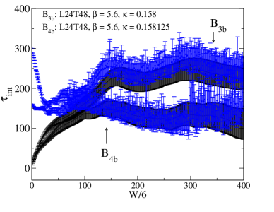
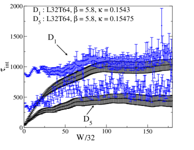
Figure 14: Integrated autocorrelation times and their upper bounds ($\tau^{u}_{int}$) for topological susceptibilities ($Q^{2}_{20}$) at $\beta$ = 5.6 (left) and at $\beta$ = 5.8 (right).

However it is interesting to look at $\tau_{eff}^{exp}({\cal O})$ where reliable data is available and we present such an example in Fig. 13 (the jackknife technique is used to calculate the error of $\tau_{eff}^{exp}({\cal O})$). In Fig. 13 it appears that $Q_{20}^{2}$ is coupling dominantly with slow mode, whereas $P_{0}$ is coupling with more than one modes; nevertheless the slowest mode appearing in $P_{0}$ is approximately the same as in $Q_{20}^{2}$. This is reflected in the behaviour of $\tau_{eff}^{exp}({\cal O})$, which shows a single plateau for $Q_{20}^{2}$, but for $P_{0}$, there is more than one plateau and the data is more noisy. Similar behaviour is observed in pure gauge theory in Ref. sommer .

In improved estimation given in Eq. (10) central value of $\tau_{int}$ gets modified. To check if this modification preserves the trend of autocorrelation of $Q_{20}^{2}$ with respect to quark mass, in Fig. 14 we present the integrated autocorrelation times and their upper bounds ($\tau^{u}_{int}$) with rough errors estimated by jackknife method for topological susceptibilities ($Q^{2}_{20}$) at $\beta$ = 5.6 (left) and at $\beta$ = 5.8 (right). At both lattice spacings, we find that both $\tau_{int}(Q^{2}_{20})$ and $\tau^{u}_{int}(Q^{2}_{20})$ decrease as quark mass decreases.

In conclusion, an extensive study of autocorrelation of several observables in lattice QCD with two degenerate flavours of naive Wilson fermion has shown that (1) at a given lattice spacing, autocorrelations of topological susceptibility and pion and nucleon propagators with wall source decrease with decreasing quark mass and autocorrelations of plaquette and Wilson loop do not increase with decreasing quark mass, (2) autocorrelation of topological susceptibility substantially increases with decreasing lattice spacing but autocorrelation of topological charge density correlator shows only mild increase and (3) increasing the size and the smearing level increase the autocorrelation of Wilson loop.

Acknowledgements

We thank Stefan Schaefer for a critical reading of an earlier version of the manuscript and for suggestions for improvement of the manuscript. Numerical calculations are carried out on Cray XD1 and Cray XT5 systems supported by the 10th and 11th Five Year Plan Projects of the Theory Division, SINP under the DAE, Govt. of India. We thank Richard Chang for the prompt maintenance of the systems and the help in data management. This work was in part based on the public lattice gauge theory codes of the MILC collaboration milc and Martin Lüscher ddhmc .

References

- (1) S. Duane, A. D. Kennedy, B. J. Pendleton, D. Roweth, Phys. Lett. B195, 216 (1987).
-
(2)
M. Lüscher, Comput. Phys. Commun. 156, 209-220 (2004).
[hep-lat/0310048]; M. Lüscher,
Comput. Phys. Commun. 165, 199-220 (2005).
[hep-lat/0409106].
http://luscher.web.cern.ch/luscher/DD-HMC/index.html - (3) S. Schaefer et al. [ALPHA Collaboration], Nucl. Phys. B 845, 93 (2011) [arXiv:1009.5228 [hep-lat]].
- (4) M. Luscher, PoS LATTICE 2010, 015 (2010) [arXiv:1009.5877 [hep-lat]].
- (5) K. G. Wilson, Phys. Rev. D10, 2445-2459 (1974).
- (6) K. G. Wilson, Quarks and Strings on a Lattice”, in New Phenomena in Subnuclear Physics, Proceedings of the International School of Subnuclear Physics, Erice, 1975, edited by A. Zichichi (Plenum, New York, 1977).
- (7) See for example, S. Basak and A. K. De, Phys. Lett. B 430, 320 (1998) [hep-lat/9801001].
- (8) N. Madras and A. D. Sokal, J. Stat. Phys. 50, 109 (1988); A. D. Sokal, Monte Carlo Mehtods in Statistical Mechanics: Foundations and New Algorithms, NATO Adv. Sci. Inst. Ser. B Phys., Vol. 361, Plenum, New York, (1997), pp. 131-192.
- (9) T. W. Anderson, The Statistical Analysis of Time Series (Wiley-Interscience, 1994).
- (10) M. B. Priestley, Spectral Analysis and Time Series (Academic Press, 1983).
- (11) U. Wolff [ALPHA Collaboration], Comput. Phys. Commun. 156, 143 (2004) [Erratum-ibid. 176, 383 (2007)] [hep-lat/0306017].
- (12) T. A. DeGrand, A. Hasenfratz, T. G. Kovacs, Nucl. Phys. B505, 417-441 (1997). [arXiv:hep-lat/9705009 [hep-lat]].
- (13) A. Hasenfratz, C. Nieter, Phys. Lett. B439, 366-372 (1998). [hep-lat/9806026].
- (14) http://physics.indiana.edu/~sg/milc.html
- (15) A. Hasenfratz, F. Knechtli, Phys. Rev. D64, 034504 (2001). [hep-lat/0103029].
- (16) A. Chowdhury, A. K. De, S. De Sarkar, A. Harindranath, S. Mondal, A. Sarkar and J. Maiti, Phys. Lett. B 707, 228 (2012) [arXiv:1110.6013 [hep-lat]].
- (17) A. Chowdhury, A. K. De, S. De Sarkar, A. Harindranath, S. Mondal, A. Sarkar and J. Maiti, PoS LATTICE 2011, 099 (2011) [arXiv:1111.1812 [hep-lat]].
- (18) A. Chowdhury, A. K. De, A. Harindranath, J. Maiti and S. Mondal, “Topological charge density correlator in Lattice QCD with two flavours of unimproved Wilson fermions”, arXiv:1208.4235v1 [hep-lat].
- (19) Th. Lippert, G. Bali, N. Eicker, L. Giusti, U. Glassner, S. Gusken, H. Hoeber, P. Lacock, G. Martinelli, F. Rapuano, G. Ritzenhofer, K. Schilling, G. Siegert, A. Spitz, P. Ueberholz, and J. Viehoff, Nucl. Phys. Proc. Suppl. 60A, 311 (1998) [hep-lat/9707004].
- (20) M. Marinkovic, S. Schaefer, R. Sommer and F. Virotta, arXiv:1112.4163 [hep-lat].