The Andreev states of a superconducting quantum dot: mean field vs exact numerical results

Abstract

We analyze the spectral density of a single level quantum dot coupled to superconducting leads focusing on the Andreev states appearing within the superconducting gap. We use two complementary approaches: the numerical renormalization group and the Hartree-Fock approximation. Our results show the existence of up to four bound states within the gap when the ground state is a spin doublet ($\pi$ phase). Furthermore the results demonstrate the reliability of the mean field description within this phase. This is understood from a complete correspondence that can be established between the exact and the mean field quasiparticle excitation spectrum within the gap.

I Introduction

Much progress has been achieved in recent years on the transport properties of quantum dots coupled to superconducting leads (for a review see us2011 ). A central concept in the understanding of these properties is that of Andreev bound states (ABS), i.e. the bound states appearing within the superconducting gap due to multiple Andreev reflections at the dot superconductor interfaces. When the two leads are superconducting the ABS depend on the superconducting phase difference and are thus current carrying states (typically most of the Josephson current is carried by the ABS us2011 ). The interest in the ABS in these kind of systems has been increased by recent experiments allowing for their direct measurement through tunnel spectroscopy on carbon nanotube and graphene quantum dots pillet2010 ; dirks . The issue is also related to the strong activity in the search of Majorana fermions, which would manifest as midgap states in different type of hybrid nanostructures alicea .

The simplest situation for analyzing the ABS spectrum is that of a single quantum dot (QD) with large energy level spacing which can be appropriately described by the single level Anderson model anderson61 . The presence of subgap states for the case of a magnetic impurity in a BCS superconducting host was already demonstrated in Refs. shiba ; jarrel . This model was afterward extended to analyze the Josephson transport properties and the so called 0-$\pi$ transition which signals the transition from a singlet ($S=0$) to a doublet ($S=1/2$) ground state glazman ; arovas ; vecino ; choi2 ; siano ; oguri ; ansari . In spite of these theoretical efforts the knowledge about the detailed structure of the ABS spectrum appears to be somewhat disperse in the literature. Thus, in a method like the non-crossing approximation (NCA), which is able to describe the 0-$\pi$ transition in the large charging energy regime, a single subgap resonance appears whose crossing of the Fermi level signals the transition sellier . On the other hand, other approximations like Hartree-Fock (HFA) or exact diagonalizations in the infinite $\Delta$ limit, where $\Delta$ denotes the superconducting gap parameter in the leads, point to the existence of up to 4 levels symmetrically located around the Fermi energy in the $\pi$-phase vecino ; simon ; luitz . The bound state spectrum has also been analyzed using the numerical renormalization group (NRG) method choi ; hewson ; hecht although in these works only up to two ABS were identified. A previous NRG calculation showing up to four ABS exists japs although in this work only the single lead case was considered (i.e. without a phase difference between the leads). Taking into account all this rather fragmented evidence it seems worthwhile to investigate this issue in more detail using numerically exact results compared to different approximations. This is further motivated by the possibility of a direct experimental test along the lines of recent works pillet2010 ; dirks .

In the present work we give a detailed analysis of the ABS for the single level Anderson model coupled to superconducting leads focusing in the regime $T_{K}<\Delta$, where $T_{K}$ denotes the Kondo temperature, which appears to be the relevant one for describing the experimental results of Ref. pillet2010 . We use NRG calculations and compare the results with the mean-field approach provided by the HFA. It is found that when the system undergoes the transition to the $\pi$-phase there appear in general up to 4 ABS in agreement with the analysis of the simple spin-polarized HFA vecino . Indeed, our analysis shows that the HFA provides a quite fair description of the bound state spectra except in the regime where Kondo correlations dominate over the superconducting ones.

The rest of the paper is organized as follows: in Sect. II we describe the model used for a QD coupled to superconducting leads and the basic theoretical analysis of its spectral properties; in Sect. III we consider the simpler situation of a QD coupled to a single superconducting electrode (S-QD case) and present results for the ABS spectrum using both NRG and HFA, analyzing the range of validity of this last approximation for this case. In Sect. IV this analysis is extended to a phase-biased S-QD-S system where we study in particular the behavior of the ABS spectrum around the transition between singlet and doublet ground states. Finally in Sect. V we give some concluding remarks.

II Model and basic theoretical analysis

A minimal model for a QD coupled to metallic electrodes in the regime where the energy level spacing $\delta\epsilon$ is sufficiently large to restrict the analysis to a single spin-degenerate level is provided by the single level Anderson model anderson61 , with the Hamiltonian $H=H_{L}+H_{R}+H_{T}+H_{QD}$ where $H_{QD}$ corresponds to the uncoupled dot given by

$$H_{QD}=\sum_{\sigma}\epsilon_{0}c^{\dagger}_{0\sigma}c_{0\sigma}+Un_{0\uparrow}n_{0\downarrow},$$ (1)

where $c^{\dagger}_{0\sigma}$ creates and electron with spin $\sigma$ on the dot level located at $\epsilon_{0}$ and $U$ is the local Coulomb interaction for two electrons with opposite spin within the dot ($n_{0\sigma}=c^{\dagger}_{0\sigma}c_{0\sigma}$). On the other hand, $H_{L,R}$ describe the uncoupled left and right leads which are superconductors represented by a BCS Hamiltonian of the type

$$H_{\nu}=\sum_{k\sigma}\xi_{k,\nu}c^{\dagger}_{k\sigma,\nu}c_{k\sigma,\nu}+\sum_{k}\left(\Delta_{\nu}c^{\dagger}_{k\uparrow,\nu}c^{\dagger}_{-k\downarrow,\nu}+\mbox{h.c.}\right),$$ (2)

where $c^{\dagger}_{k\sigma,\nu}$ creates an electron with spin $\sigma$ at the single-particle energy level $\xi_{k,\nu}$ of the lead $\nu=L,R$ (usually referred to the lead chemical potential, i.e. $\xi_{k,\nu}=\epsilon_{k,\nu}-\mu_{\nu}$) and $\Delta_{\nu}=|\Delta_{\nu}|\exp{(i\phi_{\nu})}$ is the (complex) superconducting order parameter on lead $\nu$. Finally, $H_{T}$ describes the coupling between the QD level to the leads and has the form

$$H_{T}=\sum_{k\sigma,\nu}\left(V_{k,\nu}c^{\dagger}_{k\sigma,\nu}c_{0\sigma}+\mbox{h.c.}\right).$$ (3)

The coupling to the leads is usually characterized by a single parameter $\Gamma_{\nu}=\pi\rho_{\nu}|V_{\nu}|^{2}$, determining the width of the one-electron resonance. In this expression $V_{\nu}$ corresponds to an average over the Fermi surface of $V_{k,\nu}$ and $\rho_{\nu}$ denotes the corresponding density of states on the leads.

In this work we are interested in the spectral properties which can be extracted from the dot Green’s functions defined as $\hat{G}^{r}_{\sigma}(t,t^{\prime})=-i\theta(t-t^{\prime})\langle\left[\Psi_{\sigma}(t),\Psi^{\dagger}_{\sigma}(t^{\prime})\right]_{+}\rangle$, where $\Psi_{\sigma}=(c_{0\sigma}\;c^{\dagger}_{0,-\sigma})^{T}$ and the average is taken over the system ground state. In the case of the Anderson model with superconducting leads two types of ground states appear depending on the parameters: a non-degenerate $S=0$ ground state (0 phase) or a double-degenerate $S=1/2$ ground state ($\pi$-phase). The Green’s functions can be formally written in frequency space using the Lehmann representation

$$\hat{G}^{r}_{\sigma,S_{z}}(\omega)=\sum_{m}\frac{\langle\Phi_{0,S_{z}}|\Psi_{\sigma}|\Phi_{m}\rangle\langle\Phi_{m}|\Psi^{\dagger}_{\sigma}|\Phi_{0,S_{z}}\rangle}{\omega-\left(E_{m}-E_{0}\right)+i0^{+}}+\frac{\langle\Phi_{0,S_{z}}|\Psi^{\dagger,T}_{\sigma}|\Phi_{m}\rangle\langle\Phi_{m}|\Psi_{\sigma}^{T}|\Phi_{0,S_{z}}\rangle}{\omega+\left(E_{m}-E_{0}\right)+i0^{+}},$$ (4)

where the system ground state, denoted by $|\Phi_{0,S_{z}}\rangle$, maybe degenerate ($S_{z}=\pm 1/2$) and $m$ labels the excited states having an extra quasiparticle with respect to the ground state. In the degenerate case the total Green function is finally obtained as $\hat{G}^{r}_{\sigma}=\frac{1}{2}\sum_{S_{z}}\hat{G}^{r}_{\sigma,S_{z}}.$ The formal expression of Eq. (4) allows a direct calculation of the quasiparticle spectral densities using numerical methods like the NRG method which we describe further below.

It would be interesting to compare the NRG results for the spectral density with those provided by different approximations specially with HFA which could provide a rather simple scheme for describing recent experimental results on the ABS spectrum pillet2010 . In this approximation the dot Green’s function is given by $(\hat{G}^{r,HF}_{\sigma})^{-1}=(\hat{G}^{r,(0)})^{-1}-\hat{\Sigma}^{HF}_{\sigma}$, where $\hat{G}^{r,(0)}$ is the non-interacting dot Green’s function in Nambu space and the self-energy $\hat{\Sigma}^{HF}_{\sigma}$ corresponds to the first order diagrams in the Coulomb interaction and are given by

$$\Sigma^{HF}_{11,\sigma} = -\Sigma^{HF}_{22,-\sigma}=U<n_{0,-\sigma}>$$

$$\Sigma^{HF}_{12,\sigma} = (\Sigma^{HF}_{21,\sigma})^{*}=-U<c_{0\uparrow}c_{0\downarrow}>$$ (5)

In the HFA both $<n_{0,\sigma}>$ and $<c_{0\uparrow}c_{0\downarrow}>$ have to be calculated self-consistently. The explicit expression for $\hat{G}^{r,HF}$ is

$$\hat{G}^{r,HF}_{\sigma}=\left(\begin{array}[]{cc}\omega-\epsilon_{0}-\Gamma g(\omega)-\Sigma^{HF}_{11,\sigma}&\Gamma\cos{\frac{\phi}{2}}f(\omega)-\Sigma^{HF}_{12,\sigma}\\ \Gamma\cos{\frac{\phi}{2}}f(\omega)-\Sigma^{HF}_{21,\sigma}&\omega+\epsilon_{0}-\Gamma g(\omega)-\Sigma^{HF}_{22,\sigma}\end{array}\right)^{-1}$$ (6)

where $\Gamma_{L}=\Gamma_{R}=\Gamma/2$, $\phi$ denotes the superconducting-phase difference and $g(\omega)=-\Delta f(\omega)/\omega=-\omega/\sqrt{\Delta^{2}-\omega^{2}}$ are the dimensionless BCS Green’s functions of the uncoupled leads.

Within the HFA the transition from the 0 to the $\pi$ phase shiba ; arovas ; vecino is signaled by the existence of a spin broken symmetry solution with $<n_{0,\sigma}>\neq<n_{0,-\sigma}>$. Although this symmetry breaking is not actually present in the exact solution, the HFA provides a very accurate description of the ABS spectrum within the $\pi$ phase as will be shown along this work. This can be qualitatively understood by analyzing the low energy pole structure of the exact Green’s function given by Eq. (4) when the system is in the $\pi$-phase. In this case the two-fold degenerate ground state can be labeled by $S_{z}=\pm 1/2$. Quasiparticle excitations over this ground state can correspond to transitions to states with total spin either $S=0$ or $S=1$. However, in the last case the excitation energy is necessarily larger than $\Delta$ as these excited states involve an unpaired electron in the leads. Therefore the excitations within the gap can only arise from transitions to states with total spin equal to zero. It is then straightforward to see that subgap electron-like excitations with spin $\sigma$ can only be created from the ground state with $S_{z}=-\sigma$ while the hole-like excitations arise from the ground state $S_{z}=\sigma$. This structure is illustrated in Fig. 1 where we show schematically the subgap poles in $G_{\sigma,S_{z}}(\omega)$ in the $\pi$-phase for $S_{z}=\pm 1/2$. This is precisely the structure of the subgap excitations which are found in the spin-polarized HFA: the solutions for the majority and minority spin populations have only hole-like or electron-like character respectively. Therefore one can establish a correspondence between the exact and the HFA excitations for the subgap states in the $\pi$ phase. This correspondence based on the separation of electron and hole-like excitations is specially clear in the large $\Delta$ limit which we discuss in what follows.

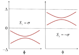
Figure 1: (Color online) Subgap pole structure of the Green’s functions components $G_{\sigma,S_{z}}(\omega)$ in the $\pi$-phase for the two different orientations of the ground state spin $S_{z}$. As discussed in the text these excitations have either a purely hole-like or electron-like character, which allows a correspondence with the results of the HFA. Spin-symmetry is recovered when taking the trace over the degenerate ground state.

$\Delta\rightarrow\infty$ case: As shown in previous works vecino ; hewson ; simon the problem can be exactly diagonalized in this limit which already illustrates in a simple way the 0-$\pi$ transition. The states can be classified according to the total spin $S=0$ or $S=1/2$. In the $S=1/2$ sector the energy levels are simply $\epsilon_{0}$ (doubly degenerate) while in the $S=0$ case the states are given by $E_{0,\pm}=\epsilon_{0}+U/2\pm\sqrt{(\epsilon_{0}+U/2)^{2}+\Gamma^{2}\cos^{2}{\phi/2}}$, leading to a phase transition for $\epsilon_{0}>E_{0,-}$. Thus, in the $\pi$-phase the spectral density contains four ABS located at $\pm U/2\pm\sqrt{(\epsilon_{0}+U/2)^{2}+\Gamma^{2}\cos^{2}{\phi/2}}$.

It is quite straightforward to see that this spectrum is recovered exactly by the HFA. Indeed, in this limit the self-consistent HF solution is

$$\hat{G}^{r,HF}_{\sigma}(\omega)\rightarrow\hskip 170.71652pt$$

$$\left(\begin{array}[]{cc}\omega-\epsilon_{0}+(2\sigma-1)\frac{U}{2}&\Gamma\cos{\frac{\phi}{2}}\\ \Gamma\cos{\frac{\phi}{2}}&\omega+\epsilon_{0}+(2\sigma+1)\frac{U}{2}\end{array}\right)^{-1}$$ (9)

which exhibits the same spectrum as the exact solution. As in the $\pi$-phase $U/2>\sqrt{(\epsilon_{0}+U/2)^{2}+\Gamma^{2}\cos^{2}{\phi/2}}$ the excitations for $\sigma=1/2$ have a hole-like character while those for $\sigma=-1/2$ have an electron character. Therefore, it is not surprising that this approximation provides a rather good description of the ABS spectrum in the $\pi$-phase for the full model.

III ABS spectrum for the S-QD case

Before discussing the general case with two S leads and fixed phase difference it is worth analyzing the simpler case of an Anderson impurity coupled to a single BCS lead. This model exhibits also a transition to a degenerate $S=1/2$ ground state and its spectral properties are relevant to understand the transport properties in N-QD-S systems when $\Gamma_{N}\ll\Delta$ deacon . To obtain the numerically exact ABS spectrum for this case we have implemented an NRG algorithm following the lines of Refs. japs ; choi2 ; karrasch . The idea behind the method is to discretize the energy levels in the leads on a logarithmic grid of energies $\Lambda^{-n}$ (with the dimensionless parameter $\Lambda>1$ and $1\leq n\leq N\rightarrow\infty$) with exponentially high resolution on the low-energy excitations. This discretization allows then to map the impurity model into a linear “tight-binding” chain with hopping matrix elements decaying as $\Lambda^{-n/2}$ with increasing site index $n$. The sequence of Hamiltonians which is constructed by adding a new site in the chain is then diagonalized iteratively. As the number of states grows exponentially an adequate truncation scheme is required.

The cutoff parameter $\Lambda$ (as defined originally in Ref. krishna ) is chosen in order to ensure convergence of the spectral properties inside the gap. Depending on the value of $U/\Gamma$ and the ratio $T_{K}/\Delta$, we have chosen $\Lambda$ varying between 2 and 4. For most of the results shown below we have checked that the value $\Lambda=4$ provides already well converged results. In all the cases the usual correction $\Gamma_{NRG}=A_{\Lambda}\Gamma$, where

$$A_{\Lambda}=\frac{1}{2}\frac{1+1/\Lambda}{1-1/\Lambda}\ln\Lambda$$

is used in order to correctly reproduce the exact $\Lambda\rightarrow 1$ limit krishna ; japs ; karrasch . On the other hand, the maximum number of states $N_{c}$ kept in the iterative NRG procedure vary between $\sim 300$ in the S-QD case to $\sim 800$ for the S-QD-S case.

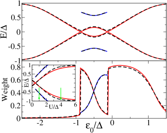
Figure 2: (Color online) Upper panel: ABS spectrum of the S-QD system for the case $U/\Delta=1$ and $\Gamma/\Delta=0.2$ as a function of the dot level position $\epsilon_{0}$, calculated using the NRG (full lines) and HFA (dashed lines) respectively. The $\pi$-phase appearing around $\epsilon_{0}/\Delta\sim-0.5$ is characterized by the crossing of the internal Andreev levels and the presence of two extra states around $E\sim\pm 0.5\Delta$, which disappear within the 0-phase. The lower panel depicts the corresponding weights in the spectral density for the electron-like quasiparticle excitations. The inset shows the behavior of the ABS as a function of $U/\Delta$ in the electron-hole symmetric case $\epsilon_{0}=-U/2$. The arrows in this plot indicate the $U/\Delta$ cases shown in the main frames of Figs. 2 and 3 respectively.

In typical experiments the charging energy $U$ adopts a nearly fixed value $U>\Gamma$ while the dot level position can be varied. We thus first analyze the evolution of the ABS spectrum as a function of $\epsilon_{0}$ for fixed $U/\Delta$ and $\Gamma/\Delta$. Fig. 2 shows the ABS spectrum and the corresponding weights for $U/\Delta=1$ and $\Gamma/\Delta=0.2$ obtained both within the NRG method and the HFA. The weights of the spectral density are calculated from the residues of the Green’s functions (Eqs. (4) and (6)) at the poles corresponding to the ABS energies.

It is first worth noticing that the spectrum is characterized by the presence of 4 ABS in the region $|\epsilon_{0}+U/2|<U/2$, which corresponds to the $S=1/2$ ground state, while only two ABS are present outside this region where the ground state is a singlet. As can be observed the HFA fairly reproduces not only the level positions but also their weights. Notice that the weights represented in the lower panels of Figs. 2, 3 correspond only to the electron like excitations which explains the asymmetry between positive and negative $\epsilon_{0}$ values.

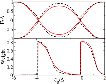
Figure 3: (Color online) Upper panel: ABS spectrum of the S-QD system for $U/\Delta=4$ and $\Gamma/\Delta=0.2$ as a function of the dot level position $\epsilon_{0}$ calculated using the NRG (full lines) and HFA (dashed lines) respectively. Notice that the outermost Andreev bound states have already merged with the continuum for this choice of parameters. The lower panel depicts the corresponding spectral weight for the electron-like excitations.

With increasing $U$ the outermost ABS within the $S=1/2$ phase gradually approach the gap edge while its weight is reduced. Eventually, these states disappear for $U/\Delta\sim 2$, as can be noticed in the inset of Fig. 2 which corresponds to the symmetric case. The ABS spectrum properties for $U/\Delta=4$, illustrated in Fig. 3, clearly exhibits only two ABS within the gap. Again, as in the $U/\Delta=1$ case the agreement between the NRG results and the HFA is quite satisfactory. The main difference between both results appears at the crossing points between the magnetic and non-magnetic regions where the HFA exhibits a small discontinuity. This discontinuity is due to the coexistence around these points of both types of solution in the HFA. In the results represented in Figs. 3 and 4 only the most stable HFA solution is shown.

As a general remark one could state that the HFA reproduces fairly well the NRG results for arbitrary dot occupancy as far as the Kondo temperature $T_{K}=\sqrt{U\Gamma/2}\exp{(-\pi U/8\Gamma)}$ of the e-h symmetric case is smaller than $\Delta$. Deviations with respect to the NRG results could be expected when $\Delta/T_{K}$ becomes sufficiently small. This is illustrated in Fig. 4 where the ABS spectrum is shown for the e-h symmetric case as a function of $\Delta/T_{K}$. As can be observed, when $\Delta/T_{K}<5$ the HFA results clearly deviates from the NRG ones as it predicts a magnetic solution up to the limit $\Delta/T_{K}\rightarrow 0$ (i.e. deep in the Kondo regime) whereas the NRG result becomes non-magnetic for $\Delta/T_{K}\sim 2.8$. In contrast, in the opposite limit $\Delta/T_{K}\gg 1$ both results converge asymptotically to the $\Delta\rightarrow\infty$ spectrum discussed in the previous section. We should point out that for the $U/\Gamma$ ratio used in Fig. 4 the “universal” limit (i.e. where all quantities depend only on the ratio $\Delta/T_{K}$) is still not reached. For larger $U/\Gamma$ ratios the transition occurs at smaller $\Delta/T_{K}$, converging to a value $\sim 1.7$ when $U/\Gamma>10$. This value is similar to the one reported in japs but somewhat larger than the one of Ref. siano obtained using quantum Monte Carlo techniques. One should notice also the difference in the definition of $T_{K}$ used in Refs. japs ; hewson , which corresponds to $0.4107$ times the one used in the present work and also in Refs. choi2 ; siano ; choi ; karrasch (the relation between the two definitions can be found in hewson-book ).

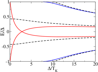
Figure 4: (Color online) ABS spectrum of the S-QD system as a function of $\Delta/T_{K}$, where $T_{K}$ is the Kondo temperature for the electron-hole symmetric case taking $U/\Gamma=5$. Red and blue (full) lines correspond to the NRG calculation while black (dashed) lines are the HFA results.

IV ABS spectrum for the S-QD-S case

We analyze in this section the behavior of the ABS spectrum as a function of the phase difference for the S-QD-S case. The results shown in Fig. 5 correspond to the case $U=\Delta$ and $\Gamma=0.2\Delta$, already analyzed in the previous section, for different values of the dot level illustrating the transition from the $\pi$ to the $0$ phase. The upper panel of Fig. 5 corresponds to the electron-hole symmetric case where the system exhibits 4 ABS inside the gap (notice that in the figure only the two electron-like states are shown). The agreement between NRG and HFA is in this regime fairly good, as was already evident in Fig. 2 (which corresponds to the $\phi=0$ in this plot). When traversing the transition (middle panel of Fig. 5) the agreement is less satisfactory due to the fact that the HFA result fully corresponds to the 0 phase whereas within NRG the system is in a mixed 0’ state (i.e. a mixed phase of $0$ character at $\phi=0$ and $\pi$ character at $\phi=\pi$ with the absolute minimum energy corresponding to $\phi=0$, see Ref. arovas ). Finally, when the level position is sufficiently low both approaches predict a 0 phase and the agreement in the ABS spectrum becomes progressively quite satisfactory again. This is the same trend which can be observed in Figs. 2 and 3.

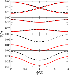
Figure 5: Evolution of the phase-dependent ABS spectrum when varying the dot level position for $U/\Delta=1$ and $\Gamma/\Delta=0.2$ calculated using the NRG method (full lines) and the HFA (dashed lines). From upper to lower panel $\epsilon_{0}/\Delta=-0.5,-0.7,-0.95,-1.2$. Notice that only the electron part of the spectrum is shown and that a different scale on the vertical axis is used for each panel in order to better visualize the details of the curves.

V Conclusions

In this work we have analyzed the subgap spectral density of a single dot coupled to superconducting leads with the aim of clarifying some of the features of the ABS which appear to be controversial in the literature. By means of numerically exact NRG calculations we have shown that in general up to 4 ABS appear when the ground state becomes magnetic, i.e. in the $\pi$-phase. Within this phase the four states eventually reduce to only two for increasing $U/\Delta$. Although the states are located symmetrically with respect to the Fermi level the electron-hole symmetry is in general broken. We have shown that this behavior is adequately reproduced by the HFA for a broad range of parameters, except very close to the transition regions between the different phases. This approximation, however, is unable to reproduce the correct behavior in the strong Kondo regime when $T_{K}\gg\Delta$.

References

References

- (1) Martín-Rodero A and Levy Yeyati A 2011 Adv. Phys. 60 899
- (2) Pillet J D Quay C H L Morfin P Bena C Levy Yeyati A Joyez P 2010 Nature Phys. 6 965
- (3) Dirks T Hughes T L Lal S Uchoa B Chen Y F Chialvo C Goldbart P M and Mason N 2011 Nature Phys. 7 386
- (4) Alicea J 2012 Rep. Prog. Phys. 75 076501
- (5) Anderson P W 1961 Phys. Rev. 124 41
- (6) Shiba H 1973 Prog. Theor. Phys. 50 50
- (7) Jarrel M Silvia D S and Patton B 1990 Phys. Rev. B 42 4804
- (8) Glazman L I and Raikh M E 1988 JETP Lett. 47 452 2788
- (9) Rozhkov A V and Arovas D P 1999 Phys. Rev. Lett. 82 2788
- (10) Vecino E Martín-Rodero A and Levy Yeyati A 2003 Phys. Rev. B 68 035105
- (11) Choi M S Lee M Kang K and Belzig W 2004 Phys. Rev. B 70 020502
- (12) Siano F and Egger R 2004 Phys. Rev. Lett. 93 047002 ; Siano F and Egger R 2005 Phys. Rev. Lett. 94 039902
- (13) Oguri A Tanaka Y and Hewson A C 2004 J. Phys. Soc. Jpn. 73 2494
- (14) Ansari M H and Wilhelm F K 2011 Phys. Rev. B 84 235102
- (15) Sellier G Kopp T Kroha J and Barash Y S 2005 Phys. Rev. B 72 174502
- (16) Meng T Florens S and Simon P 2009 Phys. Rev. B 79 224521
- (17) Luitz D J and Assaad F F 2010 Phys. Rev. B 81 024509
- (18) Lim J S and Choi M S 2008 J. Phys.: Condens. Matter 20 415225
- (19) Bauer J Oguri A and Hewson A C 2007 J. Phys.: Condens. Matter 19 486211
- (20) Hecht T Weichselbaum A von Delft J and Bulla R 2008 J. Phys.: Condens. Matter 20 275213 (2008).
- (21) Yoshioka T and Ohashi Y 2000 J. Phys. Soc. Jap. 69 1812
- (22) Deacon R S Tanaka Y Oiwa A Sakano R Yoshida K Shibata K Hirakawa K and Tarucha S 2010 Phys. Rev. Lett. 104 076805
- (23) Karrasch C Oguri A and Meden V 2008 Phys. Rev. B 77 024517
- (24) Krishna-Murthy H Wilkins J and Wilson K 1980 Phys. Rev. B 21 1003
- (25) Hewson A C 1993 The Kondo problem to heavy fermions (Cambridge University Press)