Local Multifractal Analysis

Abstract.

We introduce a local multifractal formalism adapted to functions, measures or distributions which display multifractal characteristics that can change with time, or location. We develop this formalism in a general framework and we work out several examples of measures and functions where this setting is relevant.

1. Introduction

Let $f$ denote a function, a positive Radon measure, or, more generally, a distribution defined on a nonempty open set $\Omega$. One often associates with $f$ a pointwise exponent, denoted by $h_{f}(x)$, which allows to quantify the local smoothness of $f$ at $x$. On the mathematical side, the purpose of multifractal analysis is to determine the fractal dimension of the level sets of the function $x\mapsto h_{f}(x)$. Let

$$E_{H}=\{x:\;\;h_{f}(x)=H\}.$$

The multifractal spectrum of $f$ (associated with the regularity exponent $h_{f}$) is

$$d_{f}(H)=\dim\,E_{H}$$

(where $\dim$ denotes the Hausdorff dimension, see Definition 3). Multifractal spectra yield a description of the local singularities of the function, or measure, under consideration.

Regularity exponents (and therefore the multifractal spectrum) of many functions, stochastic processes, or measures used in modeling can be theoretically determined directly from the definition. However, usually, one cannot recover these results numerically on simulations, because the exponents thus obtained turn out to be extremely erratic, everywhere discontinuous functions it is for instance the case of Lévy processes [32], or of multiplicative cascades (see the book [10], and, in particular the review paper by J. Barral, A. Fan, and J. Peyrière) so that a direct determination of $h_{f}(x)$ leads to totally instable computations. A fortiori, the estimation of the multifractal spectrum from its definition is unfeasable. The multifractal formalism is a tentative way to bypass the intermediate step of the determination of the pointwise exponent, by relating the multifractal spectrum directly with averaged quantities that are effectively computable on experimental data. Such quantities can usually be interpreted as global regularity indices. For instance, the first one historically used in the function setting ($\zeta_{f}(p)$, referred to as Kolmogorov scaling function) can be defined as follows; for the sake of simplicity, we only consider in this introduction the function setting and we assume here that the functions considered are defined on the whole $\mathbb{R}^{d}$.

Recall that the Lipschitz spaces are defined, for $s\in(0,1)$, and $p\in[1,\infty]$, by $f\in\mbox{Lip}(s,L^{p}(\mathbb{R}^{d}))$ if $f\in L^{p}$ and $\exists C>0$ such that $\forall h>0$,

$$\parallel f(x+h)-f(x)\parallel_{L^{p}}\leq Ch^{s}.$$ (1)

(the definition for larger $s$ requires the use of higher order differences, and the extension to $p<1$ requires to replace Lebesgue spaces by Hardy spaces, see [34]). Then

$$\zeta_{f}(p)=p\cdot\sup\{s:f\in\mbox{Lip}(s,L^{p}(\mathbb{R}^{d}))\}.$$ (2)

Initially introduced by U. Frisch and G. Parisi in the mid 80s, the purpose of multifractal analysis is to investigate the relationships between the pointwise regularity information supplied by $d_{f}(H)$ and the global regularity information supplied by $\zeta_{f}(p)$. Note that these quantities can be computed on the whole domain of definition $\Omega$ of $f$, or can be restricted to an open subdomain $\omega\subset\Omega$. A natural question is to understand how they depend on the region $\omega$ where they are computed. It is remarkable that, in many situations, there is no dependency at all on $\omega$; we will then say that the corresponding quantity is homogeneous. It is the case for several classes of stochastic processes. For instance, sample paths of Lévy processes (and fields) [24, 25, 32], Lévy processes in multifractal time [15], and fractional Brownian motions (FBM) almost surely have homogeneous Hölder spectra, and, in the case of FBM, the Legendre spectrum also is homogeneous, see [33, 35]. In the random setting, it is also the case for many examples of multiplicative cascades, see [12]. Many deterministic functions or measures also are homogeneous (homogeneity is usually not explicitly stated as such in the corresponding papers, but is implicit in the determination of the spectra). This is for instance the case for self-similar or self-conformal measures when one assumes the so-called open set condition, or for Gibbs measures on conformal repellers (see for instance [47, 48, 50]). It is also the case for many applications, for instance the Legendre spectra raising from natural experiments (such as turbulence, see [2, 4] and references therein) are found to be homogeneous.

On the opposite, many natural objects, either theoretical or coming from real data, have been shown to be non-homogeneous : Their multifractal characteristics depends on the domain $\Omega$ over which they are observed:

• It is the case of some classes of Markov processes, see [9] and Section 5.2, and also of some Markov cascades studied in [8].

• Some self-similar measures when the open set condition is relaxed into the weak-separation condition may satisfy the multifractal formalism only when restricted to some intervals (see [56, 30, 57, 29]).

• In applications, many types of signals, which have a human origin, can have multifractal characteristics that change with time: A typical example is supplied by finance data, see [2], where changes can be attributed to outside phenomena such as political events, but also to the increasing sophistication of financial tools, which may lead to instabilities (financial crises) and implies that some characteristic features of the data, possibly captured by multifractal analysis, evolve with time. This situation is also natural in image analysis because of the occlusion phenomenon; indeed, a natural image is a patchwork of textures with different characteristics, so that its global spectrum of singularities reflects the multifractal nature of each component, and also of the boundaries (which may also be fractal) where discontinuities appear. Note that the notion of local Hausdorff dimension which plays a central role in this section, has been introduced in [38] precisely with the motivation of image analysis.

• Functions spaces with varying smoothness have been introduced motivated by the study of the relationship between general pseudo-differential operators and later by questions arising in PDEs, see [52] for a review on the subject; scaling functions with characteristics depending on the location are then the natural tool to measure optimal regularity in this context. We will investigate this relationship in Section 7.

This paper will provide new examples of multifractal characteristics which depend on the domain of observation. In such situations, the determination of a local spectrum of singularities for each “component” $\omega\subset\Omega$ will carry more information than the knowledge of the “global” one only. A natural question is to understand how the different quantities which we have introduced depend on the region $\omega$ where they are computed.

Some of the notions studied in this paper have been already introduced in [9]; let us also mention that a local $L^{q}$-spectrum was already introduced in [39], where the authors studied this notion for measures in doubling metric spaces (as well as the notion of local homogeneity) and obtained, for instance, upper bounds for the dimensions of the sets of points with given lower and upper local dimensions using this local concepts. The goal of their approach was to investigate conical density and porosity questions. In our paper, on top of measures, we also deal with functions, get comparable upper bounds for the multifractal spectra, and the examples we develop are very different.

Let us now make precise the notion we started with, namely pointwise regularity. The two most widely used exponents are the pointwise Hölder exponent of functions and the local dimension of measures. In the following, $B(x_{0},r)$ denotes the open ball of center $x_{0}$ and radius $r$.

Definition 1.

Let $\mu$ be a positive Radon measure defined on an open subset $\Omega\subset\mathbb{R}^{d}$. Let $x_{0}\in\Omega$ and let ${\alpha}\geq 0$. The measure $\mu$ belongs to $h^{\alpha}(x_{0})$ if

$$\exists C,R>0,\;\forall r\leq R,\hskip 28.45274pt\mu(B(x_{0},r))\leq Cr^{\alpha}.$$ (3)

Let $x_{0}$ belong to the support of $\mu$. The lower local dimension of $\mu$ at $x_{0}$ is

$$h_{\mu}(x_{0})=\sup\{\alpha:\mu\in h^{\alpha}(x_{0})\}=\liminf_{r\to 0^{+}}\frac{\log\mu(B(x_{0},r))}{\log\,r}.$$ (4)

We now turn to the case of locally bounded functions. In this setting, the notion corresponding to the lower local dimension is the pointwise Hölder regularity.

Definition 2.

Let $x_{0}\in\mathbb{R}^{d}$ and let ${\alpha}\geq 0$. Let $f:\Omega\rightarrow\mathbb{R}$ be a locally bounded function; $f$ belongs to $C^{\alpha}(x_{0})$ if there exist $C,R>0$ and a polynomial $P$ of degree at most $\alpha$ such that

$$\mbox{ if }\;\;|x-x_{0}|\leq R,\;\;\mbox{ then }\;\;\hskip 28.45274pt|f(x)-P(x-x_{0})|\leq C|x-x_{0}|^{\alpha}.$$ (5)

The Hölder exponent of $f$ at $x_{0}$ is

$$h_{f}(x_{0})=\sup\{\alpha:f\in C^{\alpha}(x_{0})\}.$$ (6)

This paper is organized as follows:

In Section 2, we recall the notions of dimensions that we will use (both in the global and local case), we prove some basic results concerning the notion of local Hausdorff dimension, and we recall the the wavelet characterization of pointwise Hölder regularity.

In Section 3 we recall the multifractal formalism on a domain in a general abstract form which is adapted both to the function and the measure setting; then the corresponding version of local multifractal formalism is obtained, and we draw its relationship with the notion of germ space.

In Section 4, we investigate more precisely the local multifractal analysis of measures, providing natural and new examples where this notion indeed contains more information than the single multifractal spectrum. In particular, we introduce new cascade models the local characteristics of which change smoothly with the location; here again, we show that the local tools introduced in Section 2 yield the exact multifractal characteristics of these cascades.

In Section 5, we review the results concerning some Markov processes which do not have stationary increments; then we show that the notion of local spectrum allows to recover the exact pointwise behavior of the Multifractional Brownian Motion (in contradistinction with the usual “global” multifractal formalism).

In Section 6 we consider other regularity exponents characterized by dyadic families, and show how they can be characterized in a similar way as the previous ones, by log-log plot regressions of quantities defined on the dyadic cubes.

Finally, in Section 7 the relationship between the local scaling function and function spaces with varying smoothness is developed.

2. Properties of the local Hausdorff dimension and the local multifractal spectrum

2.1. Some notations and recalls

In order to make precise the different notions of multifractal spectra, we need to recall the notion of dimension which will be used.

Definition 3.

Let $A\subset\mathbb{R}^{d}$. If $\epsilon>0$ and $\delta\in[0,d]$, we denote

$$M^{\delta}_{\epsilon}=\inf_{R}\;\left(\sum_{i}|A_{i}|^{\delta}\right),$$

where $R$ is an $\epsilon$-covering of $A$, i.e. a covering of $A$ by bounded sets $\{A_{i}\}_{i\in\mathbb{N}}$ of diameters $|A_{i}|\leq\epsilon$. The infimum is therefore taken on all $\epsilon$-coverings $R$.

For any $\delta\in[0,d]$, the $\delta$-dimensional Hausdorff measure of $A$ is

$$mes_{\delta}(A)=\displaystyle\lim_{\epsilon\rightarrow 0}M^{\delta}_{\epsilon}.$$

There exists $\delta_{0}\in[0,d]$ such that

$$\begin{array}[]{l}\forall\ 0<\delta<\delta_{0},\;\;mes_{\delta}(A)=+\infty\;\;\;\;\mbox{ and}\;\;\;\;\;\;\forall\delta>\delta_{0},\;\;mes_{\delta}(A)=0;\end{array}$$

this critical value $\delta_{0}$ is called the Hausdorff dimension of $A$, and is denoted by $\dim(A)$. By convention, we set $\dim(\emptyset)=-\infty$.

In practice, obtaining lower bounds for the Hausdorff dimension directly from the definition involve considering all possible coverings of the set, and is therefore not practical. One rather uses the mass distribution principle which involves instead the construction of a well-adapted measure.

Proposition 1.

Let $A\subset\mathbb{R}^{d}$ and let $\mu$ be a Radon measure such that $\mu(A)>0$;

$$\mbox{ if}\;\;\forall x\in A,\;\;\;\limsup_{r\rightarrow 0}\frac{\mu(B(x,r))}{r^{s}}\leq C\;\;\;\mbox{ then }\;\;\;\;{\mathcal{H}}^{s}(A)\geq\frac{\mu(A)}{c}.$$

We will see in Section 3.2 a local version of this result.

Apart from the Hausdorff dimension, we will also need another notion of dimension: The packing dimension which was introduced by C. Tricot, see [58]:

Definition 4.

Let $A$ be a bounded subset of $\mathbb{R}^{d}$; if $\epsilon>0$, we denote by $N_{\epsilon}(A)$ the smallest number of sets of radius $\epsilon$ required to cover $A$. The lower box dimension of $A$ is

$$\underline{\dim}_{B}(A)=\liminf_{\epsilon\rightarrow 0}\frac{\log N_{\epsilon}(A)}{-\log\epsilon}.$$

The packing dimension of a set $A\subset\mathbb{R}^{d}$ is

$$\dim_{p}(A)=\inf\left\{\sup_{i\in\mathbb{N}}\left(\underline{\dim}_{B}A_{i}:A\subset\bigcup_{i=1}^{\infty}A_{i}\right)\right\}$$ (7)

(the infimum is taken over all possible partitions of $A$ into a countable collection $A_{i}$).

2.2. Local Hausdorff dimension

In situations where the spectra are not homogeneous, the purpose of multifractal analysis is to understand how they change with the location where they are considered. In the case of the multiractal spectrum, this amounts to determine how the Hausdorff dimension of the set $E_{f}(H)$ changes locally. This can be performed using the notion of local Hausdorff dimension, which can be traced back to [38] (see also [8] where this notion is shown to be fitted to the study of deranged Cantor sets).

Definition 5.

Let $A\subset\mathbb{R}^{d}$, and $x\in\mathbb{R}^{d}$. The local Hausdorff dimension of $A$ at $x$ is the function defined by

$$\forall x\in\overline{A},\hskip 28.45274pt\dim(A,x)=\lim_{r\rightarrow 0}\;\dim(A\cap{B(x,r)}).$$ (8)

Remarks:

• The limit exists because, if $\Omega_{1}\subset\Omega_{2}$, then $\dim({\Omega_{1}})\leq\dim({\Omega_{2}})$; therefore the right-hand side of (8), being a non-negative increasing function of $r$, has a limit when $r\rightarrow 0$.

• We can also conisder this quantity as defined on the whole $\mathbb{R}^{d}$, in which case, it takes the value $-\infty$ outside of $\overline{A}$.

• The same definition allows to define a local dimension, associated with any other definition of fractional dimension; one gets for instance a notion of local packing dimension.

The following result shows that the local Hausdorff dimension encapsulates all the information concerning the Hausdorff dimensions of the sets of the form $A\cap\omega$, for any open set $\omega$.

Proposition 2.

Let $A\subset\mathbb{R}^{d}$; then for any open set $\omega$ which intersects $A$,

$$~\dim(A\cap\omega)=\sup_{x\in\omega}\;\dim(A,x).$$ (9)

Proof.

For $r$ small enough, $B_{r}\subset\omega$; it follows that

$$\forall x\in\omega,\hskip 28.45274pt\dim(A,x)\leq\dim(A\cap\omega),$$

and therefore $\displaystyle\sup_{x\in\omega}\dim(A,x)\leq\dim(A\cap\omega)$.

Let us now prove the converse inequality. Let $(K_{n})_{n\in\mathbb{N}}$ be an increasing sequence of compact sets such that $\cup K_{n}=\omega$; then

$$\dim(A\cap\omega)=\lim_{n\rightarrow\infty}\dim(A\cap K_{n}).$$

Let $\delta>0$ be given; then

$$\forall x\in K_{n},\;\;\exists r(x)>0,\hskip 28.45274pt\dim(A\cap{B(x,r)})-\dim(A,x)\leq\delta.$$

We extract a finite covering of $K_{n}$ from the collection $\left\{B(x,r(x))\right\}_{x\in K_{n}}$ which yields a finite number of points $x_{1},\cdots x_{N}\in\omega$ such that $K_{n}\subset\bigcup B(x_{i},r(x_{i}))$; thus

$$\dim(A\cap K_{n}) \leq \sup_{i=1,\cdots,N}\dim(A\cap B(x_{i},r(x_{i})))$$

$$\leq \sup_{i=1,\cdots,N}\dim(A,x_{i})+\delta\leq\sup_{x\in\omega}\dim(A,x)+\delta.$$

Taking $\delta\rightarrow 0$ and $N\rightarrow\infty$ yields the required estimate. ∎

Proposition 2 implies the following regularity for the local Hausdorff dimension.

Corollary 1.

Let $A$ be a given subset of $\mathbb{R}^{d}$; then the function $x\rightarrow\dim(A,x)$ is upper semi-continuous.

Proof.

We have

$$\dim(A,x)=\lim_{r\rightarrow 0}\;\dim(A\cap{B(x,r)})=\displaystyle\lim_{r\rightarrow 0}\;\sup_{y\in B(x,r)}\dim(A,y)=\limsup_{y\rightarrow x}\;\dim(A,y).$$

∎

2.3. Wavelets and wavelet leaders

In Section 3 we will describe a general framework for deriving a multifractal formalism adapted to pointwise regularity exponents. The key property of these exponents that we will need is that they are derived from log-log plot regressions of quantities defined on the dyadic cubes. Let us first check that it is the case for the pointwise exponent of measures.

Recall that a dyadic cube of scale $j\in\mathbb{Z}$ is of the form

$$\lambda=\left[\frac{k_{1}}{2^{j}},\frac{k_{1}+1}{2^{j}}\right)\times\dots\times\left[\frac{k_{d}}{2^{j}},\frac{k_{d}+1}{2^{j}}\right),$$ (10)

where $k=(k_{1},\dots k_{d})\in\mathbb{Z}^{d}$. Each point $x_{0}\in\mathbb{R}^{d}$ is contained in a unique dyadic cube of scale $j$, denoted by $\lambda_{j}(x_{0})$.

Let $3\lambda_{j}(x_{0})$ denote the cube with the same center as $\lambda_{j}(x_{0})$ and three times wider; it is easy to check that (3) and (4) can be rewritten as

$$h_{\mu}(x_{0})=\liminf_{j\rightarrow+\infty}\frac{\log\mu(3\lambda_{j}(x_{0}))}{\log\,2^{-j}}.$$

We now show that the Hölder exponent of a function can be recovered in a similar way, from quantities derived from wavelet coefficients. Recall that orthonormal wavelet bases on $\mathbb{R}^{d}$ are of the following form: There exist a function $\varphi$ and $2^{d}-1$ functions $\psi^{(i)}$ with the following properties: The $\varphi(x-k)$ ($k\in\mathbb{Z}^{d}$) and the $2^{dj/2}\psi^{(i)}(2^{j}x-k)$ ($k\in\mathbb{Z}^{d},$ $j\in\mathbb{Z}$) form an orthonormal basis of $L^{2}(\mathbb{R}^{d})$. This basis is $r$-smooth if $\varphi$ and the $\psi^{(i)}$ are $C^{r}$ and if the $\partial^{\alpha}\varphi$, and the $\partial^{\alpha}\varphi\psi^{(i)}$, for $|\alpha|\leq r$, have fast decay. Therefore, $\forall f\in L^{2}$,

$$f(x)=\sum_{k\in\mathbb{Z}^{d}}c_{k}\varphi(x-k)+\sum_{j=0}^{\infty}\sum_{k\in\mathbb{Z}^{d}}\sum_{i}c^{i}_{j,k}\psi^{(i)}(2^{j}x-k);$$ (11)

the $c_{k}$ and $c^{i}_{j,k}$ are the wavelet coefficients of $f$:

$$c^{i}_{j,k}=2^{dj}\int_{\mathbb{R}^{d}}f(x)\psi^{(i)}(2^{j}x-k)dx,\hskip 17.07164pt\mbox{ and}\hskip 17.07164ptc_{k}=\int_{\mathbb{R}^{d}}f(x)\varphi(x-k)dx.$$ (12)

Note that (12) makes sense even if $f$ does not belong to $L^{2}$; indeed, when using smooth enough wavelets, these formulas can be interpreted as a duality product between smooth functions (the wavelets) and distributions.

Instead of the three indices $(i,j,k)$, wavelets will be indexed by dyadic cubes as follows: Since the wavelet index $i$ takes $2^{d}-1$ values, we can assume that it takes values in $\{0,1\}^{d}-(0,\dots,0)$; we will use the notations

$$\lambda\;(=\lambda(i,j,k))\;=\displaystyle\frac{k}{2^{j}}+\displaystyle\frac{i}{2^{j+1}}+\left[0,\displaystyle\frac{1}{2^{j+1}}\right)^{d},\;\;c_{\lambda}=c^{i}_{j,k},\;\;\psi_{\lambda}(x)=\psi^{(i)}(2^{j}x-k).$$

Note that the cube $\lambda$ which indexes the wavelet gives information about its location and scale; if one uses compactly supported wavelets, then $\exists C>0$ such that ${\rm supp}\left(\psi_{\lambda}\right)\subset C\cdot\lambda$.

Finally, $\Lambda_{j}$ will denote the set of dyadic cubes $\lambda$ which index a wavelet of scale $j$, i.e. wavelets of the form $\psi_{\lambda}(x)=\psi^{(i)}(2^{j}x-k)$ (note that $\Lambda_{j}$ is a subset of the dyadic cubes of side $2^{j+1}$). We take for norm on $\mathbb{R}^{d}$

$$\mbox{if}\;\;x=(x_{1},\dots,x_{d}),\;\;\;\;|x|=\sup_{i=1,\dots,d}|x_{i}|;$$

so that the diameter of a dyadic cube of side $2^{-j}$ is exactly $2^{-j}$.

In the following, when dealing with Hölder regularity of functions, we will always assume that, if a function $f$ is defined on an unbounded set $\Omega$, then it has slow increase, i.e. it satisfies

$$\exists C,N>0\hskip 28.45274pt|f(x)|\leq C(1+|x|)^{N};$$

and, if $\Omega\neq\mathbb{R}^{d}$, then the wavelet basis used is compactly supported, so that, if $x_{0}\in\Omega$, then the wavelet coefficients “close” to $x_{0}$ are well defined for $j$ large enough.

Let $f$ be a locally bounded function, with slow increase. The pointwise Hölder regularity of $f$ is characterized in terms of the wavelet leaders of $f$:

$$d_{\lambda}=\sup_{\lambda^{\prime}\subset 3\lambda}|c_{\lambda^{\prime}}|.$$ (13)

The assumptions we made on $f$ imply that wavelet leaders are well defined and finite.

We note $d_{j}(x_{0})=d_{\lambda_{j}(x_{0})}$. The following result allows to characterize the Hölder exponent by the decay rate of the $d_{\lambda_{j}(x_{0})}$ when $j\rightarrow+\infty$, see [34].

Proposition 3.

Let $\alpha>0$ and let $\psi_{\lambda}$ be an orthonormal basis with regularity $r>\alpha$. If there exists $\epsilon>0$ such that $f\in C^{\epsilon}(\Omega)$, then

$$\forall x_{0},\hskip 28.45274pth_{f}(x_{0})=\liminf_{j\rightarrow+\infty}\frac{\log d_{\lambda_{j}(x_{0})}}{\log\,2^{-j}}.$$ (14)

Hence, the pointwise Hölder exponent can be computed from a dyadic family. This is also the case for the lower dimension of a measure $\mu$. Indeed, if $3\lambda_{j}(x_{0})$ stands for the dyadic cube $\lambda$ of generation $j$ neighboring $\lambda_{j}(x_{0})$, it is easy to check that (3) and (4) can be rewritten as

$$h_{\mu}(x_{0})=\liminf_{j\rightarrow+\infty}\frac{\log\mu(3\lambda_{j}(x_{0}))}{\log\,2^{-j}}.$$

3. A local multifractal formalism for a dyadic family

3.1. Multifractal analysis on a domain $\Omega$

Definition 6.

Let $\Omega$ be a non-empty open subset of $\mathbb{R}^{d}$. A collection of nonnegative quantities ${\mathcal{E}}=(e_{\lambda})$ indexed by the set of dyadic cubes $\lambda\subset\Omega$ is called a dyadic function on $\Omega$.

The choice of the dyadic setting may seem arbitrary; however, it is justified by two reasons:

• It is the natural choice when dealing with orthonormal wavelet bases (though wavelets could be defined using other division rules, in practice the dyadic one is the standard choice), and also the measure setting.

• When analyzing experimental data through regressions on log-log plots, for a given resolution, the dyadic splitting yields the largest number of scales available in order to perform the regression.

Definition 7.

The pointwise exponents associated with a dyadic function ${\mathcal{E}}$ on $\Omega$ are the function ${h}(x)$ and $\tilde{h}(x)$ : $\Omega\rightarrow\mathbb{R}$ defined for $x\in\Omega$ as follows:

• The lower exponent of ${\mathcal{E}}$ is

  $$h_{\mathcal{E}}(x)=\liminf_{j\rightarrow+\infty}\frac{\log e_{\lambda_{j}(x)}}{\log\,2^{-j}}$$ (15)

• The upper exponent of ${\mathcal{E}}$ is

  $$\tilde{h}_{\mathcal{E}}(x)=\limsup_{j\rightarrow+\infty}\frac{\log e_{\lambda_{j}(x)}}{\log\,2^{-j}}.$$ (16)

By convention one sets $h_{\mathcal{E}}(x)=\tilde{h}_{\mathcal{E}}(x)=+\infty$ if $x\notin$Supp(${\mathcal{E}})$.

We saw in the introduction the first example of scaling function which has been used. We now define them in the abstract setting supplied by dyadic functions. We denote by $\Lambda_{j}^{\Omega}$ the subset of $\Lambda_{j}$ composed of the dyadic cubes contained in $\Omega$.

Definition 8.

Let $\Omega$ be a nonempty bounded open subset of $\mathbb{R}^{d}$.The structure function of a dyadic function ${\mathcal{E}}$ on $\Omega$ is defined by

$$\forall p\in\mathbb{R},\hskip 28.45274ptS_{j}(\Omega,p)={\sum_{\lambda\in\Lambda_{j}^{\Omega}}}(e_{\lambda})^{p}.$$ (17)

The scaling function of ${\mathcal{E}}$ on $\Omega$ is defined by

$$\forall p\in\mathbb{R},\hskip 28.45274pt\tau_{{\mathcal{E}}}^{\Omega}(p)=\liminf_{j\rightarrow+\infty}\frac{\log S_{j}(\Omega,p)}{\log\,2^{-j}}.$$ (18)

If $\Omega$ is not bounded, one defines the scaling function as follows:

$$\mbox{ if}\;\;\Omega_{n}=\Omega\cap B(0,n),\;\;\forall p\in\mathbb{R},\hskip 28.45274pt\tau_{{\mathcal{E}}}^{\Omega}(p)=\lim_{n\rightarrow\infty}\tau_{{\mathcal{E}}}^{\Omega_{n}}(p).$$ (19)

Note that the limit exists because the sequence is decreasing. From now on, we will assume that the set $\Omega$ is bounded, so that, at each scale $j$, a finite number only of dyadic cubes $\lambda$ satisfy $\lambda\subset\Omega$. The corresponding results when $\Omega$ is unbounded follow easily from (19).

Apart from the scaling function, an additional “global” parameter plays an important role for classification in many applications; and, for multifractal analysis, checking its positivity is a prerequisite in the wavelet setting (see [2] and references therein): The uniform regularity exponent of ${\mathcal{E}}$ is defined by

$${h^{\Omega}_{\mathcal{E}}}=\liminf_{j\rightarrow+\infty}\;\;\;\;\frac{\log(\displaystyle\sup_{\lambda\in\Lambda_{j}}e_{\lambda})}{\log\,2^{-j}}.$$ (20)

The scaling function $\tau_{\mathcal{E}}^{\Omega}$ is concave (as a liminf of concave functions) taking values in $\overline{\mathbb{R}}$. The following regularity assumption is often met in practice, and implies that $\eta^{\Omega}_{{\mathcal{E}}}$ is finite for any value of $p$.

Definition 9.

A dyadic function ${\mathcal{E}}$ is regular in $\Omega$ if

$$\exists C_{1},C_{2}>0,\;\exists A,B\in\mathbb{R}\>\hskip 8.53581pt\forall\lambda\subset\Omega:\;\;e_{\lambda}\neq 0\Longrightarrow\;\;\;C_{1}2^{-Bj}\leq e_{\lambda}\leq C_{2}2^{-Aj}.$$ (21)

The existence of $A$ is equivalent to the condition ${h^{\Omega}_{\mathcal{E}}}>-\infty$. More precisely,

$${h^{\Omega}_{\mathcal{E}}}=\sup\{A:\;\mbox{ the right hand side of }\;(\ref{defab})\;\mbox{ holds}\}.$$

In the measure case and in the Hölder exponent case, one can pick $A=0$. In the Hölder case, the uniform regularity assumption means that $A>0$. When the $e_{\lambda}$ are wavelet leaders, the assumption on the lower bound implies that the function $f$ considered has no $C^{\infty}$ components.

Since the scaling function is concave, there is no loss of information in rather considering its Legendre transform, defined by

$${\mathcal{L}}^{\Omega}_{\mathcal{E}}(H):=\inf_{p\in\mathbb{R}}(Hp-\tau_{{\mathcal{E}}}^{\Omega}(p)).$$ (22)

The function ${\mathcal{L}}_{\mathcal{E}}^{\Omega}(H)$ is called the Legendre spectrum of ${\mathcal{E}}$.

Though it is mathematically equivalent to consider ${\mathcal{L}}_{\mathcal{E}}^{\Omega}(H)$ or $\tau_{{\mathcal{E}}}^{\Omega}(p)$, one often prefers to work with the Legendre spectrum, because of its interpretation in terms of regularity exponents supplied by the multifractal formalism.

Definition 10.

Let ${\mathcal{E}}$ be a dyadic function on $\Omega$, and define, for $H\in[-\infty,+\infty]$, the level set associated with ${\mathcal{E}}$

$$E^{\Omega}_{\mathcal{E}}(H)=\{x\in\Omega:\hskip 8.53581pth_{\mathcal{E}}(x)=H\}.$$

$$d_{\mathcal{E}}^{\Omega}:H\in\mathbb{R}\mapsto\dim\ E^{\Omega}_{\mathcal{E}}(H).$$

Let us now show how a heuristic relationship can be drawn between the multifractal and the Legendre spectra. The definition of the scaling function (18) roughly means that, for $j$ large, $S_{j}(\Omega,p)\sim 2^{-\tau_{{\mathcal{E}}}^{\Omega}(p)j}.$ Let us estimate the contribution to $S_{j}(\Omega,p)$ of the dyadic cubes $\lambda$ that cover the points of $E_{\mathcal{E}}(H)$. By definition of $E_{\mathcal{E}}(H)$, they satisfy $e_{\lambda}\sim 2^{-Hj};$ by definition of $d_{\mathcal{E}}^{\Omega}(H)$, since we use cubes of the same width $2^{-j}$ to cover $E$, we need about $2^{d_{\mathcal{E}}^{\Omega}(H)j}$ such cubes; therefore the corresponding contribution is $\sim 2^{d_{\mathcal{E}}^{\Omega}(H)j}2^{-Hpj}$ $=2^{-j(Hp-d_{\mathcal{E}}^{\Omega}(H))}.$ When $j\rightarrow+\infty$, the smallest exponent brings an exponentially dominant contribution, so that

$$\tau_{{\mathcal{E}}}^{\Omega}(p)=\inf_{H}(Hp-d_{\mathcal{E}}^{\Omega}(H)).$$ (23)

This formula can be interpreted as stating that the scaling function is the Legendre transform of the spectrum. Assuming that $d_{\mathcal{E}}^{\Omega}(H)$ is concave, it can be recovered by an inverse Legendre transform, leading to

$$d_{\mathcal{E}}^{\Omega}(H)=\inf_{p\in\mathbb{R}}(Hp-\tau_{{\mathcal{E}}}^{\Omega}(p)).$$ (24)

When this equality holds, the dyadic function ${\mathcal{E}}$ satisfies the multifractal formalism, which therefore amounts to state that the Legendre spectrum coincides with the multifractal spectrum.

Note that the derivation we sketched is not a mathematical proof, and the determination of the range of validity of (24) (and of its variants) is one of the main mathematical problems concerning multifractal analysis. The only results which hold in all generality are upper bounds of dimensions of singularities.

Proposition 4.

[20, 34, 43] Let ${\mathcal{E}}$ be a dyadic function on $\Omega$. Then

$$d^{\Omega}_{\mathcal{E}}(H)\leq{\mathcal{L}}^{\Omega}_{\mathcal{E}}(H).$$ (25)

An important consequence of this corollary is supplied by the only case where the knowledge of the scaling function is sufficient to deduce the multifractal spectrum, and even the pointwise exponent $h_{\mathcal{E}}$ everywhere.

Corollary 2.

Let ${\mathcal{E}}$ be a dyadic function. If its scaling function $\tau^{\Omega}_{\mathcal{E}}$ satisfies

$$\exists\alpha>0\hskip 8.53581pt\mbox{ such that}\hskip 8.53581pt\forall p\in\mathbb{R},\hskip 8.53581pt\tau^{\Omega}_{\mathcal{E}}(p)=\tau_{\mathcal{E}}(0)+\alpha p,$$ (26)

then the multifractal formalism is satisfied on $\Omega$, and the lower exponent of ${\mathcal{E}}$ is

$$\forall x\in\mbox{Supp}\ {\mathcal{E}},\hskip 28.45274pth_{\mathcal{E}}(x)=\alpha.$$

Proof.

(of Corollary 2) Assume that (26) is true. Then $L_{\mathcal{E}}(H)=-\infty$ except for $H=\alpha$; Corollary 4 implies in this case that $d_{\mathcal{E}}(H)\leq-\infty$ for $H\neq\alpha$. Therefore only one Hölder exponent is present, so that $\forall x,\;h(x)=\alpha$; it follows that $d^{\Omega}_{\mathcal{E}}(\alpha)=1$, and the multifractal formalism therefore holds. ∎

This corollary has direct implications in modeling: Indeed, several experimental signals have a linear scaling function. In such situations, multifractal analysis yields that the data have a constant pointwise exponent; therefore it supplies a non-parametric method which allows to conclude that modeling by, say, a fractional Brownian motion, is appropriate (and the slope of the scaling function supplies the index of the FBM), see e.g. [2] where one example of internet traffic data is shown. We will also see a local version of Corollary 2 which has implications in modeling: Corollary 5.

3.2. Local multifractal formalism

Definition 11.

Let ${\mathcal{E}}$ be a dyadic function on $\Omega$. The local multifractal spectrum of ${\mathcal{E}}$ is the function defined by

$$\forall H,\;\forall x\in\Omega,\hskip 28.45274ptd_{\mathcal{E}}(x,H)=\dim(E_{\mathcal{E}}(H),x)\left(=\lim_{r\rightarrow 0}d^{B(x,r)}_{\mathcal{E}}(H)\right).$$ (27)

The following result, which is a direct consequence of Proposition 2, shows that the local spectrum allows to recover the spectrum of all possible restrictions of ${\mathcal{E}}$ on a subset $\omega\in\Omega$.

Corollary 3.

Let ${\mathcal{E}}$ be a dyadic function on $\Omega$. Then for any open set $\omega\subset\Omega$,

$$~\forall H\in\mathbb{R},\hskip 28.45274ptd^{\omega}_{\mathcal{E}}(H)=\sup_{x\in\omega}d_{\mathcal{E}}(x,H).$$ (28)

Definition 12.

A dyadic family ${\mathcal{E}}$ is said to be homogenously multifractal when the local multifractal spectrum $d_{\mathcal{E}}(x,\cdot)$ does not depend on $x$, i.e.

$$\forall x\in\Omega,\;\forall H\in\mathbb{R},\qquad d_{\mathcal{E}}(x,H)=d^{\Omega}_{\mathcal{E}}(H).$$

A local scaling function can also be defined by making the set $\Omega$ shrink down to the point $x_{0}$.

Definition 13.

Let ${\mathcal{E}}$ be a dyadic function on $\Omega$. The local scaling of ${\mathcal{E}}$ is the function defined by

$$\forall H,\;\forall x\in\Omega,\hskip 28.45274pt\tau_{\mathcal{E}}(x,p)=\lim_{r\rightarrow 0}\tau^{B(x,r)}_{\mathcal{E}}(p).$$ (29)

Note that the right-hand side of (29) is a decreasing function of $r$, and therefore it has a limit when $r\rightarrow 0$. Similarly as in the multifractal spectrum case, a straightforward compacity argument yields that the scaling function on any domain $\omega$ can be recovered from the local scaling function.

Corollary 4.

Let ${\mathcal{E}}$ be a dyadic function on $\Omega$. Then for any open set $\omega\subset\Omega$,

$$~\forall H\in\mathbb{R},\hskip 28.45274pt\tau^{\omega}_{\mathcal{E}}(p)=\inf_{x\in\omega}\tau_{\mathcal{E}}(x,p).$$ (30)

Definition 14.

The scaling function of a dyadic family ${\mathcal{E}}$ is said to be homogenous when the local scaling function $\tau_{\mathcal{E}}(x,\cdot)$ does not depend on $x$.

The upper bound supplied by Corollary 4 holds for any given ball $B(x,r)$. Fixing $x\in\Omega$ and making $r\rightarrow 0$, we obtain a following local version of this result:

$$\forall x\in\Omega,\;\forall H,\hskip 28.45274ptd_{\mathcal{E}}(x,H)\leq\inf_{p\in\mathbb{R}}\left(Hp-\tau_{\mathcal{E}}(x,p)\right).$$ (31)

We will say that the multifractal formalism holds locally at $x$ whenever (31) is an equality.

As above, this result has an important consequence: In some cases, it allows to determine the regularity exponent at every point, even in situations where this exponent is not constant.

Corollary 5.

Let ${\mathcal{E}}$ be a dyadic function. If there exists a function $\alpha:\mathbb{R}\mapsto\mathbb{R}$ such that the local scaling function $\tau_{\mathcal{E}}$ satisfies

$$\hskip 8.53581pt\forall x\in\Omega,\;\forall p\in\mathbb{R},\hskip 8.53581pt\tau_{\mathcal{E}}(x,p)=\tau_{\mathcal{E}}(x,0)+\alpha(x)p,$$ (32)

then the multifractal formalism is locally satisfied on $\Omega$, and the lower exponent of ${\mathcal{E}}$ is

$$\forall x\in\Omega,\hskip 28.45274pth_{\mathcal{E}}(x)=\alpha(x).$$ (33)

This result is a direct consequence of (31) and Corollary 2: Indeed, if (32) holds, then (31) implies that $d_{\mathcal{E}}(x,H)=-\infty$ if $H\neq\alpha(x)$. We pick now an $H\neq\alpha(x)$; recall that $d_{\mathcal{E}}(x,H)=\lim_{r\rightarrow 0}d^{B(x,r)}_{\mathcal{E}}(H)$; therefore $\exists R>0$ such that $\forall r\leq r$, $d^{B(x,r)}_{\mathcal{E}}(H)=-\infty$. In particular, $H$ is not the pointwise exponent at $x$. Since this argument holds for any $H\neq\alpha(x)$, (33) holds, and Corollary 5 follows.

We will see an application of Corollary 5 concerning the multifractional Brownian Motion in Section 5.1. Combining (31) with Proposition 3, yields the following upper bound.

Corollary 6.

Let ${\mathcal{E}}$ be a dyadic function on $\Omega$; for any open set $\omega\subset\Omega$,

$$\forall H,\hskip 28.45274ptd^{\omega}_{\mathcal{E}}(H)\leq\sup_{x\in\omega}\;\inf_{p\in\mathbb{R}}\left(Hp-\tau_{\mathcal{E}}(x,p)\right).$$ (34)

It is remarkable that, though this result is a consequence of Corollary 4, it usually yields a sharper bound. Indeed, assume for example that the multifractal formalism holds for two separated regions $\omega_{1}$ and $\omega_{2}$ yielding two different spectra $d_{1}(H)$ and $d_{2}(H)$; then (34) yields $\max(d_{1}(H),d_{2}(H))$ whereas the global multifractal formalism applied to $\Omega=\omega_{1}\cup\omega_{2}$ only yields the concave hull of $\max(d_{1}(H),d_{2}(H))$. More generally, each time (34) yields a non-concave upper bound, it will be strictly sharper than the result supplied by Corollary 4.

The uniform regularity exponent also has a local form:

Definition 15.

The local exponent associated with ${\mathcal{E}}$ is the function

$$h_{\mathcal{E}}(x)=\lim_{r\rightarrow 0}h_{\mathcal{E}}^{B(x,r)}.$$

Note that the most general possible local exponents are lower semi-continuous functions, see [42].

It would be interesting to obtain a similar characterization for the functions $(x,H)\rightarrow d_{\mathcal{E}}(x,H)$ and $(x,p)\rightarrow\tau_{\mathcal{E}}(x,p)$ (considered as as functions of two variables) and determine their most general form.

3.3. An example from ergodic theory

Let $\Omega=(0,1)$. Consider a $1$-periodic functions $\phi:\mathbb{R}\to\mathbb{R}$, as well as two continuous functions $\gamma:[0,1]\to(0,\infty)$ and $\theta:[0,1]\to\mathbb{R}$. Let $T:x\in\mathbb{R}\mapsto 2x$. For $x\in\mathbb{R}$ and $j\in\mathbb{N}$ denote by $S_{j}\phi(x)$ the $j^{\text{th}}$ Birkhoff sum of $\phi$ at $x$, i.e.,

$$S_{j}\phi(x)=\sum_{k=0}^{j-1}\phi(T^{k}x).$$

Then, for any dyadic subinterval $\lambda$ of $\Omega$ of generation $j$, let

$$e_{\lambda}=\sup_{x\in\lambda}e^{-\gamma(x)S_{j}\phi(x)-j\theta(x)}.$$

When the functions $\gamma$ and $\theta$ are constant, the multifractal analysis of the dyadic family $\mathcal{E}=(e_{\lambda})_{\lambda\subset\Omega}$ reduces to that of the Birkhoff averages of $\gamma\phi+\theta$, since $\liminf_{j\to\infty}\frac{\log e_{\lambda_{j}(x)}}{\log 2^{-j}}=H$ if and only if $\liminf_{j\to\infty}S_{j}(x)/j=\frac{H\log(2)-\theta}{\gamma}$. This is a now classical problem in ergodic theory of hyperbolic dynamical systems, which is well expressed through the thermodynamic formalism. The function $\log(2)\tau_{\mathcal{E}}^{\Omega}$ is the opposite of the pressure function of $-(\gamma\phi+\theta)$, that we denote by $P_{\gamma,\theta}(q)$, i.e.

$$-\log(2)\tau_{\mathcal{E}}^{\Omega}(p)=P_{\gamma,\theta}(p) = \lim_{j\to\infty}\frac{1}{j}\log\sum_{\lambda\in\Lambda^{\Omega}_{j}}\big{(}\sup_{x\in\lambda}e^{-\gamma S_{j}\phi(x)-j\theta}\big{)}^{p}\quad(p\in\mathbb{R}),$$

$$= P(-\gamma p)-\theta p,$$

where $P=P_{-1,0}$ is the pressure function of $\phi$; and the following result follows for instance from [28].

Theorem 1.

Let $H\in\mathbb{R}$; then $E^{\Omega}_{\mathcal{E}}(H)\neq\emptyset$ if and only if $H$ belongs to the interval $[{(\tau_{\mathcal{E}}^{\Omega})}^{\prime}(\infty),{(\tau_{\mathcal{E}}^{\Omega})}^{\prime}(-\infty)]$ and in this case $\tau_{\mathcal{E}}^{\Omega}(H)=\inf\{Hp-\tau_{\mathcal{E}}^{\Omega}(p):p\in\mathbb{R}\}$.

Continuing to assume that $\gamma$ and $\theta$ are constant, and using the fact that $\mathcal{E}$ possesses the same almost multiplicative properties as weak Gibbs measures (see [40, 31] for the multifractal analysis of these objects), i.e. some self-similarity property, it is easily seen that we also have $\tau_{\mathcal{E}}^{\omega}=\tau_{\mathcal{E}}^{\Omega}$ and $d_{\mathcal{E}}^{\omega}=d_{\mathcal{E}}^{\Omega}$ for all open subsets of $\Omega$.

Now suppose that $\gamma$ or $\theta$ is not constant. Such a situation should be seen locally as a small perturbation of the case where these functions are constant, and it is indeed rather easy using the continuity of $\gamma$ and $\theta$ to get the following fact.

Proposition 5.

$\displaystyle\forall\ x\in\Omega,\ \forall q\in\mathbb{R}$,

$$\tau_{\mathcal{E}}(x,p)=-\frac{P_{\gamma(x),\theta(x)}(p)}{\log(2)}=\frac{-P(-\gamma(x)p)+\theta(x)p}{\log(2)}.$$ (35)

Suppose also that $\phi$ is not cohomologous to a constant, i.e. the pressure function $P$ of $\phi$ is not affine, which is also equivalent to saying that the interval $I=[P^{\prime}(-\infty),P^{\prime}(\infty)]$ of possible values for $\liminf_{j\to\infty}S_{j}(y)/j$, is non trivial.

For all $H\in\mathbb{R}$, define

$$\xi_{H}:y\in(0,1)\mapsto\frac{H\log(2)-\theta(y)}{\gamma(y)}.$$

Notice that $\liminf_{j\to\infty}\frac{\log e_{\lambda_{j}(y)}}{\log 2^{-j}}=H$ if and only if $\liminf_{j\to\infty}S_{j}(y)/j=h$ and $H=(\gamma(y)h+\theta(y))/\log(2)$, i.e. $h=\xi_{H}(y)$.

Now fix $x\in(0,1)$. For $r>0$ we thus have

$$E^{B(x,r)}_{\mathcal{E}}(H)=\{y\in B(x,r):\liminf_{j\to\infty}S_{j}(y)/j=\xi_{H}(y)\},$$ (36)

and due to Theorem 2.3 in [18], for all $H>0$,

$$\dim E^{B(x,r)}_{\mathcal{E}}(H)\geq\sup\{\inf\{P(p)-p\alpha:p\in\mathbb{R}\}:\alpha\in\mathrm{rg}({\xi_{H}}_{|B(x,r)})\cap\mathrm{int}(I)\}.$$

Fix $H\in(\tau_{\mathcal{E}}^{\prime}(x,\infty),\tau_{\mathcal{E}}^{\prime}(x,-\infty))=(\gamma(x)P^{\prime}(-\infty)+\theta(x),\gamma(x)P^{\prime}(\infty)+\theta(x))$. By construction,

$${\xi_{H}}_{|B(x,r)}(x)=(H\log(2)-\theta(x))/\gamma(x)\in\mathrm{rg}({\xi_{H}}_{|B(x,r)})\cap\mathrm{int}(I).$$

Thus, due to (36),

$$\dim E^{B(x,r)}_{\mathcal{E}}(H)\geq\inf\big{\{}P(p)-p\big{(}H\log(2)-\theta(x))/\gamma(x)\big{)}:p\in\mathbb{R}\big{\}},$$

which, due to (35), is exactly $\inf\{Hp-\tau_{\mathcal{E}}(x,p):p\in\mathbb{R}\}$. Since this estimate holds for all $r>0$,

$$d_{\mathcal{E}}(x,H)\geq\inf\{Hp-\tau_{\mathcal{E}}(x,p):p\in\mathbb{R}\},$$

hence, by (31), it follows that

$$d_{\mathcal{E}}(x,H)=\inf\{Hp-\tau_{\mathcal{E}}(x,p):p\in\mathbb{R}\}.$$

For the case where $H\in\{\tau_{\mathcal{E}}^{\prime}(x,\infty),\tau_{\mathcal{E}}^{\prime}(x,-\infty)\}$, it is difficult to conclude in full generality. We thus have proved the following result.

Theorem 2.

Suppose $\phi$ is not cohomologous to a constant. Fix $x\in\Omega$ and $H\in\mathbb{R}$. If $H\not\in[\tau_{\mathcal{E}}^{\prime}(x,\infty),\tau_{\mathcal{E}}^{\prime}(x,-\infty)]=[\gamma(x)P^{\prime}(-\infty)+\theta(x),\gamma(x)P^{\prime}(\infty)+\theta(x)]$ then $E^{B(x,r)}_{\mathcal{E}}(H)=\emptyset$ for $r$ small enough, and if $H\in(\tau_{\mathcal{E}}^{\prime}(x,\infty),\tau_{\mathcal{E}}^{\prime}(x,-\infty))$ then $d_{\mathcal{E}}(x,H)=\inf\{Hp-\tau_{\mathcal{E}}(x,p):p\in\mathbb{R}\}$.

Let us mention that if the union of the sets of discontinuity points of $\gamma$ and $\theta$ has Hausdorff dimension 0, then the study achieved in [18] shows that the previous result holds at any point $x$ which is a point of continuity of both $\gamma$ and $\xi$. Also, when $\phi$ and $\theta$ are positive, the family $\mathcal{E}$ can be used to build wavelet series whose local multifractal structure is the same as that of $\mathcal{E}$.

4. Measures with varying local spectrum

4.1. General considerations

Let $\mu$ be a positive Borel measure supported by $[0,1]^{d}$. recall that one derives from $\mu$ the dyadic family ${\mathcal{E}}_{\mu}=\{e_{\lambda}:=\mu(3\lambda)\}_{\lambda\in\Lambda}$.

It is obvious that the definition (4) of the local dimension $h_{\mu}(x_{0})$ is equivalent to (15) with the dyadic family ${\mathcal{E}}_{\mu}$. Similarly, the classical formalism for measures on $[0,1]^{d}$ is the same as the one described in the previous section for the family ${\mathcal{E}}_{\mu}$ on $\Omega=[0,1]^{d}$. Hence one can define a local multifractal spectrum for measures by Definition 27.

In the measure setting, the following result shows that the mass distribution principle has a local version.

Proposition 6.

Let $\mu$ be a Radon measure, $A\subset\mathbb{R}^{d}$ and $x\in\overline{A}\cap{\rm supp}\left(\mu\right)$. Then

$$\dim(x,A)\geq h_{\mu}(x).$$

Proof.

It follows from (54) applied on $A\cup B(x,r)$, remarking that the hypothesis $x\in{\rm supp}\left(\mu\right)$ implies that $\mu(A\cup B(x,r))>0$ and then letting $r\rightarrow 0$. ∎

We introduced the local multifractal spectrum to study non-homogeneous multifractal measures. It is interesting to recall the result of [21], where it is proved that homogeneous multifractal measures and non-homogeneous multifractal measures do not exhibit the same multifractal properties.

Theorem 3.

Consider a non-atomic homogeneous multifractal measure supported on $[0,1]$. Then the intersection of the support of the (homogeneous) multifractal spectrum of $d_{\mu}$ with the interval $[0,1]$ is necessarily an interval of the form $(\alpha,1]$ or $[\alpha,1]$, where $0\leq\alpha\leq 1$.

This is absolutely not the case for non-homogenouely multifractal measures: consider for instance two uniform Cantor sets $C_{0}$ and $C_{1}$ of dimension 1/2 and 1/4 on the intervals $[0,1/2)$ and $[1/2,1]$. Then the barycenter of the two uniform measures naturally associated with $C_{0}$ and $C$ satisfies

$$d_{\mu}(h)=\left\{\begin{array}[]{rl}1/4&\mbox{ if }\;h=1/4,\\ 1/2&\mbox{ if }\;h=1/2,\\ -\infty&\mbox{else.}\end{array}\right.$$

Hence the local spectrum is the natural tool to study non-homogeneous multifractal measures.

4.2. A natural example where the notion of local spectrum is relevant

The Bernoulli (binomial) measure is perhaps the most natural and simple multifractal object, and it is now folklore that is is homogeneously multifractal. We make a very natural modification in its construction, which will break homogeneity by making the Bernoulli parameter $p$ depend on the interval which is split in the construction. Doing this, we obtain a ”localized” Bernoulli measure whose local spectrum depends on $x$. This example is closely related with the example developed in Section 3.3.

Let $p=[0,1]\mapsto(0,1/2)$ be a continuous mapping. For $n\geq 1$, $({\epsilon_{1},\epsilon_{2},...,\epsilon_{n}})\in\{0,1\}$, we denote the dyadic number $k_{\epsilon_{1}\epsilon_{2}...\epsilon_{n}}=\sum_{i=1}^{n}\epsilon_{i}2^{-i}$ and the dyadic interval $I_{\epsilon_{1}\epsilon_{2}...\epsilon_{n}}=\left[k_{\epsilon_{1}\epsilon_{2}...\epsilon_{n}},k_{\epsilon_{1}\epsilon_{2}...\epsilon_{n}}+2^{-n}\right)$, where $n\geq 1$, $({\epsilon_{1},\epsilon_{2},...,\epsilon_{n}})\in\{0,1\}$, and we will use the natural tree structure of these intervals using the words $({\epsilon_{1}\epsilon_{2}...\epsilon_{n}})$.

Consider the sequence of measures $(\mu_{n})_{n\geq 1}$ built as follows:

• $\mu_{1}$ is uniformly distributed on $I_{0}$ and $I_{1}$, and $\mu_{1}(I_{0})=p(2^{-1})$ and $\mu_{1}(I_{1})=1-p(2^{-1})$.

• $\mu_{2}$ is uniformly distributed on the dyadic intervals $I_{\epsilon_{1}\epsilon_{2}}$ of second generation, and

  $$\mu_{2}(I_{\epsilon_{1}0})=\mu_{1}(I_{\epsilon_{1}})\cdot p(k_{\epsilon_{1}1})\ \mbox{ and }\ \mu_{2}(I_{\epsilon_{1}1})=\mu_{1}(I_{\epsilon_{1}})\cdot(1-p(k_{\epsilon_{1}1})).$$

• …

• $\mu_{n}$ is uniformly distributed on the dyadic intervals $I_{\epsilon_{1}\epsilon_{2}...\epsilon_{n}}$ of generation $n$, and

  $$\mu_{n}(I_{\epsilon_{1}\epsilon_{2}...\epsilon_{n-1}0}) = \mu_{n-1}(I_{I\epsilon_{1}\epsilon_{2}...\epsilon_{n-1}})\cdot p(k_{I\epsilon_{1}\epsilon_{2}...\epsilon_{n-1}1})$$

  $$\mbox{ and }\ \mu_{n}(I_{\epsilon_{1}\epsilon_{2}...\epsilon_{n-1}1}) = \mu_{n-1}(I_{\epsilon_{1}})\cdot(1-p(k_{\epsilon_{1}\epsilon_{2}...\epsilon_{n-1}1})).$$

Observe that by construction, for every $n$, for every $p\geq n$ and every dyadic interval $I$ of generation $n$, one has $\mu_{p}(I)=\mu_{n}(I)$.

Definition 16.

The sequence of measures $(\mu_{n})_{n\geq 1}$ converges weakly to a measure $\mu$ that we call the ”localized” Bernoulli measure associated with the map $p$.

Obviously, if $p$ is constant, one recovers the usual Bernoulli measure with parameter $p$.

We indicate the sketch of the proof to obtain the local multifractal properties of $\mu$. We do not use exactly the exponent $h_{\mu}$ defined by (4), for simplicity we work with the dyadic local exponent defined by

$$h^{d}_{\mu}(x)=\liminf_{j\to+\infty}\frac{\log\mu(I_{j}(x)}{\log\,2^{-j}},$$

where (as usual) $I_{j}(x)$ stands for the unique dyadic interval of generation $j$ containing $x$. What we are going to prove also holds for the exponent $h_{\mu}$, but would require long technical developments. In particular, we would need an extension of Corollary 2 of [18] on localized multifractal analysis of Gibbs measures. This exponent $h^{d}_{\mu}$ can also be encompassed in the frame of Section 3 by using the dyadic family ${\mathcal{E}}=\{\mu(\lambda)\}_{\lambda\in\Lambda}$, thus all the ”local” notions we introduced hold for this exponent.

Theorem 4.

For every $x\in[0,1]$, the local spectrum associated with the exponent $h^{d}_{\mu}$ of $\mu$ at $x$ is that of a Bernoulli measure of a parameter $p(x)$, i.e.

$$\forall\ H\geq 0,\ \ \ \ d_{\mu}(x,H)=d_{\mu_{p(x)}}(H).$$

For every $x\in[0,1]$, we consider its dyadic decomposition $x=\epsilon_{1}\epsilon_{2}....\epsilon_{n}...$, $\epsilon_{i}\in\{0,1\}$. Let $N_{0,n}(x)=\#\{1\leq k\leq n:\epsilon_{k}=0\}$ and $N_{1,n}(x)=\#\{1\leq k\leq n:\epsilon_{k}=1\}\ (=n-N_{0,n}(x))$. We consider the asymptotic frequencies of 0’s and 1’s in the dyadic decomposition of $x$ defined as

$$N_{0}(x)=\limsup_{n\to+\infty}\frac{1}{n}N_{0,n}(x).$$

Proposition 7.

For every $x\in[0,1]$, we have

$$h^{d}_{\mu}(x)=-N_{0}(x)\log_{2}p(x)-(1-N_{0}(x))\log_{2}(1-p(x)).$$

Essentially, the localized binomial measure looks locally around $x$ like the binomial measure of parameter $p(x)$.

Proof.

Let us fix $q\in(0,1/2)$, and consider the classical Bernoulli measure $\mu_{q}$ of parameter $q$ on the whole interval $[0,1]$. It is classical that the Hölder exponent of $\mu_{q}$ at every point $x$ is

$$h^{d}_{\mu_{q}}(x)=-N_{0}(x)\log_{2}q-(1-N_{0}(x))\log_{2}(1-q).$$ (37)

Inspired by this formula, a Caesaro argument gives the proposition. Indeed, by construction, the value of the $\mu$-mass of the interval $I_{n}(x)$ is given by

$$\mu(I_{n}(x)) = \prod_{i=1}^{n}p(k_{\epsilon_{1}\epsilon_{2}...\epsilon_{i-1}1})^{*},$$

where

$$p(k_{\epsilon_{1}\epsilon_{2}...\epsilon_{i-1}1})^{*}=\begin{cases}p(k_{\epsilon_{1}\epsilon_{2}...\epsilon_{i-1}1})&\mbox{ if }\epsilon_{i}=0\\ 1-p(k_{\epsilon_{1}\epsilon_{2}...\epsilon_{i-1}1})&\mbox{ if }\epsilon_{i}=1\end{cases}.$$

Hence,

$$\mu(I_{n}(x)) = 2^{\sum_{i=1:\epsilon_{i}=0}^{n}\log_{2}p(k_{\epsilon_{1}\epsilon_{2}...\epsilon_{i-1}1})+\sum_{i=1:\epsilon_{i}=0}^{n}\log_{2}(1-p(k_{\epsilon_{1}\epsilon_{2}...\epsilon_{i-1}1}))},$$

Since $p(k_{\epsilon_{1}\epsilon_{2}...\epsilon_{i-1}1})$ tends to $p(x)$ when $i$ tends to infinity, and since $N_{0}(x)$ is the asymptotic frequency of zeros in the dyadic expansion of $x$, one sees that

$$\frac{1}{n}\sum_{i=1:\epsilon_{i}=0}^{n}\log_{2}p(k_{\epsilon_{1}\epsilon_{2}...\epsilon_{i-1}1})\longrightarrow_{n\to+\infty}N_{0}(x)p(x).$$

Similarly, since $p(x)<1/2$,

$$\frac{1}{n}\sum_{i=1:\epsilon_{i}=1}^{n}\log_{2}(1-p(k_{\epsilon_{1}\epsilon_{2}...\epsilon_{i-1}1}))\longrightarrow_{n\to+\infty}(1-N_{0}(x))(1-p(x)).$$

Let $\alpha=-N_{0}(x)\log_{2}p(x)-(1-N_{0}(x))\log_{2}(1-p(x))$. The latter proves that, given $\epsilon>0$, there exists an integer $N$ such that $n\geq N$ implies that

$$2^{-n(\alpha+\epsilon)}\leq\mu(I_{n}(x))\leq 2^{-n(\alpha-\epsilon)}.$$

This yields the result. ∎

Consider an interval $J\subset[0,1]$, and the multifractal spectrum $d_{\mu}(H,J)=\dim\,\{x\in J:h^{d}_{\mu}(x)=H\}$. The value of this spectrum is a consequence of the following theorem of Barral and Qu in [18] (who proved this result for any Gibbs measure $\mu$).

Theorem 5.

Fix $q\in(0,1/2)$, and consider the Bernoulli measure with parameter $q$. Let us denote by $R_{q}$ the support of the (homogeneous) multifractal spectrum of $\mu_{q}$. Let $h:[0,1]\to R_{q}$ be a continuous function. Then for every interval $J\subset[0,1]$, one has

$$\dim\,\{x\in J:h^{d}_{\mu_{q}}(x)=h(x)\}=\sup\{d_{\mu_{q}}(h(x)):x\in J\}.$$

We now prove Theorem 4.

Fix $H>0$, and also $q\in(0,1/2)$. If for some $x$ one has

$$-N_{0}(x)\log_{2}p(x)-(1-N_{0}(x))\log_{2}(1-p(x))=h,$$

then there exists a real number $h_{q}(H,x)$ such that

$$-N_{0}(x)\log_{2}q-(1-N_{0}(x))\log_{2}(1-q)=h_{q}(H,x).$$

Since both $p(x)$ and $q$ are strictly less than $1/2$, a simple argument entails that the map $h_{q}(H,x)$ is continuous with respect to $(H,x)$.

Now fix $x_{0}\in[0,1]$ and consider the Bernoulli measure with parameter $q=p(x_{0})$. Consider the interval $I=B(x_{0},r)$. One has

$$\{x\in I:h_{\mu}(x)=H\} \!\!\!\!=\!\!\!\! \{x\in I:\!-N_{0}(x)\log_{2}p(x)-(1-N_{0}(x))\log_{2}(1-p(x))=H\}$$

$$\!\!\!\!=\!\!\!\! \{x\in I:\!-N_{0}(x)\log_{2}q-(1-N_{0}(x))\log_{2}(1-q)=h_{q}(H,x)\}.$$

But this last set has its Hausdorff exactly given by Theorem 5, hence

$$\dim\{x\in I:h_{\mu}(x)=H\} \!\!\!\!=\!\!\!\! \sup\{d_{\mu_{q}}(h_{q}(H,x)):x\in I\}.$$

When $r$ goes to zero, $p(x)$ tends uniformly to $q=p(x_{0})$. Hence $h_{q}(H,x)$ tends to $H$. In particular, the mapping $d_{\mu_{q}}$ being continuous (real analytic in fact), when $r$ goes to zero one finds that

$$d_{\mu}(x,H)=d_{\mu_{q}}(H)=d_{\mu_{p(x)}}(H).$$

This result can immediately be applied to the case where the mapping $x\mapsto p(x)$ is continuous by part (instead of simply continuous), and can certainly be adapted when $p$ is càdlàg. It would be worth investigating the case where $p$ enjoys less regularity properties.

Remark 1.

Many examples of Cantor set with varying local Hausdorff dimensions have been constructed [8, 51], here the key point is that we perform the (global and local) multifractal analysis of measures sitting on these ”inhomogeneous” Cantor sets.

5. Local spectrum of stochastic processes

Suppose now that $f$ is a nowhere differentiable function defined on $[0,1]^{d}$; one can associate with $f$ the dyadic family ${\mathcal{E}}_{f}=\{{\mathcal{O}}sc_{f}(3\lambda)\}_{\lambda\in\Lambda}$, where the oscillation of $f$ over a set $\omega\subset\Omega$ is

$${\mathcal{O}}sc_{f}(\omega)=\sup\{f(x):x\in\omega\}-\inf\{f(x):x\in\omega\}.$$

Then, it is obvious that the pointwise Hölder exponent (6) of $f$ at $x$ is the same as the one defined by (15) with the dyadic family ${\mathcal{E}}_{f}$. Hence, the previous developments performed in the abstract setting of dyadic functions family holds for non-differentiable functions.

We start by giving a simple general probabilistic setting which naturally leads to a weak, probabilistic form of homogeneity. Let $X$ be a random field on $\mathbb{R}^{d}$; $X$ has stationary increments if $\forall s\in\mathbb{R}^{d},$ the two processes

$$x\mapsto Y_{s}(x):=X(s+x)-X(s)\qquad\mbox{and}\qquad x\mapsto X(x)$$

share the same law. Indeed, this equality in law implies the equality in law of the linear forms applied to the two processes $Y_{s}$ and $X$, hence of iterated differences and wavelet coefficients. It follows that local suprema of iterated differences and of wavelet coefficients computed on dyadic cubes also share the same laws, and Proposition 3 implies that, if $X$ has locally bounded sample paths, then the Hölder exponent has a stationary law. Therefore, the Hölder spectra on dyadic intervals of the same width also share the same law almost surely. As a result, the Hölder spectra on all dyadic intervals share the same law. This leads to the following result.

Proposition 8.

Let $X$ be a random field on $\mathbb{R}^{d}$ with stationary increments. If $X$ has locally bounded sample paths, then

$$\forall s\quad\mathrm{a.s.}\quad\forall H\qquad d_{X}(s,H)=d_{X}(0,H).$$

5.1. Local analysis of the multifractional Brownian motion

Let $H$ denote a function defined on $\mathbb{R}^{d}$ with values in a fixed compact subinterval $[a,b]$ of $(0,1)$. We assume that $H$ satisfies locally a uniform Hölder condition of order $\beta\in(b,1)$, that is, $H\in C^{\beta}(\Omega)$ for every open subset $\Omega$ of $\mathbb{R}^{d}$. Now, recall that the multifractional Brownian motion (MBM) with functional parameter $H$ has been introduced in [19, 49] as the continuous and nowhere differentiable Gaussian random field $B_{H}=\{B_{H}(x),\ x\in\mathbb{R}^{d}\}$ that can be represented as the following stochastic integral

$$B_{H}(x)=\int_{\mathbb{R}^{d}}\frac{e^{\imath x\cdot\xi}-1}{|\xi|_{2}^{H(x)+d/2}}\,\widehat{dW}(\xi),$$

where $x\cdot\xi$ denotes the standard inner product, $|\xi|_{2}$ is the usual Euclidean norm, and $\widehat{dW}$ stands for the “Fourier transform” of the real-valued white noise $dW$, meaning that for any square-integrable function $f$, one has

$$\int_{\mathbb{R}^{d}}\widehat{f}(\xi)\,\widehat{dW}(\xi)=\int_{\mathbb{R}^{d}}f(x)\,dW(x).$$

In particular, the MBM reduces to a fractional Brownian motion when the function $H$ is chosen to be constant. The pointwise regularity of the MBM is well known; as a matter of fact, it has been shown in [7] that

$$\mathrm{a.s.}\quad\forall x\in\mathbb{R}^{d}\qquad h_{B_{H}}(x)=H(x).$$ (38)

Thus, the Hölder exponent of the MBM is completely prescribed by the function $H$. Our purpose is now to give an illustration to Corollary 5 above by showing that the multifractal formalism is locally satisfied by almost every sample path of the MBM. To be specific, we shall establish in the remainder of this section the following result which, with the help of Corollary 5, enables one to recover (38).

Proposition 9.

Let ${\mathcal{E}}_{H}$ denote the dyadic function that is obtained by considering the wavelet leaders of the multifractional Brownian motion $B_{H}$, and assume that the wavelets belong to the Schwartz class. Then, the local scaling function $\tau_{{\mathcal{E}}_{H}}$ satisfies

$$\mathrm{a.s.}\quad\forall x\in\mathbb{R}^{d}\quad\forall p\in\mathbb{R}\qquad\tau_{{\mathcal{E}}_{H}}(x,p)=H(x)p-d.$$

In order to establish Proposition 9, we shall work with a Lemarié-Meyer wavelet basis of $L^{2}(\mathbb{R}^{d})$ formed by the functions $2^{dj/2}\psi^{(i)}(2^{j}x-k)$, see [41], and more generally with the biorthogonal systems generated by the fractional integrals of the basis functions $\psi^{(i)}$, namely, the functions $\psi^{(i),h}$ defined by

$$\widehat{\psi^{(i),h}}(\xi)=\frac{\widehat{\psi^{(i)}}(\xi)}{|\xi|_{2}^{h+d/2}}.$$

It will also be convenient to consider the Gaussian field $Y=\{Y(x,h),\ (x,h)\in\mathbb{R}^{d}\times(0,1)\}$ given by

$$Y(x,h)=\int_{\mathbb{R}^{d}}\frac{e^{\imath x\cdot\xi}-1}{|\xi|_{2}^{h+d/2}}\,\widehat{dW}(\xi).$$

Note, in particular, that $B_{H}(x)=Y(x,H(x))$ for all $x\in\mathbb{R}^{d}$, and that the random field $\{Y(x,h),\ x\in\mathbb{R}^{d}\}$ is merely a fractional Brownian motion with Hurst parameter $h$. By expanding its kernel in the orthonormal basis of $L^{2}(\mathbb{R}^{d})$ formed by the Fourier transforms of the functions $2^{dj/2}\psi^{(i)}(2^{j}x-k)$, and by virtue of the isometry property, the stochastic integral defining $Y(x,h)$ may be rewritten in the form

$$Y(x,h)=\sum_{i}\sum_{j\in\mathbb{Z}}\sum_{k\in\mathbb{Z}^{d}}\varepsilon^{i}_{j,k}2^{-hj}\left(\psi^{(i),h}(2^{j}x-k)-\psi^{(i),h}(-k)\right),$$

where the $\varepsilon^{i}_{j,k}$ form a collection of independent standard Gaussian random variables. It is possible to show that the above series converges uniformly on any compact subset of $\mathbb{R}^{d}\times(0,1)$, see [6]. Moreover, the above decomposition yields the following natural wavelet expansion of the field $B_{H}$:

$$B_{H}(x)=\sum_{i}\sum_{j\in\mathbb{Z}}\sum_{k\in\mathbb{Z}^{d}}\varepsilon^{i}_{j,k}2^{-H(x)j}\left(\psi^{(i),H(x)}(2^{j}x-k)-\psi^{(i),H(x)}(-k)\right).$$ (39)

Furthermore, it is shown in [6] that the low-frequency component of $Y$, that is,

$$\sum_{i}\sum_{j=-\infty}^{-1}\sum_{k\in\mathbb{Z}^{d}}\varepsilon^{i}_{j,k}2^{-hj}\left(\psi^{(i),h}(2^{j}x-k)-\psi^{(i),h}(-k)\right),$$

is almost surely a $C^{\infty}$ function in the two variables $x$ and $h$. Hence, the low-frequency component of the MBM, which is obtained by summing only over the negative values of $j$ in (39), is in $C^{\beta}(\Omega)$ for any open subset $\Omega$ of $\mathbb{R}^{d}$, just as the functional parameter $H$. As $\beta$ is larger than all the values taken by the function $H$, it follows that the pointwise regularity of the MBM is merely given by that of its high-frequency component, that is,

$$\widetilde{B}_{H}(x)=\sum_{i}\sum_{j=0}^{\infty}\sum_{k\in\mathbb{Z}^{d}}\varepsilon^{i}_{j,k}2^{-H(x)j}\left(\psi^{(i),H(x)}(2^{j}x-k)-\psi^{(i),H(x)}(-k)\right).$$

As a consequence, we may consider in what follows the high-frequency component $\widetilde{B}_{H}$ instead of the whole field $B_{H}$. In addition, in view of the regularity of $H$, it follows from standard results on Calderón-Zygmund operators (see [45]) and robustness properties of the local scaling functions, $\tau_{{\mathcal{E}}_{H}}$ coincides with the local scaling function of the dyadic family $\widetilde{{\mathcal{E}}}_{H}$ which is obtained by considering the wavelet leaders associated with the wavelet coefficients

$$c^{i}_{j,k}=\varepsilon^{i}_{j,k}2^{-H(k2^{-j})j}.$$

(Recall that in [34], it is proved that the scaling function is “robust”, i.e. does not depend on the smooth enough wavelet basis chosen; furthermore, the arguments of the proof clearly are local, so that the local scaling function also is robust.)

Letting $\lambda$ denote the cube corresponding to the indices $i$, $j$ and $k$ as in Section 2.3, these coefficients may naturally be rewritten in the form

$$c_{\lambda}=\varepsilon_{\lambda}2^{-H(x_{\lambda})\langle\lambda\rangle},$$

where $\varepsilon_{\lambda}$ is the standard Gaussian random variable $\varepsilon^{i}_{j,k}$, $x_{\lambda}$ is the basis point $k2^{-j}$ of the cube $\lambda$ and $\langle\lambda\rangle$ is its scale $j$. Recall that the wavelet leaders $d_{\lambda}$ are then defined in terms of the wavelet coefficients through (13). Finally, for the sake of simplicity and without loss of generality, we shall study the local scaling function $\tau_{\widetilde{{\mathcal{E}}}_{H}}$ only on the open set $(0,1)^{d}$, so that we only have to consider the dyadic subcubes of $[0,1)^{d}$.

Let us now establish a crucial lemma concerning the behavior on the subcubes of $[0,1)^{d}$ of the new dyadic family $\widetilde{{\mathcal{E}}}_{H}$.

Lemma 1.

With probability one, for any dyadic cube $\lambda\subset[0,1)^{d}$ with scale $\langle\lambda\rangle$ large enough,

$$\frac{1}{\langle\lambda\rangle^{3H(x_{\lambda})}}\leq 2^{H(x_{\lambda})\langle\lambda\rangle}d_{\lambda}\leq 2\langle\lambda\rangle.$$

Proof.

We begin by the proving the lower bound. For any proper dyadic subcube $\lambda$ of $[0,1)^{d}$ with scale $\langle\lambda\rangle=j$, we have

$$\mathbb{P}(d_{\lambda}\leq\langle\lambda\rangle^{-3H(x_{\lambda})}2^{-H(x_{\lambda})\langle\lambda\rangle})=\prod_{\lambda^{\prime}\subset 3\lambda}\mathbb{P}(|\varepsilon_{\lambda^{\prime}}|\leq\langle\lambda\rangle^{-3H(x_{\lambda})}2^{H(x_{\lambda^{\prime}})\langle\lambda^{\prime}\rangle-H(x_{\lambda})\langle\lambda\rangle}).$$

Let $l(j)=j+\lceil(2/d)\log_{2}j\rceil$, where $\lceil\,\cdot\,\rceil$ denotes the ceiling function and $\log_{2}$ the base two logarithm. Considering in the above product only the subcubes $\lambda^{\prime}\subset 3\lambda$ with scale $\langle\lambda^{\prime}\rangle$ equal to $l(j)$, and using the elementary fact that the modulus of a standard Gaussian random variable is bounded above by $t$ with probability at most $t$, we deduce that

$$\mathbb{P}(d_{\lambda}\leq\langle\lambda\rangle^{-3H(x_{\lambda})}2^{-H(x_{\lambda})\langle\lambda\rangle})\leq\prod_{\lambda^{\prime}\subset 3\lambda\atop\langle\lambda^{\prime}\rangle=l(j)}\langle\lambda\rangle^{-3H(x_{\lambda})}2^{H(x_{\lambda^{\prime}})\langle\lambda^{\prime}\rangle-H(x_{\lambda})\langle\lambda\rangle}.$$

Moreover, the function $H$ satisfies locally a uniform Hölder condition of order $\beta$, so there exists a real $C>0$ that does not depend on $\lambda$ such that

$$\forall\lambda^{\prime}\subset 3\lambda\qquad|H(x_{\lambda^{\prime}})-H(x_{\lambda})|\leq C2^{-\beta j}.$$ (40)

Combined with the observation that there are at least $j^{2}$ subcubes $\lambda^{\prime}\subset 3\lambda$ such that $\langle\lambda^{\prime}\rangle=l(j)$, this implies that

$$\mathbb{P}(d_{\lambda}\leq\langle\lambda\rangle^{-3H(x_{\lambda})}2^{-H(x_{\lambda})\langle\lambda\rangle})\leq\left(j^{-3H(x_{\lambda})}2^{H(x_{\lambda})(l(j)-j)+Cl(j)2^{-\beta j}}\right)^{j^{2}}.$$

Given that the function $H$ is valued in the interval $[a,b]$, we infer that

$$\mathbb{P}(d_{\lambda}\leq\langle\lambda\rangle^{-3H(x_{\lambda})}2^{-H(x_{\lambda})\langle\lambda\rangle})\leq\left(j^{(2/d-3)a}2^{b+Cl(j)2^{-\beta j}}\right)^{j^{2}}.$$

The right-hand side is clearly bounded above by $e^{-j^{2}}$ when $j$ is larger than some integer $j_{0}$, so that

$$\sum_{\lambda\subset[0,1)^{d}\atop\langle\Lambda\rangle\geq j_{0}}\mathbb{P}(d_{\lambda}\leq\langle\lambda\rangle^{-3H(x_{\lambda})}2^{-H(x_{\lambda})\langle\lambda\rangle})\leq\sum_{j\geq j_{0}}2^{dj}e^{-j^{2}}<\infty,$$

and we deduce the required lower bound from the Borel-Cantelli lemma.

In order to establish the upper bound, let us begin by observing that with probability one, for any dyadic cube $\lambda\subset[0,1)^{d}$ with scale $\langle\lambda\rangle=j$ large enough, $|\varepsilon_{\lambda}|\leq j$. This follows again from the Borel-Cantelli lemma, together with the fact that

$$\mathbb{P}(|\varepsilon_{\lambda}|>j)=2(1-\Phi(j))\leq\frac{e^{-j^{2}/2}}{j}\sqrt{\frac{2}{\pi}},$$

which itself follows from standard estimates on the asymptotic behavior of the cumulative distribution function $\Phi$ of the standard Gaussian distribution. Now, along with (40), this implies that for $\langle\lambda\rangle=j$ large enough,

$$d_{\lambda}\leq\sup_{\lambda^{\prime}\subset 3\lambda}\langle\lambda^{\prime}\rangle 2^{-(H(x_{\lambda})-C2^{-\beta j})\langle\lambda^{\prime}\rangle}=j2^{-(H(x_{\lambda})-C2^{-\beta j})j}\leq 2j2^{-H(x_{\lambda})j},$$

and the required upper bound follows. ∎

We may now finish the proof of Proposition 9. To this end, let $x\in(0,1)^{d}$ and $r>0$ such that $\Omega=B(x,r)\subset(0,1)^{d}$. Then, owing to Lemma 1, the structure function of the dyadic function $\widetilde{{\mathcal{E}}}_{H}$ on $\Omega$, which is defined by (17), satisfies

$$\sum_{\lambda\in\Lambda_{j}^{\Omega}}\left(\frac{2^{-H(x_{\lambda})j}}{j^{3H(x_{\lambda})}}\right)^{p}\leq S_{j}(\Omega,p)\leq\sum_{\lambda\in\Lambda_{j}^{\Omega}}\left(2j2^{-H(x_{\lambda})j}\right)^{p}$$ (41)

for $j$ large enough and $p\geq 0$. Given that $H$ satisfies locally a uniform Hölder condition of order $\beta$, there exists a real $C>0$ that depends on neither $x$ nor $r$ such that $|H(x_{\lambda})-H(x)|\leq Cr^{\beta}$ for all dyadic cubes $\lambda\subset\Omega$. In addition, the cardinality of $\Lambda_{j}^{\Omega}$ is comparable with $r^{d}2^{dj}$. Thus, there is a constant $C^{\prime}>0$ such that

$$\frac{r^{d}2^{dj}}{C^{\prime}}\left(\frac{2^{-(H(x)+Cr^{\beta})j}}{j^{3(H(x)+Cr^{\beta})}}\right)^{p}\leq S_{j}(\Omega,p)\leq C^{\prime}r^{d}2^{dj}\left(2j2^{-(H(x)-Cr^{\beta})j}\right)^{p}.$$

It follows that the scaling function of $\widetilde{{\mathcal{E}}}_{H}$ on $\Omega$ satisfies

$$(H(x)-Cr^{\beta})p-d\leq\tau_{\widetilde{{\mathcal{E}}}_{H}}^{\Omega}(p)\leq(H(x)+Cr^{\beta})p-d.$$

Letting $r$ go to zero, we may finally conclude that $\tau_{{\mathcal{E}}_{H}}(x,p)=H(x)p-d$ for all $p\geq 0$ and $x\in(0,1)^{d}$. The same approach still holds for the negative values of $p$ except that the inequalities have to be reversed in (41) and in the subsequent estimates as well. Proposition 9 follows.

5.2. A Markov process with a varying local multifractal spectrum

In this section we reinterpret the results of [9] in terms of local spectrum. A quite general class of one-dimensional Markov processes consists of stochastic differential equations (S.D.E.) with jumps. Recall that such a process is the sum of a Brownian motion and a pure jump process. We will assume in the following that the process has no Brownian part; indeed, since Brownian motion is mono-Hölder, its consequence on the spectrum is straightforward to handle: it eliminates Hölder exponents larger than $1/2$ and, eventually adds a point at $(1/2,1)$. Thus the Markov processes that will be studied are jumping S.D.E. without Brownian and drift part, starting e.g. from $0$, and with jump measure $\nu(y,du)$ (meaning that when located at $y$, the process jumps to $y+u$ at rate $\nu(y,du)$). Again, since this is a ”toy” model, we will make additional simplifying assumptions: Namely that the process is increasing (that is, $\nu(y,(-\infty,0))=0$ for all $y\in\mathbb{R}$). Classically, a necessary condition for the process to be well-defined is that $\int_{0}^{\infty}u\,\nu(y,du)<\infty$.

If ${\nu}$ is chosen so that the index $\beta_{{\nu}(y,.)}$ is constant with respect to $y$, then one expects that the local multifractal spectrum $d_{M}(t,h)$ of the process $M=(M_{t})_{t\geq 0}$ will be deterministic and independent of $t$. Hence, the index of the jump measure will depend on the value $y$ of the process. The most natural example of such a situation consists in choosing

$${\nu_{\gamma}}(y,du):=\gamma(y)u^{-1-\gamma(y)}{\bf 1}_{[0,1]}(u)du,$$

for some function $\gamma:\mathbb{R}\mapsto(0,1)$. The lower exponent of this family of measures is

$$\forall\,y\geq 0,\ \ \\ \ \ \ \beta_{{\nu_{\gamma}}(y,.)}=\gamma(y).$$

In [9], the following assumption is made

$$({\mathcal{H}})\hskip 14.22636pt\begin{cases}\mbox{There exists $\varepsilon>0$ such that $\gamma:[0,\infty)\longmapsto[\epsilon,1-\epsilon]$ }\\ \mbox{ is a Lipschitz-continuous strictly increasing function.}\end{cases}$$

It is relatively clear that the assumptions can be relaxed, and that many classes of Markov processes could be further studied. An interesting subject to investigate is the range of functions $\gamma$ that could be used in the construction. For a process, $M=(M_{t})_{t\geq 0}$, one sets $\Delta M_{t}=M_{t}-M_{t-}$, where $M_{t-}=\displaystyle\lim_{s\to t,\,s<t}M_{s}$

Proposition 10.

[9] Assume that $({\mathcal{H}})$ holds. There exists a strong Markov process $M=(M_{t})_{t\geq 0}$ starting from $0$, increasing and càdlàg (i.e. right-continuous, with a left limit), and with generator ${\mathcal{L}}$ defined for all $y\in[0,\infty)$ and for any function $\phi:[0,\infty)\mapsto\mathbb{R}$ Lipschitz-continuous by

$${\mathcal{L}}\phi(y)=\int_{0}^{1}[\phi(y+u)-\phi(y)]{\nu_{\gamma}}(y,du).$$ (42)

Almost surely, this process is continuous except on a countable number of jump times. Denote by ${\mathcal{J}}$ the set of its jump times, that is ${\mathcal{J}}=\{t>0:\Delta M(t)\neq 0\}$. Finally, ${\mathcal{J}}$ is dense in $[0,\infty)$.

This representation of $M$ is useful for its local regularity analysis.

The following theorem of [9] summarizes the multifractal features of $M$.

Theorem 6.

Assume $({\mathcal{H}})$ and consider the process $M$ constructed in Proposition 10. Then, the following properties hold almost surely.

1. For every $t\in(0,\infty)\backslash{\mathcal{J}}$, the local spectrum of $M$ at $t$ is given by

   $$d_{M}(t,h)=\begin{cases}h\cdot\gamma(M_{t})&\mbox{ if }\ 0\leq h\leq 1/\gamma(M_{t}),\\ -\infty&\mbox{ if }\ h>1/\gamma(M_{t}),\end{cases}$$ (43)

   while for $t\in{\mathcal{J}}$,

   $$d_{M}(t,h)=\begin{cases}h\cdot\gamma(M_{t})&\mbox{ if }\ 0\leq h<1/\gamma(M_{t}),\\ h\cdot\gamma(M_{t-})&\mbox{ if }\ h\in[1/\gamma(M_{t}),1/\gamma(M_{t-})],\\ -\infty&\mbox{ if }\ h>1/\gamma(M_{t-}).\end{cases}$$ (44)

2. The spectrum of $M$ on any interval $I=(a,b)\subset(0,+\infty)$ is

   $$\forall h\geq 0,\ \ \ d_{M}(h) = \sup\Big{\{}h\cdot\gamma(M_{t}):\,t\in I,\ h\cdot\gamma(M_{t})<1\Big{\}}$$ (45)

   $$= \sup\Big{\{}h\cdot\gamma(M_{s-}):\,s\in{\mathcal{J}}\cap I,\ h\cdot\gamma(M_{s-})<1\Big{\}}.$$ (46)

   In (45) and (46), we adopt the convention that $\sup\emptyset=-\infty$.

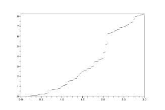
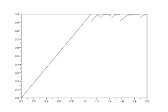
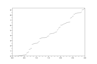
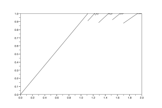
Figure 1. Two sample paths of the stochastic process $M$ built using the function $\gamma(y):=\min(1/2+y/4,0.9)$. On the right hand-side are plotted the theoretical spectra $D_{M}([0,3],.)$.

As can be seen from the definition of the local multifractal spectrum, in order to prove Theorem 6, it is enough to show (46). Indeed, (43) simply follows from considering the limit of (46) when the interval $I$ is the centered ball $B(t,r)$ and letting $r$ tend to zero.

Formula (46) is better understood when plotted: for every $s\in I\cap{\mathcal{J}}$, plot a segment whose endpoints are $(0,0)$ and $(1/\gamma(M_{s-}),1)$ (open on the right), and take the supremum to get $D_{M}(I,.)$. Sample paths of the process $M$ and their associated spectra are given in Figure 1.

The formulae giving the local and global spectra are based on the computation of the pointwise Hölder exponents at all times $t$. The value of the pointwise Hölder exponent of $M$ at $t$ depends on two parameters: the value of the process $M$ in the neighborhood of $t$, and the approximation rate of $t$ by the set of jumps ${\mathcal{J}}$. In particular, the following properties holds a.s.,

for every $$t\geq 0 h_{M}(t)\leq 1/\gamma(M_{t}),$$,

for Lebesgue-almost every $$t h_{M}(t)=1/\gamma(M_{t}),$$,

for every $$\kappa\in(0,1) \dim_{H}\{t\geq 0:\;h_{M}(t)=\kappa/\gamma(M_{t})\}=\kappa.$$,

The relevance of the local spectrum in this context is thus obvious: depending on the local value of $M$, the pointwise Hölder exponents change, and so is the (local) multifractal spectrum.

It is worth emphasizing that, as expected from the construction of the process $M$, the local spectrum (43) at any point $t>0$ essentially coincides with that of a stable Lévy subordinator of index $\gamma(M_{t})$. This local comparison is strengthened by the following theorem, which proves the existence of tangent processes for $M$ (which are Lévy stable subordinators).

Proposition 11.

We denote by $\mathcal{F}_{t}:=\sigma(\{N(A),A\in\mathcal{B}([0,t]\times[0,\infty))\})$. Let $t_{0}\geq 0$ be fixed. Conditionally on $\mathcal{F}_{t_{0}}$, the family of processes $\displaystyle\Big{(}\frac{M_{t_{0}+\alpha t}-M_{t_{0}}}{\alpha^{1/\gamma(M_{t_{0}})}}\Big{)}_{t\in[0,1]}$ converges in law, as $\alpha\to 0^{+}$, to a stable Lévy subordinator with Lévy measure $\gamma(M_{t_{0}})u^{-1-\gamma(M_{t_{0}})}du$. Here the Skorokhod space of càdlàg functions on $[0,1]$ is endowed with the uniform convergence topology.

Observe that for all $s\in{\mathcal{J}}$, all $h\in(1/\gamma(M_{s}),1/\gamma(M_{s-})]$, $d_{M}(h)=h\cdot\gamma(M_{s-})$. Thus the spectrum $d_{M}$ of $M$ on an interval $I$ is a straight line on all segments of the form $(1/\gamma(M_{s}),1/\gamma(M_{s-})]$, $s\in{\mathcal{J}}\cap I$. By the way, this spectrum, when viewed as a map from $\mathbb{R}_{+}$ to $\mathbb{R}_{+}$, is very irregular, and certainly multifractal itself. This is in sharp contrast with the spectra usually obtained, which are most of the time concave or (piecewise) real-analytic. Hence, the difference between the global and the local multifractal spectra is stunning: While $d_{M}$ is very irregular, $d_{M}(t,\cdot)$ is a straight line.

This example naturally leads to the following open problem, which would express that a natural compatibility holds for local multifractal analysis: Find general conditions under which a stochastic process $X$ which has a tangent process at a point $x_{0}$ satisfies that the multifractal spectrum of the tangent process coincides with the local spectrum of $X$ at $x_{0}$.

6. Other regularity exponents characterized by dyadic families

Other exponents than those already mentioned fit in the general framework given by Definition 7 and therefore the results supplied by multifractal analysis can be applied to them. We now list a few of them.

Pointwise Hölder regularity is pertinent only if applied to locally bounded functions. An extension of pointwise regularity fitted to functions that are only assumed to belong to $L^{p}_{loc}$ is sometimes required: The corresponding notion was introduced by Calderón and Zygmund in 1961, see [22], in order to obtain pointwise regularity results for elliptic PDEs.

Definition 17.

Let $p\in[1,+\infty)$ and $\alpha>-d/p$. Let $f\in L^{p}_{loc}(\Omega)$, and $x_{0}\in\Omega$; $f$ belongs to $T^{p}_{\alpha}(x_{0})$ if there exist $\ C>0$ and a polynomial $P$ of degree less than $\alpha$ such that, for $r$ small enough,

$$\left(\frac{1}{r^{d}}\int_{B(x_{0},r)}|f(x)-P(x-x_{0})|^{p}dx\right)^{1/p}\leq Cr^{\alpha}.$$ (47)

The $p$-exponent of $f$ at $x_{0}$ is

$$h^{p}_{f}(x_{0})=\sup\{\alpha:f\in T^{p}_{\alpha}(x_{0})\}.$$

Remarks:

• The normalization chosen in (47) is such that cusps $|x-x_{0}|^{\alpha}$ (when $\alpha\notin 2\mathbb{N}$) have an Hölder and a $p$-exponent which take the same value $\alpha$ at $x_{0}$.

• The Hölder exponent corresponds to the case $p=+\infty$.

• We only define lower exponents here: Upper exponents could also be defined in his context, by considering local $L^{p}$ norms of iterated differences.

• Definition 17 is a natural substitute for pointwise Hölder regularity when functions in $L^{p}_{loc}$ are considered. In particular, the $p$-exponent can take negative values down to $-d/p$, and typically allows to take into account behaviors which are locally of the form

  $$\frac{1}{|x-x_{0}|^{\gamma}}\;\;\mbox{ for}\;\;\gamma<d/p,$$ (48)

A pointwise regularity exponent associated with tempered distributions has been introduced by Y. Meyer: The weak scaling exponent (see [46], and also [1] for a multifractal formalism based on this exponent). It can also be interpreted as a limit case of other exponents for distributions, which can be related with the Hölder exponent; let us briefly recall how this can be done.

Let $f$ be a tempered distribution defined over $\mathbb{R}^{d}$. One can define fractional primitives of order $s$ of $f$ in the Fourier domain by

$$\widehat{f^{(-s)}}(\xi)=(1+|\xi|^{2})^{s/2}\hat{f}(\xi).$$

Since $f$ is of finite order, for $s$ large enough, $f^{(-s)}$ locally belongs to $L^{p}$ (or $L^{\infty}$). It follows that one can define regularity exponents of distributions through $p$-exponents (or Hölder exponents) of a fractional primitives of large enough order. If $f$ is only defined on a domain $\Omega$, one can still define the same exponents at $x_{0}\in\Omega$ by using a function $g\in{\mathcal{D}}(\mathbb{R}^{d})$ such that $g$ is supported inside $\Omega$ and $g(x)=1$ in a neighborhood of $x_{0}$; then $fg$ is a tempered distribution defined on $\mathbb{R}^{d}$ and the exponents of $(fg)^{(-s)}$ at $x_{0}$ clearly do not depend on the choice of $g$.

Let $f$ be a tempered distribution defined on a open domain. Denote by $h^{s}_{f}(x)$ the Hölder exponent of $f^{(-s)}$ (which is thus canonically well defined for $s$ large enough. By definition, the weak scaling exponent of $f$ at $x$ is

$${\mathcal{W}}_{f}(x)=\lim_{s\rightarrow+\infty}\left(h^{s}_{f}(x)-s\right)$$

(note that the limit always exists because the quantity considered is an increasing function of $s$). We will not deal directly with this exponent because it does not directly fit in the framework given by Definition 7. But we will rather consider the following intermediate framework.

Definition 18.

Let $f$ be a tempered distribution defined on a non-empty open set $\Omega\subset\mathbb{R}^{d}$. Let $p\geq 1$ and $s$ be large enough so that $f^{(-s)}$ belongs to $L^{p}$ in a neighborhood of $x_{0}$. The fractional $p$-exponent of order $s$ of $f$ at $x_{0}$ is defined by

$$~h^{p,s}_{f}(x_{0})=h^{p}_{f^{(-s)}}(x_{0})$$

(using the convention $h^{\infty}_{f}=h_{f}$).

Note that, in practice, the standard way to perform the multifractal analysis of data that are not locally bounded is to deal with the exponent $h^{\infty,s}_{f}$, where $s$ is chosen large enough so that $f^{(-s)}\in L^{\infty}_{loc}$, i.e. it consists in first performing a fractional integration, and then a standard multifractal analysis based on the Hölder exponent, see [2] and references therein.

Similarly, in the function case, if the pointwise regularity exponents are small enough, they can be recovered for the oscillation of $f$. Recall that the oscillation of $f$ of order $l$ on a convex set $A$ is defined through conditions on the finite differences of the function $f$, denoted by $\Delta^{M}_{h}f$: The first order difference of $f$ is

$$(\Delta_{h}^{1}f)(x)=f(x+h)-f(x).$$

If $l>1$, the differences of order $l$ are defined recursively by

$$(\Delta^{l}_{h}f)(x)=(\Delta^{l-1}_{h}f)(x+h)-(\Delta^{l-1}_{h}f)(x).$$

Then

$${\mathcal{O}}sc^{l}_{f}(A)=\sup_{x,x+lh\in A}\left|(\Delta^{l}_{h}f)(x)\right|.$$

One easily checks that the Hölder exponent can be derived for the oscillation on the cubes $3\lambda$. Let $f$ be locally bounded on an open set $\Omega$.

If $l>h_{f}(x_{0})$, then

$$\forall x_{0}\in\Omega,\hskip 28.45274pth_{f}(x_{0})=\liminf_{j\rightarrow+\infty}\frac{\log{\mathcal{O}}sc^{l}_{f}(3\lambda_{j}(x_{0}))}{\log\,2^{-j}}.$$ (49)

Recall also Proposition 3 which allows to derive numerically the Hölder exponent by a log-log plot regression bearing on the the $d_{\lambda_{j}(x_{0})}$ when $j\rightarrow+\infty$, see [34].

However, in contradistinction with the measure case, a similar formula does not hold for the upper Hölder exponent, see [23] where partial results in this direction and counterexamples are worked out.

We now turn to the wavelet characterization of the $p$-exponent. We will assume that $f$ locally belongs to $L^{p}$, with slow $L^{p}$-increase, i.e. satisfies

$$\exists C,N>0\hskip 28.45274pt\int_{\Omega\cap B(0,R)}|f(x)|^{p}dx\leq C(1+|R|)^{N}.$$

In the following, when dealing with the $T^{p}_{\alpha}$ regularity of a function $f$, we will always assume that, if $f$ is defined on an unbounded set $\Omega$, then it has slow $L^{p}$-increase, and, if $\Omega\neq\mathbb{R}^{d}$, then the wavelet basis used is compactly supported.

Definition 19.

Let $f\in L^{p}_{loc}(\Omega)$, and let $\psi_{\lambda}$ be a given wavelet basis. The local square function of $f$ is

$$S_{f,\lambda}(x)=\left(\sum_{\lambda^{\prime}\subset 3\lambda}|c_{\lambda^{\prime}}|^{2}1_{\lambda^{\prime}}(x)\right)^{1/2},$$

and the $p$-leaders are defined by $d^{p}_{\lambda}=2^{dj/p}\parallel S_{f,\lambda}\parallel_{p}.$

The following result of [36] yields a wavelet characterization of the $p$-exponent which is similar to (14).

Proposition 12.

Let $p\in(1,\infty)$ and $f\in L^{p}$. Assume that the wavelet basis used is $r$-smooth with $r>h^{p}_{f}(x_{0})+1$. Then

$$h^{p}_{f}(x_{0})=\liminf_{j\rightarrow+\infty}\frac{\log d^{p}_{\lambda_{j}(x_{0})}}{\log\,2^{-j}}.$$ (50)

Recall that the “almost-diagonalization” principle for fractional integrals on wavelet bases states that, as regards Hölder regularity, function spaces or scaling functions, one can consider that a fractional integration just acts as if it were diagonal on a wavelet basis, with coefficients $2^{-sj}$ on $\psi_{\lambda}$. This rule of thumb is justified by the fact that a fractional integration actually is the product of such a diagonal operator and of an invertible Calderon-Zygmund operator $A$ such that $A$ and $A^{-1}$ both belong to the Lemarié algebras ${\mathcal{M}}^{\gamma}$, for a $\gamma$ arbitrarily large (and which depends only on the smoothness of the wavelet basis) see [44, 45] for the definition of the Lemarié algebras and for the result concerning function spaces and [34] and references therein for Hölder regularity, function spaces or scaling functions.

It follows from Proposition 12 , and the “almost-diagonalization” principle for fractional integrals on wavelet bases, that the exponent $h^{p,s}_{f}(x_{0})$ can be obtained as follows.

Corollary 7.

Let $p\in(1,\infty)$ and $f\in L^{p}$. Let

$$S^{s}_{f,\lambda}(x)=\left(\sum_{\lambda^{\prime}\subset 3\lambda}|2^{-sj^{\prime}}c_{\lambda^{\prime}}|^{2}1_{\lambda^{\prime}}(x)\right)^{1/2}\;\;\mbox{ and}\;\;\;\;d^{p,s}_{\lambda}=2^{dj/p}\parallel S^{s}_{f,\lambda}\parallel_{p}.$$

Then, if the wavelet basis is $r$-smooth with $r>h^{p}_{f}(x_{0})+s+1$, then

$$h^{p,s}_{f}(x_{0})=\liminf_{j\rightarrow+\infty}\frac{\log d^{p,s}_{\lambda_{j}(x_{0})}}{\log\,2^{-j}}.$$ (51)

7. A functional analysis point of view

7.1. Function space interpretation: Constant regularity

If $p>0$, the scaling function has a function space interpretation, in terms of discrete Besov spaces which we now define. Recall that the elements of a dyadic family are always non-negative.

Definition 20.

Let $s\in\mathbb{R}$ and $p\in\mathbb{R}$. A dyadic function ${\mathcal{E}}$ belongs to ${\bf b}^{s,\infty}_{p}(\Omega)$ if

$$\exists C,\;\forall j,\hskip 28.45274pt2^{-dj}{\sum_{\lambda\in\Lambda^{\Omega}_{j}}}^{\ast}(e_{\lambda})^{p}\leq C\cdot 2^{-spj}.$$ (52)

If $p=+\infty$, a dyadic function ${\mathcal{E}}$ belongs to ${\bf b}^{s,\infty}_{\infty}(\Omega)$ if

$$\exists C\;\forall\lambda:\hskip 11.38109pte_{\lambda}\leq C\cdot 2^{-sj}.$$ (53)

Note that, if $p>0$, this condition (if applied to the moduli of the coefficients) defines a vector space. It is a Banach space if $p\geq 1$, and a quasi-Banach space if $0<p<1$; recall that, in a quasi-Banch space, the triangular inequality is replaced by the weaker condition :

$$\exists C,\;\forall x,y,\hskip 28.45274pt\parallel x+y\parallel\leq C(\parallel x\parallel+\parallel y\parallel).$$

Definition 20 yields a function space interpretation to the scaling function when $p>0$. It is classical in this context to rather consider the scaling function

$$\eta_{\mathcal{E}}(p)=\tau_{\mathcal{E}}(p)-d.$$

Then, if $\Omega$ is a bounded set,

$$\forall p\in\mathbb{R},\hskip 28.45274pt\eta_{{\mathcal{E}}}^{\Omega}(p)=\sup\{s:{\mathcal{E}}\in{\bf b}^{s/p,\infty}_{p}(\Omega)\};$$

and, if $\Omega$ is unbounded, then the function space interpretation is the same, using the precaution supplied by (19). Additionally,

$${h^{\Omega}_{\mathcal{E}}}=\sup\left\{s:{\mathcal{E}}\in{\bf b}^{s,\infty}_{\infty}(\Omega)\right\}.$$

The terminology of “discrete Besov spaces” is justified by the fact that, if the $e_{\lambda}$ are wavelet coefficients, then (52) and (53) are the wavelet characterization of the “classical” Besov spaces $B^{s,\infty}_{p}(\mathbb{R}^{d})$ of functions (or distributions) defined on $\mathbb{R}^{d}$; therefore each wavelet decomposition establishes an isomorphism between the space ${\bf b}^{s,\infty}_{p}(\mathbb{R}^{d})$ and the space $B^{s,\infty}_{p}(\mathbb{R}^{d})$, see [44]. Note that, when $p=\infty$, these Besov spaces coincide with the Hölder spaces $C^{s}(\mathbb{R}^{d})$, so that, when the $(e_{\lambda})$ are wavelet coefficients, then the uniform regularity exponent has the following interpretation

$${h^{\Omega}_{\mathcal{E}}}=\sup\{s:{\mathcal{E}}\in C^{s}(\mathbb{R}^{d})\}.$$

In the measure case, H. Triebel showed that the discrete Besov conditions bearing on the $\mu(3\lambda)$ can also be related with the Besov regularity of the measure $\mu$, see [59]:

$$\mbox{ If }s<d,\hskip 22.76219pt(\mu(3\lambda))\in{\bf b}^{s,\infty}_{p}(\mathbb{R}^{d})\Longleftrightarrow\mu\in B^{s-d,\infty}_{p}(\mathbb{R}^{d}).$$

In the case where $p=+\infty$, uniform regularity gives an important information concerning the sets $A$ such that $\mu(A)>0$, as a consequence of the mass distribution principle, see Section 2: Since this estimate precisely means that the sequence $(e_{\lambda})=(\mu(3\lambda))$ belongs to ${\bf b}^{s,\infty}_{\infty}(\Omega)$, it follows that, if $A\subset\Omega$ and if a measure $\mu$ satisfies $\mu(A)>0$, then

$$\dim(A)\geq h^{\Omega}_{\mu}.$$ (54)

When the sequence ${\mathcal{E}}$ is composed of wavelet leaders, or of $p$-leaders, the corresponding function spaces are no more Besov spaces, but alternative families of function spaces, the Oscillation Spaces, see [33, 35].

$${h^{\Omega}_{\mathcal{E}}}=\sup\{A:(\ref{defab})\;\mbox{ holds}\}.$$

The following upper bounds for dimensions are classical for measures, see [20], and are stated in the general setting of dyadic functions in [37].

Proposition 13.

Let ${\mathcal{E}}$ be a dyadic function, and let

$$J^{\Omega}_{H}=\{x\in\Omega:\;h_{\mathcal{E}}(x)\geq H\},\hskip 2.84526ptG^{\Omega}_{H}=\{x\in\Omega:\;h_{\mathcal{E}}(x)\geq H\},$$

$$F^{\Omega}_{H}=\{x\in\Omega:\;\tilde{h}_{\mathcal{E}}(x)\leq H)\},\hskip 2.84526ptK^{\Omega}_{H}=\{x\in\Omega:\;\tilde{h}_{\mathcal{E}}(x)\leq H)\}.$$

• If ${\mathcal{E}}\in{\bf b}^{s,\infty}_{p}(\Omega)$ with $p>0$, then $\dim(G^{\Omega}_{H})\leq d-sp+Hp$.

• If ${\mathcal{E}}\in{\bf\tilde{b}}^{s,\infty}_{p}(\Omega)$ with $p>0$, then $\dim_{p}(F^{\Omega}_{H})\leq d-sp+Hp$.

• If ${\mathcal{E}}\in{\bf b}^{s,\infty}_{p}(\Omega)$ with $p<0$, then $\dim(K^{\Omega}_{H})\leq d-sp+Hp$.

• If ${\mathcal{E}}\in{\bf\tilde{b}}^{s,\infty}_{p}(\Omega)$ with $p<0$, then $\dim_{p}(J^{\Omega}_{H})\leq d-sp+Hp$.

7.2. Function space interpretation: Varying regularity

Recall that the global scaling function has a function space interpretation in terms of Besov spaces which contain the dyadic function ${\mathcal{E}}$. Similarly, the local scaling function can be given two functional interpretations; one is local, and in terms of germ spaces at a point, and the second is global, and is in terms of function spaces with varying smoothness. We now recall these notions, starting with germ spaces in a general, abstract setting.

Definition 21.

Let $E$ be a Banach space (or a quasi-Banach space) of distributions satisfying ${\mathcal{D}}\hookrightarrow E\hookrightarrow{\mathcal{D}^{\prime}}$. Let $x\in\mathbb{R}^{d}$; a distribution $f$ belongs to $E$ locally at $x$ if there exists $\varphi\in D$ such that $\varphi(x)=1$ in a neighbourhood of $x$ and $f\varphi\in E$. We also say that $f$ belongs to the germ space of $E$ at $x$, denoted by $E_{x}$.

Let us draw the relationship between the local scaling function and germ spaces: If the $(e_{\lambda})$ are the wavelet coefficients of a function $f$, then

$$\forall p>0,\hskip 28.45274pt\eta_{f}(x,p)=\sup\left\{s:f\in B^{s/p,\infty}_{p,x}\right\}.$$

Note that, in the wavelet case, these local Besov regularity indices have been investigated by H. Triebel, see Theorem 4 of [60] where their wavelet characterization is derived, (the reader should be careful that what is referred to as “pointwise regularity” in the terminology introduced by H. Triebel is called here “local regularity”).

The uniform exponent can also be reformulated in terms of of Hölder spaces:

$$~{\mathcal{H}}_{f}(x)=\sup\left\{s:f\in C^{s}_{x}\right\}.$$

In that case, the function $~{\mathcal{H}}_{f}(x)$ is called the Local Hölder exponent of $f$. Its properties have been investigated by S. Seuret and his collaborators, see e.g. [42].

Note that the definition of germ spaces can be adapted to the dyadic functions setting.

Definition 22.

Let $E$ be a Banach space (or a quasi-Banach space) defined on dyadic functions over $\Omega$ ; a dyadic function $(e_{\lambda})$ belongs to $E_{x}$ if there exists a neighbourhood $\omega$ of $x$ such that the dyadic function $(e_{\lambda})$ restricted to $\omega$ belongs to $E$.

It is clear that this definition, when restricted to the case of Besov spaces and wavelet coefficients coincides with Definition 21.

We now turn to function spaces with varying smoothness. Such spaces were initially introduced by Unterberger and and Bokobza in [61, 62], followed by many authors (see [52] for an extensive review on the subject). A general way to introduce such spaces is to remark that the classical Sobolev spaces $H^{s,p}(\mathbb{R}^{d})$ can be defined by the condition

$$\parallel T(f)\parallel_{p}<\infty,$$

where $T$ is the pseudo-differential operator defined by

$$(Tf)(x)=\frac{1}{(2\pi)^{d}}\int_{\mathbb{R}^{d}}e^{ix\xi}(1+|\xi|^{2})^{s/2}\hat{f}(\xi)d\xi.$$

This definition leads to operators with constant order $s$ because the symbol $(1+|\xi|^{2})^{s/2}$ is independent of $x$. However, one can define more general spaces, with possibly varying order if replacing $(1+|\xi|^{2})^{s/2}$ by a symbol $\sigma(x,\xi)$. In particular the symbols $(1+|\xi|^{2})^{a(x)/2}$ will lead to Sobolev spaces of varying order $H^{a,p}$ where we can expect that, if $a$ is a smooth enough function (say continuous), then the local order of smoothness at $x$ will be $a(x)$. This particular case, and its extensions in the Besov setting, has been studied by H.G. Leopold, followed by J. Schneider, Besov, H. Triebel, A. Almeida, P. Hästö, J. Vybíral, and several other authors, who gave alternative characterizations of these space in terms of finite differences or Littlewood-Paley decomposition. They also studied their mutual embeddings (and also in the case where both the order of smoothness and the order of integrability $p$ vary) and their interpolation properties, see [53, 54] fand references therein, and also [52] for an historical account. The reader can also consult [3, 63] for recent extensions in particular when both the order of smoothness and the order of integrability $p$ vary. We follow here the presentation of J. Schneider, since this author obtained Littlewood-Paley characterizations, which are clearly equivalent to the wavelet characterization that we now give. For the sake of simplicity, we assume form now on that the distributions considered are defined on $\mathbb{R}^{d}$ and that the wavelet basis used belongs to the Schwartz class (the usual adaptations are standard in the case of functions on a domain, or for wavelets with limited regularity). We additionally assume that the function $a$ is uniformly continuous and satisfies

$$\exists c,C>0,\;\forall x\in\mathbb{R}^{d},\hskip 28.45274ptc\leq a(x)\leq C.$$ (55)

Then the Besov space $B^{a,q}_{p}$ (for $p,q\in(0,\infty]$) can be characterized by the following wavelet condition, which is independent of the wavelet basis used.

Proposition 14.

Let $a$ be a uniformly continuous function satisfying (55), and let $p,q\in(0,\infty]$. The Besov space of varying order $B^{a,q}_{p}$ is characterized by the following condition:

Let $c_{\lambda}$ denote the wavelet coefficients of a distribution $f$, and let

$$a_{j}=\left(2^{-dj}\sum_{\lambda\in\Lambda_{j}}(c_{\lambda}2^{a(\lambda)j})^{p}\right)^{1/p},$$

where $a(\lambda)$ denotes the average of the function $a$ on the cube $\lambda$; then $f\in B^{a,q}_{p}$ if $(a_{j})\in l^{q}$.

Note that when $p=q=2$ one recovers the Sobolev space $H^{a,2}$ defined above, and when $a$ is a constant equal to $s$, then one recovers the standard Besov space $B^{s,q}_{p}$. Furthermore, the embeddings

$$B^{a,1}_{p}\hookrightarrow H^{a,p}\hookrightarrow B^{a,\infty}_{p}$$

yield easy to handle “almost characterizations” of Sobolev spaces of varying order.

The following result, which follows directly from the definition of the local scaling function (Definition 8) and the characterization supplied by Proposition 14, gives the interpretation of the local scaling function in terms Besov spaces of varying order.

Proposition 15.

Let $f$ be a distribution defined on $\mathbb{R}^{d}$. Then, for $p>0$, the local wavelet scaling function of $f$ can be recovered by

$$\forall p>0,\hskip 28.45274pt\eta_{f}(p,x)=p\cdot\sup\{a:f\in B^{a,\infty}_{p}\}.$$

Acknowledgement:

This work is supported by the ANR grants AMATIS and MUTATIS and by the LaBeX Bézout. The last two authors thank M. Lapidus for his kind invitation to the fractal geometry session in the AMS conference, March 2012.

References

- [1] P. Abry, S. Jaffard and Lashermes, B., Wavelet leaders in multifractal analysis : In: Qian, T., et al. 1046 (eds.) Wavelet Analysis and Applications,. Applied and Numerical Harmonic Analysis, pp. 201–246 Birkhäuser Verlag, Basel, Switzerland (2006)
- [2] P. Abry, S. Jaffard and H. Wendt, Irregularities and scaling in signal and Image processing: Multifractal analysis, to appear in: M. Frame Ed., Benoit Mandelbrot: A Life in Many Dimensions, World Scientific, 2012.
- [3] A. Almeida and P. Hästö, Besov spaces with variable smoothness and integrability, J. Funct. Anal Vol. 258 n. 5, 1628–1655, 2010.
- [4] A. Arneodo, B. Audit, N. Decoster, J.-F. Muzy, C. Vaillant, Wavelet-based multifractal formalism: applications to DNA sequences, satellite images of the cloud structure and stock market data, in: The Science of Disasters; A. Bunde, J. Kropp, H. J. Schellnhuber Eds., Springer pp. 27–102 (2002).
- [5] J.-M. Aubry and S. Jaffard, Random wavelet series, Comm. Math. Phys. 227(3):483–514, 2002.
- [6] A. Ayache and M. S. Taqqu, Multifractional processes with random exponent, Publ. Mat. 49(2):459–486, 2005.
- [7] A. Ayache, S. Jaffard, and M. S. Taqqu, Wavelet construction of generalized multifractional processes, Rev. Mat. Iberoam. 23(1):327–370, 2007.
- [8] I.-S. Baek, Hausdorff dimension of deranged Cantor set without some boundedness condition, Comm. Korean Math. Soc. 1:113–117, 2004.
- [9] J. Barral, N. Fournier, S. Jaffard, and S. Seuret, A pure jump Markov process with a random singularity spectrum, Ann. Probab. 38(5):1924–1946, 2010.
- [10] J. Barral, J. Berestycki, J. Bertoin, A. Fan, B. Haas, S. Jaffard, G. Miermont, and J. Peyrière. Quelques interactions entre analyse, probabilités et fractals. S.M.F., Panoramas et synthèses 32, 2010.
- [11] J. Barral, F. Ben Nasr, J. Peyrière, Comparing the multifractal formalisms: the neighboring boxes condition, Asian J. Maths, 7 (2003), 149–165.
- [12] J. Barral and B. Mandelbrot, Non-degeneracy, moments, dimension, and multifractal analysis for random multiplicative measures (Random multiplicative multifractal measures, Part II), pp 17–52, In Proc. Symp. Pures Math., 72, Part 2. AMS, Providence, RI (2004).
- [13] J. Barral and S. Seuret, Function series with multifractal variations, Math. Nachr., 274-275 (2) 3-18, 2004.
- [14] J. Barral and S. Seuret, Combining multifractal additive and multiplicative chaos, Commun. Math. Phys., 257 (2), 473-497, 2005
- [15] J. Barral, S. Seuret: The singularity spectrum of Lévy processes in multifractal time, Adv. Math., 214 (2007), 437–468.
- [16] J. Barral and S. Seuret, The multifractal nature of heterogeneous sums of Dirac masses, Math. Proc. Cambridge Philos. Soc., 144 (3) 707-727, 2008.
- [17] J. Barral and S. Seuret, Information parameters and large deviations spectrum of discontinuous measures, Real Analysis Exchange, 32 (2) 429-454, 2007.
- [18] J. Barral, Y. Qu, Multifractal analysis of and localized asymptotic behavior for almost additive potentials, Discr. Cont. Dynam. Sys. A, 32 (2012), 717–751.
- [19] A. Benassi, S. Jaffard, and D. Roux, Elliptic Gaussian random processes, Rev. Mat. Iberoamericana 13(1):19–90, 1997.
- [20] G. Brown, G. Michon and J. Peyrière, On the multifractal analysis of measures, J. Statist. Phys., vol. 66 pp. 775-790 (1992).
- [21] Z. Buczolich, S. Seuret, Measures and functions with prescribed homogeneous multifractal spectrum, Preprint, 2012.
- [22] A.-P. Calderón and A. Zygmund, Local properties of solutions of elliptic partial differential equations, Studia Math. 20:171–225, 1961.
- [23] M. Clausel, S. Nicolay, Wavelets techniques for pointwise anti-Holderian irregularity, Constr. Approx., 33:41–75, 2011.
- [24] A. Durand, Singularity sets of Lévy processes, Probab. Theory Relat. Fields 143(3-4):517–544, 2009.
- [25] A. Durand and S. Jaffard, Multifractal analysis of Lévy fields, Probab. Theory Relat. Fields, Vol. 153 pp. 45–96, 2012.
- [26] K. Falconer, Sets with large intersection properties, J. London Math. Soc. (2) 49(2):267–280, 1994.
- [27] K. Falconer, Fractal geometry: Mathematical foundations and applications, John Wiley & Sons Inc., Chichester, 2nd edition, 2003.
- [28] A. H. Fan and D. J. Feng, On the distribution of long-term time averages on symbolic space, J. Statist. Phys., 99 (2000), 813–856.
- [29] D.J. Feng, Lyapunov exponents for products of matrices and Multifractal analysis. Part II: Non-negative matrices, Israël J. Math., 170 (2009), p. 355-394.
- [30] D. J. Feng, K.S. Lau and X.-Y. Wang, Some exceptional phenomena in multifractal formalism. II., Asian J. Math. 9 (2005), p. 473–488.
- [31] D.-J. Feng, E. Olivier, Multifractal analysis of the weak Gibbs measures and phase transition- Application to some Bernoulli convolutions, Ergod. Th. Dynam. Sys., 23 (2003), 1751-1784.
- [32] S. Jaffard, The multifractal nature of Lévy processes, Probab. Theory Relat. Fields 114(2):207–227, 1999.
- [33] S. Jaffard, Oscillation spaces: Properties and applications to fractal and multifractal functions, J. Math. Phys., Vol. 39 pp. 4129–4141 (1998).
- [34] S. Jaffard, Wavelet techniques in multifractal analysis, in Fractal geometry and applications: a jubilee of Benoît Mandelbrot, Part 2, vol. 72 of Proc. Sympos. Pure Math., pages 91–151, Amer. Math. Soc., Providence, RI, 2004.
- [35] S. Jaffard, Beyond Besov spaces Part 2: Oscillation spaces, Const. Approx., Vol 21 n. 1 pp. 29-61. (2005)
- [36] S. Jaffard, Pointwise regularity associated with function spaces and multifractal analysis, Banach Center Pub. Vol. 72 Approximation and Probability, T. Figiel and A. Kamont Eds. pp. 93–110 (2006)
- [37] S. Jaffard, P. Abry, S.G. Roux, B. Vedel, and H. Wendt. The contribution of wavelets in multifractal analysis, Series in contemporary applied mathematics. World scientific publishing, pp. 51–98 (2010)
- [38] H. Jürgensen, and L. Staiger, Local Hausdorff dimension, Acta Inf. 32(5):491–507,1995.
- [39] A. Käenmäki, T. Rajala and N. Suomala, Local homogeneity and dimensions of measures in doubling metric spaces, preprint, 2012.
- [40] M. Kesseböhmer, Large deviation for weak Gibbs measures and multifractal spectra, Nonlinearity, 14 (2001), 395-409.
- [41] P. Lemarié-Rieusset and Y. Meyer, Ondelettes et bases hilbertiennes, Rev. Mat. Iberoamericana 2(1-2):1–18, 1986.
- [42] J. Lévy Véhel, S. Seuret. The local Holder function of a continuous function, Appl. Comput. Harmon. Anal., 13(3) 263–276, 2002.
- [43] J. Lévy Véhel, R. Vojak, Multifractal analysis of Choquet capacities, Adv. Appl. Math., 20 (1998), 1–43.
- [44] Y. Meyer, Ondelettes et opérateurs. Hermann, 1990.
- [45] Y. Meyer and R. Coifman, Wavelets, volume 48 of Cambridge Studies in Advanced Mathematics. Cambridge University Press, Cambridge, 1997. Calderón-Zygmund and multilinear operators, Translated from the 1990 and 1991 French originals by David Salinger.
- [46] Y. Meyer, Wavelets, Vibrations and Scalings, CRM Ser. AMS Vol. 9, Presses de l’Université de Montréal,1998.
- [47] L. Olsen, A multifractal formalism, Adv. Math. 116 (1995), p. 92–195.
- [48] N. Patzschke, Self-conformal multifractal measures, Adv. in Appl. Math., 19 (1997), no. 4, 486–513.
- [49] R. Peltier and J. Lévy-Véhel, Multifractional Brownian motion: definition and preliminary results, Tech. Rep. RR 2645, INRIA Le Chesnay, France, 1995.
- [50] Y. Pesin, Dimension theory in dynamical systems: Contemporary views and applications, Chicago lectures in Mathematics, The University of Chicago Press, 1997.
- [51] J. Schmeling, S. Seuret, On measures resisting multifractal analysis, Book chapter in the book ”Nonlinear Dynamics: New Directions” (in honor of V. Afraimovich), Springer 2012 (in press).
- [52] J. Schneider, Function spaces with varying smoothness, PhD Dissertation available on http://personal-homepages.mis.mpg.de/jschneid/Public.html 2005.
- [53] J. Schneider, Function spaces with varying smoothness I, Math. Nachr. Vol. 280 (16), 1801-1826, 2007.
- [54] J. Schneider, Some results on function spaces of varying smoothness, Proc.Funct.Sp.VIII, Banach Center Publ. Vol. 79, pp.187–195, Warszawa, 2008.
- [55] S. Seuret, On multifractality and time subordination for continuous functions, Adv. Math., 220(3) 936-963, 2009.
- [56] P. Shmerkin, A modified multifractal formalism for a class of self-similar measures with overlap, Asian J. Math. 9 (2005), p. 323–348.
- [57] B. Testud, Phase transitions for the multifractal analysis of self-similar measures, Nonlinearity 19 (2006), p. 1201–1217.
- [58] C. Tricot, Two definitions of fractional dimension, Math. Proc. Cambridge Philos. Soc, 91 (1) pp. 57–-74, 1982.
- [59] H. Triebel, Fractal characteristics of measures; an approach via function spaces, J. Four. Anal. Appl. 9, (4), 411–430, 2003.
- [60] H. Triebel, Wavelet frames for distributions; local and pointwise regularity, Stud. Math., 154 (1) pp. 59–88, 2003.
- [61] A. Unterberger and J. Bokobza Sur une généralisation des opérateurs de Calderon-Zygmund et des espaces C. R. Acad. Sci. Paris (Ser A), 260 pp. 3265–-3267, 1965.
- [62] A. Unterberger and J. Bokobza Les opérateurs pseudo-différentiels d’ordre variable C. R. Acad. Sci. Paris (Ser A), 261 pp. 2271–-2273, 1965.
- [63] J. Vybíral, Sobolev and Jawerth embeddings for spaces with variable smoothness and integrability, Ann. Acad. Sci. Fenn. Math. Vol. 34, 529–544, 2009.