Electromagnetic form factors of the nucleon
in effective field theory

Abstract

We calculate the electromagnetic form factors of the nucleon to third chiral order in manifestly Lorentz-invariant effective field theory. The $\rho$ and $\omega$ mesons as well as the $\Delta(1232)$ resonance are included as explicit dynamical degrees of freedom. To obtain a self-consistent theory with respect to constraints we consider the proper relations among the couplings of the effective Lagrangian. For the purpose of generating a systematic power counting, the extended on-mass-shell renormalization scheme is applied in combination with the small-scale expansion. The results for the electric and magnetic Sachs form factors are analyzed in terms of experimental data and compared to previous findings in the framework of chiral perturbation theory. The pion-mass dependence of the form factors is briefly discussed.

I Introduction

Electromagnetic form factors parameterize the single-nucleon matrix element of the electromagnetic current operator and provide important information about the structure and composition of the nucleon (see, e.g., Refs. Gao:2003ag ; Perdrisat:2006hj ; Drechsel:2007sq for an overview). Furthermore, they are important input to high-precision tests of quantum electrodynamics as well as the Standard Model of particle physics. In the space-like region, the proton form factors have been measured with great accuracy over a wide range of momentum transfer in experiments on elastic electron-nucleon scattering. Neutron form factors are not as well known since they have to be extracted from scattering experiments with deuterium or ${}^{3}\textrm{He}$. Despite the wealth of the available data there are still open issues such as the value of the proton charge radius determined from the Lamb shift in muonic hydrogen on the one hand Mohr:2012tt and electronic hydrogen Lamb shift measurements and elastic electron-proton scattering on the other hand Beringer:1900zz . A new generation of precision measurements of electromagnetic form factors at low momentum transfer has been and is presently performed at the Mainz Microtron MAMI Bernauer:2008zz ; Bernauer:2010wm .

Chiral perturbation theory (ChPT) Weinberg:1978kz ; Gasser:1983yg ; Gasser:1987rb is the effective field theory (EFT) of quantum chromodynamics in the low-energy domain (for an introduction and review see, e.g., Refs. Scherer:2009bt ; Scherer:2012zzd ). The first form factor calculation was performed in the early relativistic approach Gasser:1987rb , in which, however, the power counting of low-energy dimensions was still an open issue due to the additional heavy-mass scale introduced by the nucleon. Later on, the problem of setting up a consistent power counting in EFT with heavy degrees of freedom was handled by employing the heavy-baryon approach Jenkins:1990jv ; Bernard:1992qa and, more recently, by choosing suitable renormalization prescriptions in a manifestly Lorentz-invariant framework Tang:1996ca ; Becher:1999he ; Gegelia:1999gf ; Fuchs:2003qc . Within the heavy-baryon approach, calculations of the form factors were performed in Refs. Bernard:1992qa ; Fearing:1997dp and, including the $\Delta(1232)$ resonance in terms of the small-scale expansion Hemmert:1997ye , in Ref. Bernard:1998gv . Applying different renormalization schemes, form factor calculations have been performed within manifestly Lorentz-invariant baryon ChPT up to $\mathcal{O}(q^{4})$ Kubis:2000zd ; Fuchs:2003ir and to $\mathcal{O}(q^{3})$ including the leading-order corrections due to the $\Delta$ resonance Ledwig:2011cx . In general, such calculations describe the experimental data only for a small range of momentum transfer ($Q^{2}\leq 0.1~{}\textrm{GeV}^{2}$). On the other hand, the $\rho$, $\omega$, and $\phi$ mesons were included dynamically in the effective Lagrangians of Refs. Kubis:2000zd ; Schindler:2005ke . A systematic re-summation of higher-order terms which, in an ordinary chiral expansion, would contribute at higher orders beyond ${\cal O}(q^{4})$, results in an improved description of the data even for higher values of $Q^{2}$, as expected on phenomenological grounds. The re-organization proceeds according to well-defined rules FSGS03 so that a controlled, order-by-order calculation of corrections is made possible.

A covariant formalism for massive vector fields involves Lagrangians with constraints, because one typically introduces unphysical degrees of freedom weinbergQTFI . In comparison with Refs. Kubis:2000zd ; Schindler:2005ke , the present paper considers the conditions on the form of the Lagrangian imposed by the demand for a self-consistent theory in terms of constraints Djukanovic:2004mm ; Djukanovic:2010tb . We use the extended on-mass-shell (EOMS) scheme Fuchs:2003qc to generate a systematic power counting in the presence of heavy degrees of freedom FSGS03 . As a result, we obtain an effective Lagrangian which is renormalizable in the sense of effective field theory weinbergQTFIb and which is consistent with the constraints order by order.

Because of its close proximity to the ground state and its strong coupling to the pion-nucleon-photon system we also include the $\Delta(1232)$ resonance explicitly in our effective theory. The nucleon-$\Delta$ mass splitting is treated as an additional small parameter (small-scale expansion Hemmert:1997ye ). Akin to the vector-meson case we respect the constraints on the possible interaction terms to obtain a self-consistent theory describing the right number of degrees of freedom Wies:2006rv ; Hacker:2005fh .

This paper is organized as follows. In Sec. II the definitions of the Dirac and Pauli as well as the Sachs form factors are given. We briefly discuss those elements of the most general effective Lagrangian relevant for the subsequent calculation and state the applied power-counting rules in Sec. III. In Sec. IV we discuss the fit of our results to experimental data. The final results for the Sachs form factors are presented and analyzed. Section V contains a short summary.

II Electromagnetic Form Factors of the Nucleon

Neglecting the contributions due to heavier quarks, the electromagnetic current operator is given by

$$J^{\mu}(x)=\frac{2}{3}\bar{u}(x)\gamma^{\mu}u(x)-\frac{1}{3}\bar{d}(x)\gamma^{\mu}d(x)=\bar{q}(x)\left(\frac{1}{6}+\frac{\tau_{3}}{2}\right)\gamma^{\mu}q(x),$$ (1)

and the interaction with an external electromagnetic four-vector potential $\mathcal{A}_{\mu}$ reads

$$\mathcal{L}_{\textrm{e.m.}}=-eJ^{\mu}\mathcal{A}_{\mu},$$ (2)

where $e>0$ denotes the elementary charge. In the one-photon-exchange approximation, the electromagnetic form factors are defined via the matrix element

$$\langle{N(p_{f})}|J^{\mu}(0)|{N(p_{i})}\rangle=\bar{u}(p_{f})\left[\gamma^{\mu}F_{1}^{N}(Q^{2})+\frac{i\sigma^{\mu\nu}q_{\nu}}{2m_{p}}F_{2}^{N}(Q^{2})\right]u(p_{i}),\qquad N=p,n,$$ (3)

where $m_{p}$ denotes the proton mass, $q=p_{f}-p_{i}$ is the four-momentum transfer, and $Q^{2}\equiv-q^{2}\geq 0$. The functions $F_{1}^{N}(Q^{2})$ and $F_{2}^{N}(Q^{2})$ are called Dirac and Pauli form factors, respectively. At $Q^{2}=0$, the Dirac form factor takes the value of the electric charge in units of the elementary charge and the Pauli form factor takes the value of the anomalous magnetic moment in units of the nuclear magneton:

$$F_{1}^{p}(0) =1,\qquad F_{2}^{p}(0)=1.793,$$ (4)

$$F_{1}^{n}(0) =0,\qquad F_{2}^{n}(0)=-1.913.$$ (5)

Our final results will be displayed in terms of the electric and magnetic Sachs form factors Ernst:1960zza since these are better suited for the analysis of experimental data. The Sachs form factors are related to the Dirac and Pauli form factors as follows:

$$\begin{split}G_{E}^{N}(Q^{2})&=F_{1}^{N}(Q^{2})-\frac{Q^{2}}{4m_{p}^{2}}F^{N}_{2}(Q^{2}),\\ G_{M}^{N}(Q^{2})&=F_{1}^{N}(Q^{2})+F^{N}_{2}(Q^{2}).\end{split}$$ (6)

Sometimes it is more convenient to work with the isoscalar and isovector form factors defined as the sum and difference of the proton and neutron form factors, respectively,

$$F_{i}^{(s)}=F_{i}^{p}+F_{i}^{n},\quad F_{i}^{(v)}=F_{i}^{p}-F_{i}^{n},\quad i=1,2.$$ (7)

The isoscalar and isovector Sachs form factors are defined accordingly.

III Effective Lagrangian and power counting

III.1 Non-resonant Lagrangian

The non-resonant part of the effective Lagrangian consists of a purely mesonic part and a part describing the interaction of pions and nucleons. From the mesonic sector only the lowest-order Lagrangian ${\cal L}_{2}$, including the coupling to an external electromagnetic four-vector potential $\mathcal{A}_{\mu}$ in terms of the isovector field $v_{\mu}=-e\mathcal{A}_{\mu}\tau_{3}/2$, is needed Gasser:1983yg ,

$${\cal L}_{2}=\frac{F^{2}}{4}\textrm{Tr}\left(\partial_{\mu}U\partial^{\mu}U^{\dagger}\right)+\frac{F^{2}M^{2}}{4}\textrm{Tr}\left(U^{\dagger}+U\right)+i\frac{F^{2}}{2}\textrm{Tr}\left[(\partial^{\mu}UU^{\dagger}+\partial^{\mu}U^{\dagger}U)v_{\mu}\right].$$ (8)

Here, $F$ denotes the pion-decay constant in the chiral limit, $F_{\pi}=F\left[1+\mathcal{O}(\hat{m})\right]=92.2$ MeV, and $M^{2}=2B\hat{m}$ is the squared pion mass at leading order in the quark-mass expansion. In the isospin-symmetric limit $\hat{m}=m_{u}=m_{d}$, and $B$ is related to the scalar singlet quark condensate $\left\langle\bar{q}q\right\rangle_{0}$ in the chiral limit Gasser:1983yg ; Colangelo:2001sp . The pion fields are contained in the unimodular, unitary matrix $U$:

$$U(x)=u^{2}(x)=\exp\left(i\frac{\phi(x)}{F}\right),\quad\phi=\phi_{k}\tau_{k}.$$

Collecting the proton and nucleon fields in the isospin doublet $\Psi$, the lowest-order $\pi N$ Lagrangian is given by Gasser:1987rb

$${\cal L}_{\pi N}^{(1)}=\bar{\Psi}\left(i\not{D}-m+\frac{\texttt{g}_{A}}{2}\gamma^{\mu}\gamma_{5}u_{\mu}\right)\Psi,$$ (9)

with

$$D_{\mu}\Psi =\left(\partial_{\mu}+\Gamma_{\mu}-iv_{\mu}^{(s)}\right)\Psi,$$

$$\Gamma_{\mu} =\frac{1}{2}\left[u^{\dagger}\partial_{\mu}u+u\partial_{\mu}u^{\dagger}-i\left(u^{\dagger}v_{\mu}u+uv_{\mu}u^{\dagger}\right)\right],$$

$$u_{\mu} =i\left[u^{\dagger}\partial_{\mu}u-u\partial_{\mu}u^{\dagger}-i\left(u^{\dagger}v_{\mu}u-uv_{\mu}u^{\dagger}\right)\right],$$

where $v_{\mu}^{(s)}=-e\mathcal{A}_{\mu}/2$ In Eq. (9), $m$ and $\texttt{g}_{A}$ denote the chiral limit of the physical nucleon mass and the axial-vector coupling constant, respectively.

The complete Lagrangians at second and third order can be found in Ref. Ecker:1995rk . We only display those terms needed for our calculation,

$$\begin{split}{\cal L}_{\pi N}^{(2)}&=\bar{\Psi}\sigma^{\mu\nu}\left(\frac{c_{6}}{2}f^{+}_{\mu\nu}+\frac{c_{7}}{2}v^{(s)}_{\mu\nu}\right)\Psi+\cdots\>,\\ {\cal L}_{\pi N}^{(3)}&=\frac{i}{2m}d_{6}\bar{\Psi}[D^{\mu},f^{+}_{\mu\nu}]D^{\nu}\Psi+{\rm H.c.}+\frac{2i}{m}d_{7}\bar{\Psi}\left(\partial^{\mu}v^{(s)}_{\mu\nu}\right)D^{\nu}\Psi+{\rm H.c.}+\cdots\>,\end{split}$$ (10)

where H.c. refers to the Hermitian conjugate and

$$f^{\pm}_{\mu\nu} =uf_{L\mu\nu}u^{\dagger}\pm u^{\dagger}f_{R\mu\nu}u,$$

$$f_{R\mu\nu} =\partial_{\mu}r_{\nu}-\partial_{\nu}r_{\mu}-i\left[r_{\mu},r_{\nu}\right],$$

$$f_{L\mu\nu} =\partial_{\mu}l_{\nu}-\partial_{\nu}l_{\mu}-i\left[l_{\mu},l_{\nu}\right],$$

$$v_{\mu\nu}^{(s)} =\partial_{\mu}v_{\nu}^{(s)}-\partial_{\nu}v_{\mu}^{(s)},$$

with $r_{\mu}=l_{\mu}=-e\mathcal{A}_{\mu}\tau_{3}/2$.

III.2 Lagrangian containing vector mesons

The $\rho$-meson triplet consists of a pair of charged fields, $\rho_{\mu}^{\pm}=(\rho_{1\mu}\mp i\rho_{2\mu})/\sqrt{2}$, and a third neutral field, $\rho_{\mu}^{0}=\rho_{3\mu}$. Using a covariant Lagrangian formalism, self-interacting massive vector fields are subject to constraints weinbergQTFI . It was shown in Ref. Djukanovic:2010tb that the requirement for a quantum field theory of vector mesons to be self consistent in terms of constraints and perturbative renormalizability leads to relations among the coupling constants of the Lagrangian. Eventually, at leading order the self-interacting part of the most general effective Lagrangian for $\rho$ mesons reduces to a massive Yang-Mills structure Djukanovic:2010tb ,

$${\cal L}_{\rho\>\rm eff}=-\frac{1}{2}\textrm{Tr}\left(\rho_{\mu\nu}\rho^{\mu\nu}\right)+M_{\rho}^{2}\textrm{Tr}(\rho_{\mu}\rho^{\mu}),$$ (11)

where

$$\rho_{\mu} =\rho_{k\mu}\frac{\tau_{k}}{2},$$

$$\rho_{\mu\nu} =\partial_{\mu}\rho_{\nu}-\partial_{\nu}\rho_{\mu}-ig[\rho_{\mu},\rho_{\nu}].$$

The Lagrangian of Eq. (11) contains two parameters, namely, the $\rho$-meson mass $M_{\rho}$ (in the chiral limit) and a coupling strength $g$. Under the pair of local chiral transformations $(V_{L},V_{R})$, we choose the $\rho$ mesons to transform inhomogeneously Weinberg:1968de (model III of Ref. Ecker:1989yg ),

$$\rho_{\mu}\mapsto K\rho_{\mu}K^{\dagger}-\frac{i}{g}\partial_{\mu}KK^{\dagger},$$ (12)

where

$$K(V_{L},V_{R},U)={\sqrt{V_{R}UV_{L}^{\dagger}}}^{\,-1}V_{R}\sqrt{U}.$$

Equation (12) implies $\rho_{\mu\nu}\mapsto K\rho_{\mu\nu}K^{\dagger}$. The mass term remains chirally invariant through the replacement $\rho_{\mu}\to\rho_{\mu}-(i/g)\Gamma_{\mu}$, the result of which transforms homogeneously under local chiral transformations. Neglecting terms irrelevant for the calculation of the form factors, the effective chiral Lagrangian can be written as

$${\cal L}_{\pi\rho}={} -\frac{1}{2}\textrm{Tr}\left(\rho_{\mu\nu}\rho^{\mu\nu}\right)+M_{\rho}^{2}\textrm{Tr}\left[\left(\rho_{\mu}-\frac{i}{g}\Gamma_{\mu}\right)\left(\rho^{\mu}-\frac{i}{g}\Gamma^{\mu}\right)\right]+\frac{d_{x}}{2}\textrm{Tr}\left(\rho_{\mu\nu}f_{+}^{\mu\nu}\right)+\cdots.$$ (13)

Besides the proper relations among the self couplings of the $\rho$ mesons, the Lagrangian of Eq. (13) gives rise to vector-meson dominance in the sense that, both, the $\rho\pi\pi$ and the $\rho\gamma$ coupling contained in the mass term [second term on the right-hand side of Eq. (13)] are of leading order. The $d_{x}$ term parameterizes a deviation of higher order. In model III of Ref. Ecker:1989yg it is neglected, i.e., set to zero. According to Ref. Ecker:1989yg , the Lagrangian of Eq. (13) is obtained from the most general one by performing a field redefinition and implementing certain relations among the coupling constants. These relations exactly correspond to those derived in Ref. Djukanovic:2010tb rendering Eq. (13) consistent with the constraints and renormalizable in a perturbative sense.

In addition to $\rho$ mesons, we also include the $\omega$ meson as a dynamical degree of freedom. For our calculation, from the leading-order Lagrangian Ecker:1989yg we only need the coupling of the $\omega$ meson to external fields:

$${\cal L}_{\pi\omega}^{(3)}=-f_{\omega}\left(\partial^{\mu}\omega^{\nu}-\partial^{\nu}\omega^{\mu}\right)v^{(s)}_{\mu\nu}+\cdots.$$ (14)

Finally, we require the coupling of vector mesons to the nucleon which for our purposes is given by

$${\cal L}_{\pi VN}={} \bar{\Psi}\left[g\left(\rho_{\mu}-\frac{i}{g}\Gamma_{\mu}\right)+\frac{1}{2}\>g_{\omega}\>\omega_{\mu}\>\right]\gamma^{\mu}\>\Psi+\frac{G_{\rho}}{2}\bar{\Psi}\rho_{\mu\nu}\sigma^{\mu\nu}\Psi+\cdots.$$ (15)

Here, we have applied the universality of the $\rho$-meson coupling $g_{\rho NN}=g$. In the realization of Ref. Weinberg:1968de , the universal coupling is a consequence of chiral symmetry. In the present context, it is more likely to be a consequence of consistency conditions imposed by the demand of perturbative renormalizability Djukanovic:2004mm . A coupling of the $\omega$ meson to the nucleon proportional to $\sigma^{\mu\nu}$ is not needed at third chiral order, because there is no $\omega\gamma$ coupling at leading order in Eq. (14) as opposed to the leading-order $\rho\gamma$ coupling of Eq. (13).

III.3 Lagrangian containing the $\Delta(1232)$ resonance

The $\Delta(1232)$ resonance $\left[I(J^{P})=\frac{3}{2}(\frac{3}{2}^{+})\right]$ will be described by a vector-spinor isovector-isospinor with components

$$\Psi_{\mu,i}=\left(\begin{array}[]{cc}\Psi_{\mu,i,\frac{1}{2}}\\ \Psi_{\mu,i,-\frac{1}{2}}\end{array}\right),\qquad\mu=0,1,2,3,\qquad i=1,2,3.$$

The physical $\Delta$ consists of an isospin quadruplet, whereas the description above involves six isospin components. In order to project onto the physical degrees of freedom, we introduce the isospin projection operators (see, e.g., Sec. 4.7 of Ref. Scherer:2012zzd for more details)

$$\xi^{\frac{3}{2}}_{ij,\alpha\beta} =\delta_{ij}\delta_{\alpha\beta}-\frac{1}{3}\left(\tau_{i}\tau_{j}\right)_{\alpha\beta},$$

$$\xi^{\frac{1}{2}}_{ij,\alpha\beta} =\frac{1}{3}\left(\tau_{i}\tau_{j}\right)_{\alpha\beta},$$

where the isovector components refer to a Cartesian isospin basis. Incorporating the projection operators explicitly, the leading-order Lagrangian in $n$ space-time dimensions reads Hemmert:1997ye

$${\cal L}^{(1)}_{\pi\Delta}=\bar{\Psi}_{\mu}\xi^{\frac{3}{2}}\Lambda^{(1)\mu\nu}_{\pi\Delta}(A,n)\xi^{\frac{3}{2}}\Psi_{\nu},$$ (17)

with

$$\Lambda^{(1)\mu\nu}_{\pi\Delta}(A,n)={} -\Big{\{}(i\not{D}-m_{\Delta})g^{\mu\nu}+iA(\gamma^{\mu}D^{\nu}+\gamma^{\nu}D^{\mu})$$

$$+\frac{i}{n-2}\left[(n-1)A^{2}+2A+1\right]\gamma^{\mu}\not{D}\gamma^{\nu}$$

$$+\frac{m_{\Delta}}{(n-2)^{2}}\left[n(n-1)A^{2}+4(n-1)A+n\right]\gamma^{\mu}\gamma^{\nu}$$

$$+\frac{\texttt{g}_{1}}{2}\not{u}\gamma_{5}g^{\mu\nu}+\frac{\texttt{g}_{2}}{2}(\gamma^{\mu}u^{\nu}+u^{\mu}\gamma^{\nu})\gamma_{5}+\frac{\texttt{g}_{3}}{2}\gamma^{\mu}\not{u}\gamma_{5}\gamma^{\nu}\Big{\}}.$$ (18)

Here, the covariant derivative is given by

$$\left(D_{\mu}\Psi\right)_{\nu,i,\alpha} ={\cal D}_{\mu,ij,\alpha\beta}\Psi_{\nu,j,\beta},$$

$${\cal D}_{\mu,ij,\alpha\beta} =\partial_{\mu}\delta_{ij}\delta_{\alpha\beta}-2i\epsilon_{ijk}\Gamma_{\mu,k}\delta_{\alpha\beta}+\delta_{ij}\Gamma_{\mu,\alpha\beta}-iv_{\mu}^{(s)}\delta_{ij}\delta_{\alpha\beta},$$

where we parameterized $\Gamma_{\mu}=\Gamma_{\mu,k}\tau_{k}$. In Eq. (17), $A\neq-\frac{1}{2}$ denotes an arbitrary real parameter and $m_{\Delta}$ refers to the leading-order mass of the $\Delta$.

Since the Lagrangian of Eq. (17) describes a system with constraints, similarly to the previously discussed case of vector mesons, the requirement for a self-consistent theory leads to relations among the coupling constants Wies:2006rv ,

$$\texttt{g}_{2}=A\texttt{g}_{1},\qquad\texttt{g}_{3}=-\frac{1+2A+A^{2}(n-1)}{n-2}\>\texttt{g}_{1}.$$

The lowest-order $\pi N\Delta$ interaction Lagrangian reads Hacker:2005fh ,

$${\cal L}^{(1)}_{\pi N\Delta}=\texttt{g}\bar{\Psi}_{\mu,i}\xi_{ij}^{\frac{3}{2}}\left(g^{\mu\nu}+\frac{1+3A}{2}\>\gamma^{\mu}\gamma^{\nu}\right)u_{\nu,j}\Psi+{\rm H.c.}\>,$$ (19)

with the parameterization $u_{\mu}=u_{\mu,k}\tau_{k}$, and g being a coupling constant. Since physical quantities cannot depend on $A$ Hacker:2005fh , we choose $A=-1$ in the following calculations.

III.4 Power counting

We assign a low-energy order $D$ to each renormalized diagram. The value of $D$ is determined with the following power-counting rules: A pion propagator counts as $\mathcal{O}(q^{-2})$, a nucleon propagator as $\mathcal{O}(q^{-1})$, vertices derived from ${\cal L}_{2}$ count as $\mathcal{O}(q^{2})$, and vertices from ${\cal L}_{\pi N}^{(i)}$ count as $\mathcal{O}(q^{i})$. Both $\rho$-meson and $\omega$-meson propagators count as $\mathcal{O}(q^{0})$ while vertices from ${\cal L}_{\pi\omega}^{(3)}$ count as $\mathcal{O}(q^{3})$. From the listed terms of ${\cal L}_{\pi\rho}$ and ${\cal L}_{\pi VN}$ vertices of $\mathcal{O}(q^{0})$ to $\mathcal{O}(q^{3})$ can be derived. The $\Delta$ propagator counts as $\mathcal{O}(q^{-1})$ and vertices from ${\cal L}^{(1)}_{\pi N\Delta}$ count as $\mathcal{O}(q)$. Finally, we assign the order $\mathcal{O}(q)$ to the mass difference $\delta\equiv m_{\Delta}-m$. In order to renormalize the loop diagrams in such a way that they respect the above power counting, we apply the EOMS scheme Fuchs:2003qc .

IV Results and Discussion

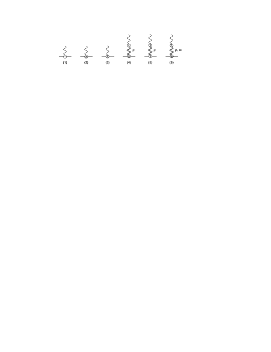
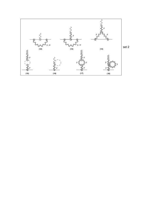
Figure 1: Feynman diagrams including vector mesons and the $\Delta$ resonance contributing to the electromagnetic form factors of the nucleon up to and including $\mathcal{O}(q^{3})$. Solid, dashed, wiggly, double-wiggly, and double-solid lines refer to nucleons, photons, pions, vector mesons, and the $\Delta$ resonance, respectively. The numbers in the interaction blobs denote the chiral order of the respective vertex.

All Feynman graphs contributing to the calculation of the electromagnetic form factors up to and including $\mathcal{O}(q^{3})$ are displayed in Fig. 1. The 16 loop diagrams of Fig. 1 are grouped into three, independently current-conserving subsets. In the following, we refer to the diagrams (7)–(11) as set 1, the diagrams (12)–(18) as set 2, and the diagrams (19)–(22) as set 3, respectively. Set 1 consists of diagrams proportional to $\texttt{g}_{A}^{2}/F^{2}$ containing only pion loops while set 2 consists of diagrams proportional to $g^{2}$ and $g_{\omega}^{2}$ containing pion loops as well as vector-meson loops. Finally, set 3 contains all pion-loop diagrams involving the $\Delta$ resonance, thus being proportional to $\texttt{g}^{2}$.

Summing up all contributions and multiplying them with the wave function renormalization constant $Z_{N}$ yields the final expressions for the form factors. To render the results for the unrenormalized form factors finite, we apply the modified minimal subtraction scheme of ChPT ($\widetilde{\rm MS}$) Gasser:1983yg . Beyond that, we perform finite subtractions according to the EOMS scheme Fuchs:2003qc such that the power counting of Sec. III.4 is respected. To the given order, the product of the wave function renormalization constant and the tree-order diagrams subtracts all power-counting-violating terms of the loop diagrams in the Dirac form factor $F_{1}$. In agreement with the Ward identity, we obtain $F_{1}^{p}(0)=1$ and $F_{1}^{n}(0)=0$ for the proton and neutron, respectively. On the other hand, the loop contributions to the Pauli form factor $F_{2}$ contain power-counting-violating terms. All subtraction terms are analytic in the pion mass and momenta and can be absorbed in the renormalization of the available coupling constants.

IV.1 Fixing of the LECs

To evaluate the form factors numerically, the parameters of the effective Lagrangian need to be fixed. The masses, the axial-vector coupling constant, and the pion-decay constant are expressed in terms of their physical values, because the difference to the respective values in the chiral limit is beyond the accuracy of our calculation.

Using the KSRF relation Kawarabayashi:1966kd ; Riazuddin:1966sw ,

$$M_{\rho}^{2}=2g^{2}F^{2},$$ (20)

generated by the combination of chiral symmetry and the consistency of the EFT with respect to renormalizability Djukanovic:2004mm , we obtain $g=5.93$. Moreover, we take $\texttt{g}=1.13$ as obtained from a fit to the $\Delta\rightarrow\pi N$ decay width Hacker:2005fh . The numerical values of the above parameters are summarized in Table 1.

$m_{N}$	$M_{\pi}$	$M_{\rho}$	$M_{\omega}$	$m_{\Delta}$	$F_{\pi}$	$\texttt{g}_{A}$	$g$	g
0.938	0.140	0.775	0.783	1.21	0.0922	1.27	5.93	1.13

Table 1: Input parameters: The masses and $F_{\pi}$ are given in units of GeV; the coupling constants $\texttt{g}_{A}$, $g$, and g are dimensionless.

To determine the renormalized low-energy constants $c_{6}$ and $c_{7}$, we fix the Pauli form factors $F_{2}(Q^{2})$ at $Q^{2}=0$ in accordance with Eq. (5). The expansions of the anomalous magnetic moments of the proton and neutron read

$$\begin{split}\kappa_{p}&=c_{7}m+2m\left(c_{6}-\frac{G_{\rho}}{2g}\right)-\frac{\texttt{g}_{A}^{2}m}{8F^{2}\pi}M+\frac{\texttt{g}^{2}m}{9F^{2}\pi^{2}}\>\delta\left[\ln\left(\frac{M}{2\delta}\right)-\frac{\sqrt{\delta^{2}-M^{2}}}{\delta}\ln\left(X\right)\right]+\cdots,\\ \kappa_{n}&=c_{7}m-2m\left(c_{6}-\frac{G_{\rho}}{2g}\right)+\frac{\texttt{g}_{A}^{2}m}{8F^{2}\pi}M-\frac{\texttt{g}^{2}m}{9F^{2}\pi^{2}}\>\delta\left[\ln\left(\frac{M}{2\delta}\right)-\frac{\sqrt{\delta^{2}-M^{2}}}{\delta}\ln\left(X\right)\right]+\cdots,\end{split}$$ (21)

with

$$X=\frac{\delta-\sqrt{\delta^{2}-M^{2}}}{M}\;,\qquad\delta=m_{\Delta}-m.$$ (22)

In Eq. (21), the ellipses refer to terms scaling at least as $t^{2}$ under $M\mapsto tM$ and $\delta\mapsto t\delta$. Because of the chosen renormalization scheme, the Feynman diagrams of set 2 do not contribute to the magnetic moments. The non-analytic terms for the magnetic moments of Eq. (21) coincide with those of Ref. Bernard:1998gv . Using the values of Table 1 for the input parameters, the $\pi N$ and $\pi\Delta$ loop contributions to the isoscalar and isovector magnetic moments are shown in Table 2. Keeping only the leading-order terms, the pion loop contributions are purely isovector as in ordinary ChPT at ${\cal O}(q^{3})$. On the other hand, evaluating the full expressions modifies the isovector pieces and also generates isoscalar contributions.

	$\kappa_{\pi N}^{(s)}$	$\kappa_{\pi N}^{(v)}$	$\kappa_{\pi\Delta}^{(s)}$	$\kappa_{\pi\Delta}^{(v)}$
Expanded	0	1.98	0	$-0.222$
Full	0.169	1.35	$-0.0120$	$-0.150$

Table 2: $\pi N$ and $\pi\Delta$ loop contributions to the isoscalar and isovector anomalous magnetic moments.

Adjusting the complete results for the magnetic moments to their empiric values yields

$$\tilde{c}_{6}=1.39\,\textrm{GeV}^{-1},\qquad c_{7}=-0.148\>\textrm{GeV}^{-1},$$ (23)

with $\tilde{c}_{6}\equiv c_{6}-G_{\rho}/(2g)$. In Sec. IV.3, we compare our results with explicit $\Delta$ contributions to those without the $\Delta$ resonance. Therefore, we also state the values for the couplings of the latter case, namely,

$$\tilde{c}_{6}=1.35\,\textrm{GeV}^{-1},\qquad c_{7}=-0.154\>\textrm{GeV}^{-1}.$$ (24)

The remaining six free low-energy coupling constants $G_{\rho}$, $f_{\omega}$, $g_{\omega}$, $d_{6}$, $d_{7}$, and $d_{x}$ are determined by simultaneous fits of all four Sachs form factors to experimental data for different regions of momentum transfer. As the data basis for the fits, we use the extensive proton cross section data set from Refs. Bernauer:2010wm ; bernauerphd and the neutron form factor data from Refs. Hanson:1973vf ; JonesWoodward:1991ih ; Thompson:1992ci ; Markowitz:1993hx ; Gao:1994ud ; Anklin:1994ae ; Eden:1994ji ; Bruins:1995ns ; Anklin:1998ae ; Ostrick:1999xa ; Passchier:1999cj ; Herberg:1999ud ; Becker:1999tw ; Xu:2000xw ; Kubon:2001rj ; Xu:2002xc ; Glazier:2004ny ; Anderson:2006jp ; Geis:2008aa . Because of the small numerical contributions originating from the diagrams of set 2, the fits depend only marginally on the individual values of $g_{\omega}$ and $f_{\omega}$. On the other hand, the product of $g_{\omega}$ and $f_{\omega}$ stemming from the tree diagram (6) of Fig. 1 is much much more influential for the final result. Thus we fix $f_{\omega}$ at 0.1 and only use the product $f_{\omega}\cdot g_{\omega}$ as an independent fit parameter. The results for the fitted renormalized couplings are shown in Table 3.

Resonances	$Q^{2}_{\textrm{max}}$	$\quad g_{\omega}$	$\quad f_{\omega}\cdot g_{\omega}$	$G_{\rho}$	$d_{6}$	$d_{7}$	$d_{x}$	$\chi_{\textrm{red}}^{2}$
$\Delta$, $\rho$, $\omega$	0.2	$-1.06$	$-0.106$	$-4.84$	1.67	$-0.282$	$-0.506$	1.50
	0.3	$-1.27$	$-0.127$	$-4.05$	1.55	$-0.233$	$-0.512$	4.21
	0.4	$-1.92$	$-0.192$	$-1.98$	1.50	$-0.211$	$-0.547$	25.30
$\rho$, $\omega$	0.2	5.13	0.513	$-16.90$	0.629	0.0909	$-0.134$	1.45
	0.3	4.91	0.491	$-17.13$	0.507	0.0991	$-0.118$	1.74
	0.4	4.49	0.449	$-16.58$	0.490	0.0934	$-0.130$	3.57

Table 3: Comparison of the renormalized coupling constants obtained from fits of the results to different ranges of momentum transfer. The second set includes the $\Delta$ resonance as an explicit dynamical degree of freedom. $G_{\rho}$ is given in units of GeV^-1, $d_{6}$ and $d_{7}$ in units of GeV^-2, and $Q^{2}_{\textrm{max}}$ in units of GeV²; the remaining coupling constants $d_{x}$, $g_{\omega}$, and $f_{\omega}$ are dimensionless.

As indicated by the respective values of the reduced chi-square test $(\chi_{\textrm{red}}^{2}\equiv\chi^{2}/\textrm{d.o.f.})$, the adjusted results including only vector mesons as explicit resonant degrees of freedom show better agreement with experimental data than the results incorporating also the $\Delta$ resonance. As the range of momentum transfer increases, the respective values for $\chi_{\textrm{red}}^{2}$ of the fits including the $\Delta$ increase faster than those without the $\Delta$. We will come back to this feature in Secs. IV.3 and  IV.4.

IV.2 Charge and magnetic radii

Expanding the Dirac and Pauli form factors for small values of $Q^{2}$,

$$F_{i}^{(s,v)}(Q^{2})=F_{i}^{(s,v)}(0)\left(1-\frac{1}{6}\langle(r_{i}^{(s,v)})^{2}\rangle Q^{2}+\cdots\right),$$

gives access to the mean square radii. At ${\cal O}(q^{3})$, the expanded mean square radii are given by

$$\langle(r_{1}^{(s)})^{2}\rangle =-24d_{7}+\frac{12c_{\omega}}{M_{\omega}^{2}}+\frac{9\texttt{g}_{A}^{2}}{32F^{2}\pi^{2}}+\frac{\texttt{g}^{2}}{288F^{2}\pi^{2}}\left[-17+40\ln\left(\frac{m}{\mu}\right)\right]$$

$$\quad-3g^{2}f\left(M_{\rho}\right)-g_{\omega}^{2}f\left(M_{\omega}\right)+\cdots,$$ (25)

$$\langle(r_{1}^{(v)})^{2}\rangle =-12d_{6}+6\frac{1-d_{x}g}{M_{\rho}^{2}}$$

$$\quad-\frac{1}{16F^{2}\pi^{2}}\left[2\ln\left(\frac{M}{\mu}\right)+1\right]-\frac{\texttt{g}_{A}^{2}}{16F^{2}\pi^{2}}\left[10\ln\left(\frac{M}{\mu}\right)-12\ln\left(\frac{m}{\mu}\right)+\frac{41}{2}\right]$$

$$\quad+\frac{\texttt{g}^{2}}{54F^{2}\pi^{2}}\left\{\frac{379}{16}-10\ln\left(\frac{m}{\mu}\right)-\frac{3m^{2}}{16M_{\rho}^{2}}\left[60\ln\left(\frac{m}{\mu}\right)+7\right]+30\ln\left(\frac{M}{\mu}\right)\right.$$

$$\quad-\left.\frac{30\delta\ln\left(X\right)}{\sqrt{\delta^{2}-M^{2}}}\right\}+g^{2}f\left(M_{\rho}\right)-g_{\omega}^{2}f\left(M_{\omega}\right)+\cdots,$$ (26)

$$\langle(r_{2}^{(s)})^{2}\rangle =0+\cdots,$$ (27)

$$\langle(r_{2}^{(v)})^{2}\rangle =\frac{\texttt{g}_{A}^{2}m}{8F^{2}\pi M\kappa^{(v)}}-\frac{\texttt{g}^{2}m}{9F^{2}\pi^{2}\sqrt{\delta^{2}-M^{2}}\kappa^{(v)}}\ln\left(X\right)+\cdots,$$ (28)

where $X$ is defined in Eq. (22). In the case of the mean square Dirac radii, the ellipses refer to terms that scale at least linearly in $t$ under $M\mapsto tM$ and $\delta\mapsto t\delta$. On the other hand, for the mean square Pauli radii, the ellipses represent terms that remain constant or scale with higher powers. As expected Beg:1973sc , $\langle(r_{1}^{(v)})^{2}\rangle$ diverges logarithmically in the chiral limit, whereas $\langle(r_{2}^{(v)})^{2}\rangle$ shows a $1/M$ singularity. The respective contributions of the vector mesons are given in terms of the function

$$f\left(M_{V}\right)={} \frac{12m^{4}-37M_{V}^{2}m^{2}+10M_{V}^{4}}{64m^{4}\left(4m^{2}-M_{V}^{2}\right)\pi^{2}}+\frac{\left(4m^{4}-6M_{V}^{2}m^{2}+5M_{V}^{4}\right)\ln\left(\frac{M_{V}}{m}\right)}{32m^{6}\pi^{2}}$$

$$+\frac{M_{V}\left(-36m^{6}+70M_{V}^{2}m^{4}-36M_{V}^{4}m^{2}+5M_{V}^{6}\right)\arccos\left(\frac{M_{V}}{2m}\right)}{32m^{6}\left(4m^{2}-M_{V}^{2}\right)^{3/2}\pi^{2}},$$ (29)

which vanishes in the limit of infinitely heavy vector-meson masses,

$$\lim_{M_{V}\to\infty}f\left(M_{V}\right)=0.$$ (30)

Using the couplings from the fitting procedure (see Table 3), we are in the position to determine the numerical values for the mean square charge and magnetic radii, defined as

$$\langle\left(r_{E}^{p}\right)^{2}\rangle =\left.-\frac{6}{G_{E}^{p}(0)}\frac{\textrm{d}G_{E}^{p}(Q^{2})}{\textrm{d}Q^{2}}\right|_{Q^{2}=0}, \langle\left(r_{E}^{n}\right)^{2}\rangle =\left.-6\frac{\textrm{d}G_{E}^{n}(Q^{2})}{\textrm{d}Q^{2}}\right|_{Q^{2}=0},$$

$$\langle\left(r_{M}^{p}\right)^{2}\rangle =\left.-\frac{6}{G_{M}^{p}(0)}\frac{\textrm{d}G_{M}^{p}(Q^{2})}{\textrm{d}Q^{2}}\right|_{Q^{2}=0}, \langle\left(r_{M}^{n}\right)^{2}\rangle =\left.-\frac{6}{G_{M}^{n}(0)}\frac{\textrm{d}G_{M}^{n}(Q^{2})}{\textrm{d}Q^{2}}\right|_{Q^{2}=0}.$$ (31)

The respective empirical values are shown together with our results in Table 4. As a general trend we find that the proton radii are better described in terms of the calculation including the $\Delta$ resonance. In contrast, the neutron radii are in better agreement with the experimental results in the theory without the $\Delta$ resonance. In all cases, $\langle\left(r_{M}^{n}\right)^{2}\rangle$ is smaller and $|\langle\left(r_{E}^{n}\right)^{2}\rangle|$ is larger than their respective empirical values. The situation improves in the calculation featuring just vector mesons as $\langle\left(r_{M}^{n}\right)^{2}\rangle$ is approximately in agreement with experiment. Again, the discrepancy especially for $\langle\left(r_{M}^{n}\right)^{2}\rangle$ grows towards larger $Q^{2}_{\textrm{max}}$. Even though the value of $|\langle\left(r_{E}^{n}\right)^{2}\rangle|$ is notably smaller than in the results with an explicit $\Delta$ resonance, it is still larger than empirically predicted.

In principle, one could adjust $d_{6}$ and $d_{7}$ to the electric radii and two LECs originating from the vector-meson Lagrangian to the magnetic radii, respectively. However, such an approach would be against the purpose/spirit of introducing vector mesons, namely, generating curvature to extend the description to intermediate values of $Q^{2}$.

Finally, in Table 5 we display the individual $\pi N$, $\pi\Delta$, and vector-meson loop contributions to the mean square radii. The parameters have been taken from Table 1. Note that the $\omega$-meson loop contributes only to the mean square radii of the proton. The contribution is given by the second term in the respective sum and has been evaluated with the largest value of Table 3, i.e. $g_{\omega}=5.13$. The difference between the full and expanded loop results may be regarded as an, admittedly, rough error estimate.

Resonances	$Q^{2}_{\textrm{max}}$	$\quad\langle\left(r_{E}^{p}\right)^{2}\rangle$	$\langle\left(r_{E}^{n}\right)^{2}\rangle$	$\langle\left(r_{M}^{p}\right)^{2}\rangle$	$\langle\left(r_{M}^{n}\right)^{2}\rangle$
$\Delta$, $\rho$, $\omega$	$0.2$	$0.740$	$-0.288$	$0.631$	$0.718$
	$0.3$	$0.744$	$-0.355$	$0.614$	$0.700$
	$0.4$	$0.761$	$-0.440$	$0.574$	$0.667$
$\rho$, $\omega$	$0.2$	$0.733$	$-0.198$	$0.677$	$0.725$
	$0.3$	$0.730$	$-0.221$	$0.672$	$0.728$
	$0.4$	$0.734$	$-0.252$	$0.659$	$0.726$
Empirical values		$0.770$	$-0.116$	$0.604$	$0.743$

Table 4: Comparison of the mean square charge and magnetic radii of the nucleon obtained from the form factor results including and excluding the $\Delta$ resonance fitted to different ranges of momentum transfer. The mean square radii are given in units of fm². The empirical values are taken from Ref. Beringer:1900zz .

Mean square radii	$\langle\left(r_{E}^{p}\right)^{2}\rangle$	$\langle\left(r_{E}^{n}\right)^{2}\rangle$	$\langle\left(r_{M}^{p}\right)^{2}\rangle$	$\langle\left(r_{M}^{n}\right)^{2}\rangle$
$\pi N$, expanded	0.304	$-0.0938$	0.301	0.381
$\pi N$, full	0.365	$-0.158$	0.162	0.201
$\pi\Delta$, expanded	0.0312	$-0.0713$	0.0796	0.0517
$\pi\Delta$, full	$-0.115$	0.163	0.154	0.0323
Vector-meson loops, expanded	$0.0111$	0.00554	$-0.000953$	0.00278
	$+0.00821$		$+0.00311$
Vector-meson loops, full	$0.0422$	$-0.00897$	$-0.0153$	0.00400
	$+0.00821$		$+0.00311$

Table 5: $\pi N$, $\pi\Delta$, and vector-meson loop contributions to the mean square radii in units of fm². The omega loop contributes only to the proton radii and is given by the second term in the sum.

IV.3 Graphical representation of the form factor results

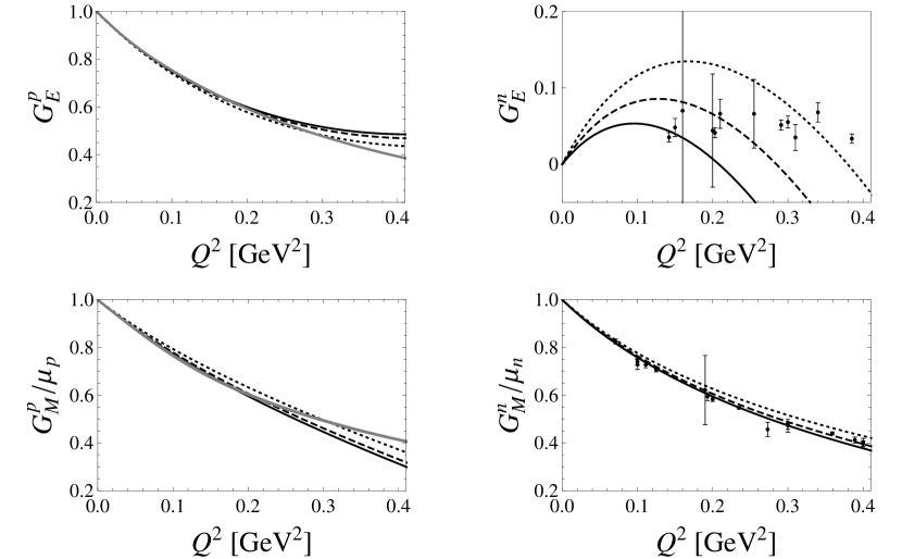
Figure 2: Sachs form factors of the nucleon at $\mathcal{O}(q^{3})$ including $\rho$, $\omega$, and $\Delta$, fitted to different ranges of momentum transfer $Q^{2}$. Full lines correspond to a fit up to $Q^{2}_{\textrm{max}}=0.2$ $\textrm{GeV}^{2}$, dashed lines up to $Q^{2}_{\textrm{max}}=0.3$ $\textrm{GeV}^{2}$, and dotted lines up to $Q^{2}_{\textrm{max}}=0.4$ $\textrm{GeV}^{2}$, respectively. The grey bands represent empirical fits of the form factors to the measured cross sections.

Using the LECs represented in Tables 1 and 3, the final results for the Sachs form factors are displayed in Fig. 2. Since our proton results are fitted directly to cross sections we show a grey band corresponding to a direct least-squares model fit for $G_{E}^{p}$ and $G_{M}^{p}$ to the measured cross sections and thus representing the experimental data Bernauer:2010wm . For the neutron form factors our results are plotted together with the respective set of data to which they have been fitted to. All curves describe the corresponding experimental data reasonably well for all four form factors. As indicated by the values of $\chi_{\textrm{red}}^{2}$ in Table 3, the description of the form factors adjusted to a wider range of momentum transfer worsens. While $G^{p}_{E}$ and $G^{n}_{M}$ are still in good agreement with the corresponding data for $Q^{2}_{\textrm{max}}=0.4$ $\textrm{GeV}^{2}$ (dotted curves), $G^{p}_{M}$ does not show sufficient curvature. The electric form factor of the neutron, $G^{n}_{E}$, cannot be described well beyond $Q^{2}\approx 0.3$ $\textrm{GeV}^{2}$. In all cases, the slope of $G^{n}_{E}$ at small values of the momentum transfer turns out too big.

In order to investigate the total results for the Sachs form factors in more detail, Fig. 3 shows the individual contributions of the different diagram sets for the fit up to $Q^{2}_{\textrm{max}}=0.4$ GeV². The dotted lines represent the diagrams involving $\pi\Delta$ loops which seem to adulterate the results for $Q^{2}\gtrsim 0.3$ GeV². Similarly to the short-dashed lines involving $\pi N$ loops only, the $\Delta$ contributions do not produce significant curvature. At larger values of $Q^{2}$, the strong linear $Q^{2}$ dependence of the dotted lines, especially for $G_{E}^{p}$, $G_{E}^{n}$, and $G_{M}^{p}$, together with their lack of curvature at $\mathcal{O}(q^{3})$ cannot be compensated by the strongly curved tree contributions of the vector mesons (long-dashed lines). For this reason, the quantitative description of the data worsens for larger values of $Q^{2}$ at the considered chiral order if the $\Delta$ is included explicitly. In agreement with Ref. Schindler:2005ke , the numerical contributions resulting from the vector-meson loop diagrams, denoted by the dash-dotted lines, turn out to be small.

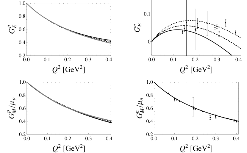
Figure 4: Sachs form factors of the nucleon at $\mathcal{O}(q^{3})$ including $\rho$ and $\omega$ fitted to different ranges of momentum transfer $Q^{2}$. Full lines correspond to a fit up to $Q^{2}_{\textrm{max}}=0.2$ $\textrm{GeV}^{2}$, dashed lines up to $Q^{2}_{\textrm{max}}=0.3$ $\textrm{GeV}^{2}$, and dotted lines up to $Q^{2}_{\textrm{max}}=0.4$ $\textrm{GeV}^{2}$, respectively. The grey bands represent empirical fits of the form factors to the measured cross sections.

Figure 4 displays the electromagnetic Sachs form factors without explicit $\Delta$ resonance (see Table 3). As opposed to Fig. 2, all fits describe the related data remarkably well for all four Sachs form factors. Consequently, the consistent inclusion of $\rho$ and $\omega$ mesons provides a satisfactory description of the electromagnetic form factors in the momentum transfer region $0\leq Q^{2}\leq 0.4$ $\textrm{GeV}^{2}$ already at third chiral order. In our calculation, the additional inclusion of the $\phi$ meson results in only a small numerical adjustment of the parameters in Table 3 and does not generate a visible improvement of the form factor curves.

In Ref. Schindler:2005ke , the electromagnetic form factors of the nucleon were calculated in Lorentz-invariant ChPT using the EOMS renormalization scheme up to and including $\mathcal{O}(q^{4})$. The vector mesons $\rho$, $\omega$, and $\phi$ were incorporated explicitly using parameterization II of Ref. Ecker:1989yg . The self-consistency relations for the $\rho$ meson couplings, as discussed in Sec. III B, were not considered in the effective Lagrangian. In order to discuss to what extent the self-consistent inclusion of vector mesons influences the description of the form factors, in Fig. 5 we display a comparison of our calculation, including explicit vector mesons only, and that of Ref. Schindler:2005ke . Even though our calculation involves one vector-meson degree of freedom less, namely the $\phi$ meson, and is only up to $\mathcal{O}(q^{3})$, the results for all Sachs form factors are slightly closer to experimental data for $Q^{2}\gtrsim 0.2$ $\textrm{GeV}^{2}$. In particular, our curve for the electric neutron form factor shows a better trend for larger values of the momentum transfer. The improved description can be explained by the following two reasons. On the one hand, the consistency relations lead to a parameterization which features the $\rho\gamma$ and $\rho\pi\pi$ couplings at leading order in distinction to the parameterization used in Ref. Schindler:2005ke featuring such couplings only at next-to-leading order. The re-ordering of terms changes the results favorably for larger values of $Q^{2}$. On the other hand, we fit our free coupling constants to the global trend of the form factor curves instead of adjusting them to the electric and magnetic radii and taking the remaining ones from results based on dispersion relations. This approach allows for a better overall descriptions of the form factor curves.

IV.4 Estimate of higher-order effects

In order to estimate the uncertainties originating in the truncation of the expansion at ${\cal O}(q^{3})$, we add polynomials in $Q^{2}$ to the Sachs form factors. The explicit form of the corresponding polynomial is motivated by an analysis of the maximal powers of $Q^{2}$ in the isoscalar and isovector Dirac and Pauli form factors, taking into account the available chiral structures at ${\mathcal{O}}(q^{3})$ with adjustable LECs. We find that the neglected structures which would appear in an ${\mathcal{O}}(q^{4})$ calculation can be parameterized as

$$\Delta G_{E}^{N} =\left(a_{N}\,Q^{2}-b_{N}\frac{Q^{2}}{4m_{p}^{2}}\right)Q^{2}, \Delta G_{M}^{N} =\left(a_{N}\,Q^{2}+b_{N}\right)Q^{2},$$ (32)

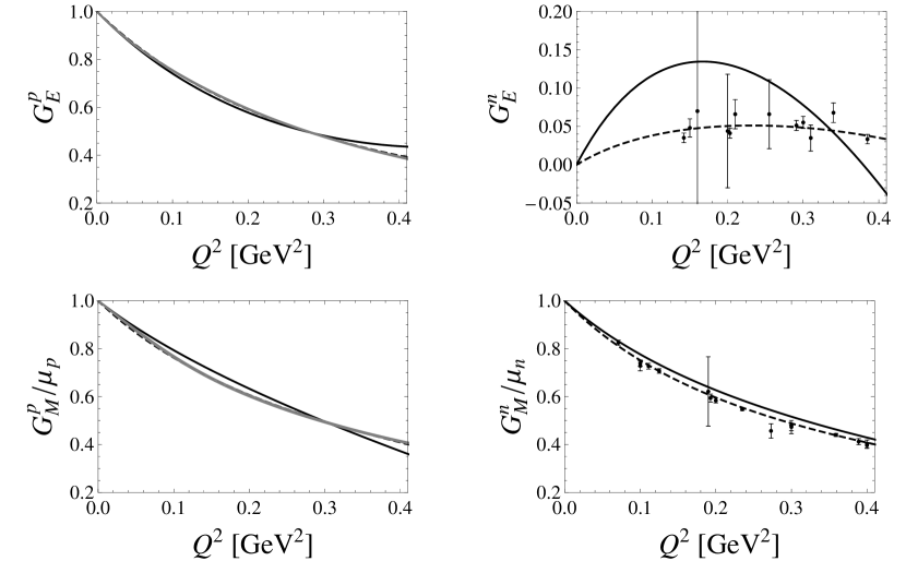
Figure 6: Sachs form factors including vector mesons and the $\Delta$ resonance. The full lines refer to the $\mathcal{O}(q^{3})$ results, whereas the dashed lines are supplemented by additional higher-order terms according to Eq. (32). The grey bands represent empirical fits of the form factors to the measured cross sections.

where $a_{N}$ and $b_{N}$ ($N=p,n$) denote unknown coefficients. The corrections to the electric Sachs form factors are purely of order $(Q^{2})^{2}$ while those to the magnetic Sachs form factors already start at order $Q^{2}$. To investigate the influence of these higher-order contributions we add them to the original expressions at ${\cal O}(q^{3})$ and perform a new simultaneous fit of all four ”improved” Sachs form factors to the data. The results of this procedure are shown in Fig. 6. Clearly, the inclusion of higher-order terms according to Eq. (32) changes the slopes of the Sachs form factors. The reason for this can be understood if one resolves the physical Sachs form factors into their respective isoscalar and isovector parts. Figure 7 indicates that an ${\mathcal{O}}(q^{3})$ calculation does not generate enough curvature for both, the electric and magnetic, isoscalar form factors. To fit to the data over a wider range of momentum transfer in terms of minimizing the total $\chi_{\text{red}}^{2}$ function, the respective slopes counterbalance the missing curvature. This overcompensation leads to a lower value for $\langle\left(r_{M}^{p}\right)^{2}\rangle$ and $\langle\left(r_{M}^{n}\right)^{2}\rangle$, as well as to a higher value for $|\langle\left(r_{E}^{n}\right)^{2}\rangle|$ than in the case with additional higher-order terms. A comparison between the radii obtained within the two approaches is shown in Table 6.

$\quad\langle\left(r_{E}^{p}\right)^{2}\rangle$	$\langle\left(r_{E}^{n}\right)^{2}\rangle$	$\langle\left(r_{M}^{p}\right)^{2}\rangle$	$\langle\left(r_{M}^{n}\right)^{2}\rangle$
$0.761$	$-0.440$	$0.574$	$0.667$
$0.718$	$-0.142$	$0.708$	$0.758$

Table 6: Mean square charge and magnetic radii of the nucleon obtained from the form factor results including the $\Delta$ resonance. The first row corresponds to the ${\mathcal{O}}(q^{3})$ results, whereas the second row also includes additional higher-order terms according to Eq. (32). The mean square radii are given in units of fm².

IV.5 Pion mass dependence of the form factors

Nucleon electromagnetic form factors have been calculated in the framework of lattice QCD (for a recent overview, see Refs. Yamazaki:2009zq ; Hagler:2009ni ; Bratt:2010jn ; Collins:2011mk ; Lin:2011sa and references therein). Several collaborations have reached pion masses down to 270 MeV. Systematic extrapolations to the physical value of the pion mass and the $Q^{2}$ dependence are necessary to compare the lattice form factor results to experimental data. Given the manifest Lorentz covariance of our results, they may provide useful guidance for extrapolations of lattice simulations. In lattice calculations it is more convenient to work with isoscalar and isovector form factors. Simulations of the isoscalar form factors are numerically expensive since they involve the evaluation of disconnected quark loops. For the isovector form factors the disconnected quark loop contributions cancel.

In Fig. 8 we display the pion-mass dependence of the Sachs form factors in the isovector and isoscalar channels. The quantities are derived from the results including $\rho$ and $\omega$ mesons as explicit resonant degrees of freedom. We stress that, at the given order of our calculation, the vector meson masses are independent of the pion mass (see, e.g., Refs. Djukanovic:2009zn ; Feng:2010es ; Feng:2011zk for a discussion of the quark-mass dependence of the $\rho$-meson mass). Extrapolations of lattice data of $G_{E}^{(v)}$ have been performed in Refs. Lin:2010ne ; Syritsyn:2009mx . The results qualitatively agree with ours as the values of the form factor fall off more slowly with increasing pion mass. In Ref. Hagler:2011zz the isovector magnetic moment is extrapolated to small pion masses using results from heavy-baryon ChPT Hemmert:2002uh . The pion-mass dependence and the value in the chiral limit are in good agreement with our corresponding findings plotted in Fig. 9.

In the present paper we fit the unknown LECs to experimental data at the physical pion mass. Alternatively, they can be fitted to lattice simulation data at different values of the pion mass resulting in a complete theoretical prediction of the observables. Whether this is a useful approach largely depends upon the range of pion masses in which the low-energy EFT is still applicable. The region of applicability depends on the calculational scheme and has yet to be studied more thoroughly.

V Summary

We have calculated the electromagnetic form factors of the nucleon at $\mathcal{O}(q^{3})$ in manifestly Lorentz-invariant baryon chiral perturbation theory including $\rho$ and $\omega$ mesons as well as the $\Delta$ resonance. In terms of constraints and perturbative renormalizability, we have incorporated the resonant degrees of freedom self-consistently into the EFT. To generate a systematic power counting we have applied the extended on-mass-shell renormalization scheme. Two of the undetermined low-energy coupling constants have been adjusted to the anomalous magnetic moments while the remaining six LECs have been fitted simultaneously to the experimental data for different ranges of momentum transfer up to $Q^{2}=0.4$ GeV². We found that the results incorporating vector mesons agree well with experimental data in a momentum transfer region $0\leq Q^{2}\leq 0.4$ $\textrm{GeV}^{2}$ while those also including the $\Delta$ describe the form factors only up to $Q^{2}\approx 0.3$ $\textrm{GeV}^{2}$. For larger values of $Q^{2}$, notably $G^{n}_{E}$ and $G^{p}_{M}$ disagree with the data. This is because the $\pi\Delta$ loop contributions at $\mathcal{O}(q^{3})$ feature a strong linear $Q^{2}$ dependence without sufficient curvature. Our results including $\rho$ and $\omega$ mesons at third chiral order agree at least as well with experimental data as the previously performed calculations of Refs. Kubis:2000zd ; Fuchs:2003ir at $\mathcal{O}(q^{4})$. This improvement is a hint towards the importance of a proper consideration of self-consistency relations among the couplings of the effective Lagrangian. The resulting form of the vector-mesonic Lagrangian gives rise to vector-meson dominance at leading order and deviations thereof are pushed to higher orders.

Figure 3: Decomposition of the Sachs form factors of the nucleon at $\mathcal{O}(q^{3})$ including vector mesons and the $\Delta$ resonance. Full lines: total results; long-dashed lines: tree contribution; short-dashed lines: contribution of set 1; dash-dotted lines: contribution of set 2; dotted lines: contribution of set 3 of Fig. 1, respectively.

Figure 5: Sachs form factors including vector mesons. The full lines refer to the $\mathcal{O}(q^{3})$ results of this work including $\rho$ and $\omega$ mesons and the dashed lines to the $\mathcal{O}(q^{4})$ results of Ref. Schindler:2005ke including $\rho$, $\omega$, and $\phi$. The grey bands represent empirical fits of the form factors to the measured cross sections.

Figure 7: Isocalar and isovector Sachs form factors including vector mesons and the $\Delta$ resonance. The full lines refer to the $\mathcal{O}(q^{3})$ results, whereas the dashed lines are supplemented by additional higher-order terms according to Eq. (32).

Figure 8: Electric and magnetic Sachs form factors in the isovector and isoscalar channel including $\rho$ and $\omega$ for different values of the pion mass $M_{\pi}$. The full lines refer to $M_{\pi}=140$ MeV, the dashed lines to $M_{\pi}=200$ MeV, the dash-dotted lines to $M_{\pi}=300$ MeV, and the dotted lines to $M_{\pi}=400$ MeV, respectively.

Figure 9: Pion-mass dependence of the anomalous magnetic moment in the isovector and isoscalar channels and of the mean square isovector Dirac and Pauli radii; the vertical dashed line indicates the physical pion mass.

- (1) H. Gao, Int. J. Mod. Phys. E 12, 1 (2003) [Erratum-ibid. E 12, 567 (2003)].
- (2) C. F. Perdrisat, V. Punjabi, and M. Vanderhaeghen, Prog. Part. Nucl. Phys. 59, 694 (2007).
- (3) D. Drechsel and T. Walcher, Rev. Mod. Phys. 80, 731 (2008).
- (4) P. J. Mohr, B. N. Taylor, and D. B. Newell, arXiv:1203.5425 [physics.atom-ph].
- (5) J. Beringer et al. [Particle Data Group Collaboration], Phys. Rev. D 86, 010001 (2012).
- (6) J. C. Bernauer, Lect. Notes Phys. 745, 79 (2008).
- (7) J. C. Bernauer et al. [A1 Collaboration], Phys. Rev. Lett. 105, 242001 (2010).
- (8) S. Weinberg, Physica A 96, 327 (1979).
- (9) J. Gasser and H. Leutwyler, Annals Phys. 158, 142 (1984).
- (10) J. Gasser, M. E. Sainio, and A. Švarc, Nucl. Phys. B307, 779 (1988).
- (11) S. Scherer, Prog. Part. Nucl. Phys. 64, 1 (2010).
- (12) S. Scherer and M. R. Schindler, A Primer for Chiral Perturbation Theory, Lect. Notes Phys. 830, 1 (2012).
- (13) E. E. Jenkins and A. V. Manohar, Phys. Lett. B 255, 558 (1991).
- (14) V. Bernard et al., Nucl. Phys. B388, 315 (1992).
- (15) H. B. Tang, arXiv:hep-ph/9607436.
- (16) T. Becher and H. Leutwyler, Eur. Phys. J. C 9, 643 (1999).
- (17) J. Gegelia and G. Japaridze, Phys. Rev. D 60, 114038 (1999).
- (18) T. Fuchs et al., Phys. Rev. D 68, 056005 (2003).
- (19) H. W. Fearing et al., Phys. Rev. D 56, 1783 (1997).
- (20) T. R. Hemmert, B. R. Holstein, and J. Kambor, J. Phys. G 24, 1831 (1998).
- (21) V. Bernard et al., Nucl. Phys. A635, 121 (1998).
- (22) B. Kubis and U.-G. Meißner, Nucl. Phys. A679, 698 (2001).
- (23) T. Fuchs, J. Gegelia, and S. Scherer, J. Phys. G 30, 1407 (2004).
- (24) T. Ledwig et al., Phys. Rev. D 85, 034013 (2012).
- (25) M. R. Schindler, J. Gegelia, and S. Scherer, Eur. Phys. J. A 26, 1 (2005).
- (26) T. Fuchs et al., Phys. Lett. B 575, 11 (2003).
- (27) S. Weinberg, The Quantum Theory Of Fields. Vol. 1: Foundations (Cambridge University Press, Cambridge, England, 1995), Chap. 7.6.
- (28) D. Djukanovic, J. Gegelia, and S. Scherer, Int. J. Mod. Phys. A 25, 3603 (2010).
- (29) D. Djukanovic et al., Phys. Rev. Lett. 93, 122002 (2004).
- (30) See Chap. 12 of Ref. weinbergQTFI .
- (31) N. Wies, J. Gegelia, and S. Scherer, Phys. Rev. D 73, 094012 (2006).
- (32) C. Hacker et al., Phys. Rev. C 72, 055203 (2005).
- (33) F. J. Ernst, R. G. Sachs, and K. C. Wali, Phys. Rev. 119, 1105 (1960).
- (34) G. Colangelo, J. Gasser, and H. Leutwyler, Phys. Rev. Lett. 86, 5008 (2001).
- (35) G. Ecker and M. Mojžiš, Phys. Lett. B 365, 312 (1996).
- (36) S. Weinberg, Phys. Rev. 166, 1568 (1968).
- (37) G. Ecker et al., Phys. Lett. B 223, 425 (1989).
- (38) K. Kawarabayashi and M. Suzuki, Phys. Rev. Lett. 16, 255 (1966).
- (39) Riazuddin and Fayyazuddin, Phys. Rev. 147, 1071 (1966).
- (40) J. C. Bernauer, Measurement of the elastic electron-proton cross section and separation of the electric and magnetic form factor in the range from 0.004 to 1 . Ph.D. thesis, Johannes Gutenberg-Universität Mainz, 2010.
- (41) K. M. Hanson et al., Phys. Rev. D 8, 753 (1973).
- (42) C. E. Jones-Woodward et al., Phys. Rev. C 44, 571 (1991).
- (43) A. K. Thompson et al., Phys. Rev. Lett. 68, 2901 (1992).
- (44) P. Markowitz et al., Phys. Rev. C 48, 5 (1993).
- (45) H. Gao et al., Phys. Rev. C 50, 546 (1994).
- (46) H. Anklin et al., Phys. Lett. B 336, 313 (1994).
- (47) T. Eden et al., Phys. Rev. C 50, 1749 (1994).
- (48) E. E. W. Bruins et al., Phys. Rev. Lett. 75, 21 (1995).
- (49) H. Anklin et al., Phys. Lett. B 428, 248 (1998).
- (50) M. Ostrick et al., Phys. Rev. Lett. 83, 276 (1999).
- (51) I. Passchier et al., Phys. Rev. Lett. 82, 4988 (1999).
- (52) C. Herberg et al., Eur. Phys. J. A 5, 131 (1999).
- (53) J. Becker et al., Eur. Phys. J. A 6, 329 (1999).
- (54) W. Xu et al., Phys. Rev. Lett. 85, 2900 (2000).
- (55) G. Kubon et al., Phys. Lett. B 524, 26 (2002).
- (56) W. Xu et al. [Jefferson Lab E95-001 Collaboration], Phys. Rev. C 67, 012201 (2003).
- (57) D. I. Glazier et al., Eur. Phys. J. A 24, 101 (2005).
- (58) B. Anderson et al. [Jefferson Lab E95-001 Collaboration], Phys. Rev. C 75, 034003 (2007).
- (59) E. Geis et al. [BLAST Collaboration], Phys. Rev. Lett. 101, 042501 (2008).
- (60) M. A. B. Beg and A. Zepeda, Phys. Rev. D 6, 2912 (1972).
- (61) T. Yamazaki et al., Phys. Rev. D 79, 114505 (2009)
- (62) P. Hägler, Phys. Rept. 490, 49 (2010).
- (63) J. D. Bratt et al. [LHPC Collaboration], Phys. Rev. D 82, 094502 (2010).
- (64) S. Collins et al., Phys. Rev. D 84, 074507 (2011).
- (65) H.-W. Lin and S. D. Cohen, arXiv:1104.4319 [hep-lat].
- (66) D. Djukanovic et al., Phys. Lett. B 680, 235 (2009).
- (67) X. Feng, K. Jansen, and D. B. Renner, Phys. Rev. D 83, 094505 (2011).
- (68) X. Feng et al., Phys. Rev. Lett. 107, 081802 (2011).
- (69) M. F. Lin et al., PoS LAT2009, 127 (2009).
- (70) S. N. Syritsyn et al., Phys. Rev. D 81, 034507 (2010).
- (71) P. Hägler, Prog. Theor. Phys. Suppl. 187, 221 (2011).
- (72) T. R. Hemmert and W. Weise, Eur. Phys. J. A 15, 487 (2002).