Constraining clumpy dusty torus models
using optimized filter sets

Abstract

Recent success in explaining several properties of the dusty torus around the central engine of active galactic nuclei has been gathered with the assumption of clumpiness. The properties of such clumpy dusty tori can be inferred by analyzing spectral energy distributions (SEDs), sometimes with scarce sampling given that large aperture telescopes and long integration times are needed to get good spatial resolution and signal. We aim at using the information already present in the data and the assumption of clumpy dusty torus, in particular, the CLUMPY models of Nenkova et al., to evaluate the optimum next observation such that we maximize the constraining power of the new observed photometric point. To this end, we use the existing and barely applied idea of Bayesian adaptive exploration, a mixture of Bayesian inference, prediction and decision theories. The result is that the new photometric filter to use is the one that maximizes the expected utility, which we approximate with the entropy of the predictive distribution. In other words, we have to sample where there is larger variability in the SEDs compatible with the data with what we know of the model parameters. We show that Bayesian adaptive exploration can be used to suggest new observations, and ultimately optimal filter sets, to better constrain the parameters of the clumpy dusty torus models. In general, we find that the region between 10 and 200 $\mu$m produces the largest increase in the expected utility, although sub-mm data from ALMA also prove to be useful. It is important to note that here we are not considering the angular resolution of the data, which is key when constraining torus parameters. Therefore, the expected utilities derived from this methodology must be weighted with the spatial resolution of the data.

1 Introduction

The unified model for active galaxies (Antonucci, 1993; Urry & Padovani, 1995) is based on the existence of a dusty toroidal structure surrounding the central region of active galactic nuclei (AGN). Considering this geometry of the obscuring material, the central engines of Type-1 AGN can be seen directly, resulting in typical spectra with both narrow and broad emission lines, whereas in Type-2 AGN the broad line region (BLR) is obscured.

The infrared (IR) range (and particularly the mid-infrared; MIR) is key to characterize the torus, since the dust reprocesses the optical and ultraviolet radiation generated in the accretion process and re-emits it in this range. However, considering the small torus size, high angular resolution turns to be essential to isolate as much as possible its emission.

Pioneering work in modelling the dusty torus (Pier & Krolik, 1992, 1993) assumed a uniform dust density distribution to simplify the modelling, although from the start, Krolik & Begelman (1988) realized that smooth dust distributions cannot survive within the immediate AGN vicinity. To solve the various discrepancies between observations and models, an intensive search for an alternative torus geometry has been carried out in the last decade. The clumpy torus models (Nenkova et al., 2002, 2008a, 2008b; Hönig et al., 2006; Schartmann et al., 2008) propose that the dust is distributed in clumps, instead of homogeneously filling the torus volume. These models are making significant progress in accounting for the MIR emission of AGN (Mason et al., 2006, 2009; Mor et al., 2009; Horst et al., 2008, 2009; Nikutta et al., 2009; Ramos Almeida et al., 2009, 2011a, 2011b; Hönig et al., 2010; Alonso-Herrero et al., 2011, 2012a, 2012b).

In previous works we constructed subarcsecond resolution IR spectral energy distributions (SEDs) for about 20 nearby Seyfert galaxies and successfully reproduced them with the clumpy torus models of Nenkova et al. (hereafter CLUMPY). It is worth mentioning, however, that some observational results show that the CLUMPY models alone cannot explain the IR SEDs of a sample of PG quasars (Mor et al., 2009; Mor & Netzer, 2012). The latter authors needed an additional hot dust component to reproduce the SEDs. Moreover, recent interferometry results (Kishimoto et al., 2011; Hönig et al., 2012) indicate that a single component torus does not reproduce the observations.

The CLUMPY database now contains $\sim$5$\times$10⁶ models, calculated for a fine grid of model parameters. The inherent degeneracy between these parameters has to be taken into account when fitting the observables. To this end, we developed the Bayesian inference tool BayesClumpy. Details on the interpolation methods and algorithms employed can be found in Asensio Ramos & Ramos Almeida (2009). We point out that, given the specificities of the Bayesian inference approach we follow, in the following analysis we will not be using the original set of models described in Nenkova et al. (2008a, b), but an interpolated version of them.

In Ramos Almeida et al. (2009, 2011b) we fitted IR SEDs constructed using MIR nuclear fluxes obtained with 8 m telescopes and NIR measurements of similar resolution from the literature (see also Alonso-Herrero et al. 2011). Some of the SEDs were well-sampled (e.g. the Circinus galaxy and Centaurus A) whilst others comprised just three photometric data points (e.g. NGC 1365 and NGC 1386). The better the sampling of the SED, the more constrained the torus parameters (see e.g. Alonso-Herrero et al. 2012a). Considering the need for 8-10 m telescopes to isolate the torus emission, it is necessary to determine the minimum number of filters required to constrain the model parameters. We utilize the output of our code BayesClumpy in a Bayesian experiment design framework. Our aim is to design the experiment (observation of a source using a selected filter) that introduces more constraints for the parameters of the CLUMPY models. Using our Bayesian approach, we can investigate which and how many optical, IR, and sub-mm filters restrict the most the parameter space, as well as which wavelengths provide more information about each of the parameters. Although here we present results for the models of Nenkova et al., the formalism can be applied to any other set of models, including multi-component ones. Thus, this work can be useful for the community when applying for telescope observations.

2 Clumpy Dusty Torus Models and Bayesian approach

The CLUMPY models of Nenkova et al. (2002) hold that the dust surrounding the central engine of an AGN is distributed in clumps. These clumps are distributed with a radial extent $Y=R_{o}/R_{d}$, where $R_{o}$ and $R_{d}$ are the outer and inner radius of the toroidal distribution, respectively (see Figure 1). The inner radius is defined by the dust sublimation temperature ($T_{sub}\approx 1500$ K), with $R_{d}=0.4~{}(1500~{}K~{}T_{sub}^{-1})^{2.6}(L/10^{45}\,\mathrm{erg~{}s^{-1}})^{0.5}$ pc. Within this geometry, each clump has the same optical depth ($\tau_{V}$). The average number of clouds along a radial equatorial ray is $N_{0}$. The radial density profile is a power-law ($\propto r^{-q}$). A width parameter, $\sigma$, characterizes the angular distribution of the clouds, which has a smooth edge. The number of clouds along the LOS at an inclination angle $i$ is $N_{LOS}(i)=N_{0}~{}e^{(-(i-90)^{2}/\sigma^{2})}$. For a detailed description of the clumpy models see Nenkova et al. (2002, 2008a, 2008b).

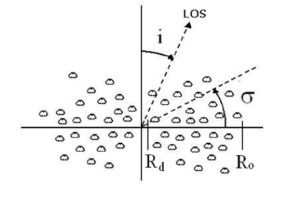
Figure 1: Scheme of the clumpy torus described in Nenkova et al. (2008a, b). The radial extent of the torus is defined by the outer radius ($R_{o}$) and the dust sublimation radius ($R_{d}$). All the clouds are supposed to have the same $\tau_{V}$, and $\sigma$ characterizes the width of the angular distribution. The number of cloud encounters is function of the viewing angle, $i$.

In every Bayesian scheme, one needs to specify a-priori information about the model parameters. This is done through the prior distribution (see Asensio Ramos & Ramos Almeida, 2009, for more details). We consider them to be truncated uniform distributions for the six model parameters in the intervals reported in Table 1. Therefore, we give the same weight to all the values in each interval. To compare with the observations, BayesClumpy simulates the effect of the employed filters on the SED by integrating the product of the synthetic SED and the filter transmission curve. Observational errors are assumed to be Gaussian.

Table 1: Clumpy Model Parameters and Considered Intervals

Parameter	Abbreviation	Interval
Width of the angular
distribution of clouds	$\sigma$	[15°, 75°]
Radial extent of the torus	$Y$	[5, 100]
Number of clouds along
the radial equatorial direction	$N_{0}$	[1, 15]
Power-law index of the
radial density profile	$q$	[0, 3]
Inclination angle of the torus	$i$	[0°, 90°]
Optical depth per single cloud	$\tau_{V}$	[5, 150]

The results of the fitting process of the IR SEDs with the CLUMPY models are the posterior distributions for the six free parameters that describe the models. When the observed data introduce sufficient information into the fit, the resulting probability distributions will clearly differ from the input uniform distributions, either showing trends or being centered at certain values within the intervals considered.

3 Bayesian adaptive exploration

In this section we briefly describe our approach to the experiment design, following the lines of the theory of Bayesian adaptive exploration, as developed by Sebastiani & Wynn (2000) and Loredo (2004). The output of this analysis is a measure of the “utility” of each one of the available photometric filters to constrain the models introduced in Sec. 2.

3.1 General problem

The problem at hand can be stated as follows. Let $\mathbf{D}$ be an $N$-dimensional vector containing observations that sample an AGN SED using $N$ different filters. A fundamental assumption that we have to make (inherent to any inference process) is to consider that the SEDs we are analyzing can be correctly reproduced with the CLUMPY models. If we have a set of $M$ new filters available (in our case, from the list of Table 2) to carry out new observations, we want to know which is the filter that, when we acquire a new observation with it, maximizes the amount of information that we gain about the model parameters. As stated before, this is a crucial problem to be solved when applying for observing time in large-aperture telescopes, given the large overpetition of such telescopes. In order to solve this problem, we apply a recent methodology of Bayesian experiment design termed Bayesian adaptive exploration (BAE), as presented by Sebastiani & Wynn (2000) and Loredo (2004). In essence, BAE can be understood as an iteration of an observation-inference-design scheme. Starting from the current observations, we infer the model parameters using standard Bayesian techniques like what can be achieved with BayesClumpy (Asensio Ramos & Ramos Almeida, 2009). The inference process allows us to predict new data at the light of the information gained from the observations. From these synthetic observations, it is possible to predict which new experiments will carry more information. The decision of which is the best experiment to carry out is not an issue of Bayesian inference, but one has to rely on the foundations of Bayesian decision theory (Berger, 1985). This procedure can be iterated until convergence, although we will not pursue this issue here, only the suggestion of a new observations. We summarize in the following the tools that we have used in this paper.

Table 2: Filters considered in this work

ID	Instrument	Telescope	$\lambda_{0}$ [$\mu$m]	FWHM [$\mu$m]
F606W	WFPC2	HST	0.603	0.22
F791W	WFPC2	HST	0.806	0.19
F110W	NICMOS	HST	1.102	0.59
F160W	NICMOS	HST	1.595	0.40
F187N	NICMOS	HST	1.874	0.02
F222M	NICMOS	HST	2.216	0.14
J	NACO	VLT	1.265	0.25
H	NACO	VLT	1.659	0.34
Ks	NACO	VLT	2.180	0.35
IB2.42	NACO	VLT	2.431	0.06
L’	NACO	VLT	3.805	0.63
IB4.05	NACO	VLT	4.056	0.06
M’	NACO	VLT	4.781	0.60
Js	ISAAC	VLT	1.249	0.16
H	ISAAC	VLT	1.652	0.30
Ks	ISAAC	VLT	2.164	0.27
L	ISAAC	VLT	3.779	0.58
Nb_M	ISAAC	VLT	4.657	0.10
Js	SOFI	NTT	1.249	0.16
H	SOFI	NTT	1.652	0.30
Ks	SOFI	NTT	2.164	0.27
J	IRCAM3	UKIRT	1.248	0.16
H	IRCAM3	UKIRT	1.630	0.30
K	IRCAM3	UKIRT	2.200	0.34
L’	IRCAM3	UKIRT	3.774	0.70
M	IRCAM3	UKIRT	4.758	0.64
H	IRAC-1	2.2m ESO	1.651	0.30
K	IRAC-1	2.2m ESO	2.161	0.27
K’	NSFCam	IRTF	2.113	0.34
L	NSFCam	IRTF	3.498	0.61
K	TIMMI2	3.6m ESO	2.161	0.27
L	TIMMI2	3.6m ESO	3.498	0.58
M	TIMMI2	3.6m ESO	4.758	0.64
Si2	MICHELLE	Gemini N	9.150	0.87
N	MICHELLE	Gemini N	10.50	5.58
Si4	MICHELLE	Gemini N	10.54	1.01
N’	MICHELLE	Gemini N	11.30	2.40
Si6	MICHELLE	Gemini N	12.72	1.16
Qa	MICHELLE	Gemini N	18.47	1.95
Q	MICHELLE	Gemini N	20.86	8.97
Si2	T-ReCS	Gemini S	8.725	0.78
N	T-ReCS	Gemini S	10.31	5.24
Np	T-ReCS	Gemini S	11.35	2.27
Si5	T-ReCS	Gemini S	11.65	1.16
Qa	T-ReCS	Gemini S	18.34	1.52
N	OSCIR	CTIO	10.82	5.16
IHW18	OSCIR	CTIO	18.12	1.61
ArIII	VISIR	VLT	8.996	0.13
SIV	VISIR	VLT	10.46	0.16
PAH2	VISIR	VLT	11.27	0.59
PAH2_2	VISIR	VLT	11.74	0.37
NeII_1	VISIR	VLT	12.27	0.19
NeII_2	VISIR	VLT	13.04	0.22
Q2	VISIR	VLT	18.75	0.86
CC_Si2	CanariCam	GTC	8.67	1.04
CC_N	CanariCam	GTC	10.31	5.25
CC_Q4	CanariCam	GTC	20.39	0.97
CC_Q8	CanariCam	GTC	24.53	0.75
LWC-31.5	FORCAST	SOFIA	31.38	4.54
LWC-33.6	FORCAST	SOFIA	33.60	1.56
LWC-34.8	FORCAST	SOFIA	34.81	3.42
LWC-37.1	FORCAST	SOFIA	37.18	2.13
PACS70	PACS	Herschel	71.07	20.9
PACS100	PACS	Herschel	102.2	36.0
PACS160	PACS	Herschel	165.9	74.5
SPIRE250	SPIRE	Herschel	251.6	77.9
SPIRE350	SPIRE	Herschel	353.3	106.6
SPIRE500	SPIRE	Herschel	508.8	198.2
ALMA Ch9	…	ALMA	460.0	77.3
ALMA Ch7	…	ALMA	945.0	280.2

Let $\theta$ be the vector with the parameters that define the CLUMPY model. Once the set of observations $\mathbf{D}$ for the current filters have been acquired, the role of Bayesian inference is to compute the posterior distribution $p(\mbox{\boldmath$\theta$}|\mathbf{D},I)$ that encodes all the information we possess about the model parameters at the light of the observations and assuming our current experiment $I$. Using the posterior distribution, it is possible to predict which is the expected value of a fictitiuos new observation $o$ at filter $f$ under the experiment $I_{f}$ using the well-known predictive distribution (e.g., Bishop, 2006):

$$p(o|\mathbf{D},I_{f}) = \int d\mbox{\boldmath$\theta$}\,p(o,\mbox{\boldmath$\theta$}|\mathbf{D},I_{f})$$ (1)

$$= \int d\mbox{\boldmath$\theta$}\,p(o|\mbox{\boldmath$\theta$},\mathbf{D},I_{f})\,p(\mbox{\boldmath$\theta$}|\mathbf{D},I_{f}),$$

where the conditioning on $\mathbf{D}$ of $p(o|\mbox{\boldmath$\theta$},\mathbf{D},I_{f})$ is, in fact, irrelevant once $\theta$ is known. The term $p(o|\mbox{\boldmath$\theta$},\mathbf{D},I_{f})$ is just the likelihood of getting the new observation $o$. According to the Bayesian decision theory, one should choose the filter $f$ that maximizes the expected utility (EU), defined as:

$$EU(f)=\int do\,p(o|\mathbf{D},I_{f})\,U(o,f),$$ (2)

where the function $U(o,f)$ is the utility, a function that is at the core of decision theory and that quantifies the information gain of a new experiment and can also include the potential cost of the new experiment at filter $f$ (i.e., we could potentially include factors that, e.g., increase the weight of filters that provide a better spatial resolution or that takes into account the difficulty of being awarded with observing with a certain telescope). In other words, we have to choose the filter that maximizes the value of the expected utility using the predictions of the flux at filter $f$ according to our current knowledge of the model.

Table 3: Measured flux densities

Filters	NGC 1566	NGC 4151	Circinus	NGC 1068	avg Sy1	avg Sy2
NICMOS F110W	$-$	60$\pm$6	$-$	9.8$\pm$2	$-$	$-$
NICMOS F160W	$-$	100$\pm$10	1.6$\pm$0.2	98$\pm$15	0.05$\pm$0.01	0.001$\pm$0.001
NICMOS F222M	$-$	197$\pm$20	$-$	445$\pm$100	$-$	$-$
NACO J	1.1$\pm$0.1	$-$	4.8$\pm$0.7	$-$	0.07$\pm$0.03	0.003$\pm$0.002
NACO Ks	2.1$\pm$0.1	$-$	19$\pm$2	$-$	0.12$\pm$0.05	0.023$\pm$0.018
NACO 2.42		$-$	31$\pm$3	$-$	$-$	$-$
NACO L’	7.8$\pm$0.1	$-$	380$\pm$38	$-$	0.35$\pm$0.11	0.15$\pm$0.09
NACO M’		$-$	1900$\pm$190	$-$	0.48$\pm$0.13	0.31$\pm$0.09
NSFCam L	$-$	325$\pm$65	$-$	$-$	$-$	$-$
IRCAM3 M	$-$	449$\pm$34	$-$	2270$\pm$341	$-$	$-$
TIMMI2 L	$-$	$-$	$-$	920$\pm$138	$-$	$-$
OSCIR N	$-$	1320$\pm$200	$-$	$-$	$-$	$-$
OSCIR IHW18	$-$	3200$\pm$800	$-$	$-$	$-$	$-$
T-ReCS Si2	29$\pm$4	$-$	5620$\pm$843	10000$\pm$1500	1.00$\pm$0.15	1.00$\pm$0.15
T-ReCS Qa	63$\pm$9	$-$	12791$\pm$3198	21773$\pm$5443	4.46$\pm$2.19	4.36$\pm$1.93
VISIR PAH2_2	117$\pm$29	$-$	$-$	$-$	$-$	$-$
VISIR Q2	128$\pm$32	$-$	$-$	$-$	$-$	$-$

Fluxes in mJy from Ramos Almeida et al. (2009, 2011b) and Alonso-Herrero et al. (2011). In the case of the Sy1 and Sy2 templates, the fluxes have been normalized to the central wavelength of the T-ReCS Si2 filter.

The previous definitions are somewhat obvious and the core of Bayesian decision theory is located on the appropriate definition of the utility function. We follow here the suggestion of Lindley (1956) (see also Loredo, 2004), who suggested that, since we want to maximize the information about the model parameters $\theta$, it makes sense to use the information encoded on the posterior for $\theta$, as measured by the negative differential entropy:

$$U(o,f)=-H[\mbox{\boldmath$\theta$}|o,\mathbf{D},I_{f}],$$ (3)

where the notation means that the entropy is computed for the posterior for the distribution $p(\mbox{\boldmath$\theta$}|o,\mathbf{D},I_{f})$. The differential entropy is, following the standard definition, given by:

$$H[\mbox{\boldmath$\theta$}|o,\mathbf{D},I_{f}]=-\int d\mbox{\boldmath$\theta$}\,p(\mbox{\boldmath$\theta$}|o,\mathbf{D},I_{f})\log p(\mbox{\boldmath$\theta$}|o,\mathbf{D},I_{f}).$$ (4)

Consequently, we have to compute the following quantity for all the available filters

$$\mathrm{EU}(f)=\int\int do\,d\mbox{\boldmath$\theta$}\,p(o|\mathbf{D},I_{f})\,p(\mbox{\boldmath$\theta$}|o,\mathbf{D},I_{f})\log p(\mbox{\boldmath$\theta$}|o,\mathbf{D},I_{f}),$$ (5)

and choose the filter $f$ that maximizes it. One could plug the expression for the predictive distribution of Eq. (1) on the expected utility and end up with a triple multidimensional integral that needs to be computed for each value of $f$. However, it turns out to be much easier to plug Eqs. (3) and (4) onto Eq. (2) and apply Bayes theorem (e.g., Gregory, 2005) to $\log p(\mbox{\boldmath$\theta$}|o,\mathbf{D},I_{f})$, so that we have to end up with:

$$\mathrm{EU}(f) = \int do\,d\mbox{\boldmath$\theta$}\,p(\mbox{\boldmath$\theta$}|\mathbf{D},I_{f})\,p(o|\mbox{\boldmath$\theta$},\mathbf{D},I_{f})\log p(o|\mbox{\boldmath$\theta$},\mathbf{D},I_{f})$$ (6)

$$+ \int do\,d\mbox{\boldmath$\theta$}\,p(o|\mbox{\boldmath$\theta$},\mathbf{D},I_{f})\,p(\mbox{\boldmath$\theta$}|\mathbf{D},I_{f})\log p(\mbox{\boldmath$\theta$}|\mathbf{D},I_{f})$$

$$- \int do\,d\mbox{\boldmath$\theta$}\,p(\mbox{\boldmath$\theta$}|\mathbf{D},I_{f})\,p(o|\mathbf{D},I_{f})\log p(o|\mathbf{D},I_{f}).$$

Using the definition of entropy of Eq. (4), we can rewrite the previous expression as:

$$\mathrm{EU}(f) = -\int d\mbox{\boldmath$\theta$}\,p(\mbox{\boldmath$\theta$}|\mathbf{D},I_{f})H[o|\mbox{\boldmath$\theta$},\mathbf{D},I_{f}]$$ (7)

$$- \int do\,p(o|\mbox{\boldmath$\theta$},\mathbf{D},I_{f})H[\mbox{\boldmath$\theta$}|\mathbf{D},I_{f}]$$

$$+ \int d\mbox{\boldmath$\theta$}\,p(\mbox{\boldmath$\theta$}|\mathbf{D},I_{f})H[o|\mathbf{D},I_{f}].$$

Note that the entropies $H[\mbox{\boldmath$\theta$}|\mathbf{D},I_{f}]$ and $H[o|\mathbf{D},I_{f}]$ can be extracted from the integrals because they do not depend on the integration variable. Given that the probability distributions are normalized to unit area, the expression simplifies to:

$$\mathrm{EU}(f) = -\int d\mbox{\boldmath$\theta$}p(\mbox{\boldmath$\theta$}|\mathbf{D},I_{f})H[o|\mbox{\boldmath$\theta$},\mathbf{D},I_{f}]$$ (8)

$$- H[\mbox{\boldmath$\theta$}|\mathbf{D},I_{f}]+H[o|\mathbf{D},I_{f}].$$

3.2 Simplifications

Clearly, the second term (the entropy of the posterior distribution considering the existing data) is independent of the election of the new filter, so it becomes constant with respect to $f$ and can be dropped from the computation. The term $H[o|\mbox{\boldmath$\theta$},\mathbf{D},I_{f}]$, which is the entropy of the likelihood for the new observed point at filter $f$, can be assumed to be constant if the expected noise is independent of the measurement. This is the case when the measurement for the new filter $f$ is done under the presence of additive (Gaussian) noise with a variance that is independent of $f$. However, this is not usually the case since the noise variance at different wavelengths can vary a lot. Assuming that the observation $o$ is perturbed with Gaussian noise with variance $\sigma_{f}$, the likelihood $p(o|\mbox{\boldmath$\theta$},\mathbf{D},I_{f})$ is a Gaussian distribution, so its entropy is analytically expressed as:

$$H[o|\mbox{\boldmath$\theta$},\mathbf{D},I_{f}]=\frac{1}{2}\log\left(2\pi\mathrm{e}\sigma_{f}^{2}\right).$$ (9)

Given that the previous entropy is independent of $\theta$, it can be extracted from the integral in Eq. (8) and use the fact that the posterior is normalized to unit area. Therefore, the final expression for the expected utility that we use in this work simplifies to:

$$\mathrm{EU}(f)=-\frac{1}{2}\log\left(2\pi\mathrm{e}\sigma_{f}^{2}\right)-\int do\,p(o|\mathbf{D},I_{f})\log p(o|\mathbf{D},I_{f}),$$ (10)

with $p(o|\mathbf{D},I_{f})$ given by Eq. (1). Note that if the noise variance does not depend on $f$, we end up with the expected utility derived by Sebastiani & Wynn (2000) and Loredo (2004). They noted that the previous expression leads to a maximum entropy sampling, so that we select the new filter where we know the least. In other words, we should sample where the current values of the model parameters allow for a large variability of the SED.

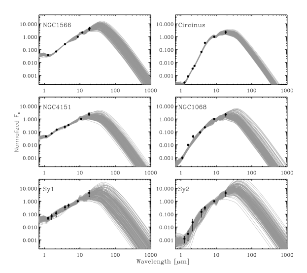
Figure 2: IR SEDs used in this paper. The circles with the error bars are the observed points and they are drawn at the central wavelength of each filter. The left panels correspond to Sy1 galaxies, while the right panels are Sy2. The average Sy1 and Sy2 SEDs have been obtained by a simple mean of galaxies belonging to each group once their SEDs have been interpolated onto the filters in which Circinus was observed (REF). Fluxes are normalized to the data point closer to 10 $\mu$m. The grey curves are the CLUMPY SEDs that have been sampled from the posterior.

3.3 Technicalities

The computation of the integral of Eq. (10) can be done following Loredo (2004), who used a Monte Carlo estimation technique. First, we can compute a Monte Carlo estimation of $p(o|\mathbf{D},I_{f})$ using:

$$p(o|\mathbf{D},I_{f})\approx\frac{1}{N_{\mathrm{pos}}}\sum_{j=1}^{N_{\mathrm{pos}}}p(o|\mbox{\boldmath$\theta$}_{j},\mathbf{D},I_{f}),$$ (11)

where the $\mbox{\boldmath$\theta$}_{j}$ are $N_{\mathrm{pos}}$ samples from the posterior distribution $p(\mbox{\boldmath$\theta$}|\mathbf{D},I_{f})$ that have been previously computed with BayesClumpy for the current set of observations. Then, the integral of Eq. (10), the entropy of the predictive distribution, is computed using another Monte Carlo estimation:

$$H[o|\mathbf{D},I_{f}]\approx\frac{1}{N_{\mathrm{pred}}}\sum_{j=1}^{N_{\mathrm{pred}}}\log p(o_{j}|\mathbf{D},I_{f}),$$ (12)

where the $o_{j}$ are samples from $p(o|\mathbf{D},I_{f})$. However, we have tested that better results are obtained if a simple trapezoidal quadrature is used to compute the integral of Eq. (10). To this end, we discretize the posible range of variation of $o$ in bins. For each bin, we compute $p(o|\mathbf{D},I_{f})$ using the Monte Carlo estimation of Eq. (11). At the end, we compute the entropy of the predictive distribution as:

$$H[o|\mathbf{D},I_{f}]\approx\sum_{j}w_{j}p(o_{j}|\mathbf{D},I_{f})\log p(o_{j}|\mathbf{D},I_{f}),$$ (13)

with $w_{j}$ the standard trapezoidal weights (e.g., Press et al., 1986).

4 Results

The Bayesian Adaptive Exploration theory, as summarized in the previous section, is applied to the case of SEDs generated by the emission of a clumpy torus around an AGN. Under the assumption that the parametric models of Nenkova et al. (2008a, b) are representative of the underlying physics, our analysis allows us to search for the filter that introduces more restrictions on the model parameters.

Our set of potential filters is listed in Table 2. Our aim is to consider a sufficiently complete list of photometric filters available in many medium- to large-aperture telescopes. In particular, we are considering all the optical, NIR, MIR and far-IR (FIR) filters that we have employed in our previous work, plus four new MIR filters from the CanariCam instrument, which has recently started to operate at the 10 m Gran Telescopio Canarias (GTC), and another four filters from the Long Wavelength Camera (LWC) on the FORCAST instrument. FORCAST is a MIR/FIR camera for the Stratospheric Observatory For Infrared Astronomy (SOFIA; Young et al. 2012). Finally, to inspect whether or not sub-mm data can set any constraints on the model parameters, we have also added channels 7 and 9 of ALMA, although they cannot be considered filters per se. They are simulated as a square transmission efficiency with a peak of 80% in the ranges $[800,1090]$ $\mu$m for channel 7 and $[420,500]$ $\mu$m for channel 9. Table 2 presents the filter identification, together with the instrument and telescope in which they are mounted. Additionally, we have tabulated the central wavelength of the filter, computed as $\lambda_{0}=\int\lambda R(\lambda)d\lambda/\int R(\lambda)d\lambda$, where $R(\lambda)$ is the transmission efficiency of the filter, and the full-width at half maximum (FWHM). The transmission efficiency of the filters have been obtained from the literature.

It is important to note that, for the sake of simplicity, in this work we are not taking into account the angular resolution provided by the different instruments considered here. In other words, we are assuming that all instruments listed in Table 2 are equivalent except in the wavelength coverage. However, the reader must keep in mind that high spatial resolution is mandatory when trying to isolate the torus emission. Thus, aside from the expected utilities derived here for the different instruments, it is important to consider the resolution when deciding which should be the next observation.

Figure 3: Expected utility (EU) computed using Eq. (8) and normalized to the maximum of each panel. EU is calculated for all filters not present in the observations. The first column refers to the case in which we use all the available observations of the galaxy. The central and right columns refer to the cases in which we only keep observations below and above 4 $\mu$m, respectively. For an easier visualization, the different wavelength ranges have been color-coded.

Black dots correspond to filters with $\lambda_{0}\leq 6$ $\mu$m, red dots to $6<\lambda_{0}\leq 25$ $\mu$m, blue dots to $25<\lambda_{0}\leq 200$ $\mu$m and green dots to $\lambda_{0}>200$ $\mu$m.

To demonstrate our approach, we have used four SEDs, two representative of Seyfert 1 (Sy1) and another two representative of Seyfert 2 (Sy2) galaxies. These SEDs have been discussed by Ramos Almeida et al. (2009, 2011b) and Alonso-Herrero et al. (2011) using a deep Bayesian analysis. Additionally, here we use the Sy1 and Sy2 average templates presented in Ramos Almeida et al. (2011b). These mean templates were constructed using individual Sy1 and Sy2 SEDs of angular resolution $\la$0.55 arcsec, that were first interpolated onto the Circinus wavelength grid (1.265, 1.60, 2.18, 3.80, 4.80, 8.74, and 18.3 $\mu$m), and then normalized to the central wavelength of the T-ReCS Si2 filter (8.74 $\mu$m). These flux densities and their associated errors are shown in Table 3 and are displayed in graphical form in Fig. 2, normalized to the filter that is closer to 10 $\mu$m. Note that the SEDs that we have selected have quite dense samplings, as opposed to other sparsely sampled ones (Ramos Almeida et al., 2009, 2011b).

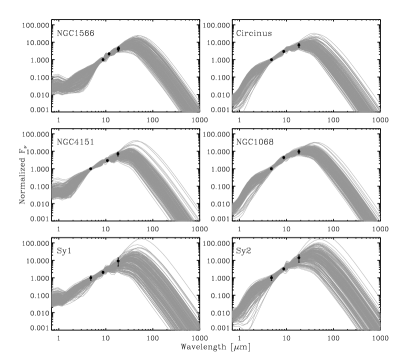
Figure 4: Same as in Fig. 2, but considering observed data point below and above 4 $\mu m$ from the complete SEDs (6 left and 6 right panels respectively).

For each SED we have carried out a full Bayesian analysis using BayesClumpy. This analysis relies on sampling the posterior distribution function as a function of the model parameters (shown in Table 1). We have used flat priors for all model parameters. For the Sy1 galaxies, we have additionally included an AGN spectrum, which is added to the CLUMPY SED. The shape of the AGN spectrum is the same that is considered for the infrared pumping of the dust in the torus (Nenkova et al., 2008a). Likewise, we also take into account a certain amount of extinction following the law of Chiar et al. (2000). This introduces the free parameter $A_{V}$, which is included into the inference for Sy1 galaxies with a flat prior in the range $[0,5]$ mag. The inclusion of these two ingredients turns out to be essential for obtaining reliable results for Sy1 sources.

BayesClumpy  generates samples of model parameters distributed according to the posterior distribution. Figure 2 shows, apart from the observed points, a representation of the SEDs reconstructed from the model parameters sampled from the posterior. Note that the sampled SEDs have a small variability close to the observed points with the smaller error bars. In principle, and according to the maximum entropy sampling derived by Sebastiani & Wynn (2000) and Loredo (2004), the filter that we should select has to be located close to the wavelength where the SEDs contain larger variability with the observational information we have acquired. An evaluation of Eq. (10), following the ideas of Sec. 3.3, gives the results displayed in the left column of Fig. 3. This figure represents the value of $\mathrm{EU}(f)$ for filter $f$ versus the central wavelength of the filter. The noise associated to any new observation, $\sigma_{f}$, depends on the wavelength: we consider 10% of the value of the flux at $\lambda\leq 5~{}\mu m$, 20% at $5~{}\mu m<\lambda<25~{}\mu m$ and 30% at $\lambda\geq 25~{}\mu m$. These are the typical uncertainties that we measured for individual galaxies in our previous work (e.g., Ramos Almeida et al., 2009, 2011a, 2011b; Alonso-Herrero et al., 2011).

The expected utility is usually measured in terms of “nats” (or bits), i.e., units of information. However, since we are not interested in their actual value but in relative measures, we normalize the plots to the maximum. Several properties are evident. First, the lack of a vertical spread on the plots for a given wavelength means that the expected utility of the filters depends essentially on the wavelength. Using different filters with the same central wavelength but different transmission properties produce the same increase in the information acquired. In other words, the results are not dependent on the exact shape of the filter transmission curve. Obviously, other reasons (atmospheric transmission, telescope diameter, availability, etc.) would make one particular filter preferable among a set of equivalent filters. However, under the same conditions, they introduce roughly the same information for constraining CLUMPY models.

In general, the region between 10 and 200 $\mu$m produces the largest increase in the expected utility. Out of the filters considered here, those from SOFIA provide the largest constraining power for the CLUMPY models. However, the poor spatial resolution of SOFIA ($\sim$3–4 arcsec) represents a clear drawback and it might be preferable to choose other filters with slightly smaller expected utility but better spatial resolution. The filters in the Q-band, especially the CanariCam Q8 filter ($\lambda_{0}=$24.5 $\mu$m), are the next most useful ones for constraining the clumpy torus model parameters, specially if we consider their good spatial resolution ($\sim$0.55 arcsec). They are closely followed by filters in the N-band ($\sim$8-12 $\mu$m) and by the Herschel Space Observatory PACS filters, especially PACS70 and PACS100. The previous results are not surprising considering that the bulk of torus emission is observed in the MIR, peaking at $\sim$20 $\mu$m. The PACS observations, which cover the spectral range from 70 to 160 $\mu$m, are sampling cooler dust within the torus, and thus helping to constrain parameters such as the torus radial extent ($Y$) and the radial distribution of the clouds ($q$), as discussed in Ramos Almeida et al. (2011a).

According to our results, data points obtained with the SPIRE instrument on Herschel –despite its low spatial resolution, which we are neglecting here– still have a relatively large expected utility, and the same happens with sub-mm data from ALMA. We have considered two ALMA channels (7 and 9) and the expected utility of channel 9 ($\lambda_{0}=460$ $\mu$m) is comparable to that provided by the NIR data in the case of the Sy2 galaxies. This result is encouraging for potential ALMA users looking for constraints on torus properties. ALMA will observe in the sub-mm regime with unprecedented angular resolution, and according to the analysis presented here, data obtained with channel 9 can provide useful constraints on torus model parameters. The case of Herschel SPIRE and ALMA clearly illustrates what we discussed at the beginning of this section: although the expected utilities measured for the SPIRE filters are slightly higher than those for ALMA channel 9, the angular resolution provided by ALMA makes it a better choice than SPIRE to sample the cool dust within the torus. On the other hand, the expected utility of channel 7 ($\lambda_{0}=945$ $\mu$m) is negligible in all the cases considered.

It is interesting to note that there is no apparent difference between Sy1 and Sy2 galaxies regarding the proposed new filters at wavelengths $\ga$4 $\mu$m. Therefore, it seems that spectral features that are supposed to serve to constrain the model parameters because they are generally different in Sy1 and Sy2 (such as the silicate feature at 10 $\mu$m, generally in emission in Sy1 and in absorption in Sy2) do not make any difference in suggesting new observations. It is worth noting, though, that here we are using photometry only, which can provide just an insight of spectral features such as the silicate band. The use of high angular resolution spectroscopy in this spectral region (provided by ground-based instruments such as VISIR, MICHELLE and CanariCam) can set constraints on the clumpy torus models that the photometry alone cannot (Alonso-Herrero et al., 2011). Thus, the use of spectroscopy would possibly change the suggested observations. Unfortunately, the expression for the expected utility of Eq. (10) in the spectroscopic case requires the computation of a multidimensional integral because the expected observation $o$ transforms into the vector $\mathbf{o}$. Tailor-made algorithms which are computationally heavy have to be applied to compute this integral. For this reason, we defer the spectroscopic case to a later study.

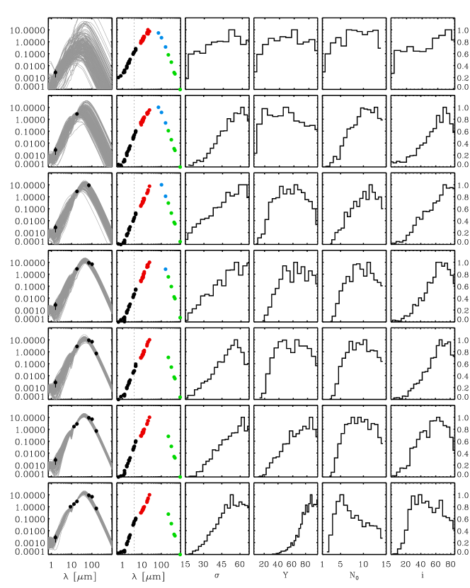
Figure 5: Simulation of a Bayesian adaptive exploration experiment. A new observed point is added in each column from those available for NGC 3081 (Ramos Almeida et al. 2011a). The first column shows the observations with their associated error bars, together with the SEDs obtained from the posterior distribution in each case. The second column shows the expected utility displaying the next best filter. The next four columns represent the marginal posteriors of the CLUMPY parameters $\sigma$, $Y$, $N_{0}$ and $i$, respectively.

At wavelengths $\la$4 $\mu$m we start to see a difference between the expected utilities of Sy1 and Sy2. Optical and NIR observations help constraining the torus parameters for Sy1 (expected utilities between 0.4 and 0.8) more than for Sy2 (expected utilities $\sim$0.2 around 1 $\mu$m). The hot dust emission from the directly illuminated faces of the clumps close to the central engine and the direct AGN emission strongly flatten the Sy1 IR SEDs (see Figure 2). Thus, in the case of Sy1, more observations at short wavelengths are required to constrain the shape of the SED in this region, that in turn constrains parameters such as the inclination angle of the torus ($i$).

As an experiment, we have simulated which is the influence of having a reduced set of observations. To this aim, we have considered the observed points below and above 4 $\mu$m from the complete SEDs. This separation was chosen to roughly separate the NIR and the MIR keeping a similar number of points in both spectral domains. The resulting SEDs are shown in the left and right six panels of Fig. 4 respectively, using the same normalization as in Fig. 2. Again, the grey curves are samples of SEDs using the model parameters from the Bayesian inference. Despite the sparser sampling of the SEDs in the two cases, the results remain essentially similar (see central and right panels of Fig 3), with the expected utility peaking in the 10-200 $\mu$m region. The only difference in the results is a small increase in the expected utitility of the optical and NIR data when only $\lambda>$4 $\mu m$ data is considered in the Sy2 SEDs (bottom right panels in Figure 3).

5 Simulated iterated BAE for NGC 3081

The process we have described until this point is obviously not complete. As already described in Sec. 3, the Bayesian adaptive exploration scheme starts from observations, and then applies Bayesian inference tools to design a new potentially informative observation. Since the typical timescale of this process can be very large given the necessity to apply for observing time in large-aperture telescopes, we have carried out a simulated full process in Fig. 5. We have used the SED of the Sy2 galaxy NGC 3081 presented in Ramos Almeida et al. (2011a). The reason for choosing this galaxy is the availability of Herschel PACS nuclear fluxes. As a first step, we have assumed that we only have the observation in the NICMOS F160W filter and let the Bayesian adaptive exploration scheme select the following filters. BayesClumpy  then uses this point to sample the posterior distribution and obtain marginal posteriors for the clumpy model parameters. The observed point, together with the SEDs sampled from the posterior are shown in the first column of Fig. 5. The second column shows the expected utility, while the remaining panels display the marginal posterior for $\sigma$, $Y$, $N_{0}$ and $i$, respectively.

In order to simulate the next experiment, we have selected the next observation from the set of observed points of the full SED that has the largest expected utility, which turns out to be the T-ReCS Qa data point ($\lambda_{0}=18.3$ $\mu$m). The full process is then repeated until having all the observed points of the SED in the lowest panel. The order in which the remaining filters have been selected is: PACS70, PACS100, PACS160, VISIR NeII_-2 ($\lambda_{0}=13.04$ $\mu$m) and finally, T-ReCS Si2 ($\lambda_{0}=8.72$ $\mu$m). Given that the differences in expected utility are quite small and can change a little because of the inherently random character of the Montecarlo sampling done with BayesClumpy  the specific order might change from run to run. In fact, this means that one could choose a filter giving a large expected utility even though it is not the one giving the largest value if observing with this filter is easier for some specific reason.

It is important to note how the marginal posteriors are constrained when augmenting the number of observed points. Once there are two points in the NIR and MIR, the marginal posterior of $\sigma$ is very similar to what we find when considering the full SED. This is not the case for $Y$ and $N_{0}$, that considerably change after introducing the FIR data and the N-band data points (NeII_-2 and Si2 filters). Finally, the FIR does not seem to make any difference to the inclination angle of the torus, $i$, but the addition of the N-band data points –especially the Si2 filter– result in a different posterior shape, favouring intermediate torus inclinations.

6 Conclusions

The CLUMPY models have recently gained much success on explaining the observed IR SED of the inner parsecs of nearby Seyfert galaxies. Given the observational difficulty (one needs to obtain good signal-to-noise IR photometry of sources at subarcsecond resolution, and ideally, spectroscopy), the sampling of the SEDs is generally quite scarce. Assuming that the CLUMPY models are successful in explaining the observed SED, we have applied a Bayesian adaptive exploration scheme to propose new observations given the presently available information about a source. The results quantitatively indicate that the region between 10 and 200 $\mu$m is crucial, almost independently of the presently available observed points. We also find that optical and NIR data have higher expected utilities in the case of Sy1 than in Sy2. Finally, data from 200 to 500 $\mu$m are found to be useful, even if not as much as data in the 10-200 $\mu$m range, for constraining the torus model parameters. It is important to note that, for simplicity, here we are not considering the angular resolution provided by the different instruments. Thus, aside from the measured expected utility of a given filter, it is important to consider the resolution of the data when deciding the next observation.

We performed a BAE experiment for the galaxy NGC 3081 and found that having two data points only –one in the NIR and another in the MIR– significantly constrains the the torus width ($\sigma$), which does not change when adding further IR data points. The addition of FIR data helps constraining the torus radial extent ($Y$) and the number of clouds (N₀). Finally, the combination of the J, Si2 and Q filters appears to be the most suitable to constrain the inclination angle of the torus ($i$). Note, however, that these are the results found for a particular galaxy, and they may not be applicable to all Seyferts.

Given the large pressure on large-aperture telescopes, our approach –when combined with spatial resolution considerations– is very promising for constraining CLUMPY models, and possibly torus models in general, in sparsely sampled SEDs with the smallest number of observed points. The Bayesian adaptive exploration scheme can be applied to any parametric model (e.g., smooth torus, light curves of classical eclipsing binaries, x-ray binaries) once the tools to carry out a fully Bayesian inference are available. The application to the CLUMPY models is straightforward thanks to the BayesClumpy tool. We note that the computation of the expected utility is already included in the public version of BayesClumpy, which is available for the community.

References

- Alonso-Herrero et al. (2011) Alonso-Herrero A. et al., 2011, ApJ, 736, 82
- Alonso-Herrero et al. (2012a) Alonso-Herrero A., Pereira-Santaella M., Rieke G. H., Rigopoulou D., 2012a, ApJ, 744, 2
- Alonso-Herrero et al. (2012b) Alonso-Herrero A. et al., 2012b, MNRAS, 425, 311
- Antonucci (1993) Antonucci R., 1993, ARA&A, 31, 473
- Asensio Ramos & Ramos Almeida (2009) Asensio Ramos A., Ramos Almeida C., 2009, ApJ, 696, 2075
- Berger (1985) Berger J. O., 1985, Statistical Decision Theory and Bayesian Analysis. Springer-Verlag, New York
- Bishop (2006) Bishop C. M., 2006, Pattern Recognition and Machine Learning. Spinger, New York
- Chiar et al. (2000) Chiar J. E., Tielens A. G. G. M., Whittet D. C. B., Schutte W. A., Boogert A. C. A., Lutz D., van Dishoeck E. F., Bernstein M. P., 2000, ApJ, 537, 749
- Gregory (2005) Gregory P. C., 2005, Bayesian Logical Data Analysis for the Physical Sciences. Cambridge University Press, Cambridge
- Hönig et al. (2006) Hönig S. F., Beckert T., Ohnaka K., Weigelt G., 2006, A&A, 452, 459
- Hönig et al. (2010) Hönig S. F., et al., 2010, A&A, 515, 23
- Hönig et al. (2012) Hönig S. F., Kishimoto M., Antonucci R., Marconi A., Prieto M. A., Tristram K., Weigelt G., 2012, ApJ, 755, 149
- Horst et al. (2009) Horst H., Duschl W. J., Gandhi P., Smette A., 2009, A&A, 495, 137
- Horst et al. (2008) Horst H., Gandhi P., Smette A., Duschl W. J., 2008, A&A, 479, 389
- Jaffe et al. (2004) Jaffe W., et al., 2004, Nature, 429, 47
- Kishimoto et al. (2011) Kishimoto M., Hönig S. F., Antonucci R., Millour F., Tristram, K. R. W., Weigelt, G., 2011, A&A, 536, 78
- Krolik & Begelman (1988) Krolik J. H., Begelman M. C., 1988, ApJ, 329, 702
- Lindley (1956) Lindley D. V., 1956, Ann. Stat., 27, 986
- Loredo (2004) Loredo T. J., 2004, in 23rd International Workshop on Bayesian Inference and Maximum Entropy Methods in Science and Engineering, Vol. 707, Bayesian adaptive exploration, Zhai G. J. E. . Y., ed., AIP, pp. 330–346
- Mason et al. (2006) Mason R. E., Geballe T. R., Packham C., Levenson N. A., Elitzur M., Fisher R. S., Perlman E., 2006, ApJ, 640, 612
- Mason et al. (2009) Mason R. E., Levenson N. A., Shi Y., Packham C., Gorjian V., Cleary K., Rhee J., Werner M., 2009, ApJ, 693, L136
- Mor et al. (2009) Mor R., Netzer H., Elitzur M., 2009, ApJ, 705, 298
- Mor & Netzer (2012) Mor R., Netzer H., 2009, ApJ, 420, 526
- Nenkova et al. (2002) Nenkova M., Ivezić v., Elitzur M., 2002, ApJL, 570, L9
- Nenkova et al. (2008a) Nenkova M., Sirocky M. M., Ivezić v., Elitzur M., 2008a, ApJ, 685, 147
- Nenkova et al. (2008b) Nenkova M., Sirocky M. M., Nikutta R., Ivezić v., Elitzur M., 2008b, ApJ, 685, 160
- Nikutta et al. (2009) Nikutta R., Elitzur M., Lacy M., 2009, ApJ, 707, 1550
- Packham et al. (2005) Packham C., Radomski J. T., Roche P. F., Aitken D. K., Perlman E., Alonso-Herrero A., Colina L., Telesco C. M., 2005, ApJ, 618, L17
- Pier & Krolik (1992) Pier E. A., Krolik J. H., 1992, ApJ, 401, 99
- Pier & Krolik (1993) Pier E. A., Krolik J. H., 1993, ApJ, 418, 673
- Press et al. (1986) Press W. H., Teukolsky S. A., Vetterling W. T., Flannery B. P., 1986, Numerical Recipes. Cambridge University Press, Cambridge
- Radomski et al. (2008) Radomski J. T. et al., 2008, ApJ, 681, 141
- Ramos Almeida et al. (2009) Ramos Almeida C., et al., 2009, ApJ, 702, 1127
- Ramos Almeida et al. (2011a) Ramos Almeida C., et al., 2011a, MNRAS, 417, L46
- Ramos Almeida et al. (2011b) Ramos Almeida C., et al., 2011b, ApJ, 731, 92
- Schartmann et al. (2008) Schartmann M., Meisenheimer K., Camenzind M., Wolf S., Tristram K. R. W., Henning T., 2008, A&A, 482, 67
- Sebastiani & Wynn (2000) Sebastiani P., Wynn H. P., 2000, J. R. Statist. Soc. B, 62, 145
- Tristram et al. (2007) Tristram K. R. W. et al., 2007, A&A, 474, 837
- Urry & Padovani (1995) Urry C. M., Padovani P., 1995, pasp, 107, 803
- Young et al. (2012) Young E. T. et al., 2012, ApJL, 749, L17