Cubic Augmentation of Planar Graphs

Abstract

In this paper we study the problem of augmenting a planar graph such that it becomes 3-regular and remains planar. We show that it is NP-hard to decide whether such an augmentation exists. On the other hand, we give an efficient algorithm for the variant of the problem where the input graph has a fixed planar (topological) embedding that has to be preserved by the augmentation. We further generalize this algorithm to test efficiently whether a 3-regular planar augmentation exists that additionally makes the input graph connected or biconnected. If the input graph should become even triconnected, we show that the existence of a 3-regular planar augmentation is again NP-hard to decide.

1 Introduction

An augmentation of a graph $G=(V,E)$ is a set $W\subseteq E^{c}$ of edges of the complement graph. The augmented graph $G^{\prime}=(V,E\cup W)$ is denoted by $G+W$. We study several problems where the task is to augment a given planar graph to be 3-regular while preserving planarity. The problem of augmenting a graph with the goal that the resulting graph has some additional properties is a well-studied problem and has applications in network planning [et-ap-76]. Often the goal is to increase the connectivity of the graph while adding few edges. Nagamochi and Ibaraki [ni-gcaam-02] study the problem making a graph biconnected by adding few edges. Watanabe and Nakamura [wn-ecap-87] give an $O(c\min\{c,n\}n^{4}(cn+m))$ algorithm for minimizing the number of edges to make a graph $c$-edge-connected. The problem of biconnecting a graph at minimum cost is NP-hard, even if all weights are in $\{1,2\}$ [ni-gcaam-02]. Motivated by graph drawing algorithms that require biconnected input graphs, Kant and Bodlaender [kb-pgap-91] initiated the study of augmenting the connectivity of planar graphs, while preserving planarity. They show that minimizing the number of edges for the biconnected case is NP-hard and give efficient 2-approximation algorithms for both variants. Rutter and Wolff [rw-acpgg-12] give a corresponding NP-hardness result for planar 2-edge connectivity and study the complexity of geometric augmentation problems, where the input graph is a plane geometric graph and additional edges have to be drawn as straight-line segments. Abellanas et al. [aghtu-acgg-08], Tóth [t-capsl-08] and Al-Jubeh et al. [airst-ecap-09] give upper bounds on the number of edges required to make a plane straight-line graph $c$-connected for $c=2,3$. For a survey on plane geometric graph augmentation see [ht-pga-12].

We study the problem of augmenting a graph to be 3-regular while preserving planarity. In doing so, we additionally seek to raise the connectivity as much as possible. Specifically, we study the following problems.

Problem: Planar 3-Regular Augmentation (PRA)
Instance: Planar graph $G=(V,E)$
Task: Find an augmentation $W$ such that $G+W$ is 3-regular and planar.

Problem: Fixed-Embedding Planar 3-Regular Augmentation (FERA)
Instance: Planar graph $G=(V,E)$ with a fixed planar (topological) embedding
Task: Find an augmentation $W$ such that $G+W$ is 3-regular, planar, and $W$ can be added in a planar way to the fixed embedding of $G$.

Moreover, we study $c$-connected FERA, for $c=1,2,3$, where the goal is to find a solution to FERA, such that the resulting graph additionally is $c$-connected.

Contribution and Outline.

Using a modified version of an NP-hardness reduction by Rutter and Wolff [rw-acpgg-12], we show that PRA is NP-hard; the proof is postponed to Section 6.

Theorem 1.

PRA is NP-complete, even if the input graph is biconnected.

Our main result is an efficient algorithm for FERA and $c$-connected FERA for $c=1,2$. We note that Pilz [p-acg-12] has simultaneously and independently studied the planar 3-regular augmentation problem. He showed that it is NP-hard and posed the question on the complexity if the embedding is fixed. Our hardness proof strengthens his result (to biconnected input graphs) and our algorithmic results answer his open question. We further prove that for $c=3$ $c$-connected FERA is again NP-hard.

We introduce basic notions used throughout the paper in Section 2. We present our results on FERA in Section 3. The problem is equivalent to finding a node assignment that assigns the vertices with degree less than 3 to the faces of the graph, such that for each face $f$ an augmentation exists that can be embedded in $f$ in a planar way and raises the degrees of all its assigned vertices to $3$. We completely characterize these assignments and show that their existence can be tested efficiently. We strengthen our characterizations to the case where the graph should become $c$-connected for $c=1,2$ in Section 4 and show that our algorithm can be extended to incorporate these constraints. In Section 5 and Section 6 we provide the hardness proofs for $3$-connected FERA and PRA.

2 Preliminaries

A graph $G=(V,E)$ is 3-regular if all vertices have degree 3. It is a maxdeg-3 graph if all vertices have at most degree 3. For a vertex set $V$, we denote by $V^{\tiny\leavevmode\hbox to5.04pt{\vbox to5.04pt{\text{[drawing]}}}},V^{\tiny\leavevmode\hbox to5.04pt{\vbox to5.04pt{\text{[drawing]}}}}$ and $V^{\tiny\leavevmode\hbox to5.04pt{\vbox to5.04pt{\text{[drawing]}}}}$ the set of vertices with degree 0,1 and 2, respectively. For convenience, we use $V^{\tiny\leavevmode\hbox to4.37pt{\vbox to4.37pt{\text{[drawing]}}}}=V^{\tiny\leavevmode\hbox to5.04pt{\vbox to5.04pt{\text{[drawing]}}}}\cup V^{\tiny\leavevmode\hbox to5.04pt{\vbox to5.04pt{\text{[drawing]}}}}\cup V^{\tiny\leavevmode\hbox to5.04pt{\vbox to5.04pt{\text{[drawing]}}}}$ to denote the set of vertices with degree less than 3. Clearly, an augmentation $W$ such that $G+W$ is 3-regular must contain $3-i$ edges incident to a vertex in $V^{\tiny\leavevmode\hbox to4.54pt{\vbox to4.54pt{\text{[drawing]}}}}$. We say that a vertex $v\in V^{\tiny\leavevmode\hbox to4.54pt{\vbox to4.54pt{\text{[drawing]}}}}$ has $3-i$ (free) valencies and that an edge of an augmentation incident to $v$ satisfies a valency of $v$. Two valencies are adjacent if their vertices are adjacent.

Recall that a graph $G$ is connected if it contains a path between any pair of vertices, and it is $c$-(edge)-connected if it is connected and removing any set of at most $c-1$ vertices (edges) leaves $G$ connected. A 2-connected graph is also called biconnected. We note that the notions of $c$-connectivity and $c$-edge-connectivity coincide on maxdeg-3 graphs. Hence a maxdeg-3 graph is biconnected if and only if it is connected and does not contain a bridge, i.e., an edge whose removal disconnects the graph.

A graph is planar if it admits a planar embedding into the Euclidean plane, where each vertex (edge) is mapped to a distinct point (Jordan curve between its endpoints) such that curves representing distinct edges do not cross. A planar embedding of a graph subdivides the Euclidean plane into faces. When we seek a planar augmentation preserving a fixed embedding, we require that the additional edges can be embedded into these faces in a planar way.

3 Planar 3-Regular Augmentation with Fixed Embedding

In this section we study the problem FERA of deciding for a graph $G=(V,E)$ with fixed planar embedding, whether there exists an augmentation $W$ such that $G+W$ is 3-regular and the edges in $W$ can be embedded into the faces of $G$ in a planar way.

An augmentation $W$ is valid only if the endpoints of each edge in $W$ share a common face in $G$. We assume that a valid augmentation is associated with a (not necessarily planar) embedding of its edges into the faces of $G$ such that each edge is embedded into a face shared by its endpoint. A valid augmentation is planar if the edges can be further embedded in a planar way into the faces of $G$.

Let $F$ denote the set of faces of $G$ and recall that $V^{\tiny\leavevmode\hbox to4.37pt{\vbox to4.37pt{\text{[drawing]}}}}$ is the set of vertices with free valencies. A node assignment is a mapping $A\colon V^{\tiny\leavevmode\hbox to4.37pt{\vbox to4.37pt{\text{[drawing]}}}}\to F$ such that each $v\in V^{\tiny\leavevmode\hbox to4.37pt{\vbox to4.37pt{\text{[drawing]}}}}$ is incident to $A(v)$. Each valid 3-regular augmentation $W$ induces a node assignment by assigning each vertex $v$ to the face where its incident edges in $W$ are embedded: this is well-defined since vertices in $V^{\tiny\leavevmode\hbox to5.04pt{\vbox to5.04pt{\text{[drawing]}}}}\cup V^{\tiny\leavevmode\hbox to5.04pt{\vbox to5.04pt{\text{[drawing]}}}}$ are incident to a single face. A node assignment is realizable if there exists a valid augmentation that induces it. It is realizable in a planar way if it is induced by some planar augmentation. We also call the corresponding augmentation a realization. A realizable node assignment can be found efficiently by computing a matching in the subgraph of $G^{c}$ that contains edges only between vertices that share a common face. The existence of such a matching is a necessary condition for the existence of a planar realization. The main result of this section is that this condition is also sufficient.

Both valid augmentations and node assignments are local by nature, and can be considered independently for distinct faces. Let $A$ be a node assignment and let $f$ be a face. We denote by $V_{f}$ the vertices that are assigned to $f$. We say that $A$ is realizable for $f$ if there exists an augmentation $W_{f}\subseteq\binom{V_{f}}{2}$ such that in $G+W_{f}$ all vertices of $V_{f}$ have degree 3. It is realizable for $f$ in a planar way if additionally $W_{f}$ can be embedded in $f$ without crossings. We call the corresponding augmentations (planar) realizations for $f$. The following lemma is obtained by glueing (planar) realizations for all faces.

Lemma 1.

A node assignment is realizable (in a planar way) for a graph $G$ if and only if it is realizable (in a planar way) for each face $f$ of $G$.

Proof.

Consider a node assignment $A$. If $A$ is realizable (in a planar way), there exists a corresponding valid (planar) augmentation $W$. Then for each face $f$ the set $W_{f}\subseteq W$ of edges embedded in $f$ forms a (planar) realization for $f$. Conversely, assume that $A$ is realizable (in a planar way) for each face $f$. Then for each face $f$ there is a corresponding (planar) realization $W_{f}$ of $A$ for $f$. Hence $W:=\bigcup_{f\in F}W_{f}$ is a valid (planar) augmentation that realizes $A$. ∎

Note that a node assignment induces a unique corresponding assignment of free valencies, and we also refer to the node assignment as assigning free valencies to faces. In the spirit of the notation $G+W$ we use $f+W_{f}$ to denote the graph $G+W_{f}$, where the edges in $W_{f}$ are embedded into the face $f$. If $W_{f}$ consists of a single edge $e$, we write $f+e$. For a fixed node assignment $A$ we sometimes consider an augmentation $W_{f}$ that realizes $A$ for $f$ only in parts by allowing that some vertices assigned to $f$ have still a degree less than 3 in $f+W_{f}$. We then seek an augmentation $W_{f}^{\prime}$ such that $W_{f}\cup W_{f}^{\prime}$ forms a realization of $A$ for $f$. We interpret $A$ as a node assignment for $f+W_{f}$ that assigns to $f$ all vertices that were originally assigned to $f$ by $A$ and do not yet have degree 3 in $f+W_{f}$. Observe that in doing so, we still assign to the faces of $G$ but when considering free valencies and adjacencies, we consider $G+W_{f}$.

3.1 (Planarly) Realizable Assignments for a Face

Throughout this section we consider an embedded graph $G$ together with a fixed node assignment $A$ and a fixed face $f$ of $G$. The goal of this section is to characterize when $A$ is realizable (in a planar way) for $f$. We first collect some necessary conditions for a realizable assignment.

Condition 1 (parity).

The number of free valencies assigned to $f$ is even.

Furthermore, we list certain indicator sets of vertices assigned to $f$ that demand additional valencies outside the set to which they can be matched, as otherwise an augmentation is impossible. Note that these sets may overlap.

1. Joker: A vertex in $V^{\tiny\leavevmode\hbox to5.04pt{\vbox to5.04pt{\text{[drawing]}}}}$ whose neighbors are not assigned to $f$ demands one valency.

2. Pair: Two adjacent vertices in $V^{\tiny\leavevmode\hbox to5.04pt{\vbox to5.04pt{\text{[drawing]}}}}$ demand two valencies.

3. Leaf: A vertex in $V^{\tiny\leavevmode\hbox to5.04pt{\vbox to5.04pt{\text{[drawing]}}}}$ whose neighbor has degree 3 demands two valencies from two distinct vertices.

4. Branch: A vertex in $V^{\tiny\leavevmode\hbox to5.04pt{\vbox to5.04pt{\text{[drawing]}}}}$ and an adjacent vertex in $V^{\tiny\leavevmode\hbox to5.04pt{\vbox to5.04pt{\text{[drawing]}}}}$ demand three valencies from at least two distinct vertices with at most one valency adjacent to the vertex in $V^{\tiny\leavevmode\hbox to5.04pt{\vbox to5.04pt{\text{[drawing]}}}}$.

5. Island: A vertex in $V^{\tiny\leavevmode\hbox to5.04pt{\vbox to5.04pt{\text{[drawing]}}}}$ demands three valencies from distinct vertices.

6. Stick: Two adjacent vertices of degree 1 demand four valencies of which at most two belong to the same vertex.

7. Two vertices in $V^{\tiny\leavevmode\hbox to5.04pt{\vbox to5.04pt{\text{[drawing]}}}}$ demand four valencies; at most two from the same vertex.

8. 3-cycle: A cycle of three vertices in $V^{\tiny\leavevmode\hbox to5.04pt{\vbox to5.04pt{\text{[drawing]}}}}$ demands three valencies.

Condition 2 (matching).

The demands of all indicator sets formed by vertices assigned to $f$ are satisfied.

Each indicator set contains at most three vertices and provides at least the number of valencies it demands; only sets of type (7) provide more. The demand of a joker is implicitly satisfied by the parity condition. We call an indicator set with maximum demand maximum indicator set, and we denote its demand by $k_{\max}$. Note that $k_{\max}\leq 4$. We observe that inserting edges does not increase $k_{\max}$.

Observation 1.

Inserting an edge $uv$ into $f$ does not increase $k_{\max}$.

Proof.

Let $k$ and $k^{\prime}$ denote $k_{\max}$ before and after the insertion of $uv$, respectively. We show $k^{\prime}\leq k$. If $k^{\prime}=4$, then after the insertion there is a stick or an indicator set of type 7. Since a stick can only be obtained from a set of type 7, we have $k=4$. If $k^{\prime}=3$, then after the insertion there is a branch or an island. Since a branch can only be obtained from an island or a stick, we have $k\geq 3$. If $k^{\prime}=2$, then after the insertion there is a pair or a leaf. Since a pair can only be obtained from two leaves, we have $k\geq 2$. ∎

The following lemma reveals the special role of maximum indicator sets.

Lemma 2.

Let $S$ be a maximum indicator set in $f$. Then $A$ satisfies the matching condition for $f$ if and only if the demand of $S$ is satisfied.

Proof.

Clearly, if $A$ satisfies the matching condition than in particular the demand of $S$ is satisfied. Hence, assume that the demand of $S$ is satisfied. We prove that for any indicator set $U$ of vertices assigned to $f$ the demands are satisfied. Observe that the demand of an indicator set that is contained in $S$ is trivially satisfied, we may thus assume that $U$ contains vertices outside of $S$. We distinguish cases based on the demand $k_{\max}$ of $S$.

Case I: $k_{\max}=4$. Then $S$ consists either of a stick or a set of type (7), which is a pair of isolated vertices. Let $U$ be any indicator set distinct from $S$. Assume that $U$ demands four vertices. If $U$ is disjoint from $S$, then $S$ provides the demanded valencies. Otherwise, both $S$ and $U$ consist of a pair of isolated vertices, and they share a common vertex. Since the demand of $S$ is satisfied, there are at least two more assigned valencies provided by vertices outside of $S\cup U$. Together with $S\setminus U$, they provide the demanded valencies for $U$. The same argument applies if $U$ consists of an island, and hence demands three valencies.

If $U$ demands three or fewer valencies and it is not an isolated vertex, then it is either contained in $S$ or disjoint from it. In the former case its demand is satisfied, in the latter case the demand is satisfied by $S$ since an island, which is contained in $S$, is the only indicator set demanding valencies from three different vertices.

Case II: $k_{\max}=3$. Then $S$ consists either of a 3-cycle, an island, or a branch. If $S$ is a 3-cycle, then any other indicator set is either completely contained in $S$ or disjoint from it, and it hence provides the necessary valencies (even for an isolated vertex).

If $S$ consists of an island $s$, observe that $k_{\max}=3$ implies that there is no other island assigned to $f$. The island $s$ provides the necessary valencies for all indicator sets, except for a branch or a leaf. Assume that $U$ is a branch. Since $s$ demands three valencies from distinct vertices, there is a vertex $v\notin U\cup\{s\}$ assigned to $f$. Together $s$ and $v$ provide the valencies for $U$. The case that $U$ is a leaf can be treated analogously.

Finally, consider the case that $S$ consists of a branch. If $U$ consists of an island $u$, then there must be a vertex $v\notin S\cup\{u\}$ providing a valency. Then $S\cup\{v\}$ provide the demanded valencies for $u$. If $U$ is not an island, it demands at most three valencies from at most two different vertices. Hence, if $U$ is disjoint from $S$, $S$ provides the demanded valencies for $U$. It remains to deal with the case that $U$ is a branch sharing its degree-2 vertex with $S$. But then the situation for $U$ and $S$ is completely symmetric, and the demands for $U$ are satisfied.

Case III: $k_{\max}=2$. Since the demands of jokers are always satisfied due to the parity condition, in this case all indicator sets consists either of pairs or of leaves. If $S$ and $U$ are both leaves, their situation is again completely symmetric. If $S$ and $U$ are a leaf and a pair, respectively, they mutually satisfy their demands. It remains to deal with the case that $S$ and $U$ both consist of pairs. If $S$ and $U$ are disjoint, they mutually satisfy their demands. If they share a vertex $S$ and $U$ are again completely symmetric. ∎

The necessity of the parity and the matching condition is obvious; we prove that they are also sufficient for a node assignment to be realizable for $f$.

Theorem 2.

$A$ is realizable for $f$ $\Leftrightarrow$ $A$ satisfies the parity and matching condition for $f$.

The following proof of Theorem 2 postpones the case that $A$ assigns less than seven vertices to $f$ to Lemma 3, which handles this by a case distinction.

Proof.

If $A$ assigns less than seven vertices to $f$, the statement follows from Lemma 3. Moreover, the parity condition and the matching condition are necessary. In the following we assume that $A$ assigns at least seven vertices to $f$ and satisfies the parity condition and the matching condition for $f$. Suppose there exists a partial augmentation $W_{1}$ of $f$ such that $A$ still assigns $k\geq 6$ vertices to $f+W_{1}$ and each assigned vertex has degree 2. We define the graph $H^{c}$ that consists of the vertices assigned to $f+W_{1}$ and contains an edge between two vertices if and only if they are not adjacent in $f+W_{1}$. Since each assigned vertex in $f+W_{1}$ has degree 2, it has at most two adjacencies in $f+W_{1}$ and at least $k-1-2=k-3\geq k/2$ (for $k\geq 6$) adjacencies in $H^{c}$. Thus, by a theorem of Dirac [d-stag-52], a Hamiltonian cycle exists in $H^{c}$, which induces a perfect matching $W_{2}$ of the degree-2 vertices in $f+W_{1}$. Hence $W_{1}\cup W_{2}$ is a 3-regular augmentation for $f$. In the remainder of this proof we show that such a partial augmentation $W_{1}$ always exists.

We begin with the following observation. Let $S$ denote an island or a stick and let $e$ denote an edge between two valencies in $f$. Splitting $e$ and connecting the resulting half-edges to the vertex, respectively the vertices, in $S$ yields an augmentation $\{e_{1},e_{2}\}$ such that the vertices in $S$ have degree 2 in $f+\{e_{1},e_{2}\}$. We refer to this procedure as clipping in $S$.

In the following we construct a partial augmentation $W_{1}$ for all possible assignments for $f$. In order to identify pairs of degree-0 vertices with sticks, in a first step we arbitarily choose pairs of degree-0 vertices and connect them by an edge. Note, that this in particular means that there remains at most one island assigned to $f$. Then we distinguish the possible assignments by the number of degree-1 vertices that are involved in a leaf or a branch. We denote the set of these vertices by $X^{\tiny\leavevmode\hbox to5.04pt{\vbox to5.04pt{\text{[drawing]}}}}$. Since the vertices in $X^{\tiny\leavevmode\hbox to5.04pt{\vbox to5.04pt{\text{[drawing]}}}}$ are mutually non-adjacent, each edge between two of these vertices may occur in $W_{1}$.

For $|X^{\tiny\leavevmode\hbox to5.04pt{\vbox to5.04pt{\text{[drawing]}}}}|>1$ we hence connect the vertices in $X^{\tiny\leavevmode\hbox to5.04pt{\vbox to5.04pt{\text{[drawing]}}}}$ pairwise and clip in possibly existing sticks and islands according to the observation above. If $|X^{\tiny\leavevmode\hbox to5.04pt{\vbox to5.04pt{\text{[drawing]}}}}|$ is odd there remains one vertex $x\in X^{\tiny\leavevmode\hbox to5.04pt{\vbox to5.04pt{\text{[drawing]}}}}$. However, the augmentation constructed so far contains at least one edge, which we split. Then we connect the resulting half-edges to $x$. Thus, $x$ becomes a degree-3 vertex and is no longer assigned. Nevertheless, the condition of six assigned vertices in $f+W_{1}$ is still satisfied since there were at least seven vertices assigned to $f$.

If $|X^{\tiny\leavevmode\hbox to5.04pt{\vbox to5.04pt{\text{[drawing]}}}}|=1$, let $x$ denote the unique vertex in $X^{\tiny\leavevmode\hbox to5.04pt{\vbox to5.04pt{\text{[drawing]}}}}$. As $A$ satisfies the matching condition for $f$, there is at least one vertex $u$ outside the indicator set of $x$ to which we can connect $x$. Thus, $x$ becomes a degree-2 vertex. If $u$ becomes a degree-3 vertex, it is no longer assigned. However, according to the same argument as before, this is no problem. If $u$ was a vertex in a stick or an island, connecting $x$ to $u$ yields a new degree-1 vertex in $X^{\tiny\leavevmode\hbox to5.04pt{\vbox to5.04pt{\text{[drawing]}}}}$ replacing $x$. In this case, we repeat the procedure above until no new degree-1 vertex comes up in $X^{\tiny\leavevmode\hbox to5.04pt{\vbox to5.04pt{\text{[drawing]}}}}$. The resulting matching contains at least one edge and we clip in sticks and islands.

If $|X^{\tiny\leavevmode\hbox to5.04pt{\vbox to5.04pt{\text{[drawing]}}}}|=0$, there exist no leaves and no branches. The only vertices whose degrees need to be increased by $W_{1}$ are those in sticks or islands. All other assigned vertices have degree 2. Let $n^{\prime}$ denote the number of assigned islands and sticks. If $n^{\prime}=1$, there are at least six, respectively seven, further degree-2 vertices assigned since in total A assigns at least seven vertices to $f$ and satisfies the parity condition. In both cases this yields at least eight assigned vertices. We can hence connect the stick or the island with two degree-2 vertices, still having at least six assigned vertices in $f+W_{1}$. If $n^{\prime}\geq 2$ we connect two arbitrary indicator sets, which are either two sticks or a stick and an island, in the obvious way such that each vertex has degree 2 afterwards. All further sticks or islands are then clipped in. Hence in each case we find a corresponding partial augmentation $W_{1}$, which concludes the proof. ∎

Lemma 3.

Let $A$ assign less that seven vertices to $f$. $A$ is realizable for $f$ $\Leftrightarrow$ $A$ satisfies the parity and matching condition for $f$.

Proof.

Let $V_{f}$ denote the vertices assigned to $f$. Recall that $V^{\tiny\leavevmode\hbox to4.54pt{\vbox to4.54pt{\text{[drawing]}}}}_{f}$ then denotes the number of vertices in $V_{f}$ with degree $i$. By assumption, we have $|V^{\tiny\leavevmode\hbox to5.04pt{\vbox to5.04pt{\text{[drawing]}}}}_{f}|+|V^{\tiny\leavevmode\hbox to5.04pt{\vbox to5.04pt{\text{[drawing]}}}}_{f}|+|V^{\tiny\leavevmode\hbox to5.04pt{\vbox to5.04pt{\text{[drawing]}}}}_{f}|\leq 6$. We denote again the maximum number of valencies demanded by any indicator set by $k_{\max}$, and by assumption $A$ satisfies the parity condition and the demands of all indicator sets. At the beginning we show how to solve the following basic situation. Consider a set $N$ of four degree-1 vertices $u_{1},u_{2},u_{3}$ and $u_{4}$, possibly belonging to larger indicator sets, and an even number of at most six free valencies provided by at most two vertices $v_{1}$ and $v_{2}$ not in $N$. Figure 1 shows the only possible occurrences of this situation together with a 3-regular augmentation. We now reduce more complicated situations to these cases.

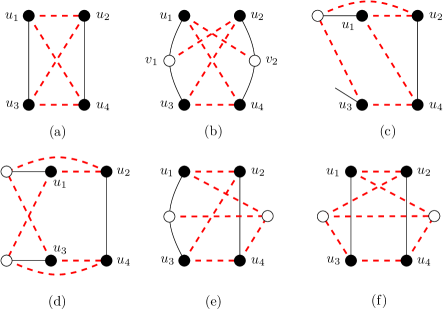
Figure 1: Basic case of Lemma 3. The possible occurrences of four degree-1 vertices in $N$ (black disks) and an even number of up to six free valencies provided by at most two further vertices $v_{1},v_{2}$. For each case a corresponding augmentation (dashed edges) is shown. The black adjacencies are possible but not necessarily present, which only yields simpler situations. (a) no further valencies. (b) two valencies by two further vertices. This augmentation also applies if $v_{1}$ and $v_{2}$ are adjacent. (c) two valencies by one vertex. (d) four valencies by two degree-1 vertices. (e) four valencies by a degree-0 and a degree-2 vertex. Inserting $v_{1}v_{2}$ yields (c). (f) six valencies by two vertices. Inserting $v_{1}v_{2}$ yields (d).

Case 1: $|V^{\tiny\leavevmode\hbox to5.04pt{\vbox to5.04pt{\text{[drawing]}}}}_{f}|\geq 4$. Consider two pairs of degree-0 vertices and connect each pair by an edge. This yields four degree-1 vertices in a set $N$. Outside $N$ there is an even number of at most six free valencies, as two further vertices cannot provide more valencies. Thus, we are done according to the basic case above.

Case 2: $2\leq|V^{\tiny\leavevmode\hbox to5.04pt{\vbox to5.04pt{\text{[drawing]}}}}_{f}|\leq 3$. Consider a fixed set $N$ of two degree-0 vertices and connect them by an edge. Let $k$ be the number of assigned valencies outside of $N$. Observe that outside $N$ there are at most four vertices, among them at most one degree-0 vertex. Hence $k\leq 9$. Conversely, the demand of $N$ is satisfied, and hence $k\geq 4$, moreover, $k$ is even by the parity condition. If $k=4$, then the four remaining valencies in $N$ can be arbitrarily matched to those outside $N$ since the vertices in $N$ form a connected component by themselves.

For the case $k=6$, we now distinguish cases based on $|V^{\tiny\leavevmode\hbox to5.04pt{\vbox to5.04pt{\text{[drawing]}}}}_{f}|$. If $|V^{\tiny\leavevmode\hbox to5.04pt{\vbox to5.04pt{\text{[drawing]}}}}_{f}|=2$ there is no additional degree-0 vertex outside $N$. Then any set of at most four vertices providing six valencies outside $N$ contains at least two degree-1 vertices. We add two such vertices to $N$, reducing the valencies outside $N$ to two, and we are done.

If $|V^{\tiny\leavevmode\hbox to5.04pt{\vbox to5.04pt{\text{[drawing]}}}}_{f}|=3$, the additional degree-0 vertex $v$ outside $N$ already provides three valencies outside. To reach a sum of six, besides $v$, there must be either a degree-2 and a degree-1 vertex or three degree-2 vertices outside $N$. In the former case we connect the degree-0 vertex and the degree-2 vertex by an edge yielding another degree-1 vertex, which we add to $N$ together with the remaining degree-1 vertex. This results in the situation of Figure 1(a). This solution also applies for the second case by identifying two degree-2 vertices with the degree-1 vertex in the first case. This concludes the case $k=6$.

Finally, if $k=8$, there are eight free valencies outside the initial set $N$, and hence any set of at most four vertices providing these valencies contains at least two degree-1 vertices, independent of whether $|V^{\tiny\leavevmode\hbox to5.04pt{\vbox to5.04pt{\text{[drawing]}}}}_{f}|=2$ or $|V^{\tiny\leavevmode\hbox to5.04pt{\vbox to5.04pt{\text{[drawing]}}}}_{f}|=3$. Adding two such degree-1 vertices to $N$ reduces the number of valencies outside $N$ to four, and we are done.

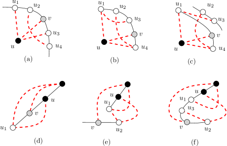
Figure 2: Illustration of the proof of Lemma 3; augmentation edges are dashed. The black vertices form a maximum indicator set $S$ with demand $k_{\max}$, the grey vertex $v$ has degree 2 and exists due to the demand of $S$. All augmentations also apply if the solid adjacencies are (partly) dropped. In (a)-(c) $k_{\max}=3$, and there is a single vertex $u$ of degree-0. (a) $|V^{\tiny\leavevmode\hbox to5.04pt{\vbox to5.04pt{\text{[drawing]}}}}_{f}|=0$, also applies if $u_{1}$ and $u_{4}$ are adjacent or ignored. Moreover $\{u_{1},u_{2}\}$ or $\{u3,u_{4}\}$ may be considered as a single degree-1 vertex. (b) + (c) $|V^{\tiny\leavevmode\hbox to5.04pt{\vbox to5.04pt{\text{[drawing]}}}}_{f}|=2$ and $|V^{\tiny\leavevmode\hbox to5.04pt{\vbox to5.04pt{\text{[drawing]}}}}_{f}|>0$; the augmentation also applies if $\{u_{2},u_{3}\}$ is considered as a single degree-1 vertex. (d)-(f) $k_{\max}=3$ and a branch $S$ with degree-2 vertex $u\in S$. (d) One degree-1 vertex besides $S$ not adjacent to $u$; also applies if $u_{1}$ is considered as two degree-2 vertices. (e) Two degree-1 vertices besides $S$, one adjacent to $u$; also applies if $u_{2}$ is considered as two degree-2 vertices. (f) One degree-1 vertex and further degree-2 vertices besides $S$, adjacent to $u$.

Case 3: $|V^{\tiny\leavevmode\hbox to5.04pt{\vbox to5.04pt{\text{[drawing]}}}}_{f}|=1$. Let $u$ denote the only degree-0 vertex, which demands three further valencies from distinct vertices, that is, $k_{\max}\in\{3,4\}$, and there are at least three vertices assigned besides $u$ of which at least one vertex $v$ is of degree 2 in order to satisfy the parity condition. More precisely, there is an even positive number of valencies provided by two, three or four vertices besides $u$ and $v$, as the total number of vertices assigned to $f$ is at most six. We distinguish cases based on the demand $k_{\max}$.

If $k_{\max}=3$, consider the number of assigned degree-1 vertices. Recall that the degree-1 vertices are pairwise non-adjacent, $k_{\max}$ would be 4, otherwise. If $|V^{\tiny\leavevmode\hbox to5.04pt{\vbox to5.04pt{\text{[drawing]}}}}_{f}|=0$, the demand of $u$ implies that $V\setminus\{u,v\}$ consists of at least two degree-2 vertices. It follows from the parity condition that the number of these degree-2 vertices is either two or four. Figure 2(a) shows a solution for four further degree-2 vertices. The case of only two further degree-2 vertices can be deduces from Figure 2(a) by ignoring $u_{2}$ and $u_{4}$. If $|V^{\tiny\leavevmode\hbox to5.04pt{\vbox to5.04pt{\text{[drawing]}}}}_{f}|=1$, the demand of $u$ and the parity condition imply that there are exactly two degree-2 vertices in $V_{f}\setminus\{u,v\}$. An augmentation is given by Figure 2(a) identifying $u_{1}$ and $u_{2}$ with the degree-1 vertex. If $|V^{\tiny\leavevmode\hbox to5.04pt{\vbox to5.04pt{\text{[drawing]}}}}_{f}|=2$, we have $|V^{\tiny\leavevmode\hbox to5.04pt{\vbox to5.04pt{\text{[drawing]}}}}_{f}\setminus\{v\}|\leq 2$ and even. This situation is solved by Figure 2(b) and (c). If there are no additional degree-2 vertices an augmentation results from Figure 2(a) by identifying $u_{1}$ and $u_{2}$ as well as $u_{3}$ and $u_{4}$ with the two degree-1 vertices (which are non-adjacent). If $|V^{\tiny\leavevmode\hbox to5.04pt{\vbox to5.04pt{\text{[drawing]}}}}_{f}|=3$, the parity condition prohibits a further degree-2 vertex. Thus, Figure 2(c) provides an augmentation by identifying $u_{2}$ and $u_{3}$ with a degree-1 vertex not adjacent to $u_{1}$ and $u_{4}$. The case $|V^{\tiny\leavevmode\hbox to5.04pt{\vbox to5.04pt{\text{[drawing]}}}}_{f}|=4$ is shown by Figure 1(e), ignoring the adjacency of $u_{2}$ and $u_{4}$.

If $k_{\max}=4$, there must exist at least one stick $S$ that demands four additional valencies, of which at most two belong to the same vertex. This is, besides $S$, $u$ and $v$, there is an even positive number of valencies provided by at most two further vertices. If $|V^{\tiny\leavevmode\hbox to5.04pt{\vbox to5.04pt{\text{[drawing]}}}}_{f}|\geq 4$, we are in the situation of Figure 1(e). If $|V^{\tiny\leavevmode\hbox to5.04pt{\vbox to5.04pt{\text{[drawing]}}}}_{f}|=3$, the parity condition prohibits a further degree-2 vertex. This situation can be deduced from of Figure 2(c) assuming $u_{1}$ and $u_{4}$ are adjacent, forming $S$, and identifying $u_{2}$ and $u_{3}$ with the degree-1 vertex; the vertex $v$ may be located arbitrarily. If $|V^{\tiny\leavevmode\hbox to5.04pt{\vbox to5.04pt{\text{[drawing]}}}}_{f}|=2$, $S$ contains the only degree-1 vertices, and there must be two further degree-2 vertices besides $S$, $u$ and $v$. Thus, Figure 2(c) provides a solution assuming $u_{1}$ and $u_{4}$ form $S$ and the remaining degree-2 vertices are located arbitrarily.

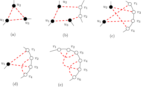
Figure 3: Augmentation (dashed edges) of assignments with $k_{\max}=2$. The black vertices have degree 1. All augmentations also apply if the solid adjacencies are (partly) dropped. (a) $|V^{\tiny\leavevmode\hbox to5.04pt{\vbox to5.04pt{\text{[drawing]}}}}_{f}|=1$; augmentation also applies if $u_{3}$ is considered as two degree-2 vertices. (b) $|V^{\tiny\leavevmode\hbox to5.04pt{\vbox to5.04pt{\text{[drawing]}}}}_{f}|=3$ and $|V^{\tiny\leavevmode\hbox to5.04pt{\vbox to5.04pt{\text{[drawing]}}}}_{f}|=2$. (c) $|V^{\tiny\leavevmode\hbox to5.04pt{\vbox to5.04pt{\text{[drawing]}}}}_{f}|=2$ and $|V^{\tiny\leavevmode\hbox to5.04pt{\vbox to5.04pt{\text{[drawing]}}}}_{f}|=4$; also applies if $v_{1}$ and $v_{4}$ are adjacent or $u_{2}$, $v_{2}$ and $v_{4}$ are ignored. (d) $|V^{\tiny\leavevmode\hbox to5.04pt{\vbox to5.04pt{\text{[drawing]}}}}_{f}|=1$ and $|V^{\tiny\leavevmode\hbox to5.04pt{\vbox to5.04pt{\text{[drawing]}}}}_{f}|=4$; also applies if $v_{1}$ and $v_{4}$ are adjacent. (e) $|V^{\tiny\leavevmode\hbox to5.04pt{\vbox to5.04pt{\text{[drawing]}}}}_{f}|=6$; also applies if $v_{1}$ and $v_{6}$ are adjacent or $v_{4}$ and $v_{6}$ are ignored.

Case 4: $|V^{\tiny\leavevmode\hbox to5.04pt{\vbox to5.04pt{\text{[drawing]}}}}_{f}|=0$. If $k_{\max}=1$, there is an even number of jokers assigned to $f$. We connect pairs arbitrarily.

If $k_{\max}=2$ and $|V^{\tiny\leavevmode\hbox to5.04pt{\vbox to5.04pt{\text{[drawing]}}}}_{f}|\geq 4$, we are done according to Figure 1(a)-(d). Note that due to $k_{\max}=2$ each degree-1 vertex is neither part of a stick, nor of a branch, and hence is not adjacent to other assigned vertices. For $|V^{\tiny\leavevmode\hbox to5.04pt{\vbox to5.04pt{\text{[drawing]}}}}_{f}|=3$, Fig. 3(a) and (b) show an augmentation, depending on whether the degree-1 vertices are accompanied by two degree-2 vertices or not. Note that the total limit of six vertices and the parity condition does not allow for a different number of degree-2 vertices. If $|^{\tiny\leavevmode\hbox to5.04pt{\vbox to5.04pt{\text{[drawing]}}}}V_{f}|=2$, there are either two or four degree-2 vertices, as otherwise the demands or the parity condition would be violated. Corresponding solutions are given by Figure 3(a) (by identifying $u_{3}$ with two arbitrarily located degree-2 vertices) and Figure 3(c), respectively. If $|V^{\tiny\leavevmode\hbox to5.04pt{\vbox to5.04pt{\text{[drawing]}}}}_{f}|=1$, there are two or four degree-2 vertices. Corresponding augmentations are shown in Figure 3(c) (ignoring $u_{2}$, $v_{2}$ and $v_{4}$) and Figure 3(d), respectively. Finally, if $|V^{\tiny\leavevmode\hbox to5.04pt{\vbox to5.04pt{\text{[drawing]}}}}_{f}|=0$, all valencies assigned to $f$ are provided by degree-2 vertices. Figure 3(e) shows an augmentation for six valencies. Ignoring $v_{4}$ and $v_{6}$ in Figure 3(e) yields an augmentation of four valencies. Augmenting two non-adjacent degree-2 vertices is trivial.

If $k_{\max}=3$, we distinguish cases based on whether there is a 3-cycle assigned to $f$. If this is the case, let $C$ the vertex set of such a cycle. Due to the parity condition there must be a further vertex $v$ of degree 2 assigned to $f$. More precisely, by the demand of $C$ and the parity condition, there is an even positive number of valencies provided by one or two further vertices outside $C\cup\{v\}$. If there are two valencies provided outside $C\cup\{v\}$, we pair the valencies of $C$ arbitrarily with the remaining three valencies. If there are four valencies assigned, then they are provided by two non-adjacent degree-1 vertices. Connecting them by an edge reduces to the previous case. Now assume that there is no 3-cycle, and hence there is a branch $S$ demanding three valencies. Due to the parity condition there is a further degree-2 vertex $v$ assigned to $f$. By the parity condition there is an even positive number of valencies outside $S\cup\{v\}$, which is provided by one, two or three further vertices. We distinguish cases based on the number $k$ of these valencies. Note that $k\leq 6$.

If $k=2$, the valencies are provided by one or two vertices. We note that if it is a degree-1 vertex, then it is not adjacent to $S$, as this would contradict the demand of $S$, and Figure 2(d) shows a solution for this case. The same augmentation works if the valencies are provided by two degree-2 vertices by considering two degree-2 vertices that are not adjacent to $S$ as the single degree-1 vertex $u_{1}$ in the figure. If $k=4$, consider the case that the four valencies outside $S\cup\{v\}$ are provided by two degree-1 vertices. Figure 2(e) shows a solution, and this also holds if $u_{2}$ is replaced by two degree-2 vertices that are located arbitrarily. It remains to deal with the case where four valencies are provided by a degree-1 vertex and two degree-2 vertices, but the degree-1 vertex is adjacent to $S$. Figure 2(e) shows a solution for this case. If $k=6$, all further vertices have degree 1, resulting in $|V^{\tiny\leavevmode\hbox to5.04pt{\vbox to5.04pt{\text{[drawing]}}}}_{f}|=4$, which can be handled by the basic case. This concludes the case $k_{\max}=3$.

If $k_{\max}=4$, let $S\subseteq V^{\tiny\leavevmode\hbox to5.04pt{\vbox to5.04pt{\text{[drawing]}}}}_{f}$ denote a stick. If $|V^{\tiny\leavevmode\hbox to5.04pt{\vbox to5.04pt{\text{[drawing]}}}}_{f}|=4$, we are done according to Figure 1(a)-(d). If $|V^{\tiny\leavevmode\hbox to5.04pt{\vbox to5.04pt{\text{[drawing]}}}}_{f}|=3$, then we have $|V^{\tiny\leavevmode\hbox to5.04pt{\vbox to5.04pt{\text{[drawing]}}}}_{f}|=2$ by the demand of $S$ and the total limit of six vertices. In this case outside $S$ there are exactly the four valencies demanded by $S$, and we may connect them arbitrarily since $S$ forms a connected component. Finally, if $|V^{\tiny\leavevmode\hbox to5.04pt{\vbox to5.04pt{\text{[drawing]}}}}_{f}|=2$, the demand of $S$ must be satisfied by four degree-2 vertices, and we connect $S$ to these vertices arbitrarily. ∎

Given a node assignment $A$ that satisfies the parity and the matching condition for a face $f$, the following rule picks an edge that can be inserted into $f$. Lemma 4 states that afterwards the remaining assignment still satisfies the parity and the matching condition. Iteratively applying Rule 1 hence yields a (not necessarily planar) realization.

Rule 1.

1. If $k_{\max}\geq 3$ let $S$ denote a maximum indicator set. Choose a vertex $u$ of lowest degree in $S$ and connect this to an arbitrary assigned vertex $v\notin S$.

2. If $k_{\max}=2$ and $u$ is a leaf, choose $S=\{u\}$, and connect $u$ to an assigned vertex $v$.

3. If $k_{\max}=2$ and there is no leaf, let $S$ denote a path $xuy$ of assigned vertices in $V^{\tiny\leavevmode\hbox to5.04pt{\vbox to5.04pt{\text{[drawing]}}}}$. Connect $u$ to an arbitrary assigned vertex $v\notin S$.

4. If $k_{\max}=2$ and there is neither a leaf nor a path of three assigned vertices in $V^{\tiny\leavevmode\hbox to5.04pt{\vbox to5.04pt{\text{[drawing]}}}}$, let $S$ denote a pair $uw$. Connect $u$ to an arbitrary assigned vertex $v\notin S$.

5. If $k_{\max}=1$, choose $S=\{u\}$, where $u$ is a joker, and connect $u$ to another joker $v$.

Lemma 4.

Assume $A$ satisfies the parity and matching condition for $f$ and let $e$ denote an edge chosen according to Rule 1. Then $A$ satisfies the same conditions for $f+e$.

Proof.

It follows from Theorem 2 that $A$ is realizable for $f$. Thus, let $W_{f}$ denote a 3-regular augmentation for $f$. If $e=uv\in W_{f}$, we are done since $W_{f}\setminus\{e\}$ is a 3-regular augmentation for $f+e$.

Hence, assume $uv\notin W_{f}$. We consider the set $W^{\footnotesize\leavevmode\hbox to5.32pt{\vbox to5.32pt{\text{[drawing]}}}}\subseteq W_{f}$ of edges that are incident to vertices in $S$, where $S$ is the set determined by the rule. It is $u\in S$ and $v\notin S$ for all rules. The deletion of $W^{\footnotesize\leavevmode\hbox to5.32pt{\vbox to5.32pt{\text{[drawing]}}}}$ in $f+W_{f}$ yields a set $X^{\tiny\leavevmode\hbox to4.37pt{\vbox to4.37pt{\text{[drawing]}}}}\cup S$ of vertices which have again free valencies in $f+(W_{f}-W^{\footnotesize\leavevmode\hbox to5.32pt{\vbox to5.32pt{\text{[drawing]}}}})$. If $v$ is connected to a vertex of $S$ in $W_{f}$, then we already have $v\in X^{\tiny\leavevmode\hbox to4.37pt{\vbox to4.37pt{\text{[drawing]}}}}$. Otherwise, we add an arbitrary edge $vx\in W_{f}$ to $W^{\footnotesize\leavevmode\hbox to5.32pt{\vbox to5.32pt{\text{[drawing]}}}}$, which yields $v,x\in X^{\tiny\leavevmode\hbox to4.37pt{\vbox to4.37pt{\text{[drawing]}}}}$. Clearly, $A$ satisfies the parity condition and the matching condition for $f+(W_{f}-W^{\footnotesize\leavevmode\hbox to5.32pt{\vbox to5.32pt{\text{[drawing]}}}})$, and, after insertion of $e=uv$, at least the parity condition for $f+(W_{f}-W^{\footnotesize\leavevmode\hbox to5.32pt{\vbox to5.32pt{\text{[drawing]}}}})+uv$. In the following we show that $A$ also satisfies the demand of a maximum indicator set $S^{\prime}$ in $f+(W_{f}-W^{\footnotesize\leavevmode\hbox to5.32pt{\vbox to5.32pt{\text{[drawing]}}}})+uv$. Then $A$ satisfies the matching condition for $f+(W_{f}-W^{\footnotesize\leavevmode\hbox to5.32pt{\vbox to5.32pt{\text{[drawing]}}}})+uv$ by Lemma 2, and there exists an augmentation $W^{\oplus}$ for $f+(W_{f}-W^{\footnotesize\leavevmode\hbox to5.32pt{\vbox to5.32pt{\text{[drawing]}}}})+uv$ such that $(W_{f}-W^{\footnotesize\leavevmode\hbox to5.32pt{\vbox to5.32pt{\text{[drawing]}}}})+W^{\oplus}$ is an augmentation for $f+e$. Hence, $A$ satisfies the parity condition and the matching condition for $f+e$ as claimed by the lemma.

For each subrule we distinguish cases based on the type of $S$. Recall that the insertion of edges never increases $k_{\max}$. Thus, any maximum indicator set in $f+(W_{f}-W^{\footnotesize\leavevmode\hbox to5.32pt{\vbox to5.32pt{\text{[drawing]}}}})+uv$ demands at most as many valencies as a maximum indicator set in $f$. Note further, that $v$ has degree 3 in $f+(W_{f}-W^{\footnotesize\leavevmode\hbox to5.32pt{\vbox to5.32pt{\text{[drawing]}}}})+uv$ if $v$ is not matched to $S$ in $W_{f}$.

Subrule 1: In this case, $S$ is a maximum indicator set, and we distinguish further cases based on the exact type of $S$.

Case I: Assume $S$ is a stick or an indicator set of type (7). If $v$ was connected to $s\in S$ in $W_{f}$, then, except for the valency at $s$, which was connected to $u$, the valencies in $X^{\tiny\leavevmode\hbox to4.37pt{\vbox to4.37pt{\text{[drawing]}}}}\setminus(S\cup\{v\})$ were matched to $S$. Due to the symmetry of $S$, these valencies can be also matched to $S$ preserving the necessary valency for $v$ at $u$. Thus, $A$ satisfies the parity condition and the matching condition for $f+e$, according to Theorem 2.

If $v$ was not connected to $S$ in $W_{f}$ and $S$ is a set of type (7), we connect the isolated degree-0 vertices in $S$ by an edge, such that $S$ becomes a stick. Since this does not change the demand of $S$, which remains a maximum indicator set, Lemma 2 and Theorem 2 imply that $A$ is still realizable for $f+(W_{f}-W^{\footnotesize\leavevmode\hbox to5.32pt{\vbox to5.32pt{\text{[drawing]}}}})$ after this insertion. Thus, we identify this case with the next case, where $S$ is a stick.

Assume that $S$ is a stick and $v$ was not connected to $S$ in $W_{f}$. Then $S$ provides three valencies at two distinct vertices in $f+(W_{f}-W^{\footnotesize\leavevmode\hbox to5.32pt{\vbox to5.32pt{\text{[drawing]}}}})+uv$. The vertices with free valencies in $f+(W_{f}-W^{\footnotesize\leavevmode\hbox to5.32pt{\vbox to5.32pt{\text{[drawing]}}}})+uv$ are partitioned into two disjoint, non-adjacent groups, namely $S$ and $X^{\tiny\leavevmode\hbox to4.37pt{\vbox to4.37pt{\text{[drawing]}}}}\setminus(S\cup\{v\})$. We show that no maximum indicator set $S^{\prime}$ contains vertices of both sets, and then argue that the group that has empty intersection with a maximum indicator set $S^{\prime}$ provides enough valencies to satisfy the demand of $S^{\prime}$.

First observe that $S$ and $X^{\tiny\leavevmode\hbox to4.37pt{\vbox to4.37pt{\text{[drawing]}}}}\setminus(S\cup\{v\})$ are disjoint by definition and non-adjacent since $S$ was a stick (before connecting it to $v$). Let $S^{\prime}$ be any maximum indicator set $f+(W_{f}-W^{\footnotesize\leavevmode\hbox to5.32pt{\vbox to5.32pt{\text{[drawing]}}}})+uv$. By definition $S$ does not contain a degree-0 vertex, which could belong to an indicator set of type (7). Since all other indicator sets are connected it follows that either $S^{\prime}\subseteq S$ or $S^{\prime}\cap S=\emptyset$. The set $X^{\tiny\leavevmode\hbox to4.37pt{\vbox to4.37pt{\text{[drawing]}}}}\setminus(S\cup\{v\})$ provides (at least) $4+1=5$ valencies on at least three distinct vertices in $f+(W_{f}-W^{\footnotesize\leavevmode\hbox to5.32pt{\vbox to5.32pt{\text{[drawing]}}}})+uv$. Recall that if $S$ has originally been a set of type (7), it may have induced six valencies provided by $X^{\tiny\leavevmode\hbox to4.37pt{\vbox to4.37pt{\text{[drawing]}}}}\setminus(S\cup\{v\})$ in $f+(W_{f}-W^{\footnotesize\leavevmode\hbox to5.32pt{\vbox to5.32pt{\text{[drawing]}}}})+uv$. The valencies in $X^{\tiny\leavevmode\hbox to4.37pt{\vbox to4.37pt{\text{[drawing]}}}}\setminus(S\cup\{v\})$ clearly satisfy the demand of any maximum indicator set $S^{\prime}\subseteq S$. If $S^{\prime}\subseteq X^{\tiny\leavevmode\hbox to4.37pt{\vbox to4.37pt{\text{[drawing]}}}}\setminus(S\cup\{v\})$, then $S^{\prime}$ either consists of at most two vertices or it is a 3-cycle. In both cases there exists at least one valency in $X^{\tiny\leavevmode\hbox to4.37pt{\vbox to4.37pt{\text{[drawing]}}}}\setminus(S\cup\{v\})$ outside $S^{\prime}$ since $S^{\prime}$ provides at most three valencies. Thus, $S$ together with this valency provides four valencies on at least three distinct vertices, which satisfies the demand of any indicator set $S^{\prime}\subseteq X^{\tiny\leavevmode\hbox to4.37pt{\vbox to4.37pt{\text{[drawing]}}}}\setminus(S\cup\{v\})$.

Case II: Assume $S$ is a 3-cycle or an island. If $v$ was connected to $s\in S$ in $W_{f}$, we are done by the same symmetry argument as in the beginning of Case I.

If $v$ was not connected to $S$ in $W_{f}$, $S$ provides two valencies at at most two distinct vertices in $f+(W_{f}-W^{\footnotesize\leavevmode\hbox to5.32pt{\vbox to5.32pt{\text{[drawing]}}}})+uv$, and again each maximum indicator set $S^{\prime}$ is completely contained either in $S$ or in $X^{\tiny\leavevmode\hbox to4.37pt{\vbox to4.37pt{\text{[drawing]}}}}\setminus(S\cup\{v\})$.

The latter provides $3+1=4$ valencies on at least two distinct vertices in $f+(W_{f}-W^{\footnotesize\leavevmode\hbox to5.32pt{\vbox to5.32pt{\text{[drawing]}}}})+uv$. This clearly satisfies the demand of any maximum indicator set $S^{\prime}\subseteq S$, since $S^{\prime}$ demands at most two valencies in $f+(W_{f}-W^{\footnotesize\leavevmode\hbox to5.32pt{\vbox to5.32pt{\text{[drawing]}}}})+uv$. If $S^{\prime}\subseteq X^{\tiny\leavevmode\hbox to4.37pt{\vbox to4.37pt{\text{[drawing]}}}}\setminus(S\cup\{v\})$, there exists at least one valency in $X^{\tiny\leavevmode\hbox to4.37pt{\vbox to4.37pt{\text{[drawing]}}}}\setminus(S\cup\{v\})$ outside $S^{\prime}$ since each maximum indicator set (for $k_{\max}=3$) provides only three valencies. Thus, $S$ together with this valency provides three valencies at three distinct vertices if $S$ was a 3-cycle (before connecting $u$ and $v$), and at two distinct vertices if $S$ was an island. In both cases this satisfies the demand of any maximum indicator set $S^{\prime}\subseteq X^{\tiny\leavevmode\hbox to4.37pt{\vbox to4.37pt{\text{[drawing]}}}}\setminus(S\cup\{v\})$ with $k_{\max}=3$. Note that in the latter case $S^{\prime}\subseteq X^{\tiny\leavevmode\hbox to4.37pt{\vbox to4.37pt{\text{[drawing]}}}}\setminus(S\cup\{v\})$ is no island since together with $u$ this would have induced a set of type (7) in $f$, contradicting $k_{\max}=3$.

Case III: Assume $S$ is a branch. Recall that $u$ is the degree-1 vertex in $S$. Denote the degree-2 vertex in $S$ by $r$. The second vertex $x$ besides $u$ that is adjacent to $r$ in $f+(W_{f}-W^{\footnotesize\leavevmode\hbox to5.32pt{\vbox to5.32pt{\text{[drawing]}}}})+uv$ has at least degree 2 since $S$ can be connected to this vertex by at most one edge in $W_{f}$. However, unlike the previous cases, it is now possible that a maximum indicator set $S^{\prime}$ has nonempty intersection with both $S$ and $X^{\tiny\leavevmode\hbox to4.37pt{\vbox to4.37pt{\text{[drawing]}}}}\setminus(S\cup\{v\})$. This is the case where $S^{\prime}=\{r,x\}$ and $x$ has degree 2, and we have to consider this case in addition to the usual ones. Observe that $S$ provides two valencies at $u$ and $r$ in $f+(W_{f}-W^{\footnotesize\leavevmode\hbox to5.32pt{\vbox to5.32pt{\text{[drawing]}}}})+uv$.

If $v$ was connected to $r\in S$ in $W_{f}$, $v$ has degree 3 in $f+(W_{f}-W^{\footnotesize\leavevmode\hbox to5.32pt{\vbox to5.32pt{\text{[drawing]}}}})+uv$, as $uv\notin W_{f}$, and $X^{\tiny\leavevmode\hbox to4.37pt{\vbox to4.37pt{\text{[drawing]}}}}\setminus(S\cup\{v\})$ provides exactly two valencies at two degree-2 vertices (the ones that were adjacent to $u$ in $W_{f}$. This clearly satisfies the demand of each maximum indicator set $S^{\prime}\subseteq S$ since in this case $S^{\prime}$ demands at most two vertices. If $S^{\prime}\subseteq X^{\tiny\leavevmode\hbox to4.37pt{\vbox to4.37pt{\text{[drawing]}}}}\setminus(S\cup\{v\})$, then since $S^{\prime}\subseteq X^{\tiny\leavevmode\hbox to4.37pt{\vbox to4.37pt{\text{[drawing]}}}}\setminus(S\cup\{v\})$ consists of two degree-2 vertices, $S^{\prime}$ demands two valencies, which are satisfied by $S$. If $S^{\prime}=\{x,r\}$ is the pair containing vertices of both groups, its demand is satisfied by $u$ and the degree-2 vertex in $X^{\tiny\leavevmode\hbox to4.37pt{\vbox to4.37pt{\text{[drawing]}}}}\setminus(S\cup\{v\})$ different from $x$.

If $v$ was not connected to $r\in S$ in $W_{f}$, $X^{\tiny\leavevmode\hbox to4.37pt{\vbox to4.37pt{\text{[drawing]}}}}\setminus(S\cup\{v\})$ provides $3+1=4$ valencies on at least three vertices, due to $k_{\max}=3$. This clearly satisfies the demand of each maximum indicator set $S^{\prime}\subseteq S$. If $S^{\prime}\subseteq X^{\tiny\leavevmode\hbox to4.37pt{\vbox to4.37pt{\text{[drawing]}}}}\setminus(S\cup\{v\})$, there exists at least one valency in $X^{\tiny\leavevmode\hbox to4.37pt{\vbox to4.37pt{\text{[drawing]}}}}\setminus(S\cup\{v\})$ outside $S^{\prime}$ since each maximum indicator set provides only three valencies. Thus, $S$ together with this valency provides three valencies at three distinct vertices, which satisfies the demand of each maximum set $S^{\prime}\subseteq X^{\tiny\leavevmode\hbox to4.37pt{\vbox to4.37pt{\text{[drawing]}}}}\setminus(S\cup\{v\})$ with $k_{\max}=3$. Finally, if $S^{\prime}=\{r,x\}$ is the pair containing vertices of both groups, the demand of $S^{\prime}$, which is 2, is easily satisfied by the remaining three valencies in $X^{\tiny\leavevmode\hbox to4.37pt{\vbox to4.37pt{\text{[drawing]}}}}\setminus(S\cup\{v\})$. This concludes the treatment of subrule 1.

Subrules 2 and 4: In this case the set $S$ is a leaf or a pair (of adjacent degree-2 vertices), and we have $k_{\max}=2$. If $v$ was matched to $s\in S$ in $W_{f}$, we are done by the same symmetry argument as before.

If $v$ was not matched to $S$ in $W_{f}$, then $S$ provides one valency at one vertex in $f+(W_{f}-W^{\footnotesize\leavevmode\hbox to5.32pt{\vbox to5.32pt{\text{[drawing]}}}})+uv$. Again we argue that each maximum indicator set $S^{\prime}$ is either in $S$ or in $X^{\tiny\leavevmode\hbox to4.37pt{\vbox to4.37pt{\text{[drawing]}}}}\setminus(S\cup\{v\})$. If $S^{\prime}$ is a leaf, this is clear and if it is a pair $\{u,w\}$, that is if subrule 4 is applied, the neighbors of $u$ and $w$ have degree $3$ as subrule 3 would have been applied otherwise. Hence $S$ and $\{u,w\}$ are either equal or disjoint.

The set $X^{\tiny\leavevmode\hbox to4.37pt{\vbox to4.37pt{\text{[drawing]}}}}\setminus(S\cup\{v\})$ provides $2+1=3$ valencies on at least two distinct vertices. This clearly satisfies the demand of each maximum indicator set $S^{\prime}\subseteq S$ since in this case $S^{\prime}$ demands only one valency. If $S^{\prime}\subseteq X^{\tiny\leavevmode\hbox to4.37pt{\vbox to4.37pt{\text{[drawing]}}}}\setminus(S\cup\{v\})$, there exists at least one valency in $X^{\tiny\leavevmode\hbox to4.37pt{\vbox to4.37pt{\text{[drawing]}}}}\setminus(S\cup\{v\})$ outside $S^{\prime}$ since each maximum indicator set (for $k_{\max}=2$) provides only two valencies. Thus, $S$ together with this valency provides two valencies on at least two distinct vertices, which satisfies the demand of each maximum set $S^{\prime}\subseteq X^{\tiny\leavevmode\hbox to4.37pt{\vbox to4.37pt{\text{[drawing]}}}}\setminus(S\cup\{v\})$ with $k_{\max}=2$.

Subrule 5: Since $S$ is a joker, that is $k_{\max}=1$, all vertices in $X^{\tiny\leavevmode\hbox to4.37pt{\vbox to4.37pt{\text{[drawing]}}}}$ are jokers in $f+(W_{f}-W^{\footnotesize\leavevmode\hbox to5.32pt{\vbox to5.32pt{\text{[drawing]}}}})$. Jokers can be matched arbitrarily, and thus, there exists an augmentation that contains $e=uv$. By Theorem 2, $A$ then satisfies the parity condition and the matching condition for $f+e$.

Subrule 3: Subrule 3 differs from the remaining rules since $S$ is no indicator set. Consequently, $W_{f}$ may contain the edge $xy$ between the endpoints of the path forming $S$. If $W_{f}$ does not contain $xy$, then $X^{\tiny\leavevmode\hbox to4.37pt{\vbox to4.37pt{\text{[drawing]}}}}\setminus(S\cup\{v\})$ provides four valencies in $f+(W_{f}-W^{\footnotesize\leavevmode\hbox to5.32pt{\vbox to5.32pt{\text{[drawing]}}}})+uv$ (three for $S$ and one for $v$). If $xy\in W_{f}$, then $S\cup\{v\}$ provides four valencies in $f+(W_{f}-W^{\footnotesize\leavevmode\hbox to5.32pt{\vbox to5.32pt{\text{[drawing]}}}})+uv$. Thus, in total $X^{\tiny\leavevmode\hbox to4.37pt{\vbox to4.37pt{\text{[drawing]}}}}$ provides at least four valencies in $f+(W_{f}-W^{\footnotesize\leavevmode\hbox to5.32pt{\vbox to5.32pt{\text{[drawing]}}}})+uv$. It hence satisfies the demand of any maximum indicator set $S^{\prime}$ since $k_{\max}=2$ and $S^{\prime}$ is no leaf, otherwise subrule 2 would have been invoked instead of subrule 3. ∎

Our next goal is to extend this characterization and the construction of the assignment to the planar case. Consider a path of degree-2 vertices that are incident to two distinct faces $f$ and $f^{\prime}$ but are all assigned to $f$. Then a planar realization for $f$ may not connect any two vertices of the path. Hence the following sets of vertices demand additional valencies, which gives a new condition.

1. A path $\pi$ of $k>2$ assigned degree-2 vertices that are incident to two distinct faces (end vertices not adjacent) demands either $k$ further valencies or at least one valency from a different connected component.

2. A cycle $\pi$ of $k>3$ assigned degree-2 vertices that are incident to two distinct faces demands either $k$ further valencies or at least two valencies from two distinct connected components different from $\pi$.

Condition 3 (planarity).

The demand of each path of $k>2$ and each cycle of $k>3$ degree-2 vertices that are incident to two faces and that are assigned to $f$, is satisfied.

Obviously, the planarity condition is satisfied if and only if the demand of a longest such path or cycle is satisfied. We prove for a node assignment $A$ and a face $f$ that the parity, matching, and planarity condition together are necessary and sufficient for the existence of a planar realization for a face $f$. To construct a corresponding realization we give a refined selection rule that iteratively chooses edges that can be embedded in $f$, such that the resulting augmentation is a planar realization of $A$ for $f$. The new rule considers the demands of both maximum paths and cycles and maximum indicator sets, and at each moment picks a set with highest demand. If an indicator set is chosen, essentially Rule 1 is applied. However, we exploit the freedom to choose the endpoint $v$ of $e=uv$ arbitrarily, and choose $v$ either from a different connected component incident to $f$ (if possible) or by a right-first (or left-first) search along the boundary of $f$. This guarantees that even if inserting the edge $uv$ splits $f$ into two faces $f_{1}$ and $f_{2}$, one of them is incident to all vertices that are assigned to $f$. Slightly overloading notation, we denote this face by $f+e$ and consider all remaining valencies assigned to it. We show in Lemma 5 that $A$ then satisfies all three conditions for $f+e$ again.

Rule 2.

Phase 1: Different connected components assign valencies to $f$.

1. If there exists a path (or cycle) of more than $k_{\max}$ assigned degree-2 vertices, let $u$ denote the middle vertex $v_{\lceil k/2\rceil}$ of the longest such path (or cycle) $\pi=v_{1},\dots v_{k}$. Connect $u$ to an arbitrary assigned vertex $v$ in another component.

2. If all paths (or cycles) of assigned degree-2 vertices have length at most $k_{\max}$, apply Rule 1, choosing the vertex $v$ in another component.

Phase 2: All assigned valencies are on the same connected component. Consider only paths of assigned degree-2 vertices that are incident to two distinct faces:

1. If there exists a path that is longer than $k_{\max}$, let $u$ denote the right endvertex $v_{k}$ of the longest path $\pi=v_{1},\dots v_{k}$. Choose $v$ as the first assigned vertex found by a right-first search along the boundary of $f$, starting from $u$.

2. If all paths have length at most $k_{\max}$, apply Rule 1, choosing $v$ as follows:
   Let $v_{1},v_{2}$ denote the first assigned vertices not adjacent to $u$ found by a left- and right-first search along the boundary of $f$, starting at $u$. If $S$ is a branch and one of $v_{1},v_{2}$ has degree 2, choose it as $v$. In all other cases choose $v=v_{1}$.

Lemma 5.

Assume $A$ satisfies the parity, matching, and planarity condition for $f$ and let $e$ be an edge chosen according to Rule 2. Then $A$ satisfies all conditions also for $f+e$.

Proof.

Let $A$ be a node assignment that satisfies the parity condition and the matching condition for $f$. Let $A$ further satisfies the planarity condition for $f$. Suppose $e=uv$ is chosen by one of the subrules of Rule 2. If $e$ is chosen by one of the second subrules of Rule 2, which refer to Rule 1, let $S$ denote the set of vertices defined by Rule 1 in order to determine $u$. Otherwise, define $S$ as the longest path (or cycle) from which the rule choses $u$. In both cases it is $u\in S$ and $v\notin S$. If $S$ originates from Rule 1, we define $k:=k_{\max}$. Otherwise, $k$ denotes the number of valencies provided by $S$. Note that in the former case $k$ also describes the number of valencies provided by $S$, unless $S$ is an indicator set of type (7).

Let $\pi$ denote a maximum path (or cycle) in $f+e$. We denote the length of $\pi$ by $|\pi|$. Recall that a maximum path consists of $|\pi|\geq 3$ assigned degree-2 vertices that are incident to two distinct faces. We distinguish two cases. The first case considers a maximum path (or cycle) $\pi$ in $f+e$ that already exists in $f$. This is, $\pi$ does not contain $e$. We write $e\not\subseteq\pi$. In $f$ $\pi$ is not necessarily maximum. The second case considers a maximum path (or cycle) $\pi$ in $f+e$ that contains $e$, i.e., that arises due to the insertion of $e$. In the following we prove that the demand of $\pi$ is satisfied in $f+e$ in both cases. Since $\pi$ is maximum, this implies that the demand of all paths (or cycles) considered in the planarity condition is satisfied. Thus, the planarity condition is satisfied for $f+e$. The parity condition is obviously satisfied in $f+e$, since the number of assigned valencies decreases by 2 due to the insertion of $e$. In a final step we will prove that the matching condition is satisfied for $f+e$. We first focus on the planarity condition.

Case I: $e\not\subseteq\pi$. Then, it is $|\pi|\leq k$. Otherwise the rule would have chosen $\pi$ for $S$ in $f$. Furthermore, $\pi$ does not intersect with $S$, i.e., $\pi$ is either contained in $S$ or $S$ and $\pi$ are disjoint. If $\pi$ intersected with $S$, $S$ would contain at least one degree-2 vertex that is incident to two distinct faces. If $S$ originates from Rule 1, $S$ is an indicator set, and the only indicator sets that contain such a vertex are pairs and jokers. These, however, only occur for $k_{\max}\leq 2$. Thus, in this case $\pi$ with $|\pi|\geq 3$ does not exist. If $S$ is defined by the first subrules of Rule 2, it is either a maximum path (or cycle) or it contains no degree-2 vertex incident to two faces. The latter may happen if subrule 1 of Phase 1 chooses an “inner” path (one that is not incident to two distinct faces) for $S$. In the former case the assumption that $\pi$ intersects $S$ yields a longer path (or cycle) in $f$ contradicting the maximality of $S$. We distinguish cases based on the position of $\pi$ in $f+e$.

Case A: $\pi\cap S=\emptyset$. The set $S$ provides at least $k-1$ valencies in $f+e$. Recall that $|\pi|\leq k$. If $|\pi|<k$ the demand of $\pi$ is satisfied by $S$. If $|\pi|=k$ there are at least $k+(k-1)$ valencies assigned to $f+e$. Since the parity condition is obviously preserved by the insertion of $e$, the parity condition for $f+e$ guarantees a further valency outside $\pi$. Thus, the demand of $\pi$ is satisfied.

Case B: $\pi\subseteq S$. Then $S$ is either a path of at least three or a cycle of at least four assigned degree-2 vertices in $f$ that are incident to two distinct faces. Thus, $e$ is chosen by one of the first subrules of Rule 2. Recall that $S$ looses one valency due to the insertion. We distinguish whether $\pi$ is a path or a cycle.

Suppose $S$ is a path of length $k\geq 3$ in Phase 1, where $f$ is incident to distinct connected components. In this case the insertion of $e$ splits $S$ into two paths $\pi_{1}$ and $\pi_{2}$, both of length $(k-1)/2$ if $k$ is odd, and $|\pi_{1}|=k/2$ and $|\pi_{2}|=k/2-1$ if $k$ is even. It is $\pi=\pi_{1}$. In the latter case, if $k$ is even, the parity condition for $f$ guarantees a further valency outside $S$ besides the valency at $v$. Thus, $\pi_{2}$ together with this valency satisfies the demand of $\pi$. Analogously, $\pi$ and $\pi_{2}$ mutually satisfy their demands if $k$ is odd.

Now suppose $S$ is a path of length $k\geq 3$ in Phase 2, where $f$ is incident to one component. Then $u$ is chosen as an endvertex of $S$ and the resulting path $\pi$ demands $k-1$ valencies in $f+e$. Since the planarity condition is satisfied for $f$, the demand of $S$ in $f$ is satisfied by $k$ valencies outside $S$. Recall that the demand of $S$ can not be satisfied by a valency from a different component, since there are no valencies assigned to distinct components in Phase 2. Thus, in $f+e$ remain at least $k-1$ valencies outside $S$, and hence, outside $\pi$, which satisfy the demand of $\pi$.

Suppose $S$ is a cycle of length $k\geq 4$ in Phase 1. In this case $u\in S$ is connected to a vertex $v$ at a different component, and $S$ becomes a path of length $k-1\geq 3$, which is $\pi$. Since the planarity condition is satisfied for $f$, the demand of $S$ in $f$ is satisfied by two further valencies from two further components or by $k$ assigned valencies outside $S$. In the first case remains at least one component in $f+e$, which satisfies the demand of $\pi$. In the second case remain at least $k-1$ valencies outside $S$ in $f+e$, which satisfy the demand of $\pi$. Phase 2 considers no cycles.

Case II: $e\subseteq\pi$. In order to create a new path (or cycle) of assigned degree-2 vertices that are incident to two distinct faces, $e$ must connect two degree-1 vertices from the same component. Thus, the only rule possibly choosing such an edge is the second subrule in Phase 2. Note that in Phase 2 it is $k_{\max}\leq 3$, since any indicator set of demand $4$ would induce an additional connected component. If this rule is applied for $k_{\max}=2$, the longest path (or cycle) that can occur consists of two vertices, which is no path (or cycle) as considered in the planarity condition. If this rule is applied for $k_{\max}=3$, $S$ is a branch, and the rule connects the degree-1 vertex $u\in S$ to a second degree-1 vertex $v$. This yields a path $\pi$ of length 3. Note that creating a cycle in this way is not possible, since $f$ is incident to only one component.

Suppose the rule creates a new path $\pi$ of length 3. Then no feasible degree-2 vertex could be reached by a left first or right first search from $u\in S$. Otherwise, the rule would have connected $u$ to this vertex. This is, the degree-2 vertex $r\in S$ is adjacent to a degree-3 vertex and the first valency found in the opposite direction from $v$ also belongs to a degree-1 vertex $w$. Thus, there are at least $3+2+2=7$ valencies from $S$, $v$ and $w$ assigned to $f$. Due to the parity condition for $f$ there is a further assigned valency outside $S$. In $f+e$ this valency together with $w$ satisfies the demand of the newly created path $\pi$.

Finally we prove that the matching condition is satisfied in $f+e$. The second subrules of Rule 2 inherit these property from Rule 1. Thus, we focus on the first subrules, where $S$ is a path (or cycle) of length $k>k_{\max}$ in $f$. In order to prove the matching condition let $S^{\prime}$ denote a maximum indicator set in $f+e$. We prove that the demand of $S^{\prime}$ is satisfied in $f+e$. Then the matching condition is satisfied for $f+e$, according to Lemma 2 and Theorem 2.

Note that the insertion of $e$ does not create any new indicator set, since $u$ becomes a degree-3 vertex in $f+e$. Observe further that $S^{\prime}\cap S=\emptyset$, unless $S^{\prime}$ is a pair, which indicates $k_{\max}=2$.

First suppose $S^{\prime}\cap S=\emptyset$ and recall that $k>k_{\max}$. This is, $S$ still provides $k_{\max}$ valencies at $k_{\max}$ degree-2 vertices in $f+e$. Obviously, this satisfies the demand of $S^{\prime}$ in $f+e$.

Now suppose $S^{\prime}\subseteq S$ is a pair. If $k\geq 5$, $S$ provides at least two valencies outside $S^{\prime}$ in $f+e$, which satisfy the demand of $S^{\prime}$. If $k=4$, $S$ provides one valency outside $S^{\prime}$ in $f+e$. However, the parity condition for $f+e$ guarantees a further valency outside $S$, such that the demand of $S^{\prime}$ is satisfied. The case $k=3$ occurs only in Phase 2. In Phase 1 $k=3$ would not yield a pair $S^{\prime}\subseteq S$ in $f+e$. Thus, if $k=3$, $S$ becomes $S^{\prime}$ in $f+e$, and the planarity condition for $f$ guarantees at least three further valencies outside $S$. Thus, in $f+e$ remain at least two valencies outside $S^{\prime}$, which satisfy the demand of $S^{\prime}$. ∎

Given a node assignment $A$ and a face $f$ satisfying the parity, matching, and planarity condition, iteratively picking edges according to Rule 2 hence yields a planar realization of $A$ for $f$. Applying this to every face yields the following theorem.

Theorem 3.

There exists a planar realization $W$ of $A$ if and only if $A$ satisfies for each face the parity, matching, and planarity condition; $W$ can be computed in $O(n)$ time.

Proof.

We construct the planar realization for each face individually. To construct a local realization for a face with a positive number of assigned vertices, we repeatedly apply Rule 2 to select an edge. By Lemma 5 this yields a planar local realization. It is not hard to see that repeatedly applying Rule 2 for a face $f$ can be done in time proportional to the number of vertices incident to $f$. To allow fast left-first and right-first searches, we maintain a circular list containing the vertices incident to $f$ with degree less than 3, and remove vertices reaching degree 3 from this list. Thus, also in phase 2 of Rule 2 the second vertex can be found in $O(1)$ time. ∎

3.2 Globally Realizable Node Assignments and Planarity

In this section we show how to compute a node assignment that is realizable in a planar way if one exists. By Theorem 3, this is equivalent to finding a node assignment satisfying for each face the parity, matching, and planarity condition. In a first step, we show that the planarity condition can be neglected as an assignment satisfying the other two conditions can always be modified to additionally satisfy the planarity condition.

Lemma 6.

Given a node assignment $A$ that satisfies the parity and matching condition for all faces, a node assignment $A^{\prime}$ that additionally satisfies the planarity condition can be computed in $O(n)$ time.

Proof.

Assume that $f$ is a face for which the planarity condition is not satisfied, and let $\pi=v_{1},\dots,v_{k}$ denote a largest path (or cycle) of degree-2 vertices, all assigned to $f$, that violates the planarity condition. Let $f^{\prime}$ denote the other face (distinct from $f$) incident to $\pi$. Let $u=v_{1}$. Choose $v=v_{3}$ if $k=3$, and $v=v_{\lceil(k+1)/2\rceil}$ otherwise. We modify $A$ by reassigning $u$ and $v$ to $f^{\prime}$. We claim that this reassignment has two properties, namely 1) $f^{\prime}$ satisfies exactly the same conditions as before the reassignment, and 2) $f$ satisfies the parity condition, the matching condition and the planarity condition.

Note that since $\pi$ is either a path of length more than 2 or a cycle of length more than 3, the two vertices $u$ and $v$ are distinct and non-adjacent. To see property 1) consider the new assignment. Obviously, the reassignment preserves the parity condition. For the matching condition assume that $M$ is an augmentation of $f^{\prime}$ with respect to $A$. Then $M\cup\{uv\}$ is an augmentation of $f^{\prime}$ with respect to $A^{\prime}$, thus the matching condition is preserved. Moreover, if $M$ is a planar augmentation, then $uv$ can be added in a planar way, showing that also the planarity condition is preserved.

Concerning property 2), the reassignment obviously preserves the parity condition for $f$. For the matching and the planarity condition assume that there exists a set $T$ of vertices assigned to $f$ that demand $k^{\prime}$ additional free valencies by either the matching condition or the planarity condition. First observe that $k^{\prime}\leq k-1$, as $\pi$ would not have violated the planarity condition, otherwise. If $k^{\prime}=k-1$, then $T$ is disjoint from $\pi$, which provides $k-2$ free valencies (recall that $u$ and $v$ have been reassigned), and the parity condition implies the existence of an additional free valency assigned to $f$, thus ensuring that the demand of $T$ is satisfied. The same argument works for all cases where $T$ is disjoint from $\pi$. Thus assume that $T$ and $\pi$ are not disjoint. Since $\pi$ was chosen as a maximal path or cycle, and all sets with demands that contain degree-2 vertices it follows that $T$ is a subset of $\pi$. Note that the reassignment splits $\pi$ into two disjoint subpaths $\pi_{1}$ and $\pi_{2}$ consisting of $\lceil(k-2)/2\rceil$ and $\lfloor(k-2)/2\rfloor$ vertices, respectively. Observe that $\pi_{2}$, possibly together with an additional free valency provided by the parity condition (if $k$ is odd) provides the necessary valencies for $\pi_{1}$ and vice versa. Thus the new assignment satisfies the matching condition and the planarity condition as well, and property 2) holds.

Observe that once a largest path violating the planarity condition has been found, the reassignment for a face $f$ takes only $O(1)$ time. Moreover, since we only need to consider maximal sequences of assigned degree-2 vertices, such a path can be found in time proportional to the size of $f$. The test whether the planarity condition for this path is satisfied can be performed in the same running time. Thus $A^{\prime}$ can be computed from $A$ by simply traversing all faces, spending time proportional to the face size in each face. Thus, computing $A^{\prime}$ from $A$ takes $O(n)$ time. ∎

Lemma 6 and Theorem 3 together imply the following characterization.

Theorem 4.

$G$ admits a planar 3-regular augmentation if and only if it admits a node assignment that satisfies for all faces the parity and matching condition.

To find a node assignment satisfying the parity and matching condition, we compute a (generalized) perfect matching in the following (multi-)graph $G_{A}=(V^{\tiny\leavevmode\hbox to4.37pt{\vbox to4.37pt{\text{[drawing]}}}},E^{\prime})$, called assignment graph. It is defined on $V^{\tiny\leavevmode\hbox to4.37pt{\vbox to4.37pt{\text{[drawing]}}}}$, and the demand of a vertex in $V^{\tiny\leavevmode\hbox to4.54pt{\vbox to4.54pt{\text{[drawing]}}}}$ is $3-i$ for $i=0,1,2$. For a face $f$ let $V^{\tiny\leavevmode\hbox to4.37pt{\vbox to4.37pt{\text{[drawing]}}}}_{f}\subseteq V^{\tiny\leavevmode\hbox to4.37pt{\vbox to4.37pt{\text{[drawing]}}}}$ denote the vertices incident to $f$. For each face $f$ of $G$, $G_{A}$ contains the edge set $E_{f}=\binom{V^{\tiny\leavevmode\hbox to4.37pt{\vbox to4.37pt{\text{[drawing]}}}}_{f}}{2}\setminus E$, connecting non-adjacent vertices in $V^{\tiny\leavevmode\hbox to4.37pt{\vbox to4.37pt{\text{[drawing]}}}}$ that share the face $f$. We seek a perfect (generalized) matching $M$ of $G_{A}$ satisfying exactly the demands of all vertices. The interpretation is that we assign a vertex $v$ to a face $f$ if and only if $M$ contains an edge incident to $v$ that belongs to $E_{f}$. It is not hard to see that for each face $f$ the edges in $M\cap E_{f}$ are a (non-planar) realization of this assignment, implying the parity condition and the matching condition; the converse holds too.

Lemma 7.

A perfect matching of $G_{A}$ corresponds to a node assignment that satisfies the parity and matching condition for all faces, and vice versa.

Proof.

First assume that $M$ is a perfect matching of $G_{A}$, and let $A$ be the corresponding assignment. Observe that for each face $f$, the edge set $E_{f}\cap M$ is exactly a realization of $A$ for $f$, and hence, by Theorem 2, $A$ satisfies the parity condition and the matching condition for $f$. Conversely, again by Theorem 2, for a node assignment $A$ that satisfies the parity condition and the matching condition for each face $f$, we find a realization $W_{f}$ for each face. Note that by definition of $E_{f}$ we have $W_{f}\subseteq E_{f}$, and thus $\bigcup_{f\in\mathcal{F}}W_{f}$ yields a perfect matching of $G_{A}$ inducing $A$. ∎

Since testing whether the assignment graph admits a perfect matching can be done in $O(n^{2.5})$ time [g-ertdc-83], this immediately implies the following theorem.

Theorem 5.

FERA can be solved in $O(n^{2.5})$ time.

Proof.

For a given planar input graph $G$ with $n$ vertices we first construct the assignment graph $G_{A}=(V^{\tiny\leavevmode\hbox to4.37pt{\vbox to4.37pt{\text{[drawing]}}}},E^{\prime})$ in $O(n^{2})$ time. We then check whether $G_{A}$ admits a perfect matching in $O(\sqrt{|V^{\tiny\leavevmode\hbox to4.37pt{\vbox to4.37pt{\text{[drawing]}}}}|}|E^{\prime}|)=O(n^{2.5})$ time, using an algorithm due to Gabow [g-ertdc-83]. If no perfect matching exists, then $G$ does not admit a planar 3-regular augmentation by Lemma 7. Otherwise, we obtain by the same lemma a node assignment $A$ that satisfies the parity condition and the matching condition for each face. Using Lemma 6 we obtain in $O(n)$ time a node assignment $A^{\prime}$ that additionally satisfies the planarity condition for each face. A corresponding planar realization of $A^{\prime}$ can then be obtained in $O(n)$ time by Theorem 3. ∎

4 $C$-connected FERA

In this section we generalize the results obtained for FERA to efficiently solve $c$-connected FERA for $c=1,2$. The triconnected case is shown to be NP-hard in Section 5. We start with the connected case.

4.1 Connected FERA

Observe that an augmentation makes $G$ connected if and only if in each face all incident connected components are connected by the augmentation. We characterize the node assignments admitting such connected realizations and modify the assignment graph from the previous section to yield such assignments.

Let $G=(V,E)$ be a planar graph with a fixed planar embedding, let $f$ be a face of $G$, and let $z_{f}$ denote the number of connected components incident to $f$. Obviously, an augmentation connecting all these components must contain at least a spanning tree on these components, which consists of $z_{f}-1$ edges. Thus the following connectivity condition is necessary for a node assignment to admit a connected realization for $f$.

Condition 4 (connectivity).

1. If $z_{f}>1$, each connected component incident to $f$ must have at least one vertex assigned to $f$.

2. The number of valencies assigned to $f$ must be at least $2z_{f}-2$.

It is not difficult to see that this condition is also sufficient (both in the planar and in the non-planar case) since both Rule 1 and Rule 2 gives us freedom to choose the second vertex $v$ arbitrarily. We employ this degree of freedom to find a connected augmentation by choosing $v$ in a connected component distinct from the one of $u$, which is always possible due to the connectivity condition.

Theorem 6.

There exists a connected realization $W$ of $A$ if and only if $A$ satisfies the parity, matching, and connectivity condition for all faces. Moreover, $W$ can be chosen in a planar way if and only if $A$ additionally satisfies the planarity condition for all faces. Corresponding realizations can be computed in $O(n)$ time.

Proof.

Clearly the conditions for both statements are necessary. We prove that they are also sufficient. Let $A$ be a node assignment satisfying the parity condition, the matching condition, and the connectivity condition for all faces of $G$. We construct a connected realization of $A$ for each face $f$; together they form a connected realization of $A$.

To construct a connected (possibly non-planar) realization for $f$, we repeatedly choose edges according to Rule 1 (which yields a realization by Lemma 4), making use of the freedom in the rule to reduce the number of connected components. Rule 1 prescribes one endpoint $u$ of the edge that will be selected, and we are free to choose $v\in V^{\tiny\leavevmode\hbox to4.37pt{\vbox to4.37pt{\text{[drawing]}}}}$ arbitrarily, as long as it is not incident to $u$. We then choose $v$ in a connected component different from the one containing $u$ as long as several connected components exist. While the number $z_{f}$ of connected components incident to $f$ is greater than 2, there exists a connected component assigning at least two valencies to $f$, due to connectivity condition (2). We choose $v$ such that at least one of $u$ and $v$ is contained in such a connected component. We then consider the node assignment $A$ for $f+e$. By Lemma 4 $A$ satisfies the parity condition and the matching condition for $f+e$. Moreover, our choice of $v$ ensures that after adding the edge $uv$ determined by the rule, connectivity condition (1) is satisfied for the resulting connected component. Connectivity condition (2) is trivially preserved, showing that $A$ satisfies the connectivity condition for $f+e$. Thus, the construction can be repeated, eventually yielding a connected realization for $f$. The planar case works completely analogously, using Rule 2 and Lemma 5 instead of Rule 1 and Lemma 4. The running time can be argued as in the proof of Theorem 3. ∎

The following corollary follows from Theorem 3 by showing that the reassignment which establishes the planarity condition preserves the connectivity condition.

Corollary 1.

Given a node assignment $A$ that satisfies the parity, matching and connectivity condition for all faces, a node assignment $A^{\prime}$ that additionally satisfies the planarity condition can be computed in $O(n)$ time.

Proof.

To see this, recall that Theorem 3 reassigns from each face at most two vertices to a distinct face if the planarity condition is not satisfied. Clearly, assigning more vertices to a face does not invalidate the connectivity condition. Thus, an invalidation of the connectivity condition for a face $f$ may only happen when two vertices assigned to $f$ are reassigned to a different face. Note that if $z_{f}>2$, the planarity condition is implied by connectivity condition (1). Thus a reassignment only happens for faces with $z_{f}=1,2$. If $z_{f}=1$, the connectivity condition holds trivially. If $z_{f}=2$, observe that connectivity condition (2) is implied by condition (1), and since the reassignment does not reassign the last valency of a connected component, connectivity condition (1) is preserved ∎

Corollary 1 and Theorem 6 together imply the following characterization.

Theorem 7.

$G$ admits a connected planar 3-regular augmentation iff it admits a node assignment that satisfies the parity, matching and connectivity condition for all faces.

We describe a modified assignment graph, the connectivity assignment graph $G_{A}^{\prime}$, whose construction is such that there is a correspondence between the perfect matchings of $G_{A}^{\prime}$ and node assignments satisfying the parity, matching and connectivity condition.

To construct the connectivity assignment graph a more detailed look at the faces and how vertices are assigned, is necessary. A triangle is a cycle of three degree-2 vertices in $G$. An empty triangle is a triangle that is incident to a face that does not contain any further vertices. The set $V_{\mathrm{in}}$ (for inside) contains all vertices from $V^{\tiny\leavevmode\hbox to5.04pt{\vbox to5.04pt{\text{[drawing]}}}}\cup V^{\tiny\leavevmode\hbox to5.04pt{\vbox to5.04pt{\text{[drawing]}}}}$, all degree-2 vertices incident to bridges (they are all incident to only a single face), and all vertices of empty triangles (although technically they are incident to two faces, no augmentation edges can be embedded on the empty side of the triangle). We call the set of remaining vertices $V_{b}$ (for boundary). We construct a preliminary assignment $\widetilde{A}$ that assigns the vertices in the set $V_{\mathrm{in}}$ of $G$ whose assignment is basically unique. The remaining degree of freedom is to assign vertices in $V_{b}$ to one of their incident faces. The connectivity assignment graph $G_{A}^{\prime}$ again has an edge set $E_{f}^{\prime}$ for each face $f$ of $G$. Again the interpretation will be that a perfect matching $M$ of $G$ induces a node assignment by assigning to $f$ all vertices that are incident to edges in $M\cap E_{f}^{\prime}$.

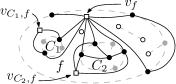
Figure 4: Graph (dashed lines; preassigned vertices are empty) and its connectivity assignment graph (solid lines, dummy vertices as boxes).

If a face $f$ is incident to a single connected component, we use for $E_{f}^{\prime}$ the ordinary assignment graph; the connectivity condition is trivial in this case. Now let $f$ be a face with $z_{f}>1$ incident connected components. For each component $C$ incident to $f$ that does not contain a vertex that is preassigned to $f$, we add a dummy vertex $v_{C,f}$ with demand 1 and connect it to all degree-2 vertices of $C$ incident to $f$; this ensures connectivity condition (1). Let $c_{f}$ denote the number of these dummy vertices, and note that there are exactly $c_{f}$ valencies assigned to $f$ due to these dummy vertices. Let $\widetilde{a}_{f}$ denote the number of free valencies assigned by $\widetilde{A}$, and let $\widetilde{d}_{f}$ denote the number of valencies a maximum indicator set in $f$ with respect to $\widetilde{A}$ misses. To ensure that the necessary valencies for the matching condition are present, we need that at least $\widetilde{d}_{f}-c_{f}$ vertices of $V_{b}$ are assigned to $f$. For connectivity condition (2) we need at least $2z_{f}-2-\widetilde{a}_{f}-c_{f}$ such vertices assigned to $f$. We thus create a dummy vertex $v_{f}$ whose demand is set to $s_{f}=\max\{2z_{f}-2-\widetilde{a}_{f}-c_{f},\widetilde{d}_{f}-c_{f},0\}$, possibly increasing this demand by 1 to guarantee the parity condition. Finally, we wish to allow an arbitrary even number of vertices in $V_{b}$ to be assigned to $f$. Since some valencies are already taken by dummy vertices, we do not just add to $E_{f}^{\prime}$ edges between non-adjacent vertices of $V_{b}$ incident to $f$ but for all such pairs. The valencies assigned by $\widetilde{A}$ and the dummy vertices satisfy the demand of any indicator set. Fig. 4 shows an example; for clarity edges connecting vertices in $V_{b}$ are omitted in $f$ and the outer face.

Lemma 8.

A perfect matching of $G_{A}^{\prime}$ (together with $\widetilde{A}$) corresponds to a node assignment that satisfies parity, matching, and connectivity condition for all faces, and vice versa.

Proof.

Let $M$ be a perfect matching of $G_{A}^{\prime}$ and let $A$ denote the corresponding node assignment. Let $f$ be a face of $G$, we show that $A$ satisfies the parity condition, the matching condition, and the parity condition for $f$. If $z_{f}=1$, the connectivity condition holds trivially and the remaining conditions follow from Theorem 2 since $M\cap E_{f}$ is a realization of $A$ for $f$. Hence, let $z_{f}\geq 2$.

Using the definition from above, there are $\widetilde{a}_{f}$ valencies assigned to $f$ by $\widetilde{A}$, $c_{f}$ valencies from vertices adjacent to the dummy vertices $v_{C,f}$, $s_{f}$ valencies from vertices incident to the dummy vertex $v_{f}$ and $2k_{f}$ valencies from $k_{f}$ edges in $M\cap\binom{X_{f}}{2}$. In total this are $\widetilde{a}_{f}+c_{f}+s_{f}+2k_{f}$ valencies, which is even due to the choice of $s_{f}$, and hence the parity condition holds.

For the connectivity condition, observe that the dummy vertices $v_{C,f}$ imply connectivity condition (1) and the choice of $s_{f}$ implies connectivity condition (2).

It remains to prove that the matching condition is satisfied. Let $T$ denote an indicator set of $f$ (for $A$). Observe that the vertices of an indicator set are either all in $V_{\mathrm{in}}$ or all in $V_{b}$. If $T\subseteq V_{\mathrm{in}}$, then $T$ was already an indicator set for $\widetilde{A}$, and its demand is satisfied due to the choice of $s_{f}$. If $T\subseteq V_{b}$, it is a joker, a pair, or a 3-cycle. However, as argued before, a 3-cycle can be excluded as it is either contained in $V_{\mathrm{in}}$ or one of its vertices must be matched to a dummy vertex in another face, and hence is not assigned to $f$. For a joker the necessary valency exists due to the parity condition. If $T$ is a pair (consisting of two adjacent vertices of degree 2), its vertices are contained in the same connected component. Since $z_{f}\geq 2$ and connectivity condition (1) is satisfied, at least one more vertex must be assigned to $f$. It then follows from the parity condition, that the demand of $T$ is satisfied. Thus the matching condition holds, finishing this direction of the proof.

Conversely, let $A$ be a node assignment that satisfies for each face $f$ the parity condition, the matching condition, and the connectivity condition. We construct for each face $f$ a matching $M_{f}\subseteq E_{f}$ satisfying exactly the demands of all vertices assigned to $f$ and the dummy vertices associated with $f$. Clearly the matching $M=\bigcup_{f\in\mathcal{F}}M_{f}$, where $\mathcal{F}$ denote the set of faces of $G$, then satisfies the demands of all vertices in $G_{A}^{\prime}$, that is it is a perfect matching of $G_{A}^{\prime}$.

Let $f$ be a face. If $z_{f}=1$, we choose $M_{f}$ as an arbitrary realization of $A$ for $f$, which exists by Theorem 2, and the condition is satisfied by construction. Hence assume $z_{f}\geq 2$. Connectivity condition (1) implies that each connected component either contains a vertex in $V_{\mathrm{in}}$ or a vertex in $V_{b}$ assigned to $f$. We pick for each connected component $C$ that does not contain a vertex in $V_{\mathrm{in}}$ an arbitrary assigned vertex of $V_{b}$ and match it to $v_{C,f}$. The matching condition implies that the number $r$ of remaining vertices in $V_{b}$ assigned to $f$ is at least $\widetilde{d}_{f}-c_{f}$, and connectivity condition (2) implies that $r$ is at least $2z_{f}-2-\widetilde{a}_{f}-c_{f}$. Thus, we can match arbitrary $s_{f}$ vertices in $V_{b}$ to $v_{f}$, satisfying its demand. The remaining yet-unmatched vertices assigned to $f$ are an even number and an arbitrary pairing of them completes the matching $M_{f}$. ∎

Together with the previous observations this directly implies an algorithm for finding connected 3-regular augmentations.

Theorem 8.

Connected FERA can be solved in $O(n^{2.5})$ time.

4.2 Biconnected FERA

In this section we show that also biconnected FERA can be solved efficiently. Again, we first give a local characterization of node assignments admitting biconnected augmentations and then construct a biconnectivity assignment graph whose perfect matchings correspond to such node assignments.

Local characterization of biconnectivity.

Let $G=(V,E)$ be a planar graph with a fixed embedding and let $f$ be a face of $G$. We consider the bridge forest $B_{f}$ of $f$, which is constructed as follows. Remove all bridges from $G$ and consider the connected components of this graph that are incident to $f$. We create a node for each such connected component and connect them by an edge if and only if they are connected by a bridge in $G$. Similarly, we can define the bridge forest of $f$ with respect to an augmentation $W$, where we only remove bridges of $G+W$. Observe that each leaf component in a bridge forest with respect to $W$ contains a subgraph that corresponds to a leaf component in the associated bridge forest of $G$. Clearly, an augmentation is connected if and only if the bridge graph of each face is connected, and it is biconnected if and only if each bridge forest consists of a single node. Observe that the bridge forest $B_{f}$ contains a connected component for each connected component of $G$ incident to $f$. We say that such a component is trivial if its corresponding connected component in $B_{f}$ consists of a single node. A 2-edge connected component of $G$ incident to $f$ is a leaf component if its corresponding node in $B_{f}$ has degree 1. Figure 5 shows an example.

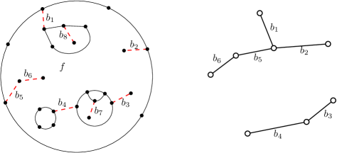
Figure 5: A face $f$ (right) and its corresponding bridge forest $B_{f}$ (right); bridges are dashed, red edges. The bridges $b_{7}$ and $b_{8}$ are not incident to $f$ and hence not contained in $B_{f}$.

Next, we study necessary and sufficient conditions for when a node assignment $A$ admits for a face $f$ a planar 3-regular augmentation $W_{f}$ such that the resulting bridge forest is a single node. Obviously, if there is more than one connected component incident to $f$, each of them must assign at least two valencies to $f$; if none is assigned, the augmentation will not be connected, if only one is assigned the single edge incident to this valency will form a bridge. Additionally, each leaf component must assign at least one valency, otherwise its incident bridge in $B_{f}$ will remain a bridge after the augmentation. Thus the following biconnectivity condition is necessary for a face $f$ with $z_{f}$ incident connected components to admit a biconnected augmentation.

Condition 5 (Biconnectivity condition).

1. If $z_{f}>1$, each connected component incident to $f$ must have at least two valencies assigned to $f$, and

2. each leaf component of $f$ must assign at least one valency to $f$.

We show that these conditions are also sufficient, both in the planar and in the non-planar case.

Theorem 9.

Let $G$ be a planar maxdeg-3 graph on $n$ vertices with a fixed embedding, and let $A$ be a node assignment. Then the following statements hold.

1. $A$ admits a biconnected realization if and only if $A$ satisfies the parity condition, the matching condition, and the biconnectivity condition for all faces of $G$.

2. The realization can be chosen to be planar if and only if $A$ additionally satisfies the planarity condition for faces of $G$. A corresponding realization for $A$ can be computed in $O(n)$ time.

Proof.

Clearly the conditions for both statements are necessary. We prove that they are also sufficient. Let $A$ be a node assignment satisfying the parity condition, the matching condition, and the biconnectivity condition for all faces of $G$. We construct a biconnected realization of $A$ for each face $f$; together they form a biconnected realization of $A$.

First assume that the bridge graph $B_{f}$ of $f$ is connected, that is $G$ has only one connected component incident to $f$. Let $W_{f}$ be a realization of $A$ for $f$ and assume that it is not a biconnected realization. Then there exists a bridge $b$ in $G+W_{f}$ whose endpoints are incident to $f$ in $G$. Without loss of generality we assume $b$ such that it is incident to a leaf of the bridge forest $B_{f}$ with respect to $W_{f}$. Consider the subtrees of $B_{f}$ on distinct sides of $b$. Each of them contains a leaf, and thus a vertex assigned to $f$. Let $x_{1},x_{2}$ denote two such vertices on distinct sides of $b$, choosing $x_{1}$ and $x_{2}$ as endpoints of $b$ if possible, and let $e_{1}=x_{1}y_{1}$ and $e_{2}=x_{2}y_{2}$ denote two edges of $W_{f}$ incident to $x_{1}$ and $x_{2}$, respectively. Since $b$ is a bridge in $G+W_{f}$, we have that $x_{1},x_{2},y_{1}$ and $y_{2}$ are pairwise disjoint, and except for possibly $x_{1}$ and $x_{2}$, which might be joined by $b$, they are pairwise non-adjacent. It is then not hard to see that replacing in $W_{f}$ the edges $x_{1}y_{1}$ and $x_{2}y_{2}$ by $x_{1}y_{2}$ and $x_{2}y_{1}$ yields a new augmentation $W_{f}^{\prime}$ of $G$ whose bridge forest has fewer leaves. Applying this construction iteratively yields a biconnected realization. Now assume that the bridge graph of $f$ is not connected and consists of $z_{f}$ connected components. By correctness of Rule 1, we may first add a set $W_{f}^{\prime\prime}$ of $z_{f}-1$ edges such that $G$ becomes connected. Observe that $G+W_{f}^{\prime\prime}$ is still a planar graph and contains the face $f$. Consider the assignment $A^{\prime}$ induced by $A$ on $G+W_{f}^{\prime\prime}$. The bridge forest $B_{f}^{\prime}$ of $G+W_{f}^{\prime\prime}$ for $f$ is connected, and each leaf component of $G+W_{f}^{\prime\prime}$ either is a connected component of $G$, or was already a leaf component in $G$. In both cases it follows that the leaf component contains at least one vertex assigned to $f$, which is incident to an edge from $W_{f}^{\prime\prime}$ that is not a bridge. Hence the construction also works for the case that $B_{f}$ is not yet connected, finishing the proof of claim (i).

For claim (ii) observe that by the same argument (applying Rule 2) instead of Rule 1), we may again assume that $B_{f}$ is connected. Now let $W_{f}$ be any planar realization of $A$ for a face $f$ of $G$ and let $b$ be a bridge that is incident to a leaf of $B_{f}$ (with respect to $W_{f}$). We again choose vertices $x_{1},x_{2},y_{1},y_{2}$ for rewiring, but slightly more carefully. Namely observe that in $G+W_{f}$ the bridge $b$ is incident to a face $f^{\prime}$ in $G+W_{f}$, and by the same argument as above this face must be bounded by at least two edges $x_{1}y_{1}$ and $x_{2}y_{2}$ of $W_{f}$, having their endpoints on distinct sides of $b$. We assume that the clockwise order of occurrence along the boundary of $f^{\prime}$ is $x_{1}x_{2}y_{2}y_{1}$. If $x_{1}$ and $x_{2}$ are not adjacent, we replace $x_{1}y_{1}$ and $x_{2}y_{2}$ by the two edges $x_{1}x_{2}$ and $y_{1}y_{2}$, which clearly is planar. If $x_{1}$ and $x_{2}$ are adjacent, that is $b=x_{1}x_{2}$, we replace them by $y_{2}x_{1}$ and $x_{2}y_{1}$, which is again planar since $b$ is incident to $f^{\prime}$ on both sides; see Fig. 6. As above it can be seen that the bridge graph of $G+W_{f}$ has fewer leaves, and thus iteratively applying the rewiring step yields the desired realization.

Figure 6: Illustration of the rewiring step from the proof of Theorem 9; $x_{1},x_{2}$ are not adjacent (left), and $x_{1},x_{2}$ are adjacent (right). The dashed black edges are part of an augmentation and are replaced by the dashed red edges. Afterwards the edge $b$ is not a bridge anymore.

Concerning the running time, recall that, by applying Rule 2, $z_{f}-1$ edges can be added to each face in $G$ in $O(n)$ time such that $G$ becomes connected. A planar (possibly not biconnected) realization $W_{f}$ of $A$ for each face $f$ in the connected graph $G$ can be computed in linear time by Theorem 6. For the rewiring we apply a right-first search along the boundary of $f$ handling the bridges that are incident to leaves of the bridge forest consecutively.

We start from a vertex outside a leaf component and search for the first bridge $b$ that is incident to a leaf component of $B_{f}$ (with respect to $W_{f}$). After crossing $b$ in the direction of the leaf, we follow the boundary of the face $f^{\prime}$ in $G+W_{f}$ that is incident to $b$ on both sides (instead of the boundary of $f$ in $G$). We store an edge $y_{1}x_{1}\in W_{f}$ at the leaf component (which exists by the arguments above) and the first edge $x_{2}y_{2}\in W_{f}$ on the other side of $b$, i.e., after crossing the bridge the second time. These edges are then rewired. If $x_{2}y_{2}$ was an edge in a leaf component before, there are no further bridges connected to the boundary of $f$ between $x_{2}$ to $y_{2}$ and we continue the search for the next bridge that is incident to a leaf from $y_{2}$, now again along the boundary of $f$. Otherwise, we recursively search for the next bridge starting from $x_{2}$ along the boundary of $f$, and apply the rewiring. When we reach $y_{2}$ again, the previously rewired edge incident to $y_{2}$ might be rewired again, however, at this point all bridges between $x_{2}$ and $y_{2}$ are remedied. The search continues at $y_{2}$ and finally stops at $y_{1}$ at the latest. Then $B_{f}$ consists of a single node. Hence, this search and the rewiring can be done in linear time with respect to the number of vertices incident to $f$. ∎

Next, we extend Theorem 3 to this setting, allowing us to additionally enforce the planarity condition for an assignment already satisfying the parity condition, the matching condition and the biconnectivity condition. Similar to the proof of Corollary 1, it can be seen that the rewiring performed in the proof of Theorem 3 does not invalidate the biconnectivity condition. It reassigns vertices to other faces only if a face is assigned an insufficient number of additional valencies, which only shortens long paths of degree-2 vertices but never reduces the number of assigned valencies of a leaf component to zero or of a connected component below two. We thus have the following corollary.

Corollary 2.

Let $G$ be a planar maxdeg-3 graph with a fixed embedding and let $A$ be a node assignment satisfying the parity condition, the matching condition, and the biconnectivity condition. Then a modified assignment $A^{\prime}$ that additionally satisfies the planarity condition can be computed from $A$ in $O(n)$ time.

The biconnectivity assignment graph.

We now show how to test efficiently whether such an augmentation exists. The idea is, as in the connected case, to consider a corresponding biconnectivity assignment graph that models the additional requirements. Let $G=(V,E)$ be a planar maxdeg-3 graph with a fixed embedding. We construct the biconnectivity assignment graph $G_{A}^{\prime\prime}$ of $G$ using similar techniques as for the connectivity assignment graph. In particular, we again consider the partition of the vertices of $V^{\tiny\leavevmode\hbox to4.37pt{\vbox to4.37pt{\text{[drawing]}}}}$ into the sets $V_{\mathrm{in}}$ with a fixed assignment and $V_{b}$ that may be assigned to two different faces, and the corresponding preliminary assignment $\widetilde{A}$. We note that unlike in the connectivity case, a graph that contains a non-empty triangle generally does not admit a biconnected augmentation as one of the edges incident to such a triangle necessarily forms a bridge. Hence if $G$ admits a biconnected 3-regular augmentation, all triangles are empty, and thus assigned by $\widetilde{A}$.

Again the biconnectivity assignment graph $G_{A}^{\prime\prime}=(V^{\prime\prime},E^{\prime\prime})$ is formed on a superset $V^{\prime\prime}\supseteq V_{b}$ of the vertices without a fixed assignment. We now describe an edge set $E_{f}$ for each face $f$. As before, the final interpretation will be that in the assignment induced by a (generalized) perfect matching $M$ of $G_{A}^{\prime\prime}$ a vertex $v\in V_{b}$ is assigned to $f$ if and only if it is incident to an edge in $M\cap E_{f}$. If a face $f$ is incident to a single connected component whose bridge forest consists of a single node, we use the ordinary assignment graph, where $E_{f}$ consists of edges between all non-adjacent pairs of vertices from $V^{\tiny\leavevmode\hbox to4.37pt{\vbox to4.37pt{\text{[drawing]}}}}$ incident to $f$. Now assume that $f$ does not have this property. To enforce the biconnectivity condition, we consider the leaf components of $f$. For each leaf component $L$ that does not contain vertices preassigned to $f$, we add a dummy vertex $v_{L,f}$ with demand 1 and connect it to all vertices from $V_{b}$ of $L$ incident to $f$; this clearly enforces biconnectivity condition (2). Moreover, for each connected component of $f$ that contains a bridge this also enforces biconnectivity condition (1). If $G$ is not connected, we add for each connected component $C$ that neither contains a bridge nor any vertices preassigned to $f$, a dummy vertex $v_{C,f}$ with demand 2 and connect it to all vertices of $C$ that are in $V_{b}$ and incident to $f$. Note that these components are no leafes by definition. Let $c_{f}$ denote the number of valencies demanded by dummy vertices $v_{C,f}$ and $\ell_{f}$ the number of valencies demanded by dummy vertices $v_{L,f}$. We compute the demand $\widetilde{d}_{f}$ of the preassigned vertices as in the construction of the connectivity assignment graph. To satisfy this demand, at least $\widetilde{d}_{f}-c_{f}-\ell_{f}$ additional vertices from $V_{b}$ need to be assigned to $f$. We thus set $n_{f}=\max\{\widetilde{d}_{f}-c_{f}-\ell_{f},0\}$. To ensure this and the parity condition, we add a new dummy vertex $v_{f}$ with demand $s_{f}$, where $s_{f}=n_{f}$ if $n_{f}+\widetilde{a}_{f}+c_{f}+\ell_{f}$ is even and $s_{f}=n_{f}+1$, otherwise. Finally, we allow an arbitrary even number of vertices of $V_{b}$ incident to $f$ to be matched by adding to $E_{f}$ all edges in $\binom{X_{f}}{2}$, where $X_{f}$ denotes the vertices in $V_{b}$ incident to $f$. The connectivity assignment graph in Figure 4 coincides with the biconnectivity assignment graph for the given graph, except for the demands of $v_{C_{1},f}$ and $v_{C_{2},f}$. They are set to 2 here, because the corresponding components neither contain a bridge nor any preassigned vertices. Recall that, for reasons of clarity, the edges between vertices of $V_{b}$ incident to the face $f$ are omitted.

Lemma 9.

Let $G$ be a maxdeg-3 graph with a fixed embedding and let $G_{A}^{\prime\prime}$ be its biconnectivity assignment graph. Then each perfect matching $M$ of $G_{A}^{\prime\prime}$ induces (together with the preliminary assignment $\widetilde{A}$) a node assignment that satisfies for each face the parity condition, the matching condition, and the biconnectivity condition. Conversely, for each such node assignment $A$ there exists a perfect matching $M$ of $G_{A}^{\prime}$ that induces it.

Proof.

Let $M$ be a perfect matching and let $A$ be the corresponding node assignment. For faces $f$ that are incident to a single connected component whose bridge graph consists of a single node, $E_{f}$ is chosen as in the ordinary assignment graph, and thus $A$ satisfies the parity condition and the matching condition for $f$. The biconnectivity condition holds trivially for these faces. Now assume that $f$ is a face not having this property. Clearly, the demand of $s_{f}$ ensures that an even number of valencies is assigned to $f$, and hence $A$ satisfies the parity condition. Moreover, the dummy vertices $v_{C,f}$ and $v_{L,f}$ explicity ensure the biconnectivity condition. For the matching condition, recall that $s_{f}$ was chosen such that the demands of all matching indicator sets consisting of vertices in $V_{\mathrm{in}}$ are satisfied. Thus, if there is a matching indicator set whose demand is not satisfied, it would consist of vertices in $V_{b}$, and hence would be a joker, a pair or a 3-cycle. Let $T$ be such an indicator set. That the demands of jokers and pairs are satisfied can be argued as in Lemma 8. If $T$ is a 3-cycle, it forms a non-empty triangle (as it would be preassigned otherwise), but then, as argued above, a biconnected augmentation does not exists. Hence this case cannot occur, and the matching condition is satisfied.

Conversely let $A$ be a node assignment satisfying the parity condition, the matching condition, and the biconnectivity condition. We construct for each face $f$ a matching $M_{f}\subseteq E_{f}$ satisfying exactly the demands of all vertices assigned to $f$ and the dummy vertices associated with $f$. If $f$ is incident to a single connected component of $G$, and the bridge forest of this component is a single node, a realization of $A$ for $f$, which exists by Theorem 9, forms the desired matching. Otherwise, the conditions satisfied by $A$ imply that we can find enough vertices of $V_{b}$ assigned to $f$ and match them to the dummy vertices associated with $f$. The choice of their demands and the parity condition imply that the number of unmatched vertices in $V_{b}$ assigned to $f$ is even, and they can be paired arbitrarily in $G_{A}^{\prime\prime}$ to form $M_{f}$. ∎

To decide biconnected FERA for a given maxdeg-3 graph on $n$ vertices with a fixed embedding, we thus first construct in $O(n^{2})$ time the biconnectivity assignment graph $G_{A}^{\prime\prime}$ and compute in $O(n^{2.5})$ time a perfect (generalized) matching in it. If such a matching does not exist, then a biconnected augmentation does not exist by Theorem 9 (i). Otherwise, such a matching induces a node assignment satisfying the parity condition, the matching condition, and the biconnectivity condition by Lemma 9. Using Corollary 2, we modify it in $O(n)$ time to a node assignment additionally satisfying the planarity condition. A corresponding augmentation can then be found in $O(n^{2})$ time by Theorem 9(ii).

Theorem 10.

Biconnected FERA can be solved in $O(n^{2.5})$ time.

5 Proof of Completeness of Triconnected FERA

Theorem 11.

Triconnected FERA is NP-complete, even if the input graph is already biconnected.

Proof.

Triconnected FERA is in $NP$ since, given a planar graph $G$ with a fixed embedding, we can guess a set $W\subseteq\binom{V}{2}$ of non-edges of $G$ and then test efficiently whether the graph $G+W$ is 3-regular, planar, and triconnected, and that $W$ respects the given embedding of $G$ (the latter can be checked using an algorithm due to Angelini et al. [adfjk-tppeg-10]). We prove NP-hardness by reducing from the problem MonotonePlanar3Sat, which is known to be NP-hard [bk-obsp-10]. It is a special variant of Planar3Sat, which we use in the next section for the hardness proof of PRA.

Figure 7: Layout of a (monotone) planar 3Sat formula.

A monotone planar 3Sat formula is a 3Sat formula whose clauses either contain only positive or negative literals and whose variable–clause graph is planar. A monotone rectilinear representation of a monotone planar 3Sat formula is a drawing of the variable–clause graph such that the variables correspond to axis-aligned rectangles on the x-axis and clauses correspond to non-crossing three-legged “combs” above the x-axis if they contain positive variables and below the x-axis otherwise; see Fig. 7. An instance of MonotonePlanar3Sat is a monotone rectilinear representation of a monotone planar 3Sat formula $\varphi$. We now construct a biconnected graph $G_{\varphi}$ with a fixed planar embedding that admits a planar 3-regular triconnected augmentation if and only if $\varphi$ is satisfiable.

The graph $G_{\varphi}$ consists of so-called gadgets, that is subgaphs that represent the variables, literals, and clauses of $\varphi$; see Fig. 8. For each gadget, we will argue that there are only a few ways to augment it to be 3-regular, triconnected and planar. Note that our construction connects variable gadgets corresponding to neighboring variables in the layout of the variable–clause graph of $\varphi$. Hence $G_{\varphi}$ is always connected. Additionally, we identify the left boundary of the leftmost variable gadget with the right boundary of the rightmost variable gadget. In the figure vertices with degree less than 3 are highlighted by white disks. All bends and junctions of line segments represent vertices of degree at least 3. Vertices of degree greater than 3 are actually modeled by small cycles of vertices of degree 3, as indicated in the left of Fig. 8. The (black thick and thin) solid line segments between adjacent vertices represent the edges of $G_{\varphi}$; the dotted line segments represent non-edges of $G_{\varphi}$ that are candidates for an augmentation of $G_{\varphi}$. Gaps in the thick black line segments of the literal gadgets indicate positions where further subgraphs can be plugged in depending on the number of clauses containing the literal.

Each variable gadget consist of two symmetric parts, which correspond to the two literals. These literal (sub)gadgets are separated by (thick) horizontal edges. The degree-2 vertex $u$ is incident to both literal gadgets. The thin triangle at the right side is called the parity triangle (see Fig. 8). Each literal gadget contains a subgraph that is attached to the horizontal edges separating the literals in only two vertices, which thus form a separator of size 2. We call this subgraph the literal body. The literal body can be considered as a path of smaller (thin) subgraphs connected by thick black edges. The thin subgraphs can be characterized as a triangle at the front side (front triangle) that is based on another triangular shaped subgraph (triangle basement) and further oppositely placed pairs of triangles. In Fig. 8 we exemplarily marked a front triangle with its triangle basement and a pair of triangles. In the construction the number of pairs of triangles in the literal body corresponds to the number of clauses containing the literal. Note that w.l.o.g. we may assume that each literal appears in at least one clause. The necessary number of pairs of triangles can be plugged in at the gap. The corresponding clauses are attached to the outer boundary of the literal gadget, as exemplarily shown in Fig. 8. Each attached clause thereby induces a pair of adjacent degree-2 vertices at the boundary that are incident to the literal gadget and to the clause gadget. We call the corresponding valencies the boundary valencies of the literal gadget. Thus, each literal gadget has twice as many boundary valencies as clauses contain the literal.

Consider the graph $G_{\varphi}^{\prime}$ that we obtain by deleting the literal bodies, contracting the parity triangles and ignoring degree-2 vertices. We claim that $G_{\varphi}^{\prime}$ is 3-vertex connected. This is true since (a) the subgraph of $G_{\varphi}^{\prime}$ induced by the variable gadgets is 3-connected and (b) each subgraph induced by a clause gadget is also 3-connected and is attached to the former (variable gadget) subgraph in twelve vertices. Hence, a 3-regular triconnected augmentation of $G_{\varphi}$ only needs to care for the connectivity at the literal bodies and the parity triangles. Note that $G_{\varphi}$ is already biconnected since it is obtained from a 3-connected graph by subdividing edges, replacing degree-2 vertices by (parity) triangles and adding paths of biconnected subgraphs (literal bodies) between existing endpoints. In the following we call a 3-regular, triconnected, planar augmentation a valid augmentation. We show two properties of $G_{\varphi}$:

1. Let $W$ denote a valid augmentation and $x$ a variable gadget. Then for at least one literal gadget in $x$ the augmentation $W$ assigns all boundary valencies to the incident literal face.

2. Given a literal $L$ and a (sub)set of clauses containing $L$, there exists a valid augmentation of the corresponding variable gadget that uses all boundary valencies of $L$ apart from those that are incident to the given clauses.

Figure 8: Variable gadget for variable $x$ and clause gadget for clause $(y\vee x\vee z)$ in graph $G_{\varphi}$. The augmentation (dotted edges) corresponds to the assignment $x=$ture, $\neg x=$false.

We start with (P1). Consider the exemplary variable gadget in Fig. 8. The valency of $u$ is incident to both literal (sub)gadgets, and hence, is either assigned to $x$ or $\neg x$ by a valid augmentation. Without loss of generality, assume that $u$ is assigned to $x$. The opposite case is symmetric. The two degree-2 vertices in the triangle basement in $\neg x$ are thus connected since the inner face of the literal body provides no further valencies. Let $\ell$ denote the number of clauses containing $\neg x$. The outer face of the literal body of $\neg x$ is incident to $2(\ell+1)$ valencies; $\ell+1$ stem from the triangles at the literal body, $\ell$ are boundary valencies and one additional valency is placed at the triangle to the right. We argue that the valencies at the triangles of the literal body are not connected to each other by a valid augmentation. This is true since such an edge would immediately induce a subgraph that is separated from the rest by only two vertices; namely the vertices where the connected triangles are attached to the literal body. Consequently, a valid augmentation must assign all $\ell$ boundary valencies of $\neg x$ to the literal face. The last valency, which is necessary due to the parity condition, is provided by the vertex at the thick triangle to the right.

For the proof of (P2) consider again Fig. 8 and let (without loss of generality) $x$ denote the given literal. The number of clauses containing $x$ is $\ell$, $0\leq s\leq\ell$ denotes the cardinality of the given subset of the clauses containing $x$. In order to construct a valid augmentation $W$ of the variable gadget such that $W$ uses exactly $2(\ell-s)$ boundary valencies of $x$, we connect $u$ to a valency in $x$. This induces an augmentation of $\neg x$ as described in the proof of (P1). Note that this augmentation makes the triangle basement in $\neg x$ triconnected and all the triangles of the literal body are connected to vertices outside the literal body, which also makes the literal body triconnected. In the literal gadget for $x$ the only vertex that can be connected to $u$ belongs to the triangle basement. Hence, the two remaining degree-2 vertices at the front side of the literal body are also connected. Furthermore, we connect the valency at the parity triangle to the only possible vertex at the opposite thick edge, which makes the parity triangle triconnected. Finally, we choose the $s$ upper pairs of triangles at the literal body and connect each by an edge. In contrast to the proof of (P1) connecting opposite triangles at the literal body is feasible, since the new edge incident to $u$ ensures triconnectivity. The remaining $2(\ell-s)$ valencies at the literal body can be obviously connected in a planar way to the $2(\ell-s)$ boundary valencies that are not incident to the given clauses, which finally ensures the triconnectivity of the whole augmented variable gadget.

With the help of (P1) and (P2) it is now easy to show that if $G_{\varphi}$ admits a valid augmentation then $\varphi$ is satisfiable. Assume that $W$ is a valid augmentation. Then $W$ connects the two degree-2 vertices of each clause to two boundary valencies of literal gadgets since connecting those degree 2 to each other would yield a parallel edge. This selects a set of literal gadgets in that sense that a gadget is selected if at least one of its boundary valencies is assigned to a clause face. According to (P1) the boundary valencies of the negated literal gadget of a selected gadget are all assigned to the literal face, and hence, a literal and its negation are never selected at the same time. Thus, the literal selection induces a truth assignment of the variables, which satisfies $\varphi$ since each clause selects at least one (true) literal.

Conversely, we need to show that if $\varphi$ is satisfiable then $G_{\varphi}$ admits a valid augmentation. Assume we have a satisfying truth assignment for $\varphi$. For each clause, we choose exactly one true literal $L$ and connect the two degree-2 vertices of the clause to the two boundary valencies of $L$ that are incident to the clause gadget. This ensures triconnectivity at the former degree-2 vertices of the clause and the former degree-2 vertices providing the boundary valencies, and thus, yields a valid augmentation of the clause gadgets. Recall that $G^{\prime}_{\varphi}$ is already triconnected. With the help of (P2) this can be finally extended to a valid augmentation of $G_{\varphi}$. ∎

6 Proof of Completeness of PRA

Theorem 1. PRA is NP-complete, even if the input graph is biconnected.

Proof.

PRA is in $NP$ since given a planar graph $G$ we can guess a set $W\subseteq\binom{V}{2}$ of non-edges of $G$ and then test efficiently whether $G+W$ is 3-regular and planar. We prove NP-hardness by reducing from the problem Planar3Sat, which is known to be NP-hard [l-pfu-82]. The reduction is inspired by and indeed very similar to a reduction of Rutter and Wolff [rw-acpgg-12], showing that it is NP-hard to find a smallest edge set that augments a given graph to be 2-edge connected and planar.

An instance of Planar3Sat is a 3Sat formula $\varphi$ whose variable–clause graph is planar. Such a graph can be laid out (in polynomial time) such that the variables correspond to pairwise axis-aligned rectangles on the x-axis and clauses correspond to non-crossing three-legged “combs” above or below the x-axis [kr-pcr-92]; see Fig. 7. We now construct a biconnected planar graph $G_{\varphi}$ that admits a planar 3-regular augmentation if and only if $\varphi$ has a satisfying truth assignment.

Figure 9: Part of the graph $G_{\varphi}$ for a SAT formula $\varphi$ that contains the clause $(x\vee\neg y\vee z)$. The augmentation (dotted edges) corresponds to the assignment $x=y=$false and $z=$true.

The graph $G_{\varphi}$ again consists of gadgets, which are subgaphs that represent the variables, literals, and clauses of $\varphi$; see Fig. 9. For each gadget, we will argue that there are only a few ways to embed and augment it to be 3-regular and planar. Note that our construction connects variable gadgets corresponding to neighboring variables in the layout of the variable–clause graph of $\varphi$. Hence $G_{\varphi}$ is always connected. Additionally, we identify the left boundary of the leftmost variable gadget with the right boundary of the rightmost variable gadget. In the figure vertices with degree less than 3 are highlighted by small black disks. All bends and junctions of line segments represent vertices of degree at least 3. Vertices of degree greater than 3 are actually modeled by small cycles of vertices of degree 3, as indicated in the left of Fig. 9. The (black and dark gray) solid line segments between adjacent vertices represent the edges of $G_{\varphi}$; the thick dotted line segments represent non-edges of $G_{\varphi}$ that are candidates for an augmentation of $G_{\varphi}$. The set of solid black edges forms a subgraph of $G_{\varphi}$ that we call the frame. The dark gray solid edges form free chains, which connect two degree-2 vertices to the frame. Consider the graph $G_{\varphi}^{\prime}$ that is obtained from the frame by contracting all vertices of degree 2 and all cycles that are used to model vertices of degree greater than 3. The graph $G_{\varphi}^{\prime}$ coincides with the one used by Rutter and Wolff in their reduction [rw-acpgg-12], and they show that it is 3-connected, and thus has a unique planar embedding [w-cgcg-32].

Since subdividing edges and replacing a vertex of degree at least 4 by a cycle preserves 3-connectedness, the frame has a unique embedding as well. In other words, the embedding of $G_{\varphi}$ is fixed up to embedding the free chains, which may be embedded in two distinct faces, each.

A 3-regular planar augmentation of $G_{\varphi}$ yields an embedding of $G_{\varphi}$ and an assignment of the degree-2 vertices of $G_{\varphi}$ to incident faces (a vertex $v$ is assigned to the face $f$ if in the planar embedding of $G+W$ the edge of $W$ incident to $v$ is embedded in the (former) face $f$) such that

1. each face is assigned an even number of vertices,

2. each face that is assigned two adjacent vertices is assigned at least four vertices.

We call such an assignment of degree-2 vertices to faces valid. Conversely, it is readily seen that given a valid assignment, a planar 3-regular augmentation can always be constructed. We thus need to show that if $G_{\varphi}$ admits an embedding with a valid assignment, then $\varphi$ is satisfiable.

Our variable gadget consists of two rows of square faces where the horizontal edge between the two leftmost faces and the horizontal edge between the two rightmost faces is missing. Effectively, the inner faces of a variable box form a cycle. Starting from the leftmost (rectangular) face, we call the faces odd and even. Each interior vertical edge is subdivided by a degree-2 vertex. Due to property (P1), these subdivision vertices must either all be assigned to the odd faces or all to the even faces of the variable. If the vertices are assigned to the even faces, then the corresponding variable is true, and vice versa.

A literal gadget consists of a square face that lies immediately above or below the variable gadget. A positive literal (such as the one labeled with $x$ in Fig. 9) is attached to an even face, a negated literal (such as the one labeled with $\neg y$ in Fig. 9) is attached to an odd face. A literal gadget contains two adjacent subdivision vertices at the edge it shares with the clause gadget, and a free chain containing two adjacent vertices of degree 2. The latter is attached to the boundary shared by the literal gadget with the variable gadget. Due to property (P2) the free chain must either be embedded inside the literal gadget and all incident degree-2 vertices are assigned to the face of the literal gadget, or the chain is embedded inside the attached variable gadget and the two subdivision vertices are assigned to the adjacent clause gadget. Again due to property (P2) the free chain must be embedded inside the literal gadget if no vertices are assigned to the adjacent face of the variable gadget. In this case the literal has the value false. If two vertices are assigned to the adjacent face of the variable gadget, the free chain can (but does not have to) be embedded inside the variable and the two subdivision vertices are assigned to the clause.

Finally, each clause gadget consists of a single rectangular face that contains two adjacent subdivision vertices. If $G_{\varphi}$ admits an embedding with a valid assignment, then, due to property (P2), at least two other degree-2 vertices are assigned to the clause gadget face. This means that for each clause gadget, the two subdivision vertices of at least one literal are assigned to the clause gadget. In other words, at least one of the literals that make up the clause is true. Hence, $\varphi$ has a satisfying truth assignment.

Conversely, it is easy to see that if $\varphi$ has a satisfying truth assignment, then an embedding with a corresponding assignment can be found. We use a constant number of vertices and edges for each literal and clause gadget, thus our reduction—including the computation of the embedding of the variable–clause graphs—is polynomial. Moreover, since the graph $G_{\varphi}$ is obtained from a 3-connected graph by subdividing edges and adding some paths between existing endpoints, the graph $G_{\varphi}$ is biconnected. ∎

7 Conclusion

In this paper we have given efficient algorithms for deciding whether a given planar graph with a fixed embedding admits a 3-regular planar augmentation. We note that the running time of $O(n^{2.5})$ is due to the potentially quadratic size of our assignment graphs. Recently, we succeeded in constructing equivalent assignment graphs with only $O(n)$ edges. This immediately improves the running time of all our algorithms to $O(n^{1.5})$.

References

[1]
M. Abellanas, A. García, F. Hurtado, J. Tejel, and J. Urrutia.
Augmenting the connectivity of geometric graphs.
Computational Geometry Theory and Applications, 40(3):220–230,
2008.
[2]
M. Al-Jubeh, M. Ishaque, K. Rédei, D. L. Souvaine, and C. D. Tóth.
Tri-edge-connectivity augmentation for planar straight line graphs.
In Yingfei Dong, Ding-Zhu Du, and Oscar H. Ibarra, editors, Proceedings of the 20th International Symposium on Algorithms and Computation
(ISAAC’09), volume 5878 of Lecture Notes in Computer Science, pages
902–912. Springer, 2009.
[3]
P. Angelini, G. Di Battista, F. Frati, V. Jelínek, J. Kratochvíl,
M. Patrignani, and I. Rutter.
Testing planarity of partially embedded graphs.
In Proceedings 21st ACM-SIAM Symposium on Discrete Algorithms
(SODA’10), pages 202–221. SIAM, 2010.
[4]
M. de Berg and A. Khosravi.
Optimal binary space partitions in the plane.
In Proc. 16th International Computing and Combinatorics
Conference (COCOON’2010), volume 6196 of LNCS, pages 216–225.
Springer, 2010.
[5]
G. A. Dirac.
Some theorems on abstract graphs.
Proceedings of the London Mathematical Society, s3-2:69–81,
1952.
[6]
K. P. Eswaran and R. E. Tarjan.
Augmentation problems.
SIAM Journal on Computing, 5(4):653–665, 1976.
[7]
H. N. Gabow.
An efficient reduction technique for degree-constrained subgraph and
bidirected network flow problems.
In Proceedings of the 15th annual ACM Symposium on Theory of
Computing (STOC’83), pages 448–456. ACM, 1983.
[8]
F. Hurtado and C. D. Tóth.
Plane geometric graph augmentation: a generic perspective.
In Thirty Essays on Geometric Graph Theory (J. Pach, ed.),
Algorithms and Combinatorics, 29, 2012.
[9]
G. Kant. and H. L. Bodlaender.
Planar graph augmentation problems.
In Proceedings of the 2nd Workshop Algorithms and Data
Structures (WADS’91), volume 519 of Lecture Notes in Computer Science,
pages 286–298. Springer, 1991.
[10]
D. E. Knuth and A. Raghunathan.
The problem of compatible representatives.
SIAM Journal on Discrete Mathematics, 5(3):422–427, 1992.
[11]
D. Lichtenstein.
Planar formulae and their uses.
SIAM Journal on Computing, 11(2):329–343, 1982.
[12]
H. Nagamochi and T. Ibaraki.
Graph connectivity and its augmentation: applications of ma
orderings.
Discrete Applied Mathematics, 1–3:447–472, 2002.
[13]
A. Pilz.
Augmentability to cubic graphs.
In Proceedings of the 28th European Workshop on Computational
Geometry (EuroCG’12), pages 29–32, 2012.
[14]
I. Rutter and A. Wolff.
Augmenting the connectivity of planar and geometric graphs.
Journal of Graph Algorithms and Applications, 16(2):599–628,
2012.
[15]
C. D. Tóth.
Connectivity augmentation in plane straight line graphs.
Electronic Notes in Discrete Mathematics, 31:49–52, 2008.
[16]
T. Watanabe and A. Nakamura.
Edge-connectivity augmentation problems.
Journal of Computer and System Sciences, 35(1):96–144, 1987.
[17]
H. Whitney.
Congruent graphs and the connectivity of graphs.
Amer. J. Math., 43:150–168, 1932.