Confining spheres within hyperspheres

Abstract

The bending energy of any freely deformable closed surface is quadratic in its curvature. In the absence of constraints, it will be minimized when the surface adopts the form of a round sphere. If the surface is confined within a hypersurface of smaller size, however, this spherical state becomes inaccessible. A framework is introduced to describe the equilibrium states of the confined surface. It is applied to a two-dimensional surface confined within a three-dimensional hypersphere of smaller radius. If the excess surface area is small, the equilibrium states are represented by harmonic deformations of a two-sphere: the ground state is described by a quadrupole; all higher multipoles are shown to be unstable.

$1$ Instituto de Ciencias Nucleares, Universidad Nacional Autónoma de México
Apdo. Postal 70-543, 04510 México, D.F., MEXICO
$2$ Departamento de Matemáticas Aplicadas y Sistemas,
Universidad Autónoma Metropolitana-Cuajimalpa, C.P. 01120, México D.F., MEXICO

PACS numbers: 45.10.Db, 02.40.-k, 87.16.D-

1 Introduction

Twenty five years ago, Nickerson and Manning examined how an elastic curve minimizes its energy when its freedom to bend in space is constrained by a two-dimensional obstacle [1, 2]. Their motivation was to understand the wrapping of DNA, a semi-flexible polymer, around histone cylinders but the question is also relevant to an understanding of the confinement of DNA within viral capsids (see, for example, [3]).

Whereas a space curve minimizes the Euclidean distance between two points by negotiating obstacles along surface geodesics, an elastic curve generally will not. This is because the relevant energy is not arc-length but the bending energy of the curve in three-dimensional space, quadratic in the spatial Frenet curvature $k$ [4]. This energy is always greater than its surface counterpart, quadratic in the geodesic curvature $\kappa_{g}$, characterising how the curve bends within the surface. By projecting the curvature vector of the space curve along the surface and normal to it, its bending energy can be decomposed as a sum of two contributions: $k^{2}=\kappa_{g}^{2}+\kappa_{n}^{2}$ [5]; whereas the intrinsic $\kappa_{g}$ is insensitive to the three-dimensional environment, the normal curvature $\kappa_{n}$ will register how the surface itself bends in space. When the surface is a sphere, $\kappa_{n}$ is a constant and thus the spatial bending energy will be minimized by surface geodesics. The snag, however, is that the boundary conditions, and in particular the closure of the curve, tend to be incompatible with geodesic behavior.

In [6] the equilibrium states of a closed elastic loop confined within a sphere were examined. It was found that, if the loop is short, there is a unique ground state; it is completely attached and it exhibits a two-fold dihedral symmetry, shown in Fig. 1. This state is stable; all of its excited counterparts are unstable. The bending energy was also found to depend–in a surprisingly sensitive way–on the length of the loop. Contradicting naive expectations, neither the energy nor the forces transmitted to the sphere increase monotonically with loop length. Local maxima are associated with the incommensurability of loop length with the equatorial circumference.

Figure 1: Equilibrium state of an elastic loop with two-fold symmetry

In this paper, higher dimensional analogues of a confined elastic loop will be examined. In particular, the focus will be on confined two-dimensional surfaces. The surface energy is now the two-dimensional bending energy, quadratic in its curvature (see, for example, [7, 8, 9, 10, 11, 12]). In the absence of constraints, it is simple to demonstrate that the closed surface minimizing this energy will be a round sphere.

The obvious higher-dimensional analogue of a confined loop is a two-dimensional closed surface confined within a sphere of smaller area. This is a problem of considerable interest from a biological perspective–where the morphology of cellular compartments may involves the confinement of one membrane within another–and it has been explored recently by Kahraman et al. [13, 14]. In distinction to the loop, which attaches everywhere to the sphere, the confined surface must detach somewhere, folding into the cavity. The interesting behavior occurs within these interior folds and along the boundaries of the regions of contact, not within the regions of contact themselves.

A more appropriate analogue of the confined loop is provided by locating the surface in a higher dimensional environment. The simplest possibility is to embed the two-dimensional surface in a four-dimensional Euclidean geometry, confining it within a three-dimensional hypersurface, and, in particular, a hypersphere of smaller radius. While this may appear a somewhat recondite exercise from the practical–application-driven–point of view of condensed matter, geometrically it is the natural generalization of the confined loop. Mathematically, it also can be viewed as a natural generalization of the Willmore problem involving competing length scales[7, 8]. Indeed, when the constraint on the area is relaxed, it reduces to the Willmore problem as formulated on a three-sphere, $\mathbb{S}^{3}$.

To address this problem, the constraint is imposed by introducing a local Lagrange multiplier. This generalizes the variational framework developed in [6]. The advantage of this approach is that the multiplier quantifies directly the loss of Euclidean invariance associated with the constraint; it becomes a source for the stress induced in the surface, its value at any point identified with the local normal force associated with the constraint.

If a surface of area greater than $4\pi$ is confined within a unit hypersphere it will generally buckle into a non-spherical shape. Unlike its loop counterpart, however, this problem is not tractable analytically. In this paper, it will be treated perturbatively in the regime where the surface area is marginally greater than $4\pi$. In analogy to a circular loop confined within a sphere, it is found that the confined equilibrium shapes are quantized. These states are represented by spherical harmonic deformations of a two-sphere. The ground state is a quadrupole, exhibiting a three-fold degeneracy; all higher multipoles turn out to be unstable.

The paper is organized as follows: In section 2, the variational framework is introduced. The Euler-Lagrange equations for the surface are derived and the constraining force identified. Whereas the local confining force typically is not constant, it will be if the confinement is within a hypersphere. In section 3 the weak confinement of a two dimensional sphere by a spherical hypersurface is examined. The paper concludes with a brief discussion and suggestions for future work in section 4. A number of useful definitions, identities and derivations are collected in a set of appendices.

2 Confining surfaces by hypersurfaces

Consider a surface $\Gamma_{N}$ of fixed area constrained to lie on a hypersurface $\Sigma_{N+1}$ in an $N+2$-dimensional Euclidean space [15]. The surface and hypersurface embeddings in Euclidean space are described parametrically by the maps $\Gamma_{N}:(s^{1},\cdots,s^{N})\rightarrow\mathbf{Y}(s^{1},\cdots,s^{N})$ and $\Sigma_{N+1}:(u^{1},\cdots,u^{N+1})\rightarrow\mathbf{X}(u^{1},\cdots,u^{N+1})$ respectively. The embedding of the surface on the hypersurface is described by a third mapping $\Gamma_{N,N+1}:(s^{1},\cdots,s^{N})\rightarrow(U^{1}(s^{1},\cdots,s^{N}),\cdots,U^{N+1}(s^{1},\cdots,s^{N}))$. The three mappings are related by composition, ${\bf Y}={\bf X}\circ U$. While the problem of specific interest will be in a two-dimensional surface embedded in a three-dimensional hypersphere, the dependence of the confinement process on the dimension as well as the confining geometry is not without interest and involves no significant additional calculational cost.

If the surface is freely deformable its bending energy is given by [10]

$$H=\frac{1}{2}\int dA_{N}\,(\nabla^{2}{\bf Y})^{2}\,,$$ (1)

where $\nabla^{2}$ is the Laplacian on $\Gamma_{N}$ and $A_{N}$ its area, both of which are constructed using the induced metric on $\Gamma_{N}$, $g_{ab}$, as described in the appendix.

In order to enforce the condition that $\Gamma_{N}$ lies on $\Sigma_{N+1}$, a term enforcing this constraint is added to the energy $H[\mathbf{Y}]$ given by Eq. (1):

$$H_{c}[\mathbf{Y},U]=H[\mathbf{Y}]+\int\,dA_{N}\,\,\bm{\lambda}(s)\cdot\left[\mathbf{Y}(s)-\mathbf{X}(U(s))\right]+\mu\left(\int dA_{N}-{\cal A}_{0}\right)\,,$$ (2)

which involves a vector-valued Lagrange multiplier $\bm{\lambda}$ defined along on $\Gamma_{N}$. This constraint will break the manifest translational invariance of the energy $H$. A second term enforces the constraint fixing the area. It involves a Lagrange multiplier $\mu$ which is constant.

The response of $H_{c}$ to a change $\mathbf{Y}\to{\bf Y}+\delta{\bf Y}$ in the embedding functions can be cast in the form

$$\delta_{\bf Y}H_{c}=\int dA_{N}\,\left(\nabla_{a}\mathbf{f}^{a}+{\bm{\lambda}}\right)\cdot\delta\mathbf{Y}\,,$$ (3)

where $\nabla_{a}$ is the covariant derivative on $\Gamma_{N}$ compatible with the induced metric $g_{ab}$ and the surface stress ${\bf f}^{a}$ is given by

$${\bf f}^{a}={\bf f}^{a}_{B}-\mu g^{ab}{\bf e}_{b}\,;$$ (4)

it involves a contribution associated with the bending energy given by [16]

$${\bf f}^{a}_{B}=K_{I}\left(K^{abI}-\frac{1}{2}g^{ab}K^{I}\right)\,{\bf e}_{b}-\tilde{\nabla}^{a}K_{I}\,{\bf n}^{I}\,,$$ (5)

as well as a tension associated with the constraint on the area. The simplest derivation of Eq. (3) involves a straightforward generalization of the method of auxiliary variables introduced in [17]. The details are provided in Appendix B. Here ${\bf e}_{a}=\partial{\bf Y}/\partial s^{a}$, $a=1,\cdots,N$ are the tangent vectors to the surface adapted to the parametrization; the corresponding induced metric is given by $g_{ab}={\bf e}_{a}\cdot{\bf e}_{b}$. The vectors ${\bf n}_{I}$, $I=1,2$ are any two mutually orthogonal unit vectors into $\mathbb{R}^{N+2}$ normal to $\Gamma_{N}$ and, for each value of $I$, $K_{ab}^{\phantom{ab}I}={\bf e}_{a}\cdot\partial_{b}{\bf n}^{I}$ is the extrinsic curvature (a symmetric surface tensor) associated with the rotation of the normal ${\bf n}^{I}$ towards the surface as parameter curves are followed along the surface. $K^{I}=g^{ab}K_{ab}^{\phantom{ab}I}$ is its trace. Surface indexes are lowered and raised with the metric tensor and its inverse, $g^{ab}$; normal indexes are lowered and raised with the Kronecker delta. The covariant derivative defined by $\tilde{\nabla}_{a}K^{I}=(\delta^{I}_{\phantom{I}J}\nabla_{a}+\omega_{a\phantom{I}J}^{\phantom{a}I})K^{J}$, involves the normal connection $\omega_{a}^{\phantom{a}IJ}$ defined by $\omega_{a}^{\phantom{a}IJ}={\bf n}^{I}\cdot\partial_{a}{\bf n}^{J}=-\omega_{a}^{\phantom{a}JI}$, associated with the freedom to rotate the normals among themselves. Thus the analogue of the Gauss equations for the normals is $\partial_{a}{\bf n}^{I}=K_{a}^{\phantom{a}bI}{\bf e}_{b}-\omega_{a\phantom{a}J}^{\phantom{a}I}{\bf n}^{J}$. This description is completely invariant with respect to local rotations of the normal vectors. Confinement will select the normal to the hypersurface as one of these normals, thus breaking this invariance.

In equilibrium, Eq. (3) implies that

$$\nabla_{a}\mathbf{f}^{a}=-\bm{\lambda}\,.$$ (6)

Thus, in the presence of the constraint, the stress in the surface is not conserved; the Lagrange multiplier $\bm{\lambda}$ is identified as the external force associated with the constraint [9].

The corresponding variation of $H_{c}$ with respect to $U^{A}(s)$ is given by

$$\delta_{U}H_{c}=-\int dA_{N}\,\bm{\lambda}\cdot\mathbf{E}_{A}\,\delta U^{A}\,,$$ (7)

where ${\bf E}_{A}=\partial{\bf X}/\partial u^{A}$, $A=1,\cdots,N+1$ are the $N+1$ tangent vectors to the hypersurface $\Gamma_{N}$ adapted to the parametrization defined by the coordinates $u^{A}$. In equilibrium, $\bm{\lambda}\cdot{\bf E}_{A}=0$, and thus the force on the curve associated with the contact constraint always acts orthogonally to the surface. One thus can write $\bm{\lambda}=\lambda\,\mathbf{n}$, where $\mathbf{n}$ is the unit vector normal to the hypersurface, $\Sigma_{N+1}$, and thus

$$\nabla_{a}\mathbf{f}^{a}=-\lambda\mathbf{n}\,.$$ (8)

Using Eq. (4), a straightforward calculation implies that the divergence of ${\bf f}^{a}$ is normal to the surface and may be decomposed accordingly:

$$\nabla_{a}\mathbf{f}^{a}=\varepsilon_{I}\mathbf{n}^{I}\,,$$ (9)

where the Euler-Lagrange derivatives $\varepsilon_{I}$ of the bending energy along the normal directions ${\bf n}^{I}$, are given by

$$\varepsilon_{I}=-\,\tilde{\nabla}^{2}K_{I}+\frac{1}{2}(K_{I}K_{J}-2K_{I\,ab}K_{J}^{ab})K^{J}+\mu K_{I}\,,$$ (10)

where $\tilde{\nabla}^{2}=g^{ab}\tilde{\nabla}_{a}\tilde{\nabla}_{b}$. The two tangential Euler-Lagrange derivatives $\nabla_{a}\mathbf{f}^{a}\cdot\mathbf{e}_{b}$ vanish identically, a consequence of the fact that the Hamiltonian depends only on the surface geometry so that tangent deformations get identified with reparametrizations.

The surface normals can always be rotated so that one of the two coincides with the hypersurface normal ${\bf n}$. The second normal (${\bf l}$) is then uniquely fixed (modulo a sign) by the conditions, ${\bf l}\cdot{\bf n}=0$, and ${\bf l}\cdot{\bf e}_{a}=0$. With the choice ${\bf n}_{1}={\bf n}$ and ${\bf n}_{2}={\bf l}$ it is possible to write

$$\nabla_{a}\mathbf{f}^{a}=\varepsilon_{\bf n}\,\mathbf{n}+\varepsilon_{\bf l}\,\mathbf{l}\,.$$ (12)

Comparing Eq.(12) with Eq. (8), the Euler-Lagrange equation

$$\varepsilon_{\mathbf{l}}=0$$ (13)

is identified. The corresponding projection onto ${\bf n}$ determines the normal confining force $\lambda$:

$$\lambda=-\varepsilon_{\bf n}\,.$$ (14)

Both the Euler-Lagrange equation (13) and the confining force (14) are constructed out of the two unconstrained Euler-Lagrange derivatives. While the latter is completely determined by the local geometry, what this local geometry is will, of course, depend on the global behavior of the confined surface.

Eqs. (13) and (14) are still not very useful in their present form. To facilitate their interpretation as well as their application, it is useful to cast them explicitly with respect to variables adapted to the environment of the fixed confining hypersurface.

Let $\kappa_{ab}$ represent the extrinsic curvature of $\Gamma_{N,N+1}$ embedded in $\Sigma_{N+1}$ (associated with the rotation of the normal ${\bf l}$), and $K_{AB}$ the extrinsic curvature of $\Sigma_{N+1}$ embedded in $\mathbb{R}^{N+2}$ (associated with the rotation of its unique normal ${\bf n}$) as described in Appendix A.

In the adapted frame, the normal connection $\omega_{a\,12}$ is identified as a surface vector,

$$\omega_{a}:=\omega_{a12}=-{\cal E}_{a}^{A}l^{B}K_{AB}\,,$$ (15)

where ${\cal E}^{A}_{a}$ are the components of the tangent vector ${\bf e}_{a}$ with respect to the basis of tangent vectors to the hypersurface $\{{\bf E}_{A}\}$, ${\bf e}_{a}={\cal E}^{A}_{a}{\bf E}_{A}$ with ${\cal E}^{A}_{a}=\partial U^{A}/\partial s^{a}$, and $l^{A}$ are the components of the vector normal to $\Gamma_{N}$, tangent to $\Sigma_{N+1}$, ${\bf l}=l^{A}{\bf E}_{A}$.

Straightforward calculations give (details are presented in Appendix C)

$$\varepsilon_{\bf l} = -\nabla^{2}\kappa+\kappa\left(\frac{\kappa^{2}}{2}-\kappa_{ab}\kappa^{ab}+\mu\right)+K_{(1)}\left(\frac{\kappa K^{(1)}}{2}-\kappa_{ab}K^{ab\,(1)}\right)+\Omega_{\bf l}\,;$$ (16a)

$$\varepsilon_{\bf n} = -\nabla^{2}K^{(1)}+\kappa\left(\frac{\kappa K_{(1)}}{2}-\kappa_{ab}K^{ab\,(1)}\right)+K_{(1)}\left(\frac{K_{(1)}^{2}}{2}-K_{ab\,(1)}K^{ab\,(1)}+\mu\right)+\Omega_{\bf n}\,,$$ (16b)

where $K_{(1)\,ab}$ is identified with the projection of $K_{AB}$ onto $\Gamma_{N,N+1}$, and thus given by (see Appendix A)

$$K_{(1)\,ab}={\cal E}^{A}_{a}{\cal E}^{B}_{b}K_{AB}\,.$$ (17)

$\Omega_{\bf l}$ and $\Omega_{\bf n}$ are given by

$$\Omega_{\bf l} = K^{(1)}\nabla\cdot\omega+2\omega\cdot\nabla K^{(1)}+|\omega|^{2}\kappa\,\,;$$ (18a)

$$\Omega_{\bf n} = -\kappa\nabla\cdot\omega-2\omega\cdot\nabla\kappa+|\omega|^{2}K_{(1)}\,.$$ (18b)

They both vanish when $\omega_{a}$ does. The divergence and squared norm of $\omega_{a}$ are given by

$$\nabla\cdot\omega = \Big{(}\kappa l^{A}l^{B}-{\cal H}^{AB}l^{C}\nabla_{C}\Big{)}K_{AB}-\kappa_{ab}K^{ab\,(1)}\,;$$ (19a)

$$|\omega|^{2} = l^{A}l^{B}\left(K^{(1)}K_{AB}-R_{AB}\right)\,,$$ (19b)

where ${\cal H}^{AB}=g^{ab}{\cal E}^{A}_{a}{\cal E}^{B}_{b}=G^{AB}-l^{A}l^{B}$ is the projector onto $\Gamma_{N,N+1}$ and $R_{AB}$ is the Ricci tensor on the hypersurface.

2.1 Confinement of an elastic curve by a surface

Before examining surfaces confined within a hypersphere, it is useful to confirm that Eqs.(16a) and (16b) reproduce the expressions describing the confinement of elastic curves by a two-dimensional surface in three-dimensional Euclidean space derived in Ref. [6].

Let the curve be parametrized by arc-length $s$. Its tangent ${\bf e}_{s}={\bf T}$ is now a unit vector so that $g_{ss}=1$; $\nabla_{s}$ is the derivative with respect to $s$, denoted by a prime ^′. The extrinsic curvature tensors for each of the two normals are scalars along the curve: one identifies $\kappa_{ss}=\kappa=\kappa_{g}$ as the geodesic curvature; the projection $K^{(1)}_{ss}=K^{(1)}=\kappa_{n}$ as the normal curvature; and the normal connection $\omega_{s12}=-t^{A}l^{B}K_{AB}=\tau_{g}$ as the geodesic torsion. On account of these identities, the normal covariant derivatives assume the form $\tilde{\nabla}^{s}K^{(1)}=\kappa^{\prime}_{n}+\kappa_{g}\tau_{g}$ and $\tilde{\nabla}^{s}\kappa=\kappa^{\prime}_{g}-\kappa_{n}\tau_{g}$. The stress tensor is now represented by a vector ${\bf F}$ along the curve, defined by

$${\bf F}:={\bf f}^{s}=\left(\frac{\kappa^{2}_{g}+\kappa^{2}_{n}}{2}-\mu\right){\bf T}-\left(\kappa^{\prime}_{n}+\kappa_{g}\tau_{g}\right){\bf n}-\left(\kappa^{\prime}_{g}-\kappa_{n}\tau_{g}\right){\bf l}\,.$$ (20)

In addition, $\nabla\cdot\omega=\tau^{\prime}_{g}$ and $|\omega|^{2}=\tau^{2}_{g}$, so that Eqs.(16a) and (16b) reduce to

$$-\varepsilon_{\bf l} = -{\bf F}^{\prime}\cdot{\bf l}=\kappa_{g}^{\prime\prime}+\kappa_{g}\left(\frac{\kappa_{g}^{2}+\kappa_{n}^{2}}{2}-\tau_{g}^{2}-\mu\right)-\frac{(\kappa_{n}^{2}\tau_{g})^{\prime}}{\kappa_{n}}\,,$$ (21a)

$$-\varepsilon_{\bf n} = -{\bf F}^{\prime}\cdot{\bf n}=\kappa_{n}^{\prime\prime}+\kappa_{n}\left(\frac{\kappa_{g}^{2}+\kappa_{n}^{2}}{2}-\tau_{g}^{2}-\mu\right)+\frac{(\kappa_{g}^{2}\tau_{g})^{\prime}}{\kappa_{g}}\,.$$ (21b)

Setting $\varepsilon_{\bf l}=0$ reproduces the Euler-Lagrange equation describing a confined elastic curve obtained by Nickerson and Manning [1, 2]. Eq. (21b) identifies the magnitude of the normal force written down in [6].

If the curve is confined by a sphere (with $\kappa_{n}=1$ and $\tau_{g}=0$), its equilibrium states are described by the Euler-Lagrange equation, $-\varepsilon_{\bf l}=\kappa^{\prime\prime}_{g}+\kappa_{g}(\kappa^{2}_{g}/2-\mu+1/2)$ [18]. The corresponding normal force simplifies to $\lambda=-\varepsilon_{\bf n}=\kappa_{g}^{2}/2-\mu+1/2$. A detailed treatment of confinement of elastic curves by spheres was presented in [6]. In this case, as shown in [6], it is possible to exploit the residual rotational invariance of the problem. This implies that the torque vector ${\bf M}$ is conserved, where ${\bf M}$ is given by ${\bf M}={\bf X}\times{\bf F}+{\bf S}$, a sum of the moment of the force ${\bf F}$ and an intrinsic moment ${\bf S}=-\kappa_{g}{\bf n}+\kappa_{n}{\bf l}$. The equation ${\bf M}^{2}=$ constant provides a quadrature for $\kappa_{g}$. The loop is then constructed directly from its curvature data using a polar chart adapted to the vector ${\bf M}$.

3 Confinement by hyperspheres

3.1 Hyperspherical shape equation and transmitted force

If the hypersurface is a unit $N+1$-sphere, its extrinsic curvature is given by $K_{AB}=G_{AB}$ so that $K=N+1=K^{AB}K_{AB}$. Using Eq.(17), one then identifies $K^{(1)}_{ab}=g_{ab}$ and therefore $K^{(1)}=N$. In addition, $\omega_{a}=-{\cal E}^{A}_{a}l_{A}=0$, so that $\Omega_{\bf l}=0=\Omega_{\bf n}$.

The stress tensor is given by ${\bf f}^{a}=f^{ab}{\bf e}_{b}+f^{a}{\bf l}$, where

$$f^{ab} = \kappa\left(\kappa^{ab}-\frac{1}{2}\kappa g^{ab}\right)-\left(\frac{N}{2}(N-2)+\mu\right)g^{ab}\,;$$ (22a)

$$f^{a} = -\nabla^{a}\kappa$$ (22b)

The spherical Euler-Lagrange equation is then given by

$$\varepsilon_{\bf l}=\nabla_{a}{\bf f}^{a}\cdot{\bf l}=-\nabla^{2}\kappa+\kappa\left(\frac{\kappa^{2}}{2}-\kappa_{ab}\kappa^{ab}+\frac{N}{2}(N-2)+\mu\right)=0\,.$$ (23)

The magnitude of the corresponding normal force is

$$-\lambda=\varepsilon_{\bf n}=\nabla_{a}{\bf f}^{a}\cdot{\bf n}=\frac{\kappa^{2}+N^{2}}{2}(N-2)+\mu N\,.$$ (24)

These are the hyperspherical reductions of Eqs. (16a) and (16b). An alternative derivation of Eq.(23) is provided in Appendix D which exploits the hyperspherical geometry in the variational principle. Notice, however, that the derivation presented there suffers the disadvantage of having nothing to say about the normal forces described by Eq.(24). This involves the behavior of the surface energy under deformations normal to the hypersurface and thus falls beyond the scope of any derivation that is intrinsic to the hypersurface.

When $N=2$, the force $\lambda$ is completely determined by the multiplier $\mu$, $\varepsilon_{\bf n}=2\mu$. It is thus constant along the contact. This is not true if the confining surface is not spherical. In the next section, the origin of this coincidence will be traced to the scaling behavior of the constrained energy.

3.2 Virial identities

The bending energy of a two-dimensional surface has one particularly distinctive feature: its scale invariance. It is also invariant under the conformal transformations of the surfaces induced by embedding from its environment [7]. A consequence of scale invariance is that tension is not introduced in the surface when its area is fixed unless additional constraints are introduced to set a scale; a circular loop, on the other hand, would dilate if its length were not constrained; a three or higher dimensional surface would collapse. This behavior reflects the dimensional dependence of the behavior of bending energy under scaling. Confinement will break the scale invariance of the two-dimensional bending energy.

More specifically, the behavior under scaling of the constrained energy in equilibrium implies the identity

$$\int dA_{N}\,{\bf n}\cdot{\bf Y}\,\lambda=-(N-2)\,H[\mathbf{Y}]-\mu NA_{N}\,,$$ (25)

connecting a weighted surface averaged $\lambda$, the bending energy $H$, and the multiplier $\mu$. When $N=2$, there is no explicit dependence on $H$. To derive Eq. (25), consider the effect of a rescaling ${\bf Y}\to\Lambda{\bf Y}$ on the constrained energy $H_{c}$, given by Eq.(2). This gives

$$H_{c}[\Lambda\mathbf{Y},U]=\Lambda^{N-2}H[\mathbf{Y}]+\Lambda^{N}\int\,dA_{N}\,\,\bm{\lambda}(s)\cdot\left[\Lambda\mathbf{Y}(s)-\mathbf{X}(U(s))\right]+\mu(\Lambda^{N}A_{N}-{\cal A}_{0})\,,$$ (26)

so that in equilibrium,

$$\frac{dH_{c}[\Lambda\mathbf{Y},U]}{d\Lambda}\Big{|}_{\Lambda=1}=0\,.$$ (27)

This reproduces the identity Eq. (25).

In the case of interest, $N=2$, the bending energy is scale invariant; it does not appear explicitly in Eq. (25).

If the surface $\Gamma_{N}$ is closed, Eq. (8) implies the integrability condition

$$\int dA_{N}\,\lambda\,{\bf n}=0\,.$$ (28)

Contact with the hypersurface does not need to be complete. This identity also follows from the translation invariance of Eq. (25). More explicitly, let ${\bf Y}\to{\bf Y}+{\bf a}$, where ${\bf a}$ is a constant vector. The only non-invariant term in Eq. (25) is the first one.

If $\Sigma_{N+1}$ is a unit hypersphere, Eq. (25) implies the remarkable formula

$$\Pi:=\int dA_{N}\,\lambda=-(N-2)\,H[\mathbf{Y}]-\mu NA_{N}\,,$$ (29)

connecting the total force transmitted to the hypersphere to bending energy, the multiplier $\mu$ and the area. While it is also implied directly by Eq. (24), its derivation as an identity associated with scaling presented here does not require any local input, and as such is more compelling. There are two points worth emphasizing:

(i) In the absence of a constraint on the area, there will be no force on the containing hypersphere: $\Pi$ is completely determined by the product $\mu A_{2}$. Indeed $\lambda$ itself is constant, proportional to $\mu$. This is a direct consequence of the scale invariance of the bending energy of a two-dimensional surface. In striking contrast with the behavior of a confined circular loop. the confining force is due entirely to the area constraint and is constant over the surface.

(ii) The contribution of bending energy to the transmitted force in Eq. (29) changes sign when $N=2$. This reflects the contrasting behavior of a loop ($N=1$), and a three or higher dimensional surface. In the former case, the area (length) constraint works against the tendency of bending energy to expand the loop; whereas in the latter it prevents its collapse.

3.3 Weakly Confined Spheres

Consider a surface of area ${\cal A}_{0}/4\pi-1\ll 1$ so that it is weakly confined within a unit hypersphere. In the linear approximation, the surface can be described in terms of a deformation of a two-sphere of unit radius (${\bf X}_{0}$ say) along the normal ${\bf l}$ into the hypersphere. The surface can thus be characterized by the amplitude of the deformation $\Phi$,

$${\bf X}={\bf X}_{0}+\Phi\,{\bf l}\,.$$ (30)

More generally, consider the deformation of a surface with metric tensor $g_{ab}$ and extrinsic curvature $\kappa_{ab}$ embedded in a Riemannian manifold with metric $G_{AB}$. The metric and extrinsic curvature of the surface deformed along the normal ${\bf l}$ are given by $\delta g_{ab}=2\kappa_{ab}\Phi$, and

$$\delta\kappa_{ab}=-\nabla_{a}\nabla_{b}\Phi+[\kappa_{ac}\kappa^{c}_{\phantom{c}b}-R_{ABCD}l^{A}l^{C}{\cal E}^{B}_{a}{\cal E}^{D}_{b}]\Phi\,,$$ (31)

where $R_{ABCD}$ is the Riemann tensor constructed with $G_{AB}$ (see, for example, [19] for a derivation). Thus

$$\delta\kappa=-\nabla^{2}\Phi-[\kappa_{ab}\kappa^{ab}+R_{AB}l^{A}l^{B}]\Phi\,.$$ (32)

The sphere is totally geodesically embedded in the hypersphere, so that $\kappa_{ab}=0$. For a deformed unit sphere, Eq. (32) thus reads

$$\delta\kappa=-[\nabla_{0}^{2}+2]\Phi\,,$$ (33)

where $\nabla_{0}^{2}$ is the Laplacian on the unit two-sphere. There is no corresponding first order change in the induced metric. The linearization of Eq. (23) is thus given by

$$[\nabla_{0}^{2}+2+\mu][\nabla_{0}^{2}+2]\Phi=0\,.$$ (34)

$\Phi$ is now expanded in spherical harmonics,

$$\Phi=\sum_{l\neq 0,m}\alpha_{lm}Y_{lm}\,.$$ (35)

There are three zero modes with $l=1$, which correspond to a rotated two-sphere. The mode with $l=0$ corresponds to a dilatation of the sphere changing its area so is excluded by the area constraint. Global solutions of Eq.(34) imply a fixed single value of $l$. The linearized equilibrium states are thus spherical harmonic deformations of the two-sphere. This result is also directly analogous to the behavior of an elastic curve confined by a sphere [6]. The force per unit area transmitted to the hypersphere is given, for each $l$, by

$$\mu_{l}=l(l+1)-2\,.$$ (36)

It is constant and independent of the magnitude of $\Phi$. The latter observation may appear to be counter-intuitive: it can, however, be understood as a higher dimensional analogue of the Euler buckling instability in an unstretchable rod [9]. A given critical force will be necessary to buckle the sphere into each harmonic. The total force does, however, depend on the excess area.

To determine the energy of the deformed sphere, note that the excess area is related to the deformation as follows

$$A\approx 4\pi+\int d\Omega_{2}\,\delta\kappa\Phi=4\pi-\int d\Omega_{2}\,\Phi[\nabla_{0}^{2}+2]\Phi\,,$$ (37)

where $d\Omega_{2}$ is the area measure on the unit two-sphere. Thus

$$A-4\pi=\mu_{l}\,\sum_{m}\,|\alpha_{lm}|^{2}\,.$$ (38)

The energy of the deformed state with a fixed value of $l$ is then given by

$$H_{l} \approx \frac{1}{2}\,\int d\Omega_{2}\,[\delta\kappa^{2}+4\delta\kappa\Phi]$$ (39)

$$= \frac{1}{2}\,(\mu_{l}-2)(\mu_{l}+2)\sum_{m}\,|\alpha_{lm}|^{2}$$

$$= \frac{1}{2}\,\frac{(\mu_{l}-2)(\mu_{l}+2)}{\mu_{l}}\,(A-4\pi)\,,$$

where $\mu_{l}$ is given by Eq(36). It increases linearly with area. Energy per unit excess area, $\bar{H}_{l}=H_{l}/(A-4\pi)$, is plotted as a function of $l$ in Fig. 2; it increases monotonically with $l$.

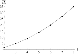
Figure 2: Energy per excess area of the deformed stated for low values of $l$

The ground states are represented by ellipsoidal (or quadrupole) deformations with $l=2$. Modulo its orientation with respect to the sphere, the ground state is three fold degenerate. One would expect this degeneracy to be lifted at higher orders in the perturbation.

Each of these perturbative states of the confined sphere will possess analogues in the full non-linear description. In particular, an infinite number of axially symmetric states solutions, one for each $l$, would be expected; ellipsoids, pears, and dumbbells (or discocytes) corresponding to $l=2,3,4$ respectively. A detailed analysis is beyond the scope of this paper but will be taken up elsewhere [20]. It would be interesting to know if cross talk between different values of $l$ emerges as non-perturbative features of the confinement process giving rise to composite structures such as (cup-shaped) stomatocytes.

The analysis of the confined elastic loop suggests that the simple dependence of the energy and the transmitted forces on the excess area will diverge from the simple behavior described here as the confined surface explores more of the hyperspherical volume and deviations from geodesic behavior become increasing pronounced.

In analogy with an elastic loop, it is reasonable to expect that the only stable weakly confined states are the ellipsoidal ground states with $l=2$. All excited states (with $l\geq 3$) are unstable. To show this, note that the second variation of the energy about a weakly confined state is given by

$$H_{2}\approx\frac{1}{2}\,\int d\Omega_{2}\,\Phi{\cal L}_{l}\Phi\,,$$ (40)

where the operator ${\cal L}_{l}$ is defined by

$${\cal L}_{l}=[\nabla_{0}^{2}+l(l+1)][\nabla_{0}^{2}+2]\,.$$ (41)

The eigenvalues of ${\cal L}_{l}$ are identified as

$$\lambda_{k}=(k(k+1)-l(l+1))(k(k+1)-2)\,.$$ (42)

These eigenvalues are plotted for $l=2,3,4$ and $5$ in Fig. 3.

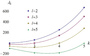
Figure 3: Eigenvalues of ${\cal L}$ for low values of $l$. Each point corresponds to $2k+1$ deformation modes on account of the spherical harmonics degeneracy

One observes that for each $l\geq 2$ there will be $l^{2}-4$ negative eigenvalues corresponding to unstable modes of decay. Thus, as claimed previously, the only stable states are those with $l=2$. This generalizes the qualitatively very similar stability analysis of loops weakly confined within a sphere [6]. Whether this behavior is a faithful representation of the behavior when the surface is not weakly confined, on the other hand, is anyone’s guess. Indeed, it will no longer be legitimate to assume that the ground state is completely attached.

4 Conclusions

In this paper, the confinement of a freely deformable closed two-dimensional surface within a three-dimensional hypersphere of smaller radius was examined. This is the natural generalization of a problem of a more domestic nature: the confinement of a loop within a surface. In the absence of the constraint the unique non-singular–topologically spherical–equilibrium state is a round sphere. Under confinement, this sphere deforms into one of an infinite number of equilibrium shapes; they have been examined in the limit of weak confinement. Mathematically, this problem can be viewed as a natural generalization of the spherical Willmore problem, to which it reduces when the constraint on the area is relaxed. In this context, it is also reasonable to expect that counterparts of these states exist in each topological sector of the two-dimensional surface.

While the study of confinement in higher dimensions is not expected–or is unlikely–to offer insight into problems that arise in biology or soft matter, the questions posed are of a fundamental nature that have not been explored previously. Indeed, if the geometrical invariants of a surface are ordered by derivatives, after area, the bending energy is arguably the most important–non-topological–invariant among them. Analogues of the problem could be relevant in relativistic field theories, be it the Euclidean formulation of such theories, or the behavior of stationary spacelike surface states. Analogous actions were discussed by Polyakov as effective field theories [10].

If the analysis of confined loops is any guide, a non-perturbative extension of this work should be worth pursuing. To this end, it is possible to exploit the conformal invariance of the two-dimensional bending energy [7] to reformulate the problem in a rather striking way. For under inversion in a hypersphere, itself located on the confining hypersphere, the latter will get mapped to a three-dimensional Euclidean hyperplane. The confined surface on the three-sphere is replaced by a surface that is free to bend in this three-dimensional space without obstruction. The area, however, is not invariant under conformal transformations; it gets replaced by a surface integral

$$A\to\int\,\frac{dA_{2}}{(|{\bf X}|^{2}+\frac{1}{4})^{2}}\,\,,$$ (43)

involving a potential that will depend on the Euclidean distance $|{\bf X}|$ from points on the surface to the origin of the three dimensional space. The confining surface is replaced by this potential.

It is also possible to consider confinement as a dynamical process in a relativistic theory of extended objects. Two-dimensional surfaces are interpreted now as the world-sheets of strings [21, 22]; the confining hypersphere is replaced by a three-dimensional de Sitter space, the fixed worldsheet of a membrane.

Appendix Appendix A Embedding identities

In this appendix, several useful identities connecting $\Gamma_{N},\Gamma_{N,N+1}$ and $\Sigma_{N+1}$, as defined in section 2, are collected.

Let ${\bf E}_{A},$ $A=1,\dots N+1$ be the tangent vectors to the hypersurface $\Sigma_{N+1}$, and ${\bf n}$ its normal vector. The Gauss structure equations describing the embedding of $\Sigma_{N+1}$ in Euclidean space are given by

$$\nabla_{A}{\bf E}_{B}=-K_{AB}{\bf n}\,.$$ (A.1)

Here $\nabla_{A}$ is the covariant derivative on $\Sigma_{N+1}$ compatible with its induced metric, $G_{AB}={\bf E}_{A}\cdot{\bf E}_{B}$. These equations define the curvature tensor $K_{AB}$.

The counterpart of Eq.(A.1), describing the embedding of the surface $\Gamma_{N}$ directly into the same Euclidean space, is given by

$$\nabla_{a}{\bf e}_{b}=-K_{ab\,I}\,{\bf n}^{I}\,.$$ (A.2)

Choose ${\bf n}_{1}={\bf n}$, and ${\bf n}_{2}={\bf l}$. The surface tangent vectors ${\bf e}_{a}$, $a=1,\cdots,N$ can be cast as a linear combination of their hypersurface counterparts as follows, ${\bf e}_{a}={\cal E}^{A}_{a}\,{\bf E}_{A}$, where ${\cal E}^{A}_{a}=\partial U^{A}/\partial s^{a}$. The vector ${\bf l}$ can likewise be expanded, ${\bf l}=l^{A}{\bf E}_{A}$.

Projecting $\nabla_{A}{\bf E}_{B}$ onto $\Gamma_{N}$ gives

$${\cal E}^{A}_{a}{\cal E}^{B}_{b}\nabla_{A}{\bf E}_{B}=\nabla_{a}{\bf e}_{b}-(\nabla_{a}{\cal E}_{b}^{B})\,{\bf E}_{B}\,.$$ (A.3)

It follows from the structure equation (A.1) and its definition, that the extrinsic curvature of $\Gamma_{N}$ associated with the rotations of ${\bf n}$ onto $\Gamma_{N}$ is given by Eq.(17), $K_{ab\,(1)}={\cal E}^{A}_{a}{\cal E}^{B}_{b}K_{AB}$. In particular, using the completeness of the basis vectors $\{{\cal E}^{A}_{a},l^{A}\}$, $g^{ab}{\cal E}^{A}_{a}{\cal E}^{B}_{b}+l^{A}l^{B}=G^{AB}$, the surface trace of $K_{(1)\,ab}$ is given by

$$K_{(1)}=g^{ab}{\cal E}^{A}_{a}{\cal E}^{B}_{b}K_{AB}=(G^{AB}-l^{A}l^{B})K_{AB}=K-l^{A}l^{B}K_{AB}\,.$$ (A.4)

In addition,

$${\cal E}^{A}_{a}l^{B}\nabla_{A}{\bf E}_{B}=\nabla_{a}{\bf l}-(\nabla_{a}l^{B}){\bf E}_{B}\,,$$ (A.5)

so that

$$\omega_{a\,12}:={\bf n}\cdot\nabla_{a}{\bf l}=-{\cal E}^{A}_{a}l^{B}K_{AB}\,.$$ (A.6)

If the surface is embedded in a hypersphere with $K_{AB}=G_{AB}$, then $K_{(1)\,ab}=g_{ab}$ and $\omega_{a\,12}=0$.

For a curve, with $N=1$, with unit tangent vector ${\bf T}=t^{A}{\bf E}_{A}$, $K_{(1)}=t^{A}t^{B}K_{AB}=\kappa_{n}$; $\omega_{12}=l^{A}t^{B}K_{AB}=\tau_{g}$, where $\kappa_{n}$ and $\tau_{g}$ are the normal curvature and geodesic torsion of the curve.

The counterpart of Eqs.(A.1) and (A.2) for $\Gamma_{N,N+1}$ embedded into $\Sigma_{N+1}$ are

$$D_{a}{\cal E}_{b}^{A}=-\kappa_{ab}\,l^{A}\,,$$ (A.7)

where

$$D_{a}{\cal E}_{b}^{C}:=\nabla_{a}{\cal E}^{C}_{b}+\Gamma^{C}_{\phantom{C}AB}{\cal E}^{A}_{a}{\cal E}^{B}_{b}\,,$$ (A.8)

and $\Gamma_{AB}^{C}$ is the Christoffel connection compatible with the induced metric on $\Sigma_{N+1}$, $G_{AB}$. Eq.(A.7) defines the extrinsic curvature tensor $\kappa_{ab}$ associated with the rotation of the normal ${\bf l}$ onto $\Gamma_{N}$. This provides the identity for $K^{(2)}_{ab}$,

$$K^{(2)}_{ab}:=\kappa_{ab}=-l_{B}D_{a}{\cal E}^{B}_{b}\,.$$ (A.9)

Appendix Appendix B Derivation of the stress tensor

In this appendix, the stress tensor introduced in Eq.(3) will be derived. This will be done by extending the auxiliary variables method introduced in [17] to co-dimensions higher than one. One constructs a functional $H_{c}[{\bf X},{\bf e}_{a},{\bf n},g_{ab},K_{ab},\omega_{a}^{\phantom{a}IJ},{\bf f}^{a},\lambda^{a}_{\phantom{a}I},\lambda_{IJ},\lambda^{ab},\Lambda^{ab}_{\phantom{ab}I},\Lambda^{a}_{\phantom{a}IJ}]$ treating the embedding functions ${\bf Y}$, the adapted basis $\{{\bf e}_{a},{\bf n}^{I}\}$, the metric tensor $g_{ab}$, the extrinsic curvature tensor $K^{I}_{ab}$, as well as the connection $\omega_{a}^{\phantom{a}IJ}$ as independent variables, by introducing Lagrange multipliers ${\bf f}^{a},\lambda^{a}_{\phantom{a}I},\lambda_{IJ},\lambda^{ab},\Lambda^{ab}_{\phantom{ab}I},\Lambda^{a}_{\phantom{a}IJ}$

$$H_{c} =\frac{1}{2}\int dA_{N}\,K_{I}\,K^{I}+\int dA_{N}\left[{\bf f}^{a}\cdot({\bf e}_{a}-\partial_{a}\,{\bf Y})+\lambda^{ab}(g_{ab}-{\bf e}_{a}\cdot{\bf e}_{b})+\frac{1}{2}\lambda_{IJ}(\delta^{IJ}-{\bf n}^{I}\cdot{\bf n}^{J})\right]$$

$$+\int dA_{N}\left[\lambda^{a}_{\phantom{a}I}{\bf e}_{a}\cdot{\bf n}^{I}+\Lambda^{ab}_{\phantom{ab}I}(K_{ab}^{\phantom{ab}I}-\partial_{a}{\bf n}^{I}\cdot{\bf e}_{b})+\Lambda^{a}_{\phantom{a}IJ}(\omega_{a}^{\phantom{a}IJ}-{\bf n}^{I}\cdot\partial_{a}{\bf n}^{J})\right]\,.$$ (B. 1)

The bending energy now depends only on the independent variables $g_{ab}$ and $K^{I}_{ab}$. Lagrange multipliers with more than one index possess the same symmetry as the quantities they multiply. Thus, for instance, $\lambda^{ab}=\lambda^{ba}$, $\lambda_{IJ}=\lambda_{JI}$, $\Lambda^{a}_{\phantom{a}IJ}=-\Lambda^{a}_{\phantom{a}JI}$. The variation of $H$ with respect to ${\bf Y}$ gives

$$\delta_{\bf X}H_{C}=\int dA_{N}\,\nabla_{a}{\bf f}^{a}\cdot\delta{\bf Y}\,.$$ (B. 2)

Thus, in equilibrium, ${\bf f}^{a}$ will be conserved on a free surface; it is identified as the stress tensor on the surface [17]. The Euler-Lagrange equations for ${\bf e}_{a}$ provide an expansion of the Lagrange multiplier ${\bf f}^{a}$ with respect to the adapted basis

$${\bf f}^{a}=\left(2\lambda^{ab}+\Lambda^{acI}K_{c\phantom{c}I}^{\phantom{c}b}\right){\bf e}_{b}-\left(\lambda^{aI}-\Lambda^{abJ}\omega_{bJ}^{\phantom{bJ}I}\right){\bf n}_{I}\,.$$ (B. 3)

The Euler-Lagrange equation for ${\bf n}$ is

$$(\lambda^{aI}+\nabla_{b}\Lambda^{abI}-2\Lambda^{bIJ}K_{b\phantom{a}J}^{\phantom{b}a}){\bf e}_{a}-(\nabla_{a}\Lambda^{aIJ}+\Lambda^{abI}K_{ab}^{\phantom{ab}J}+\lambda^{IJ}){\bf n}_{J}=0\,.$$ (B. 4)

Thus from the linear independence of the adapted basis, one identifies

$$\lambda^{aI}=-\nabla_{b}\Lambda^{abI}+2\Lambda^{bIJ}K_{b\phantom{a}J}^{\phantom{b}a}\,,\quad\lambda^{IJ}=-\nabla_{a}\Lambda^{aIJ}-\Lambda^{abI}K_{ab}^{\phantom{ab}J}\,.$$ (B. 5)

There remains to determine the three Lagrange multipliers $\lambda^{ab}$, $\Lambda^{abI}$ and $\Lambda^{aIJ}$. They are determined from the Euler-Lagrange equations for $g_{ab}$, $K_{abI}$ and $\omega_{a}^{\phantom{a}IJ}$ respectively:

$$\lambda^{ab}=K_{I}(K^{abI}-\frac{1}{4}K^{I}g^{ab})\,;\quad\Lambda^{abI}=-K^{I}g^{ab}\,;\quad\Lambda^{aIJ}=0\,.$$ (B. 6)

$\Lambda^{aIJ}$ vanishes because the connection $\omega_{a}^{\phantom{a}IJ}$ does not appear explicitly in the bending energy. Had the definition of $\omega_{a}^{\phantom{a}IJ}$ been omitted, no error would have been incurred. However, one would not be so lucky if the energy had depended explicitly on $\omega_{a}^{\phantom{a}IJ}$.

Substituting the expressions for the Lagrange multipliers given by Eqs. (B. 5) and (B. 6) into Eq.(B. 3), ${\bf f}^{a}$ assumes the form

$${\bf f}^{a}=K_{I}\left(K^{abI}-\frac{1}{2}K^{I}g^{ab}\right){\bf e}_{b}-\tilde{\nabla}^{a}K^{I}{\bf n}_{I}\,,$$ (B. 7)

where $\tilde{\nabla}_{a}$ is the covariant derivative involving the normal connection $\omega_{a\phantom{I}J}^{\phantom{a}I}$.

Appendix Appendix C Hypersurface adapted Euler-Lagrange derivatives

In this appendix, the details of the derivation of Eqs.(16a) and (16b) are provided. First dismantle the covariant Laplacian $\tilde{\nabla}^{2}K^{I}$ in terms of the normal connection, so that

$$\tilde{\nabla}^{2}K_{I} = g^{ab}\left(\nabla_{a}(\tilde{\nabla}_{b}K_{I})-\omega_{aIJ}\tilde{\nabla}_{b}K_{J}\right)$$ (C. 1)

$$= \nabla^{2}K_{I}+\nabla^{a}\omega_{aIJ}K^{J}+2\omega_{aIJ}\nabla^{a}K^{J}+\omega_{aI}^{\phantom{aI}J}\omega_{aJL}K^{L}\,.$$

The components along ${\bf n}$ and ${\bf l}$ are given respectively by

$$\tilde{\nabla}^{2}K^{(1)} = \nabla^{2}K_{(1)}+\kappa\nabla\cdot\omega+2\omega\cdot\nabla\kappa-|\omega|^{2}K_{(1)}\,;$$ (C. 2a)

$$\tilde{\nabla}^{2}\kappa = \nabla^{2}\kappa-K_{(1)}\nabla\cdot\omega-2\omega\cdot\nabla K_{(1)}-|\omega|^{2}\kappa\,.$$ (C. 2b)

where $\nabla\cdot\omega=\nabla^{a}\omega_{a12}$ is the divergence of the normal connection and $|\omega|^{2}=\omega^{a}_{\phantom{a}12}\omega_{a}^{\phantom{a}12}$ is its squared modulus. For an embedding in a hypersphere, the normal connection vanishes, $\omega_{a12}=0$, so that the normal covariant derivatives are replaced by covariant derivatives, $\tilde{\nabla}^{2}\kappa=\nabla^{2}\kappa$; in addition, $K_{(1)}$ is constant, so that $\tilde{\nabla}^{2}K_{(1)}=0$.

More generally, Eq. (A.6) is used to express the divergence and squared modulus of the normal connection in terms of hypersurface curvatures. The second term is given by

$$\nabla\cdot\omega: = \nabla^{a}\omega_{a12}=-\nabla^{a}({\cal E}_{a}^{A}l^{B}K_{AB})$$ (C. 3)

$$= \kappa l^{A}l^{B}K_{AB}-\kappa^{ab}{\cal E}_{a}^{A}{\cal E}_{b}^{B}K_{AB}-g^{ac}{\cal E}_{a}^{A}{\cal E}_{c}^{C}l^{B}\nabla_{C}K_{AB}$$

$$= \kappa l^{A}l^{B}K_{AB}-\kappa^{ab}K_{ab\,(1)}-{\cal H}^{AB}l^{C}\nabla_{C}K_{AB}\,.$$

Here ${\cal H}^{AB}=g^{ab}{\cal E}_{a}^{A}{\cal E}_{b}^{B}$ represents the projector onto $\Gamma_{N,N+1}$. On the second line, the relations $\nabla^{a}l^{B}=\kappa^{ab}{\cal E}_{b}^{B}$ and $D^{a}{\cal E}_{a}^{A}=-\kappa l^{A}$ are used, which follow from the structure equations associated with the embedding of the surface $\Gamma_{N,N+1}$ in $\Sigma_{N+1}$, (Eq. (A.9) and its contraction). In addition, the Codazzi-Mainardi equation for $\Sigma_{N+1}$, $\nabla_{A}K_{BC}=\nabla_{B}K_{AC}$ has been used in the third line.

The squared modulus is given by

$$|\omega|^{2}: = g^{ab}\omega_{a12}\omega_{b12}=g^{ab}{\cal E}_{a}^{A}{\cal E}_{b}^{B}l^{C}l^{D}K_{AC}K_{BD}$$ (C. 4)

$$= l^{A}l^{B}\left(K_{AC}K_{B}^{\phantom{B}C}-K_{AC}K_{BD}l^{C}l^{D}\right)$$

$$= l^{A}l^{B}\left(K_{(1)}K_{AB}-R_{AB}\right)\,,$$

where the completeness of the basis $\{{\cal E}^{A}_{a},l^{A}\}$ and the contracted Gauss-Codazzi equation have been used. Here $R_{AB}$ is the Ricci tensor constructed with the metric $G_{AB}$.

One also requires the decomposition of $K_{ab}^{\phantom{ab}I}f^{ab}$ where $f^{ab}={\bf f}^{a}\cdot{\bf e}^{b}=K_{I}(K^{abI}-1/2g^{ab}K^{I})$, which are given by

$$K_{ab}^{\phantom{ab}(1)}f^{ab} = K^{(1)}\left(K_{ab\,(1)}K^{ab\,(1)}-\frac{1}{2}K_{(1)}^{2}-\mu\right)+\kappa\left(\kappa_{ab}K^{ab\,(1)}-\frac{1}{2}\kappa K^{(1)}\right)\,;$$ (C. 5a)

$$\kappa_{ab}f^{ab} = K^{(1)}\left(\kappa_{ab}K^{ab\,(1)}-\frac{1}{2}\kappa K^{(1)}\right)+\kappa\left(\kappa_{ab}\kappa^{ab}-\frac{1}{2}\kappa^{2}-\mu\right)\,.$$ (C. 5b)

For a surface embedded in a hypersphere, with $K_{ab}^{\phantom{ab}(1)}=g_{ab}$, $\kappa\left(\kappa_{ab}K^{(1)\,ab}-\kappa K^{(1)}/2\right)=-(N-2)\kappa^{2}/2$ and $K^{(1)}\left(K_{ab\,(1)}K^{ab\,(1)}-K_{(1)}^{2}/2\right)=-N^{2}(N-2)/2$.

For confined curves, with $K^{(1)}=\kappa_{n}$ and $\kappa=\kappa_{g}$, Eq, (C. 5a) reduces to $\kappa_{n}[(\kappa_{g}^{2}+\kappa_{n}^{2})/2-\mu]$, whereas Eq.(C. 5b) reduces to $\kappa_{g}[(\kappa_{g}^{2}+\kappa_{n}^{2})/2-\mu]$.

Appendix Appendix D Variational principle adapted to a hypersphere

It is instructive to decompose the bending energy into parts adapted to its confined environment. Using Eqs.(A.4) and (A.9) one finds

$$H=\frac{1}{2}\,\int dA_{N}\,K^{(I)}K_{(I)}=\frac{1}{2}\,\int dA_{N}\,[\kappa^{2}+(K-l^{A}l^{B}K_{AB})^{2}]\,.$$ (D. 1)

The first term is the bending energy of the surface embedded into the three-dimensional curved geometry described by the metric tensor $G_{AB}$,

$$H_{0}=\frac{1}{2}\,\int dA_{N}\,\kappa^{2}\,.$$ (D. 2)

The second is the bending energy inherited from the hypersurface. This is the generalization to higher dimensions of the Pythagorean decomposition of the Frenet curvature $k$ of a space curve into geodesic and normal parts, $k^{2}=\kappa_{g}^{2}+\kappa_{n}^{2}$ familiar in the theory of surfaces [5].

The Euler Lagrange equation for the surface $s\to U(s)$ described by the bending energy (D. 2) is given by

$$-\,\nabla^{2}\kappa+\frac{1}{2}(\kappa^{2}-2\kappa_{ab}\kappa^{ab})\kappa-R_{AB}l^{A}l^{B}\kappa+\mu\kappa=0\,.$$ (D. 3)

This equation was derived in the 90s in the context of relativistic extended objects [19].

For an $N+1$-sphere, the Ricci tensor is proportional to the metric tensor, $R_{AB}=NG_{AB}$ so that $R_{AB}l^{A}l^{B}=N$. In this case $K_{AB}=G_{AB}$, and $K=N+1$ so that Eq. (D. 1) then reduces to

$$H=\frac{1}{2}\,\int dA_{N}\,[\kappa^{2}+N^{2}]\,.$$ (D. 4)

The contribution to the energy density due to the normal curvature is constant. If the Euler-Lagrange derivative corresponding to this contribution ($N^{2}\kappa/2$) is added on the left hand side of Eq. (D. 3), the shape equation Eq. (23) is reproduced.

Appendix Appendix E Rotational invariance and confinement by a hypersphere

If the confining surface is a hypersphere, the Euler Lagrange equations will respect rotational invariance in $\mathbb{R}^{4}$. Thus, whereas stress is not conserved, torques will be, corresponding as they do to the Noether current associated with the rotational symmetry of the energy.

Consider a small rotation about the origin $\delta X^{i}=\epsilon^{ijkl}\Omega^{jk}X^{l}$, characterized by the antisymmetric rotation matrix $\Omega^{ij}$, where $\epsilon^{ijkl}$ is the Levi-Civita symbol and $i,j,k,l=1,\dots,4$ index tensors in Euclidean space $\mathbb{R}^{4}$. Each of the two normal vectors ${\bf n}^{I},I=1,2$ rotates accordingly: $\delta{n}^{Ii}=\epsilon^{ijkl}\Omega^{jk}n^{Il}$. It can be shown that, in equilibrium, on any surface patch

$$\delta H_{c}=-\Omega^{ij}\,\int dA_{2}\,\nabla_{a}m^{ij\,a}\,,$$ (E. 1)

where

$$m^{aij}=\epsilon^{ijkl}\left(f^{ak}X^{l}-K_{I}g^{ab}e^{k}_{b}n^{Il}\right)\,.$$ (E. 2)

Here $f^{ak}={\bf f}^{a}\cdot\hat{\bf x}^{k}$, $e_{a}^{k}={\bf e}_{a}\cdot\hat{\bf x}^{k}$, etc.

Thus $m^{ij\,a}$ is conserved if $H_{c}$ is rotationally invariant. This is confirmed by the following calculation:

$$\nabla_{a}m^{aij}=\epsilon^{ijkl}\left(\nabla_{a}f^{ak}X^{l}+f^{ak}e^{l}_{a}-K_{I}K^{Iab}e^{k}_{a}e^{l}_{b}-\tilde{\nabla}_{a}K_{I}g^{ab}e^{k}_{b}n^{Il}-K_{I}K_{J}n^{Jk}n^{Il}\right)\,.$$ (E. 3)

In general, all but the first term either vanish identically or cancel among themselves. For the first term one has $\epsilon^{ijkl}\nabla_{a}f^{ak}X^{l}=\epsilon^{ijkl}\varepsilon_{\bf n}n^{k}X^{l}$. However, if the surface is confined to a unit hypersphere centered on the origin, so that ${\bf X}={\bf n}$, this term also vanishes.

It is not obvious how to exploit this invariance in a manner analogous to that in the treatment of a polymer confined within a sphere. In any case a better strategy is to exploit the conformal invariance of the two-dimensional bending energy, as sketched in section 4.

References

- [1] Manning G S 1987 Quart. Appl. Math. 45 515
- [2] Nickerson H K and Manning G S 1988 Geometria Dedicata 27 127
- [3] Spakowitz A J and Z G Wang 2003 Phys. Rev. Lett. 91, 166102
- [4] Kamien R 2002 Rev. Mod. Phys. 74, 953
- [5] Do Carmo M 1976 Differential Geometry of Curves and Surfaces (Prentice hall)
- [6] Guven J and Vázquez-Montejo P 2012 Phys. Rev. E 85, 026603
- [7] Willmore T J 1982 Total Curvature in Riemannian Geometry (Chichester: Ellis Horwood)
- [8] Palmer B 2008 Variational Problems which are Quadratic in the Surface Curvatures AIP Conf. Proc. 1002, 33, DOI:10.1063/1.2918094
- [9] Landau L D and Lifshitz E M 1999 Theory of Elasticity (Butterworth-Heinemann, Oxford).
- [10] Polyakov A M 1987 Gauge Fields and Strings (Chur, Switzerland: Harwood Academic Publishers)
- [11] Canham P 1970 J. Theor. Biol. 26 61; Helfrich W 1973 Z. Naturforsch. C 28 693
- [12] Seifert U 1991 J. Phys. A:Math and Gen.24 L573; Jülicher F, Seifert U and Lipowsky R 1993 Phys. Rev. Lett. 71 452
- [13] Kahraman O, Stoop N and Muller M M 2012 Europhys Lett. 97 68008
- [14] Kahraman O, Stoop N and Muller M M 2012 To be published in New J. Phys.
- [15] Spivak M 1979 A Comprehensive Introduction to Differential Geometry. Vol. 5, Second Edition (Houston: Publish or Perish Inc.)
- [16] Capovilla R and Guven J 2002 J. Phys. A: Math. Gen. 35 6233
- [17] Guven J 2004 J. Phys. A: Math and Gen. 37 L313
- [18] Langer J and Singer D A 1984 J. Diff. Geom. 20, 1
- [19] Capovilla R and Guven J 1995 Phys. Rev. D 51, 6736
- [20] Guven J and and Vázquez-Montejo P 2012 In preparation
- [21] Vilenkin A and Shellard E P S 1994 Cosmic Strings and Other Topological Defects (Cambridge Monographs on Mathematical Physics)
- [22] Green M B, Schwarz J H and Witten E 1987 Superstring Theory, Vol. 1 (Cambridge University Press)