State-independent experimental tests of quantum contextuality in a three dimensional system

Xiang Zhang1, Mark Um1, Junhua Zhang1, Shuoming An1, Ye Wang1, Dong-ling Deng1,2, Chao Shen1,2, Luming Duan1,2, Kihwan Kim1 kimkihwan@gmail.com 1 Center for Quantum Information, Institute for Interdisciplinary Information Sciences, Tsinghua University, Beijing 100084, P. R. China 2 Michigan Center for Theoretical Physics and Department of Physics, University of Michigan, Ann Arbor, MI 48109, USA
(March 8, 2024)
Abstract

We experimentally observed state-independent violations of Kochen-Specker inequalities for the simplest indivisible quantum system manifesting quantum contextuality, a three-level (qutrit) system. We performed the experiment with a single trapped Yb+171superscriptsuperscriptYb171{}^{171}\mathrm{Yb}^{+}\leavevmode\nobreak\ ion, by mapping three ground states of the Yb+171superscriptsuperscriptYb171{}^{171}\mathrm{Yb}^{+}\leavevmode\nobreak\ ion to a qutrit system and carrying out quantum operatations by applying microwaves resonant to the qutrit transition frequencies. Our results are free from the detection loophole and cannot be explained by the non-contextual hidden variable models.

pacs:
03.65.-w, 03.65.Ud, 37.10.Ty, 32.50.+d

It is a long-standing problem whether the nature of physical system would be completely described by quantum mechanics. In classical views the measurement outcomes on physical properties are non-contextual, i.e.formulae-sequence𝑖𝑒\it{i.e.}, predetermined independently of their own and other simultaneous compatible measurements, while quantum mechanics is contextual. Kochen, Specker and Bell proved that quantum mechanics and any non-contextual classical theory are in conflict Kochen and Specker (1967); Bell (1966), deeply rooted in the essence of quantum mechanics regardless of states of the system. The original logical proof has been formulated to experimentally testable inequalities, called Kochen-Specker (KS) inequalities. The Bell’s inequalities that hold for classical theories with local hidden variables can be considered as a special type of KS inequalities, where the contextuality is presented by non-locality. While Bell’s inequalities can be violated by special entangled states in space-like separation, the violation of KS inequalities could be observed by any quantum state in a system with dimension d3𝑑3d\geq 3. For cases where d4𝑑4d\geq 4, KS inequalities were proposed Mermin (1990); Peres (1991); Cabello (2008) and demonstrated in both a state-dependent Michler et al. (2000); Huang et al. (2003); Bartosik et al. (2009) and a state-independent manner Kirchmair et al. (2009); Amselem et al. (2009); Moussa et al. (2010). For the smallest case d=3𝑑3d=3, the state-dependent inequality was developed Klyachko et al. (2008) and tested with a photon system Lapkiewicz et al. (2011). Lately, the state-independent inequality was found Yu and Oh (2012); Cabello et al. (2012) and the violations were informed with also a photon system Zu et al. (2012). However, these experimental demonstrations are open to the detection loophole. Here we report the experimental results of a single three-level atomic ion that are in conflict with non-contextual classical theories. The experimental violations of KS inequalities are observed independently of entanglement or superposition of the states and confirm the quantum contextuality at the most simple and fundamental level without the fair sampling assumption.

In noncontextual classical models, values of an observable are determined by only a hidden variable independently of the measurement context, i.e.formulae-sequence𝑖𝑒\it{i.e.}, set of mutually compatible observables measured in a single experimental setting. The observables are compatible if their results are not dependent on the order of measurements. Kochen and Specker showed that any quantum state in larger than 2 dimensions would reveal conflict with the non-contextual theories. The demonstration of the conflict in a simplest three dimensional quantum system, a qutrit, has fundemental importance since it would naturally imply the contraction in higher dimensions. However, the original proof of KS theorem for a qutrit involves too many configurations, 117 observables, to be verified in experiment Kochen and Specker (1967). Differently from the KS proof, Yu and Oh realized a KS inequality of a qutrit with 13 observables and 24 correlations of them Yu and Oh (2012). It has been proved that 13 settings are minimum for KS tests of d=3𝑑3d=3 system Cabello (2011) and the bound have improved to be tight, which is favorable in experimental realization Cabello et al. (2012).
Refer to caption
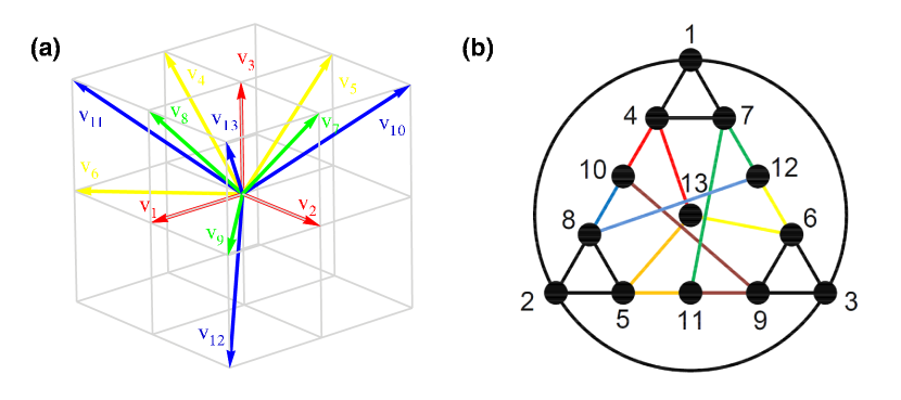
Figure 1: Observables and compatiblity relations for the state-independent inequality of a qutrit. (a) The 13 observables are represented as vectors in a 3-dimensional space. |viketsubscript𝑣𝑖\left|v_{i}\right\rangles are specified as v1=(1,0,0)subscript𝑣1100v_{1}=\left(1,0,0\right), v2=(0,1,0)subscript𝑣2010v_{2}=(0,1,0), v3=(0,0,1)subscript𝑣3001v_{3}=(0,0,1), v4=(0,1,1)subscript𝑣4011v_{4}=(0,1,-1), v5=(1,0,1)subscript𝑣5101v_{5}=(1,0,-1), v6=(1,1,0)subscript𝑣6110v_{6}=(1,-1,0), v7=(0,1,1)subscript𝑣7011v_{7}=(0,1,1), v8=(1,0,1)subscript𝑣8101v_{8}=(1,0,1), v9=(1,1,0)subscript𝑣9110v_{9}=(1,1,0), v10=(1,1,1)subscript𝑣10111v_{10}=(-1,1,1), v11=(1,1,1)subscript𝑣11111v_{11}=(1,-1,1), v12=(1,1,1)subscript𝑣12111v_{12}=(1,1,-1), and v13=(1,1,1)subscript𝑣13111v_{13}=(1,1,1). (b) The compatibility graph between 13 observables. The nodes represent the 13 vectors visubscript𝑣𝑖v_{i} and the edges show the orthogonality or compatibility relations. The experimental realization and joint measurements of the orthogonal observables are described in Table 1.

The inequalities with 13 observables are represented in the Hilbert space of a qutrit with basis {|1,|2,|3}ket1ket2ket3\left\{\left|1\right\rangle,\left|2\right\rangle,\left|3\right\rangle\right\}. The form of the observable is Ai=I2Visubscript𝐴𝑖𝐼2subscript𝑉𝑖A_{i}=I-2V_{i}, where Visubscript𝑉𝑖V_{i} is the normalized projection operator on a vector |vi=a|1+b|2+c|3ketsubscript𝑣𝑖𝑎ket1𝑏ket2𝑐ket3\left|v_{i}\right\rangle=a\left|1\right\rangle+b\left|2\right\rangle+c\left|3\right\rangle. The 13 vectors required for the inequality are displayed in 3d𝑑d Hilbert space in Fig. 1(a), where the values (a,b,c)𝑎𝑏𝑐(a,b,c) of a vector, |viketsubscript𝑣𝑖\left|v_{i}\right\rangle are assigned as real numbers, which are enough to cover all possible projections in a qutrit space. In Fig. 1(b) a edge (i,j)E𝑖𝑗𝐸\left(i,j\right)\in E shows the orthogonal relation of nodes i,jV𝑖𝑗𝑉i,j\in V, where Aisubscript𝐴𝑖A_{i} and Ajsubscript𝐴𝑗A_{j} are compatible observables. There are 24 edges requiring simultaneous measurements. The tight ineqaulity is written as Cabello et al. (2012),

χ13delimited-⟨⟩subscript𝜒13\displaystyle\left\langle\chi_{13}\right\rangle =\displaystyle= iVμiAi(i,j)EμijAiAjsubscript𝑖𝑉subscript𝜇𝑖delimited-⟨⟩subscript𝐴𝑖subscript𝑖𝑗𝐸subscript𝜇𝑖𝑗delimited-⟨⟩subscript𝐴𝑖subscript𝐴𝑗\displaystyle\sum_{i\in V}\mu_{i}\left\langle A_{i}\right\rangle-\sum_{\left(i,j\right)\in E}\mu_{ij}\left\langle A_{i}A_{j}\right\rangle (1)
\displaystyle- (i,j,k)CμijkAiAjAk25,subscript𝑖𝑗𝑘𝐶subscript𝜇𝑖𝑗𝑘delimited-⟨⟩subscript𝐴𝑖subscript𝐴𝑗subscript𝐴𝑘25\displaystyle\sum_{\left(i,j,k\right)\in C}\mu_{ijk}\left\langle A_{i}A_{j}A_{k}\right\rangle\leq 25,

where delimited-⟨⟩\left\langle\ldots\right\rangle denotes the average of measurement outcomes, μi=1(i=1,2,,9)subscript𝜇𝑖1𝑖129\mu_{i}=1\leavevmode\nobreak\ \left(i=1,2,\cdots,9\right), 2(i=10,,13)2𝑖10132\leavevmode\nobreak\ \left(i=10,\cdots,13\right), and μij=1subscript𝜇𝑖𝑗1\mu_{ij}=1, when (i,j)𝑖𝑗\left(i,j\right) are in the triangles {(1,4,7),(2,5,8),(3,6,9)}147258369\left\{(1,4,7),(2,5,8),(3,6,9)\right\}, 222 otherwise. Here C𝐶C is the set of four triangles in Fig. 1(a) and μijk=3subscript𝜇𝑖𝑗𝑘3\mu_{ijk}=3, when (i,j,k){(1,4,7),(2,5,8),(3,6,9)}𝑖𝑗𝑘147258369\left(i,j,k\right)\in\left\{(1,4,7),(2,5,8),(3,6,9)\right\} and 00 otherwise. The inequality is easily derived from an equation of the same form with 13 arbitrary variables that have ±1plus-or-minus1\pm 1. In quantum mechanics, χ13=(25+83)Isubscript𝜒132583𝐼\chi_{13}=\left(25+\frac{8}{3}\right)I, which clearly violates the inequality (1) with any input states in the 3d𝑑d Hilbert space.

For the hidden variable models that preserve algebraic structures of compatible observables, the inequality would be simplified to Yu and Oh (2012),

χ4=i=1013Vi1.delimited-⟨⟩subscript𝜒4superscriptsubscript𝑖1013delimited-⟨⟩subscript𝑉𝑖1\left\langle\chi_{4}\right\rangle=\sum_{i=10}^{13}\left\langle V_{i}\right\rangle\leq 1. (2)

The inequality is valid, assuming the product rule and the sum rule still hold. The product rule means the product of compatible observables are zero and the sum rule means the sum of all compatible observables are one. The χ4=(1+13)Isubscript𝜒4113𝐼\chi_{4}=\left(1+\frac{1}{3}\right)I for the quantum mechanics, which breaks the inequality (2) regardless of initial states.

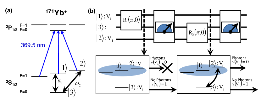
We performed the tests of the KS inequalities (1) and (2) with a single trapped Yb+171superscriptsuperscriptYb171{}^{171}\mathrm{Yb}^{+}\leavevmode\nobreak\ ion in a four-rods radio frequency trap similar to the one in Ref. [Olmschenk et al. (2007)]. A trapped ion system would be an exemplary candidate for the test of the quantum contextuality, since the system has already demonstrated near-perfect state initialization, state detection, and quantum operations on a qubit system Liebfried et al. (2003); Häffner et al. (2008); Acton (2008). A pair of qubits in a trapped ion system were already used to study the quantum contextuality of 4d𝑑d Hilbert space Kirchmair et al. (2009). We map the three internal levels of the Yb+171superscriptsuperscriptYb171{}^{171}\mathrm{Yb}^{+}\leavevmode\nobreak\ ion in the S1/2subscript𝑆12S_{1/2} ground state manifold to the qutrit states, which are represented by: |1=|F=1,mF=0ket1ketformulae-sequence𝐹1subscript𝑚𝐹0\left|1\right\rangle=\left|F=1,m_{F}=0\right\rangle, |2=|F=1,mF=1ket2ketformulae-sequence𝐹1subscript𝑚𝐹1\left|2\right\rangle=\left|F=1,m_{F}=1\right\rangle, and |3=|F=0,mF=0ket3ketformulae-sequence𝐹0subscript𝑚𝐹0\left|3\right\rangle=\left|F=0,m_{F}=0\right\rangle shown in Fig 2(a).

The initialization of the qutrit system can be realized by the same standard optical pumping as on a qubit. The operation on a single qutrit would be performed through the application of either resonant microwaves or lasers, depending on transitions. The quantum operations on internal levels of an atomic ion have been extremely well developed and demonstrated to a near-perfect level Brown et al. (2011). However, it is challenging to simultaneously discriminate between three states of a qutrit with decent detection fidelity in trapped ion systems. The standard detection method based on qubit-state-dependent fluorescence enables us to differentiate between one state versus the other two states of a qutrit. We observe on average 10 photons for the |1ket1\left|1\right\rangle or the |2ket2\left|2\right\rangle state and detect no photon for the |3ket3\left|3\right\rangle state. And by exchanging populations between |1ket1\left|1\right\rangle and |3ket3\left|3\right\rangle (or |2ket2\left|2\right\rangle and |3ket3\left|3\right\rangle), we could discriminate |2ket2\left|2\right\rangle and |3ket3\left|3\right\rangle versus |1ket1\left|1\right\rangle (or |1ket1\left|1\right\rangle and |3ket3\left|3\right\rangle versus |2ket2\left|2\right\rangle. However it is not possible to simultaneously distinguish the three states at our current experimental setting. In summary, we assign the value 1 on |3ket3\left|3\right\rangle state when no photons are detected and put the value 0 when photons are detected.
Refer to caption
Figure 2: The Yb+171superscriptsuperscriptYb171{}^{171}\mathrm{Yb}^{+}\leavevmode\nobreak\ ion system and the measurement scheme. (a) The energy diagram of Yb+171superscriptsuperscriptYb171{}^{171}\mathrm{Yb}^{+}\leavevmode\nobreak\ . Qutrit states |1ket1\left|1\right\rangle, |2ket2\left|2\right\rangle, and |3ket3\left|3\right\rangle are mapped onto |F=1,mF=0ketformulae-sequence𝐹1subscript𝑚𝐹0\left|F=1,m_{F}=0\right\rangle, |F=1,mF=1ketformulae-sequence𝐹1subscript𝑚𝐹1\left|F=1,m_{F}=1\right\rangle, and |F=0,mF=0ketformulae-sequence𝐹0subscript𝑚𝐹0\left|F=0,m_{F}=0\right\rangle in the S1/2subscript𝑆12S_{1/2} ground state manifold, respectively. The transition frequencies are: ω1=(2π)12642.8213subscript𝜔12𝜋12642.8213\omega_{1}=(2\pi)12642.8213 MHz and ω2=ω1+(2π)7.6372subscript𝜔2subscript𝜔12𝜋7.6372\omega_{2}=\omega_{1}+(2\pi)7.6372 MHz. The quantum operations are performed by the resonant microwaves. The detection laser beams are shown as blue lines. Here the quantum state projected to |1ket1\left|1\right\rangle or |2ket2\left|2\right\rangle generates fluoresence, while the state collapsed to |3ket3\left|3\right\rangle does not generate photons. Therefore, we assign zero on the observable related to state |3ket3\left|3\right\rangle when we detect photons and one when no photons are detected. (b) The sequential measurement scheme to construct the correlation terms ViVjdelimited-⟨⟩subscript𝑉𝑖subscript𝑉𝑗\left\langle V_{i}V_{j}\right\rangle. The three lines of the upper part stand for the three levels of Yb+171superscriptsuperscriptYb171{}^{171}\mathrm{Yb}^{+}\leavevmode\nobreak\ ion. First, we rotate the measurement axis to map the observables Visubscript𝑉𝑖V_{i} and Vjsubscript𝑉𝑗V_{j}, for example, on the state |1ket1\left|1\right\rangle and |2ket2\left|2\right\rangle, respectively. We transfer the Visubscript𝑉𝑖V_{i} on the state |3ket3\left|3\right\rangle and apply the standard flueorescent detection scheme. If we detect photons, the state should not be |3ket3\left|3\right\rangle and we assign zero on the observable Visubscript𝑉𝑖V_{i}. Therefore the correlation ViVjsubscript𝑉𝑖subscript𝑉𝑗V_{i}V_{j} should be zero and no further experiments are necessary. If we detect no photons, we assign one on the Visubscript𝑉𝑖V_{i}. To measure the value of Vjsubscript𝑉𝑗V_{j}, we apply the swapping microwave pulse that converts Vjsubscript𝑉𝑗V_{j} to |3ket3\left|3\right\rangle and the detection laser beam. If we observe photons, Vj=0subscript𝑉𝑗0V_{j}=0 and if no photons, Vj=1.subscript𝑉𝑗1V_{j}=1. By repeating the same experimental sequences and counting the number of experiments that detect no photons at the second measurement, we can obtain the average of the correlations ViVjsubscript𝑉𝑖subscript𝑉𝑗V_{i}V_{j}. We perform these sequencial detection schemes on the all the measurement settings listed in Table 1 for each initial state.
|1ket1\left|1\right\rangle |2ket2\left|2\right\rangle |3ket3\left|3\right\rangle Rotations Sequences (1stsuperscript1𝑠𝑡1^{st} 2ndsuperscript2𝑛𝑑2^{nd} 3rdsuperscript3𝑟𝑑3^{rd})
M1subscript𝑀1M_{1} V1subscript𝑉1V_{1} V2subscript𝑉2V_{2} V3subscript𝑉3V_{3} no rotation
M2subscript𝑀2M_{2} V5subscript𝑉5V_{5} V2subscript𝑉2V_{2} V8subscript𝑉8V_{8} R1(π/2,π)subscript𝑅1𝜋2𝜋R_{1}\left(\pi/2,\pi\right)
M3subscript𝑀3M_{3} V1subscript𝑉1V_{1} V4subscript𝑉4V_{4} V7subscript𝑉7V_{7} R2(π/2,0)subscript𝑅2𝜋20R_{2}\left(\pi/2,0\right)
M4subscript𝑀4M_{4} V9subscript𝑉9V_{9} V3subscript𝑉3V_{3} V6subscript𝑉6V_{6} R2(π,π)R1(π/2,π)subscript𝑅2𝜋𝜋subscript𝑅1𝜋2𝜋R_{2}\left(\pi,\pi\right)R_{1}\left(\pi/2,\pi\right)
M5subscript𝑀5M_{5} V4subscript𝑉4V_{4} V10subscript𝑉10V_{10} R2(π/2,0)R1(α,0)subscript𝑅2𝜋20subscript𝑅1𝛼0R_{2}\left(\pi/2,0\right)R_{1}\left(\alpha,0\right)
M6subscript𝑀6M_{6} V4subscript𝑉4V_{4} V13subscript𝑉13V_{13} R2(π/2,0)R1(α,π)subscript𝑅2𝜋20subscript𝑅1𝛼𝜋R_{2}\left(\pi/2,0\right)R_{1}\left(\alpha,\pi\right)
M7subscript𝑀7M_{7} V5subscript𝑉5V_{5} V11subscript𝑉11V_{11} R1(π/2,π)R2(α,π)subscript𝑅1𝜋2𝜋subscript𝑅2𝛼𝜋R_{1}\left(\pi/2,\pi\right)R_{2}\left(\alpha,\pi\right)
M8subscript𝑀8M_{8} V5subscript𝑉5V_{5} V13subscript𝑉13V_{13} R1(π/2,π)R2(α,0)subscript𝑅1𝜋2𝜋subscript𝑅2𝛼0R_{1}\left(\pi/2,\pi\right)R_{2}\left(\alpha,0\right)
M9subscript𝑀9M_{9} V6subscript𝑉6V_{6} V12subscript𝑉12V_{12} R2(π,0)R1(π/2,π)R2(α,0)subscript𝑅2𝜋0subscript𝑅1𝜋2𝜋subscript𝑅2𝛼0R_{2}\left(\pi,0\right)R_{1}\left(\pi/2,\pi\right)R_{2}\left(\alpha,0\right)
M10subscript𝑀10M_{10} V6subscript𝑉6V_{6} V13subscript𝑉13V_{13} R2(π,π)R1(π/2,0)R2(πα,0)subscript𝑅2𝜋𝜋subscript𝑅1𝜋20subscript𝑅2𝜋𝛼0R_{2}\left(\pi,\pi\right)R_{1}\left(\pi/2,0\right)R_{2}\left(\pi-\alpha,0\right)
M11subscript𝑀11M_{11} V7subscript𝑉7V_{7} V11subscript𝑉11V_{11} R2(π/2,π)R1(α,π)subscript𝑅2𝜋2𝜋subscript𝑅1𝛼𝜋R_{2}\left(\pi/2,\pi\right)R_{1}\left(\alpha,\pi\right)
M12subscript𝑀12M_{12} V12subscript𝑉12V_{12} V7subscript𝑉7V_{7} R2(π/2,π)R1(πα,π)subscript𝑅2𝜋2𝜋subscript𝑅1𝜋𝛼𝜋R_{2}\left(\pi/2,\pi\right)R_{1}\left(\pi-\alpha,\pi\right)
M13subscript𝑀13M_{13} V8subscript𝑉8V_{8} V10subscript𝑉10V_{10} R1(π/2,0)R2(α,0)subscript𝑅1𝜋20subscript𝑅2𝛼0R_{1}\left(\pi/2,0\right)R_{2}\left(\alpha,0\right)
M14subscript𝑀14M_{14} V8subscript𝑉8V_{8} V12subscript𝑉12V_{12} R1(π/2,0)R2(πα,0)subscript𝑅1𝜋20subscript𝑅2𝜋𝛼0R_{1}\left(\pi/2,0\right)R_{2}\left(\pi-\alpha,0\right)
M15subscript𝑀15M_{15} V10subscript𝑉10V_{10} V9subscript𝑉9V_{9} R1(π,0)R2(π/2,0)R1(πα,0)subscript𝑅1𝜋0subscript𝑅2𝜋20subscript𝑅1𝜋𝛼0R_{1}\left(\pi,0\right)R_{2}\left(\pi/2,0\right)R_{1}\left(\pi-\alpha,0\right)
M16subscript𝑀16M_{16} V9subscript𝑉9V_{9} V11subscript𝑉11V_{11} R1(π,π)R2(π/2,π)R1(α,0)subscript𝑅1𝜋𝜋subscript𝑅2𝜋2𝜋subscript𝑅1𝛼0R_{1}\left(\pi,\pi\right)R_{2}\left(\pi/2,\pi\right)R_{1}\left(\alpha,0\right)
R1(θ1,ϕ1)=(cosθ120eiϕ1sinθ12010eiϕ1sinθ120cosθ12)subscript𝑅1subscript𝜃1subscriptitalic-ϕ1subscript𝜃120superscript𝑒𝑖subscriptitalic-ϕ1subscript𝜃12010superscript𝑒𝑖subscriptitalic-ϕ1subscript𝜃120subscript𝜃12R_{1}\!\left(\theta_{1}\!,\phi_{1}\!\right)\!=\!\left(\begin{array}[]{ccc}\!\text{$\cos$}\frac{\theta_{1}}{2}\!&0&e^{i\phi_{1}}\text{$\sin$}\frac{\theta_{1}}{2}\\ \!0\!&1&0\\ \!-e^{-i\phi_{1}}\text{$\sin$}\frac{\theta_{1}}{2}\!&0&\text{$\cos$}\frac{\theta_{1}}{2}\end{array}\right)
R2(θ2,ϕ2)=(1000cosθ22eiϕ2sinθ220eiϕ2sinθ22cosθ22)subscript𝑅2subscript𝜃2subscriptitalic-ϕ21000subscript𝜃22superscript𝑒𝑖subscriptitalic-ϕ2subscript𝜃220superscript𝑒𝑖subscriptitalic-ϕ2subscript𝜃22subscript𝜃22R_{2}\!\left(\theta_{2}\!,\phi_{2}\!\right)\!=\!\left(\begin{array}[]{ccc}\!1&0&0\\ 0&\text{$\cos$}\frac{\theta_{2}}{2}&-e^{-i\phi_{2}}\text{$\sin$}\frac{\theta_{2}}{2}\\ 0&e^{i\phi_{2}}\text{$\sin$}\frac{\theta_{2}}{2}&\text{$\cos$}\frac{\theta_{2}}{2}\end{array}\right)
Table 1: Experimental measurement settings for the 24 joint probabilities of 13 observables. We rotate the 3-dimentional coordinates to map at least two orthogonal observables on the axes of the measurement basis {|1,|2,|3}ket1ket2ket3\left\{\left|1\right\rangle,\left|2\right\rangle,\left|3\right\rangle\right\}. Here Vi(i=1,2,,13)subscript𝑉𝑖𝑖1213V_{i}\leavevmode\nobreak\ (i=1,2,\cdots,13) stands for the projection observables on the vectors visubscript𝑣𝑖v_{i} shown in Fig. 1(a). These 16 settings contain all the joint measurements shown in Fig. 1(b) as edges. The rotations R1(θ1,ϕ1),R2(θ2,ϕ2)subscript𝑅1subscript𝜃1subscriptitalic-ϕ1subscript𝑅2subscript𝜃2subscriptitalic-ϕ2R_{1}\left(\theta_{1},\phi_{1}\right),R_{2}\left(\theta_{2},\phi_{2}\right) are realized by applying microwave pulses with the frequencies of ω1subscript𝜔1\omega_{1} and ω2subscript𝜔2\omega_{2}, which are resonant to the transitions between |1ket1\left|1\right\rangle and |3ket3\left|3\right\rangle and between |2ket2\left|2\right\rangle and |3ket3\left|3\right\rangle, respectively, where θ1subscript𝜃1\theta_{1}, θ2subscript𝜃2\theta_{2} and ϕ1subscriptitalic-ϕ1\phi_{1}, ϕ2subscriptitalic-ϕ2\phi_{2} are controlled by the duration and the phase of the applied microwaves. Here, α𝛼\alpha represents 0.392π.0.392𝜋0.392\pi. Note that each observable will be transferred to the state |3ket3\left|3\right\rangle just before the measurement, since we only assign the values on the state |3.ket3\left|3\right\rangle.

It is straightforward to measure the average values of single observables, Aidelimited-⟨⟩subscript𝐴𝑖\left\langle A_{i}\right\rangle in Eq. (1) and (2). We rotate the measurement axis visubscript𝑣𝑖v_{i} to the state |3ket3\left|3\right\rangle and then measure the probability of the state P|3subscript𝑃ket3P_{\left|3\right\rangle} (=Viabsentdelimited-⟨⟩subscript𝑉𝑖=\left\langle V_{i}\right\rangle), corresponding to the values of Aidelimited-⟨⟩subscript𝐴𝑖\left\langle A_{i}\right\rangle, since Ai=12Visubscript𝐴𝑖12subscript𝑉𝑖A_{i}=1-2V_{i}. The probablity P|3subscript𝑃ket3P_{\left|3\right\rangle} is obtained by dividing the number of no photon events by the number of total repetitions. To measure the correlations, we first rotate two compatible vectors vi,vjsubscript𝑣𝑖subscript𝑣𝑗v_{i},v_{j} to the orthogonal states, for example, |1ket1\left|1\right\rangle and |2ket2\left|2\right\rangle. Then we use the following modified equation to obtain the correlations AiAj=(12Vi)(12Vj)=12Vi2Vj+4ViVjdelimited-⟨⟩subscript𝐴𝑖subscript𝐴𝑗delimited-⟨⟩12subscript𝑉𝑖12subscript𝑉𝑗12delimited-⟨⟩subscript𝑉𝑖2delimited-⟨⟩subscript𝑉𝑗4delimited-⟨⟩subscript𝑉𝑖subscript𝑉𝑗\left\langle A_{i}A_{j}\right\rangle=\left\langle\left(1-2V_{i}\right)\left(1-2V_{j}\right)\right\rangle=1-2\left\langle V_{i}\right\rangle-2\left\langle V_{j}\right\rangle+4\left\langle V_{i}V_{j}\right\rangle, where Videlimited-⟨⟩subscript𝑉𝑖\left\langle V_{i}\right\rangle or Vjdelimited-⟨⟩subscript𝑉𝑗\left\langle V_{j}\right\rangle is measured by the same method as that of a single observable, that is, transferring the population of state |1ket1\left|1\right\rangle or |2ket2\left|2\right\rangle to |3ket3\left|3\right\rangle and measuring the average probability of the state |3ket3\left|3\right\rangle.

The term ViVjdelimited-⟨⟩subscript𝑉𝑖subscript𝑉𝑗\left\langle V_{i}V_{j}\right\rangle is measured sequencially shown in Fig. 2(b). After mapping the axis of observables Visubscript𝑉𝑖V_{i} to |3ket3\left|3\right\rangle (no photon state), we would have two cases in our measurement: detecting certain number of photons or detecting no photons. If we observe photons, our state should not be |3ket3\left|3\right\rangle, and we assign zero v(Vi)=0𝑣subscript𝑉𝑖0v(V_{i})=0 on the observable Visubscript𝑉𝑖V_{i}. If we observe no photons, our state should be |3ket3\left|3\right\rangle and we assign one v(Vi)=1𝑣subscript𝑉𝑖1v(V_{i})=1. When v(Vi)=0𝑣subscript𝑉𝑖0v(V_{i})=0, v(ViVj)=0𝑣subscript𝑉𝑖subscript𝑉𝑗0v({V_{i}V_{j}})=0 regardless of the result of Vjsubscript𝑉𝑗V_{j}. Therefore, we stop the measurement. If v(Vi)=1𝑣subscript𝑉𝑖1v(V_{i})=1, we apply a swapping pulse between Visubscript𝑉𝑖V_{i} and Vjsubscript𝑉𝑗V_{j} and measure the state again. If we detect photons, which means v(Vj)=0𝑣subscript𝑉𝑗0v(V_{j})=0 and therefore, v(ViVj)=0𝑣subscript𝑉𝑖subscript𝑉𝑗0v({V_{i}V_{j}})=0. The correlation ViVjsubscript𝑉𝑖subscript𝑉𝑗V_{i}V_{j} has a value one only when we detect no photons at the second measurement. We obtain the average of the correlation term ViVjdelimited-⟨⟩subscript𝑉𝑖subscript𝑉𝑗\left\langle V_{i}V_{j}\right\rangle by repeating the same experimental sequence. For the last terms in the equality (1), we apply the similar methods described above. First, the correlations AiAjAkdelimited-⟨⟩subscript𝐴𝑖subscript𝐴𝑗subscript𝐴𝑘-\left\langle A_{i}A_{j}A_{k}\right\rangle are expanded to 1+2Vi+2Vj+2Vk4ViVj4VjVk4VkVi+8ViVjVk12delimited-⟨⟩subscript𝑉𝑖2delimited-⟨⟩subscript𝑉𝑗2delimited-⟨⟩subscript𝑉𝑘4delimited-⟨⟩subscript𝑉𝑖subscript𝑉𝑗4delimited-⟨⟩subscript𝑉𝑗subscript𝑉𝑘4delimited-⟨⟩subscript𝑉𝑘subscript𝑉𝑖8delimited-⟨⟩subscript𝑉𝑖subscript𝑉𝑗subscript𝑉𝑘-1+2\left\langle V_{i}\right\rangle+2\left\langle V_{j}\right\rangle+2\left\langle V_{k}\right\rangle-4\left\langle V_{i}V_{j}\right\rangle-4\left\langle V_{j}V_{k}\right\rangle-4\left\langle V_{k}V_{i}\right\rangle+8\left\langle V_{i}V_{j}V_{k}\right\rangle. We can ignore the terms ViVjVkdelimited-⟨⟩subscript𝑉𝑖subscript𝑉𝑗subscript𝑉𝑘\left\langle V_{i}V_{j}V_{k}\right\rangle because they should not have negative values and the inequality without the terms should be bounded by the same value, 25. Note that we do not throw away any measured data to construct the inequality, which ensures that the experiments are free from the detection loophole.
Refer to caption
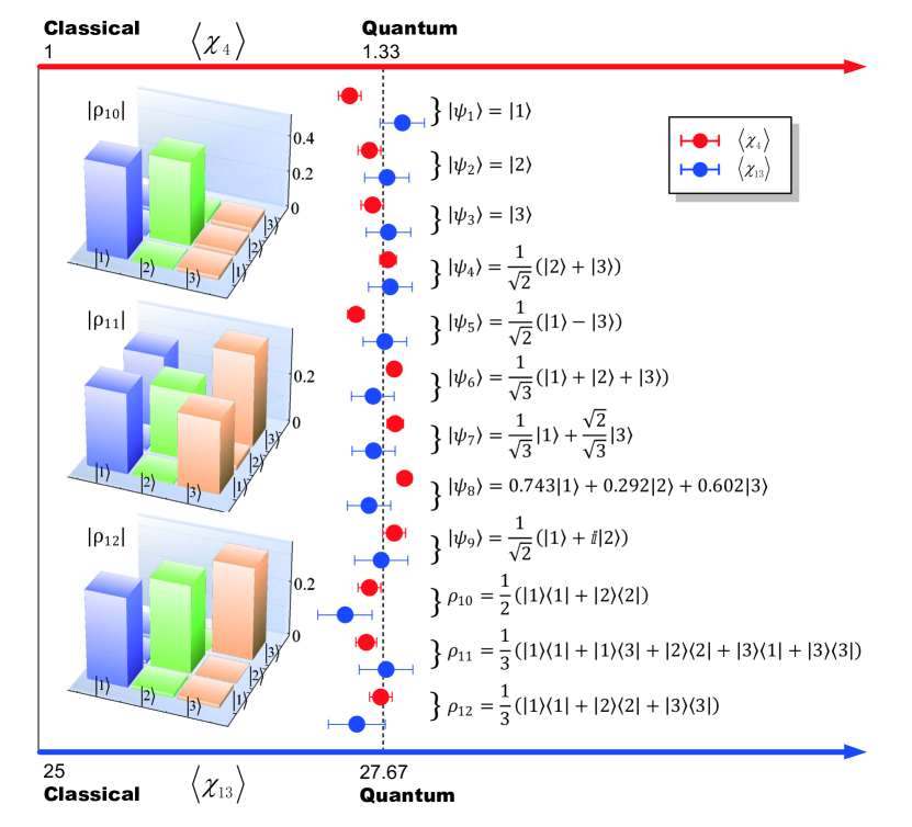
Figure 3: State-independent test of KS inequalities χ4delimited-⟨⟩subscript𝜒4\left\langle\chi_{4}\right\rangle and χ13delimited-⟨⟩subscript𝜒13\left\langle\chi_{13}\right\rangle for a qutrit system. The inequalities (1) and (2) are examined with eleven different initial states including simple product states ψ1subscript𝜓1\psi_{1} to ψ3subscript𝜓3\psi_{3}, superposition states at the axis of the observables ψ4subscript𝜓4\psi_{4} to ψ6subscript𝜓6\psi_{6}, outside of the observables ψ7subscript𝜓7\psi_{7} to ψ9subscript𝜓9\psi_{9}, and mixed states ψ10subscript𝜓10\psi_{10} to ψ12subscript𝜓12\psi_{12}. We measure the density matrix of all states by performing qutrit state tomography Thew et al. (2002) and confirm the prepared states with an average fidelity 99.5%percent99.599.5\% for the pure states ψ1subscript𝜓1\psi_{1} to ψ9subscript𝜓9\psi_{9}. The mixed state fidelities are around 97%percent9797\% shown in the figure. All raw measurements for χ13delimited-⟨⟩subscript𝜒13\left\langle\chi_{13}\right\rangle shown as blue filled circles violate the classical limit 25 by 15σ15𝜎15\sigma, confirming the quantum contextuality for various states. For each states, 480,000 realizations are used to obtain the χ13delimited-⟨⟩subscript𝜒13\left\langle\chi_{13}\right\rangle. For the inequality (2), the average value of all measured initial states is χ4=1.328(11)delimited-⟨⟩subscript𝜒41.32811\left\langle\chi_{4}\right\rangle=1.328(11).

The procedures of our experiments are as follows: after 1 ms Doppler cooling, the state of the ion is initialized to |3ket3\left|3\right\rangle by 3 μ𝜇\mus standard optical pumping Olmschenk et al. (2007). The states are coherently manipulated by the microwaves ω1subscript𝜔1\omega_{1} and ω2subscript𝜔2\omega_{2} that are resonant to the transitions between |1ket1\left|1\right\rangle and |3ket3\left|3\right\rangle, and between |2ket2\left|2\right\rangle and |3ket3\left|3\right\rangle, respectively. The 2 π𝜋\pi times for both Rabi oscillations are adjusted to 29.5 μ𝜇\mus, that is Ω1,2=(2π) 33.9subscriptΩ122𝜋33.9\Omega_{1,2}=(2\pi)\leavevmode\nobreak\ 33.9 kHz in frequency. The separation ω2ω1subscript𝜔2subscript𝜔1\omega_{2}-\omega_{1} = (2π)2𝜋(2\pi) 7.6372 MHz with the magnetic field B𝐵B= 5.455 G, which is large enough to ensure the independency of each Rabi oscillation.

The 24 correlations of 13 observables of a given initial state are measured after rotating the observables on the one of qutrit states, shown in Table 1. We prepare the measurement settings to map at least two orthogonal observables on the measurement basis simultaneously. The probabilities of |1ket1\left|1\right\rangle and |2ket2\left|2\right\rangle are obtained by mapping each state onto |3ket3\left|3\right\rangle and measuring the probability of |3ket3\left|3\right\rangle. We repeat the same measurements 10,000 times for the same observables, which result in 480,000 repetitions for one initial state. After obtaining all the results of measurements, we apply the detection-error correction scheme with the maximally likelyhood method Shen and Duan (2012). The state detection errors of no-photon state, |3ket3\left|3\right\rangle and of not detecting the |3ket3\left|3\right\rangle states are 1.0%percent1.01.0\% and 2.1%percent2.12.1\%, respectively, with the discrimination threshold nph=1subscript𝑛𝑝1n_{ph}=1 shown in Fig. 2(b).

We examine the state-independency of the inequalities (1) and (2) by preparing eleven different initial states shown in Fig. 3 and repeating the measurements described in Table 1. We verify that both inequalities are violated for simple input states ψ1subscript𝜓1\psi_{1} to ψ3subscript𝜓3\psi_{3}, superposition states aligning to one of 13 observables ψ4subscript𝜓4\psi_{4} to ψ6subscript𝜓6\psi_{6}, general superposition states not related to measurement axes ψ7subscript𝜓7\psi_{7} to ψ9subscript𝜓9\psi_{9}, mixed states ρ10subscript𝜌10\rho_{10} to ρ12subscript𝜌12\rho_{12}. The pulse sequences and state-tomography results are presented in the supplementary information. We observe the fidelities of the prepared states on average 99.5 %percent\% for the pure states.

We clearly observe the violations of the inequaliteis (1) and (2) for all the input states that we prepared, including mixed states as summarized in Fig. 3. The average of χ13=27.63(17)delimited-⟨⟩subscript𝜒1327.6317\left\langle\chi_{13}\right\rangle=27.63(17) and χ4=1.328(11)delimited-⟨⟩subscript𝜒41.32811\left\langle\chi_{4}\right\rangle=1.328(11), significantly larger than the limits of non-contextual models. For some of input states, χ4delimited-⟨⟩subscript𝜒4\left\langle\chi_{4}\right\rangle and χ13delimited-⟨⟩subscript𝜒13\left\langle\chi_{13}\right\rangle are even larger than quantum bounds. However, the breaking of quantum bounds does not have serious meaning, since the results are within uncertainties of the measurements. We also observe the violations for all the states even without the correction of detection errors. However, the some of results are unphysical and violating even the quantum limit simply because of the detection errors. We provide all the detailed measurement results with and without detection error corrections in the supplementary information.

In conclusion, our results show experimental measurements of an simplest three-level quantum system in an indivisible single atomic ion, which are incompatible to any non-contextual models. The results confirms the quantum contextuality for any states in three dimensions without entanglements or even superposition. Our experimental violations are not subject to the detection loophole. However, the sequencial measurements open the compatibility loophole Gühne et al. (2010). In our particular measurements, most of the observables in the inequalities are individual, which is irrelevant to the compatibilty loophole. And the correlations would be ignored if we require the same compatible algebric structure on the hidden variable models. Particularly, the violations of χ4delimited-⟨⟩subscript𝜒4\left\langle\chi_{4}\right\rangle conclude the quantum contextuality without detection and compatiblity loopholes.

.1 Acknowledgement

We thank Hyunchul Nha and Sewan Ji for the helpful discussion. We thank Emimly Lichko for carefully reading and improving the manuscript. This work was supported in part by the National Basic Research Program of China Grant 2011CBA00300, 2011CBA00301, 2011CBA00302, the National Natural Science Foundation of China Grant 61073174, 61033001, 61061130540. KK acknowledges the support from the Thousand Young Talents program.

References

  • Kochen and Specker (1967) S. Kochen and E. P. Specker, J. Math. Mech. 17, 59 (1967).
  • Bell (1966) J. S. Bell, Rev. Mod. Phys. 38, 447 (1966).
  • Mermin (1990) N. D. Mermin, Phys. Rev. Lett. 65, 3373 (1990).
  • Peres (1991) A. Peres, J. Phys. A 24, L175 (1991).
  • Cabello (2008) A. Cabello, Phys. Rev. Lett. 101, 210401 (2008).
  • Michler et al. (2000) M. Michler, H. Weinfurter, and M. Żukowski, Phys. Rev. Lett. 84, 5457 (2000).
  • Huang et al. (2003) Y.-F. Huang, C.-F. Li, Y.-S. Zhang, J.-W. Pan, and G.-C. Guo, Phys. Rev. Lett. 90, 250401 (2003).
  • Bartosik et al. (2009) H. Bartosik, J. Klepp, C. Schmitzer, S. Sponar, A. Cabello, H. Rauch, and Y. Hasegawa, Phys. Rev. Lett. 103, 040403 (2009).
  • Kirchmair et al. (2009) G. Kirchmair, F. Zähringer, R. Gerritsma, M. Kleinmann, O. Gühne, A. Cabello, R. Blatt, and C. F. Roos, Nature 460, 494 (2009).
  • Amselem et al. (2009) E. Amselem, M. Rådmark, M. Bourennane, and A. Cabello, Phys. Rev. Lett. 103, 160405 (2009).
  • Moussa et al. (2010) O. Moussa, C. A. Ryan, D. G. Cory, and R. Laflamme, Phys. Rev. Lett. 104, 160501 (2010).
  • Klyachko et al. (2008) A. A. Klyachko, M. A. Can, S. Binicioğlu, and A. S. Shumovsky, Phys. Rev. Lett. 101, 020403 (2008).
  • Lapkiewicz et al. (2011) R. Lapkiewicz, P. Li, C. Schaeff, N. K. Langford, S. Ramelow, M. Wieśniak, and A. Zeilinger, Nature 474, 490 (2011).
  • Yu and Oh (2012) S. Yu and C. H. Oh, Phys. Rev. Lett. 108, 020403 (2012).
  • Cabello et al. (2012) A. Cabello, C. Budroni, O. Gühne, M. Kleinmann, and J. Åke Larsson, arXiv:1204.3741 (2012).
  • Zu et al. (2012) C. Zu, Y.-X. Wang, D.-L. Deng, X.-Y. Chang, K. Liu, P.-Y. Hou, H.-X. Yang, and L.-M. Duan, arXiv:1207.0059 (2012).
  • Cabello (2011) A. Cabello, arXiv:1112.5149 (2011).
  • Olmschenk et al. (2007) S. Olmschenk, K. C. Younge, D. L. Moehring, D. N. Matsukevich, P. Maunz, and C. Monroe, Phys. Rev. A 76, 052314 (2007).
  • Liebfried et al. (2003) D. Liebfried, R. Blatt, C. Monroe, and D. Wineland, Rev. Mod. Phys. 75, 281 (2003).
  • Häffner et al. (2008) H. Häffner, C. F. Roos, and R. Blatt, Phys. Rep. 469 (2008).
  • Acton (2008) M. Acton, Ph.D. thesis, University of Michigan, Ann Arbor (2008).
  • Brown et al. (2011) K. R. Brown, A. C. Wilson, Y. Colombe, C. Ospelkaus, A. M. Meier, E. Knill, D. Leibfried, and D. J. Wineland, Phys. Rev. A 84, 030303(R) (2011).
  • Thew et al. (2002) R. T. Thew, K. Nemoto, A. G. White, and W. J. Munro, Phys. Rev. A 66, 012303 (2002).
  • Shen and Duan (2012) C. Shen and L. M. Duan, New J. Phys. 14, 053053 (2012).
  • Gühne et al. (2010) O. Gühne, M. Kleinmann, A. Cabello, J. Åke Larsson, G. Kirchmair, F. Zähringer, R. Gerritsma, and C. F. Roos, Phys. Rev. A 81, 022121 (2010).