Minimal realization of the dynamical structure function and its application to network reconstruction

Abstract

Network reconstruction, i.e., obtaining network structure from data, is a central theme in systems biology, economics and engineering. In some previous work, we introduced dynamical structure functions as a tool for posing and solving the problem of network reconstruction between measured states. While recovering the network structure between hidden states is not possible since they are not measured, in many situations it is important to estimate the minimal number of hidden states in order to understand the complexity of the network under investigation and help identify potential targets for measurements. Estimating the minimal number of hidden states is also crucial to obtain the simplest state-space model that captures the network structure and is coherent with the measured data. This paper characterizes minimal order state-space realizations that are consistent with a given dynamical structure function by exploring properties of dynamical structure functions and developing an algorithm to explicitly obtain such a minimal realization.

I Introduction

Networks have received an increasing amount of attention in the last decade. In our “information-rich” world, the questions of network reconstruction and network analysis become crucial for the understanding of complex systems such as biological, social, or economical networks. In particular, the analysis of molecular networks has gained significant interest due to the recent explosion of publicly available high-throughput biological data. In this context, the question of identifying and analyzing the network structure at the origin of measured data becomes a key issue.

In some occasions, measured data is given in the form of input-output time-series that describes the effect of inputs on outputs (measured states) of a network. When data is generated by a linear system, a matrix transfer function describing the dynamic input-output behavior is generally obtained using system identification [1]. If the original state-space model is available or deducible, then the associated network structure can be readily obtained from it. However, a transfer function cannot, in general, recover, or realize, the original state-space model since the realization problem does not typically have a unique solution, i.e., different state-space realizations can generate the same input-output behavior. Since each of these realizations may suggest entirely different network structures, it is in general impossible to identify network structures from transfer functions alone. Therefore, more information, beyond input-output data used to identify a transfer function, is needed to prefer one state-space realization over another as a description of a particular system[2].

Another difficulty in the network reconstruction problem comes from the fact that the realization problem becomes ill posed when some of the states are unobservable or “hidden” (this happens with just one hidden state [3, pp. $78$]). As a result, failure to explicitly acknowledge the presence of hidden states and the resulting ambiguity in network structures can lead to a deceptive and erroneous process for network structure discovery. Consequently, determining from measured data the presence or absence of a causal relationship between two variables in a network is a challenging question.

Motivated by this, we are focusing on the effect of hidden states in the network that we are aiming to reconstruct. A new representation for LTI systems, called dynamical structure functions was introduced in [4] and developed in [5, 6, 7, 8, 9, 10] . Dynamical structure functions capture information at an intermediate level between transfer function and state space representation (see Figure 1). Specifically, dynamical structure functions not only encode structural information at the measurement level, but also contain some information about hidden states. Based on the theoretical results presented in [4], we proposed some guidelines for the design of an experimental data-acquisition protocol which allows the collection of data containing sufficient information for the network structure reconstruction problem to become solvable. In particular, we have shown that if nothing is known about the network, then reconstruction is impossible. If, however, one can make the following reasonable assumptions about the data-collection experiments: Networks have received an increasing amount of attention in the last decade. In our “information-rich” world, the questions of network reconstruction and network analysis become crucial for the understanding of complex systems such as biological, social, or economical networks. In particular, the analysis of molecular networks has gained significant interest due to the recent explosion of publicly available high-throughput biological data. In this context, the question of identifying and analyzing the network structure at the origin of measured data becomes a key issue.

In some occasions, measured data is given in the form of input-output time-series that describes the effect of inputs on outputs (measured states) of a network. When data is generated by a linear system, a matrix transfer function describing the dynamic input-output behavior is generally obtained using system identification [1]. If the original state-space model is available or deducible, then the associated network structure can be readily obtained from it. However, a transfer function cannot, in general, recover, or realize, the original state-space model since the realization problem does not typically have a unique solution, i.e., different state-space realizations can generate the same input-output behavior. Since each of these realizations may suggest entirely different network structures, it is in general impossible to identify network structures from transfer functions alone. Therefore, more information, beyond input-output data used to identify a transfer function, is needed to prefer one state-space realization over another as a description of a particular system[2].

Another difficulty in the network reconstruction problem comes from the fact that the realization problem becomes ill posed when some of the states are unobservable or “hidden” (this happens with just one hidden state [3, pp. $78$]). As a result, failure to explicitly acknowledge the presence of hidden states and the resulting ambiguity in network structures can lead to a deceptive and erroneous process for network structure discovery. Consequently, determining from measured data the presence or absence of a causal relationship between two variables in a network is a challenging question.

Motivated by this, we are focusing on the effect of hidden states in the network that we are aiming to reconstruct. A new representation for LTI systems, called dynamical structure functions was introduced in [4] and developed in [5, 6, 7, 8, 9, 10] . Dynamical structure functions capture information at an intermediate level between transfer function and state space representation (see Figure 1). Specifically, dynamical structure functions not only encode structural information at the measurement level, but also contain some information about hidden states. Based on the theoretical results presented in [4], we proposed some guidelines for the design of an experimental data-acquisition protocol which allows the collection of data containing sufficient information for the network structure reconstruction problem to become solvable. In particular, we have shown that if nothing is known about the network, then reconstruction is impossible. If, however, one can make the following reasonable assumptions about the data-collection experiments:

1. for a network composed of $p$ measured species, the same number of experiments $p$ must be performed;

2. each experiment must independently control a measured species, i.e., control input $i$ must first affect measured species $i$,

then reconstruction is possible. Moreover, failure to meet the necessary informativity conditions results in a situation where any internal network structure fits the data equally well (e.g. a fully decoupled network or a fully connected network). If biologists have already some information about the network, as it is usually the case, then these conditions can be relaxed as explained in [4]. Using dynamical structure functions as a mean to solve the network reconstruction problem, the following aspects need to be considered (see Figure 1):

Figure 1: Mathematical structure of the network reconstruction problem using dynamical structure functions. Red arrows mean “uniquely determine”, blue arrows indicate our work.

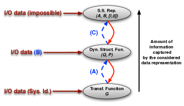
First (see (A) in Figure 1), the properties of a dynamical structure function and its relationship with the transfer function associated with the same system need to be precisely established (this was done in [4]).

Second (see (B) in Figure 1), an efficient method is developed to reconstruct networks in the presence of noise and nonlinearities (this was done in [11]). This method relies on the assumption that the conditions for network reconstruction presented above in (A.1) and (A.2) have been met. In our approach, we use the same information as traditional system identification methods, i.e., input-output data. However, with our method, steady-state (resp. time-series data) can be used to reconstruct the Boolean (resp. dynamical network) structure of the system (see [11] for more details).

Third (see (C) in Figure 1), once the dynamical structure function is obtained, as a main result of this paper, an algorithm for constructing a minimal order state-space representation consistent with such function is developed. In an application, this provides a way to estimate the complexity of the system by determining the minimal number of hidden states in the system. For example, in the context of biology it helps understand the number of unmeasured molecules in a particular pathway: a low number means that most molecules in that pathway have been identified and measured, showing a good understanding of the system; while a large number shows that there are still many unmeasured variables, suggesting that new experiments should be carried out to better characterize that pathway.

The outline of the paper is as follows. Section II reviews the definition of dynamical structure functions and their properties. The main result can be found in Section III where we propose a minimal order realization algorithm based on state-space realizations and pole-zero analysis. Simulation and discussion are addressed in Section IV. Finally conclusions are presented in Section V.

II System Model

Consider a linear system (it can also be a linearization of some original nonlinear system) $\dot{{x}}={Ax}+{Bu}$, ${y}={Cx}$. The transfer function associated with this system is given by ${G(s)}={C}(s{I}-{A})^{-1}{B}$. Typically, we can use standard system identification tools [1] to identify a transfer function ${G(s)}$ from input-output data.

Like system realization, network reconstruction also begins with the identification of a transfer function, but it additionally attempts to determine the network structure between measured states without imposing any additional structure on the hidden states. As we have shown in [4], this requires a new representation of linear time-invariant systems: the dynamical structure function (defined later). An algorithm allowing the dynamical structure function to be obtained from input-output data is proposed in [11]. This paper assumes that the dynamical structure function has already been obtained from data, and will focus on finding one of its minimal state-space realizations.

The dynamical structure function is obtained as follows: First, we transform $[{A},{B},{C}]$ to $\left[{A}^{o},{B}^{o},\begin{bmatrix}{I}_{p}&{0}\end{bmatrix}\right]$ without changing $G(s)$, where $p=\text{rank}(C)$. The linear system dynamics then writes

$$\begin{array}[]{cll}\left[\begin{array}[]{c}{\dot{y}}\\ {\dot{z}}\end{array}\right]&=&\left[\begin{array}[]{cc}{A}^{o}_{11}&{A}^{o}_{12}\\ {A}^{o}_{21}&{A}^{o}_{22}\end{array}\right]\left[\begin{array}[]{c}{y}\\ {z}\end{array}\right]+\left[\begin{array}[]{c}{B}^{o}_{1}\\ {B}^{o}_{2}\end{array}\right]{u}\\ {y}&=&\left[\begin{array}[]{cc}{I}_{p}&{0}\end{array}\right]\left[\begin{array}[]{c}{y}\\ {z}\end{array}\right]\end{array}$$ (1)

where ${x}=({y},{z})\in\mathbb{R}^{n^{o}}$ is the full state vector, ${y}\in\mathbb{R}^{p}$ is a partial measurement of the state, ${z}$ are the $n^{o}-p$ “hidden” states, and ${u}\in\mathbb{R}^{m}$ is the control input. In this work we restrict our attention to situations where output measurements constitute partial state information, i.e., $p<n^{o}$. We consider only systems with full rank transfer functions that do not have entire rows or columns of zeros, since such “disconnected” systems are somewhat pathological and only serve to complicate the exposition without fundamentally altering our conclusions.

Taking the Laplace transforms of the signals in (1) yields

$$\begin{array}[]{lll}\left[\begin{array}[]{c}s{Y}\\ s{Z}\end{array}\right]&=&\left[\begin{array}[]{cc}{A}^{o}_{11}&{A}^{o}_{12}\\ {A}^{o}_{21}&{A}^{o}_{22}\end{array}\right]\left[\begin{array}[]{c}{Y}\\ {Z}\end{array}\right]+\left[\begin{array}[]{c}{B}^{o}_{1}\\ {B}^{o}_{2}\end{array}\right]{U}\end{array}$$ (2)

where ${Y}$, ${Z}$, and ${U}$ are the Laplace transforms of ${y}$, ${z}$, and ${u}$, respectively. Solving for ${Z}$ gives

$${Z}=\left(s{I}-{A}^{o}_{22}\right)^{-1}{A}^{o}_{21}{Y}+\left(s{I}-{A}^{o}_{22}\right)^{-1}{B}^{o}_{2}{U}$$

Substituting this last expression of ${Z}$ into (2) then yields

$$s{Y}={W}^{o}{Y}+{V}^{o}{U}$$ (3)

where ${W}^{o}={A}^{o}_{11}+{A}^{o}_{12}\left(s{I}-{A}^{o}_{22}\right)^{-1}{A}^{o}_{21}$ and ${V}^{o}={B}^{o}_{1}+{A}^{o}_{12}\left(s{I}-{A}^{o}_{22}\right)^{-1}{B}^{o}_{2}$.

Now, let ${R}^{o}$ be a diagonal matrix formed of the diagonal terms of ${W}^{o}$ on its diagonal, i.e., ${R}^{o}=\mbox{diag}\{{W}^{o}\}=\mbox{diag}(W^{o}_{11},W^{o}_{22},...,W^{o}_{pp})$. Subtracting ${R}^{o}{Y}$ from both sides of (3), we obtain:

$$\left(s{I}-{R}^{o}\right){Y}=\left({W}^{o}-{R}^{o}\right){Y}+{V}^{o}{U}$$

Note that ${W}^{o}-{R}^{o}$ is a matrix with zeros on its diagonal. We thus have:

$${Y}={QY}+{PU}$$ (4)

where

$${Q}=\left(s{I}-{R}^{o}\right)^{-1}\left({W}^{o}-{R}^{o}\right)$$ (5)

and

$${P}=\left(s{I}-{R}^{o}\right)^{-1}{V}^{o}$$ (6)

Note that ${Q}$ is zero on the diagonal.

Definition 1

Given the system (1), we define the dynamical structure function of the system to be $[{Q},{P}]$.

Note that, in general, ${Q(s)}$ and ${P(s)}$ carry a lot more information than ${G(s)}$. This can be seen from the equality ${G}(s)=({I}-{Q}(s))^{-1}{P}(s)$ (see [4] for details). However, ${Q(s)}$ and ${P(s)}$ carry less information than the state-space model (1) (see [11]).

Definition 2

A dynamical structure function, $[{Q},{P}]$, is said to be consistent with a particular transfer function, ${G}$, if there exists a realization of ${G}$, of some order, and of the form (1), such that $[{Q},{P}]$ are specified by (5) and (6). Likewise, a realization is consistent with $[{Q},{P}]$ if that realization gives $[{Q},{P}]$ from (5) and (6).

Definition 3

We say that a realization is ${G}$ minimal if this realization corresponds to a minimal realization of ${G}$. We say that a realization is $[{Q},{P}]$ minimal if this realization is consistent with $[{Q},{P}]$ and its order is smaller than or equal to that of all realizations consistent with $[{Q},{P}]$.

The underlying principle to find a $[{Q},{P}]$ minimal realization is to search for a realization with the minimal number of hidden states. Such a realization is characterized by the minimal number of pole-zero cancellations in the transfer functions ${Q}$ and ${P}$.

Proposition 1

Given a dynamical system (1) and the associated dynamical structure functions $[{Q},{P}]$ with ${R}^{o}$ constructed as explained above (see (1)-(6)), the following conditions must hold

$$\text{diag}\{{A}^{o}_{11}\} =\lim_{s\rightarrow\infty}{R}^{o}(s);$$ (7)

$${A}^{o}_{11}-\text{diag}\{{A}^{o}_{11}\} =\lim_{s\rightarrow\infty}s{Q}(s);$$ (8)

$${B}^{o}_{1} =\lim_{s\rightarrow\infty}s{P}(s).$$ (9)

Proof:

Eq. (7) is directly obtained from the definition of ${R}^{o}(s)$:

$$\lim_{s\rightarrow\infty}{R}^{o}(s) =\lim_{s\rightarrow\infty}\text{diag}\{{W}^{o}(s)\}$$

$$=\text{diag}\{\lim_{s\rightarrow\infty}{W}^{o}(s)\}=\text{diag}\{{A}_{11}^{o}\}$$

Since the proofs for eq. (8) and (9) are very similar, we focus on eq. (8) only. Using the fact that for any square matrix ${M}$, if $M^{n}\rightarrow 0$ when $n\rightarrow+\infty$, then $({I}-{M})^{-1}=\sum_{i=0}^{\infty}{M}^{i}$, we obtain, from the definition of ${Q}$ given in (5), ${Q}(s)=\sum_{i=1}^{\infty}s^{-i}{R}^{o~{}i-1}(s)\left({W}^{o}(s)-{R}^{o}(s)\right)$ and ${W}^{o}(s)={A}^{o}_{11}+\sum_{i=1}^{\infty}s^{-i}{A}^{o}_{12}{A}_{22}^{o~{}i-1}{A}^{o}_{21}$, when $s\rightarrow+\infty$. Hence, ${Q}(s)=({A}^{o}_{11}-{R}^{o}(s))s^{-1}+{r}(s)$, in which ${r}(s)$ is a matrix polynomial of $s$, whose largest degree is $-2$. Finally, multiplying by $s$ on both sides and taking the limit as $s$ goes to $\infty$ results in eq. (8). A similar argument can be used to prove eq. (9). ∎

Remark 1

This Proposition reveals an important property of dynamical structure functions: they encode the direct causal relationships between observed variables.

We present hereafter an illustrative example to help fix the ideas.

Example 1

Consider a network with the structure depicted in Fig. 2. A linear state-space representation of this network is given by

$$\begin{array}[]{rcl}\dot{x}&=&\begin{bmatrix}a_{11}&0&a_{13}&0&0\\ 0&a_{22}&0&a_{24}&0\\ 0&a_{32}&a_{33}&0&a_{35}\\ a_{41}&0&0&a_{44}&0\\ 0&a_{52}&0&0&a_{55}\end{bmatrix}x+\begin{bmatrix}b_{11}&0\\ 0&b_{22}\\ 0&0\\ 0&0\\ 0&0\end{bmatrix}u\\ y&=&\begin{bmatrix}I_{3}&0\end{bmatrix}x\end{array}$$

where $I_{3}$ is the $3\times 3$ identity matrix. Following the definitions in (5) and (6), we can write down the corresponding dynamical structure function $[{Q},{P}]$ as

$$Q =\begin{pmatrix}0&0&\frac{a_{13}}{s-a_{11}}\\ \frac{a_{24}a_{41}}{(s-a_{22})(s-a_{44})}&0&0\\ 0&\frac{a_{35}a_{52}+a_{32}(s-a_{55})}{(s-a_{33})(s-a_{55})}&0\end{pmatrix},$$

$$P =\begin{pmatrix}\frac{b_{11}}{s-a_{11}}&0\\ 0&\frac{b_{22}}{s-a_{22}}\\ 0&0\end{pmatrix}.$$

Figure 2: (a) An example system with two inputs, three measured states (states $1$, $2$, and $3$) and two hidden states (states $4$ and $5$). (b) The corresponding dynamical network structure.

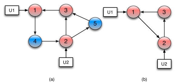
Consistent with Proposition 1, we can check using the above that:

$$\lim_{s\rightarrow\infty}s{Q}(s) =\begin{pmatrix}0&0&a_{13}\\ 0&0&0\\ 0&a_{32}&0\end{pmatrix};$$

$$\lim_{s\rightarrow\infty}s{P}(s) =s\begin{pmatrix}\frac{b_{11}}{s-a_{11}}&0\\ 0&\frac{b_{22}}{s-a_{22}}\\ 0&0\end{pmatrix}=\begin{pmatrix}b_{11}&0\\ 0&b_{22}\\ 0&0\end{pmatrix}.$$

Generally, there exist many realizations consistent with $[{Q},{P}]$. In the following section, we focus on finding a $[{Q},{P}]$ minimal realization $\left(A,B,\begin{bmatrix}I&0\end{bmatrix}\right)$, i.e., a realization which is consistent with $[{Q},{P}]$ and which has minimal order, that is, with minimal dimension for $A$ (and hence the lowest possible complexity).

III Algorithm to find a $[{Q},{P}]$ minimal realization

From a dynamical structure function $[{Q},{P}]$ we cannot reconstruct $[{W}^{o},{V}^{o}]$ since there is no information regarding the diagonal transfer function matrix ${R}^{o}$. Given $[{Q},{P}]$ and a diagonal proper transfer function matrix ${R}$, a minimal realization of $[{W}~{}~{}{V}]=[(s{I}-{R}){Q}+{R}~{}~{}(s{I}-{R}){P}]$ can be obtained as follows. We know that:

$$[{W}~{}~{}{V}]=[{A}_{11}~{}~{}{B}_{1}]+{A}_{12}(s{I}-{A}_{22})^{-1}[{A}_{21}~{}~{}{B}_{2}]$$ (10)

The idea is to start with an arbitrarily chosen ${R}$, and then use a state-space realization approach to find a ${R}^{*}$ which minimizes the order of a minimal realization of $[{W}~{}~{}{V}]$.

Lemma 1

Suppose ${W}$, ${V}$, ${A}=\begin{bmatrix}A_{11}&A_{12}\\ A_{21}&A_{22}\end{bmatrix}$ and ${B}=\begin{bmatrix}B_{1}\\ B_{2}\end{bmatrix}$ are defined as in eq. (10), then ${V}$ and ${G}$ share the same zeros.

Proof:

Since $s{I}-{W}$ is the Schur complement of $s{I}-{A}_{22}$ in $s{I}-{A}$, then

$$\det(s{I}-{W})=\frac{\det(s{I}-{A})}{\det(s{I}-{A}_{22})}.$$ (11)

Recall that ${V}={B}_{1}+{A}_{12}(s{I}-{A}_{22})^{-1}{B}_{2}$. Since $(s{I}-{W}){G}={V}$, we thus have that ${V}$ and ${G}$ share the same zeros [15, page $153$]. ∎

Given a dynamical structure function $[{Q},{P}]$, a random choice of a proper diagonal transfer function matrix ${R}$ is likely to result in additional zeros in ${V}=(s{I}-{R}){P}$. From Lemma 1, this will lead to additional zeros in ${G}$ which are associated to uncontrollable eigenvalues of the considered realization [12, Section 4] and of course does not lead to a minimal realization in eq. (10). At this stage the following question arises: how can we find a proper diagonal transfer function matrix ${R}^{*}$ such that a minimal realization of $[{W}~{}~{}{V}]$ is a $[{Q},{P}]$ minimal realization, i.e.,

$$R^{*}=\textbf{argmin}_{R}~{}\text{deg}\left\{(s{I}-{R})s^{-1}[s{Q}~{}~{}s{P}]+[{R}~{}~{}{0}]\right\},$$ (12)

where deg is the McMillan degree [3]. Note that, since there are many choices for ${R}^{*}$ that minimize the order of minimal realizations of $[{W}~{}~{}{V}]$, a chosen ${R}^{*}$ may be different from ${R}^{o}$.

Assume that all elements in $[{Q}~{}~{}{P}]$ only have simple poles. This assumption can be relaxed but we adopt it here for simplicity. Also assume that $[{Q}~{}~{}{P}]$ does not possess any poles at $0$ (otherwise we can change eq. (12) to $(s{I}-{R})(s-a)^{-1}[(s-a){Q}~{}~{}(s-a){P}]+[{R}~{}~{}{0}]$, where $a\in\mathbb{R}$ is not a pole of $[{Q}~{}~{}{P}]$).

Proposition 2

Assume $[{I-Q}~{}~{}{P}]$ only has simple poles and does not have any zeros. A minimal order realization of $[{W}~{}~{}{V}]$ in (10) can be achieved using a constant diagonal matrix ${R}^{*}$.

Proof:

Assume ${R}^{*}$ has at least one term on the diagonal with the degree of the numerator greater or equal to $1$, e.g., suppose the $i^{th}$ term in $(s{I}-{R}^{*})s^{-1}=\frac{(s+b)\epsilon_{i}(s)}{s\phi_{i}(s)}$ with any $b\in\mathbb{R}$ and $deg(\epsilon_{i}(s))=deg(\phi_{i}(s))\geq 1$, where $deg(\cdot)$ returns the degree of a polynomial. Hence, the product $(s{I}-{R}^{*})s^{-1}[s{Q}~{}~{}s{P}]$ will introduce $deg(\phi_{i}(s))$ new poles and, due the assumption of simple poles, can at most eliminate $deg(\epsilon_{i}(s))=deg(\phi_{i}(s))$ poles since $[{I-Q}~{}~{}{P}]$ does not have any zeros. As a consequence, we can change the $i^{th}$ term from $\frac{(s+b)\epsilon_{i}(s)}{s\phi_{i}(s)}$ to $\frac{s+a}{s}$ without increasing the order. Doing this along all the elements of ${R}^{*}$ proves the result. ∎

If ${R}^{*}$ is a constant matrix, the term $[{R}^{*}~{}~{}{0}]$ in eq. (12) is also a constant matrix. Therefore, the order of a minimal realization is only determined by $(s{I}-{R}^{*})s^{-1}[s{Q}~{}~{}s{P}]\triangleq{N}[s{Q}~{}~{}s{P}]$. Thus, finding the “optimal” ${R}^{*}$ which leads to the minimal order in eq. (12) is equivalent to finding a diagonal proper transfer matrix ${N}$ such that ${N}[s{Q}~{}~{}s{P}]$ has as few poles as possible. Based on this idea, the following algorithm is proposed:

Step 1: Find a Gilbert’s realization of the dynamical structure function.
First, using the results in [4, Lemma 1], we find a minimal realization $({A}_{1},{B}_{1},{C}_{1},{D}_{1})$ of $[s{Q}~{}~{}s{P}]$. When $[s{Q}~{}~{}s{P}]$ has $l$ simple poles, using Gilbert’s realization [13] gives

$$[s{Q}~{}~{}s{P}]=\sum_{i=1}^{l}\frac{{K}_{i}}{s-\lambda_{i}}+\lim_{s\rightarrow\infty}[s{Q}~{}~{}s{P}],$$

where ${K}_{i}=\lim_{s\rightarrow\lambda_{i}}(s-\lambda_{i})[s{Q}~{}~{}s{P}]$ and has rank $1$ since we are assuming that $[s{Q}~{}~{}s{P}]$ has simple poles.

Consider a matrix decomposition of ${K}_{i}$ of the following form:

$${K}_{i}={E}_{i}{F}_{i},~{}\forall i,$$

where ${E}_{i}\in\mathbb{R}^{p}$ and ${F}_{i}=({E}_{i}^{T}{E}_{i})^{-1}{E}_{i}^{T}{K}_{i}$. Then ${A}_{1}=\text{diag}\{\lambda_{i}\}\in\mathbb{R}^{l\times l}$, ${B}_{1}=\begin{bmatrix}{F}^{T}_{1}&{F}^{T}_{2}&\ldots&{F}^{T}_{l}\end{bmatrix}^{T}$, ${C}_{1}=\begin{bmatrix}{E}_{1}&{E}_{2}&\ldots&{E}_{l}\end{bmatrix}$ and ${D}_{1}=\lim_{s\rightarrow\infty}[s{Q}~{}~{}s{P}]$.

Step 2: Find the maximal number of cancelled poles.
We define $\Phi$ as a largest subset of $\{{E}_{1},\cdots,{E}_{l}\}$ such that all the elements in $\Phi$ are mutually orthogonal. We also define $\phi$ as the cardinality of $\Phi$. Computationally, $\phi$ can be obtained using the algorithm presented in the Appendix. We claim that $\phi$ is equal to the maximum number of poles we can eliminate (the proof is in the Appendix). Therefore, the minimal order of $[{W}~{}~{}{V}]$ is

$$l-\phi.$$

As a consequence, the order of the minimal reconstruction is the dimension of ${A}_{11}$ (the constant $p$) plus the minimal dimension of ${A}_{22}$ (obtained above): $p+l-\phi$.

Step 3: Construct ${R}^{*}$ to obtain the minimal reconstruction.
Once we have $\Phi$, using eq. (13) and ${R}^{*}=s{I}-s{N}$, we know that ${N}(\lambda_{i})[j,j]=0$ implies ${R}^{*}[j,j]=\lambda_{i}$. Consequently, each element in the set $\Phi$ will determine at least one element in ${R}^{*}$. This last fact can be used to construct ${R}^{*}$ element by element. Once ${R}^{*}$ is found, we can obtain ${A}$ and ${B}$ using eq. (10).

IV Illustrative example

Example 2

Consider a dynamical structure function $[{Q},{P}]$:

$$[{Q}\ |\ {P}]=\begin{bmatrix}0&\frac{1}{s+2}&\frac{1}{s+3}&|&\frac{1}{s+4}\\ \frac{1}{s+1}&0&\frac{1}{s+3}&|&\frac{1}{s+4}\\ \frac{1}{s+1}&\frac{1}{s+2}&0&|&\frac{1}{s+4}\end{bmatrix}.$$

We first compute the McMillan degree of the corresponding transfer function: $\text{deg}\{G\}=\text{deg}\{(I-Q)^{-1}P)\}=4$, meaning that a $4^{th}$ order state-space model is enough to realize the transfer function. It is interesting to look at the minimal order realization consistent with the dynamical structure function. The different steps of the algorithm proposed in the previous section successively yield the following:

Step 1: A minimal Gilbert realization of $s[{Q},{P}]$ is

$${A}_{1}=\text{diag}\{-1,-2,-3,-4\},~{}{B}_{1}=\text{diag}\{2,2,2,4\},$$

$${C}_{1}=\begin{bmatrix}0&-1&-1.5&-1\\ -0.5&0&-1.5&-1\\ -0.5&-1&0&-1\end{bmatrix},~{}{D}_{1}=\begin{bmatrix}0&1&1&1\\ 1&0&1&1\\ 1&1&0&1\end{bmatrix}.$$

Step 2: By definition, ${E}_{i}={C}_{1}{v}_{i}$ where ${v}_{i}\in\mathbb{R}^{4}$ has $1$ in its $i^{th}$ position and zero otherwise. Thus,

$$\{{E}_{1},\cdots,{E}_{4}\}=\left\{\begin{bmatrix}0\\ -0.5\\ -0.5\end{bmatrix},\begin{bmatrix}-1\\ 0\\ -1\end{bmatrix},\begin{bmatrix}-1.5\\ -1.5\\ 0\end{bmatrix},\begin{bmatrix}-1\\ -1\\ -1\end{bmatrix}\right\}.$$

Furthermore, $\phi$ is $1$ and the order of a minimal realization of the given dynamical structure function is $p+l-\phi=3+4-1=6$. Hence, the system must contain at least $3$ hidden states.

Step 3: ${R}^{*}$ can be chosen as $\text{diag}\{a,-1,-1\}$, $\text{diag}\{-2,a,-2\}$, $\text{diag}\{-3,-3,a\}$, or $\text{diag}\{-4,-4,-4\}$ for any $a\in\mathbb{R}$.

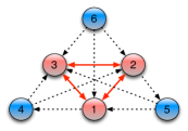
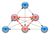
The reconstructed networks are represented in Fig. 3. There are three measured (red) nodes, labeled $1,2,3$ and by the analysis above, there are at least three hidden nodes such that the corresponding realization is consistent with the dynamical structure function. The red connections between measured nodes are the same for all candidate networks which is in accordance with Proposition 1. Dashed lines correspond to the connections between hidden and measured nodes.

Figure 3: Topologies corresponding to the four $[{Q},{P}]$ minimal realizations. The measured nodes are colored red, while the hidden ones blue. Red connections between measured nodes are the same for all the networks due to Proposition 1. Each node has a self-loop but we omit it for simplicity.

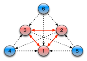
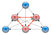
From a biological perspective, this indicates that there are at least $3$ unmeasured species interacting with the measured species. Of course, the “true” biological system might be even more complicated, i.e., it might have more than $6$ species. Yet, when more states are measured, the dynamical structure functions can be easily updated and a new search for a minimal realization of the updated system can be performed to reveal the corresponding minimal number of hidden states.

V Conclusions

In this paper, we have presented a method for obtaining a minimal order realization consistent with a given dynamical structure function. We show that the minimal order realization of a given dynamical structure function can be achieved by choosing a constant diagonal matrix ${R}^{*}$. This provides a way to estimate the complexity of the system by determining the minimal number of hidden states that needs to be considered in the reconstructed network. For example, in the context of reconstruction of biological networks from data, it helps to understand the minimal number of unmeasured molecules in a particular pathway.

VI Acknowledgement

The authors want to thank the anonymous reviewers for their feedback which has helped in improving the quality of the manuscript. Guy-Bart Stan, Ye Yuan and Jorge Gonçalves gratefully acknowledge the support of EPSRC under the projects EP/E02761X/1, EP/I03210X/1 and the support of Microsoft Research through the PhD Scholarship Program of Ye Yuan. Sean Warnick gratefully acknowledges the support of grants AFRL FA8750-09-2-0219 and FA8750-11-1-0236. Guy-Bart Stan also gratefully acknowledges the support of the EPSRC Centre for Synthetic Biology and Innovation at Imperial College, London.

Proof of the claim in Step $2$ of the proposed algorithm:

Proof:

Using results from Section $4$ of [12], if a pole of $[s{Q}~{}~{}s{P}]$, say $\lambda_{i}$, is cancelled by ${N}=(s{I}-{R}^{*})s^{-1}\triangleq{C}_{2}({A}_{2}-sI)^{-1}{B}_{2}+{I}$, then the realization of the cascade $(s{I}-{R})s^{-1}[s{Q}~{}~{}s{P}]$ loses observability. In this case, it follows that there exists a nonzero vector ${w}_{i}=[{w}_{1,i}^{T},{w}_{2,i}^{T}]^{T}$ such that

$$\begin{bmatrix}{A}_{1}-\lambda_{i}{I}&{0}\\ {B}_{2}{C}_{1}&{A}_{2}-\lambda_{i}{I}\\ {C}_{1}&{C}_{2}\end{bmatrix}\begin{bmatrix}{w}_{1,i}\\ {w}_{2,i}\end{bmatrix}={0}.$$

The first equation shows that ${w}_{1,i}$ is an eigenvector of ${A}_{1}$ corresponding to $\lambda_{i}$. Since ${A}_{1}$ is diagonal, ${w}^{T}_{1,i}=\begin{bmatrix}0&\ldots&0&1_{i^{th}}&0&\ldots&0\end{bmatrix}\in\mathbb{R}^{1\times l}$. Therefore, we have

$$\begin{bmatrix}{A}_{2}-\lambda_{i}{I}&{B}_{2}\\ {C}_{2}&{I}\end{bmatrix}\begin{bmatrix}{w}_{2,i}\\ {C}_{1}{w}_{1,i}\end{bmatrix}={0}.$$

Noticing that ${C}_{1}{w}_{1,i}={E}_{i}$ and that

$$\begin{bmatrix}{I}&{0}\\ -{C}_{2}({A}_{2}-s{I})^{-1}&{I}\end{bmatrix}\begin{bmatrix}{A}_{2}-s{I}&{B}_{2}\\ {C}_{2}&{I}\end{bmatrix}=\begin{bmatrix}{A}_{2}-s{I}&{B}_{2}\\ {0}&{N(s)}\end{bmatrix},$$

we obtain, since $\lambda_{i}\neq 0$ is not a pole of $N$,

$${N}(\lambda_{i}){E}_{i}={0}.$$ (13)

In summary, designing ${R}^{*}$ to cancel any pole $\lambda_{i}$ of $[s{Q}~{}~{}s{P}]$ is equivalent to imposing that eq. (13) holds. The next question is: given $[s{Q}~{}~{}s{P}]$ what is the maximal number of poles that can be cancelled by ${N}$, i.e., what is the largest number of poles for which eq. (13) is satisfied?

To answer this, notice that ${E}_{i}[j]$ being nonzero for some $j$, implies that there exists at least one nonzero element in the $j^{th}$ row of ${E}_{i}$. In this case, satisfying eq. (13) imposes that the $j^{th}$ diagonal element of ${N}(\lambda_{i})$ is $0$, i.e., the $j^{th}$ diagonal element of ${R}^{*}$ is $\lambda_{i}$. In other words, a nonzero element in ${E}_{i}$ corresponds to a fixed value in the corresponding diagonal position in ${R}^{*}$. Since ${R}^{*}$ is a constant diagonal matrix then any pair of orthogonal vectors in $\{{E}_{1},\cdots,{E}_{l}\}$ does not intervene in the choice of an element on the diagonal of ${R}^{*}$. ∎

Algorithm to find $\phi$ and $\Phi$:
As is presented in [16], an undirected graph is denoted by $\mathcal{G}=(\mathcal{V},\mathcal{E})$ where $\mathcal{V}=\left\{\nu_{1},\ldots,\nu_{l}\right\}$ is the set of nodes and $\mathcal{E}\subset\mathcal{V}\times\mathcal{V}$ is the set of edges.

For our purposes, we construct an undirected graph $\mathcal{G}_{a}$ using the following rules:

• A node is associated with each vector in the set $\{{E}_{1},\cdots,{E}_{l}\}$. There are thus $l$ nodes in the considered graph.

• An undirected edge $(i,j)$ is drawn between node $i$ and node $j$ if the equality ${E}_{i}^{T}{E}_{j}=0$ is satisfied.

It is easy to see that the maximum cardinality of the set $\Phi$ corresponds to the maximum number of nodes in a complete subgraph $K_{n}$ of the graph $\mathcal{G}_{a}$.

Although the problem of finding a largest complete subgraph in an undirected graph is a NP-hard problem, methods to this end have been well-studied in [17]. To our best knowledge, for an arbitrary graph, the fastest algorithm has a complexity of $\mathcal{O}(2^{n/4})$[18]. Therefore, we can use these methods to obtain a largest complete subgraph and consequently compute the corresponding set $\Phi$ and its corresponding cardinality $\phi$.

References

- [1] L. Ljung. System Identification–Theory for the User. Prentice Hall, 1999.
- [2] E. Yeung, J. Goncalves, H. Sandberg, and S. Warnick. “The Meaning of Structure in Interconnected Dynamic Systems,” invited contribution to IEEE Control Systems Magazine, Special Issue on Designing Controls for Modern Infrastructure Networks, Organizer: S. Roy, 2009. Working paper available at http://arxiv.org/pdf/1108.2755v1.pdf.
- [3] K. Zhou, J. Doyle and K. Glover, Robust and Optimal Control. Prentice Hall, 1996.
- [4] J. Gonçalves and S. Warnick, “Necessary and Sufficient Conditions for Dynamical Structure Reconstruction of LTI Networks”, IEEE Transactions on Automatic Control, 53(7): 1670-1674, 2008.
- [5] R. Howes, L. Eccleston, J. Gonçalves, G.B. Stan, and S. Warnick, “Dynamical Structure Analysis of Sparsity and Minimality Heuristics for Reconstruction of Biochemical Networks,” Proceedings of the 47th IEEE Conference on Decision and Control (CDC 2008), Cancun, Mexico, 9-11 December, 2008.
- [6] R. Howes, Application and Properties of Dynamical Structure Functions. Undergraduate Honors Thesis, Brigham Young University, Provo, UT, 2008.
- [7] J. Gonçalves and S. Warnick, “Systems-Theoretic Approaches to Network Reconstruction,” Control Theory and Systems Biology, Eds. B. Ingalls and P. Iglesias, MIT Press, 2009, pp. 265-296.
- [8] E. Yeung, J. Gonçalves, H. Sandberg, and S. Warnick, “Representing Structure in Linear Interconnected Dynamical Systems,” Proceedings of the 49th IEEE Conference on Decision and Control (CDC 2010), Atlanta, Georgia, USA, 15-17 December, 2010.
- [9] E. Yeung, Network Modeling in LTI Dynamical Systems : Reconstruction, Reduction, and Representation, Undergraduate Honors Thesis, Brigham Young University, Provo, UT, 2010.
- [10] E. Yeung, J. Gonçalves, H. Sandberg and S. Warnick, “Mathematical Relationships Between Representations of Structure in Linear Interconnected Dynamical Systems,” Proceedings of the American Control Conference (ACC 2011), San Francisco, CA, USA, 29 June - 1 July, 2011.
- [11] Y. Yuan, G. Stan, S. Warnick and J. Gonçavles, “Robust Dynamical Network Reconstruction from Data,” Special Issue on System Biology, Automatica, 47(6): 1230-1235, 2011.
- [12] S. Skogestad and I. Postlethwaite, Multivariable Feedback Control-Analysis and Design. Wiley,1996.
- [13] E. G. Gilbert, “Controllability and Observability in Multivariable Control Systems,” J.S.I.A.M. Control Ser. A, 1: 128-151, 1963.
- [14] Y. Yuan, Decentralised Network Prediction and Reconstruction Algorithms. Ph.D. Thesis, Cambridge University, 2012. Available online http://www-control.eng.cam.ac.uk/~yy311/thesis.pdf.
- [15] F. Fallside, Control System Design by Pole-Zero Assignment. Academic Press INC. LTD.
- [16] C. Godsil and G. Royal, Algebraic Graph Theory. New York: Springer-Verlag, 2001.
- [17] I. Bomze, M. Budinich, P. Pardalos, M. Pelillo, “The Maximum Clique Problem”, Handbook of Combinatorial Optimization, 1999.
- [18] J. Robson, “Finding a Maximum Independent Set,” J. Algorithm, 7:425-440, 1986.
Proof of the claim in Step of the proposed algorithm:
Proof:
Using results from Section of [12], if a pole of , say , is cancelled by , then the realization of the cascade loses observability. In this case, it follows that there exists a nonzero vector such that
The first equation shows that is an eigenvector of corresponding to . Since is diagonal, . Therefore, we have
Noticing that and that
we obtain, since is not a pole of ,