Detailed Abundances of Two Very Metal-Poor Stars in Dwarf Galaxies

Abstract

The most metal-poor stars in dwarf spheroidal galaxies (dSphs) can show the nucleosynthetic patterns of one or a few supernovae. These supernovae could have zero metallicity, making metal-poor dSph stars the closest surviving links to Population III stars. Metal-poor dSph stars also help to reveal the formation mechanism of the Milky Way halo. We present the detailed abundances from Keck/HIRES spectroscopy for two very metal-poor stars in two Milky Way dSphs. One star, in the Sculptor dSph, has [Fe I$\rm{/H]}=-2.40$. The other star, in the Ursa Minor dSph, has [Fe I$\rm{/H]}=-3.16$. Both stars fall in the previously discovered low-metallicity, high-[$\alpha$/Fe] plateau. Most abundance ratios of very metal-poor stars in these two dSphs are largely consistent with very metal-poor halo stars. However, the abundances of Na and some $r$-process elements lie at the lower end of the envelope defined by inner halo stars of similar metallicity. We propose that the metallicity dependence of supernova yields is the cause. The earliest supernovae in low-mass dSphs have less gas to pollute than the earliest supernovae in massive halo progenitors. As a result, dSph stars at $-3<{\rm[Fe/H]}<-2$ sample supernovae with ${\rm[Fe/H]}\ll-3$, whereas halo stars in the same metallicity range sample supernovae with ${\rm[Fe/H]}\sim-3$. Consequently, enhancements in [Na/Fe] and [$r$/Fe] were deferred to higher metallicity in dSphs than in the progenitors of the inner halo.

1. Introduction

The theory of the hierarchical assembly of the Milky Way (MW) from smaller structures (Searle & Zinn, 1978; White & Rees, 1978) has enjoyed wide observational support in the past two decades. The ongoing disruption of the Sagittarius dwarf galaxy (Ibata et al., 1994) provided dramatic evidence for presently active hierarchical merging. Odenkirchen et al. (2001) discovered tidal tails around the globular cluster Palomar 5, indicating that both galaxies and clusters participate in the stellar conglomeration. Perhaps most strikingly, the Sloan Digital Sky Survey has permitted the discovery of numerous tidal streams (Belokurov et al., 2006) along many different lines of sight. The ubiquity of these merger events makes it clear that the MW halo is still being formed and that its constituents are many small objects composed of both stars and dark matter.

Much of the study of the merging process concerns the precise nature of the building blocks. One test of the nature of the halo is its chemical similarity to smaller objects. The advent of 8–10 m telescopes permitted the first detailed chemical analyses of stars in MW dwarf spheroidal galaxies (dSphs). Shetrone et al. (2001, 2003) discovered that the detailed abundance patterns of stars in dSphs did not agree with stars of similar metallicity in the inner halo. Therefore, the surviving dSphs cannot be identical to the primary constituents of the inner halo.

Robertson et al. (2005) and Font et al. (2006a, b) proposed a solution to the chemical discrepancy. The inner halo was not built from galaxies like the surviving dSphs. Instead, it was built from galaxies closer in stellar mass and gas content to dwarf irregular galaxies. Cosmological simulations showed that the inner halo was built very early by massive satellite galaxies. In contrast, the surviving dSphs are small galaxies that formed stars inefficiently. Also, they have had over 10 Gyr to alter their stellar populations, including their chemical compositions. The surviving dSphs and their siblings are currently participating in the construction of the outer halo, which spans a much longer duration than the rapid assembly of the inner halo.

In the past few years, several studies have attempted to discern whether galaxies like the surviving dSphs can contribute the most metal-poor stars to the MW halo. The search for chemical consistency was driven by the desire to find a source for the most metal-poor stars in the halo. Helmi et al. (2006) claimed that the dSphs are free of stars with ${\rm[Fe/H]}<-3$ based on line strengths of the infrared Ca II triplet. However, Kirby et al. (2008) discovered such stars in the MW’s ultra-faint dwarf galaxies (Simon & Geha, 2007). Several studies (e.g., Frebel et al., 2010a, b; Simon et al., 2010; Norris et al., 2010) established the similarity between these stars’ abundances and those of the halo. A subsequent, corrected analysis of the Ca II triplet metallicity distributions of classical dSphs has uncovered extremely metal-poor stars (Starkenburg et al., 2010), and new extremely metal-poor stars have now been discovered in the classical dSphs using other spectroscopic methods (Kirby et al., 2009, 2010; Cohen & Huang, 2009, 2010; Frebel et al., 2010a; Tafelmeyer et al., 2010).

Despite the general agreement, some discrepant abundance patterns persist between the dSphs and the halo. For example, [Na/Fe] tends to be lower in the dSphs than in the halo (Cohen & Huang, 2010), and the neutron-capture elements are much more enhanced in dSph stars than in halo stars at ${\rm[Fe/H]}=-1$ (Letarte et al., 2010). As a result of these minor discrepancies, it is interesting to study chemically peculiar dSph stars. Kirby et al. (2010, K10) measured the abundances of thousands of red giants in eight MW dSphs from medium-resolution spectroscopy. Some of these are both very metal-poor and bright enough for high-resolution spectroscopic follow-up. We selected two of the most interesting stars in this sample. One of the stars is in the Sculptor dSph, and, according to K10, it is magnesium-enhanced ($\rm{[Mg/Fe]}=+0.69\pm 0.16$). The other is in the Ursa Minor dSph, and it is extremely metal-poor (${\rm[Fe/H]}=-3.62\pm 0.35$). In order to verify these interesting abundances and to measure the abundances of many elements not accessible to K10’s study, we obtained Keck/HIRES (Vogt et al., 1994) spectra of both stars. The details of some of our measurement and analysis methods are somewhat new. Therefore, we spend much of this article describing our procedures.

In Section 2, we describe our HIRES observations and data reduction. In Section 3 we describe our technique for measuring absorption line strengths and their uncertainties. Section 4 details our method for estimating abundances and uncertainties from the line strengths. We interpret our measurements in Section 5 and summarize our work in Section 6.

2. Observations and Data Reduction

2.1. Target Selection

Targets were selected from K10’s catalog of medium-resolution spectroscopic abundance measurements. This catalog contains Fe, Mg, Si, Ca, and Ti abundance measurements from spectral synthesis of Keck/DEIMOS (Faber et al., 2003) observations. The sample of 2961 stars is unbiased with respect to metallicity, and it reaches far down the red giant branch ($V\approx 22$) in eight MW dSphs. However, the limited spectral range and resolution of DEIMOS restricts the precision of the abundance measurements and the number of elements that can be measured. Therefore, we selected one metal-poor star in each of two dSphs from the catalog for high-resolution spectroscopic follow-up to reveal whether the abundance pattern of this star is consistent with similarly metal-poor stars in the MW halo and other dSphs.

2.2. Observations

Table 1 gives coordinates, photometry, and observational details for all of our targets. In addition to Scl 1019417 and UMi 20103, we included in our study two metal-poor abundance standards previously observed with HIRES by J. Cohen: HD 115444 and HD 122563. Because our equivalent width measurement technique differed from Cohen’s previous work (e.g., Cohen et al., 2003), we re-analyzed these spectra to demonstrate the validity of our abundance measurements. The $V$ magnitude for HD 115444 was taken from the TASS Mark IV survey (Droege et al., 2006; Richmond, 2007), and the $J$ and $K$ magnitudes were taken from 2MASS (Skrutskie et al., 2006). All of the photometry for HD 122563 was taken from Ducati (2002).

We configured HIRES optimally for faint, metal-poor red giants. For the program star observations, we used the red cross-disperser with a spectral range of 3927–8362 Å. The slit width was 1.15”, and the slit length was 7”, the maximum length that disallows overlap of the bluest orders. The spectral resolution depends primarily on the slit width. When the seeing is smaller than the slit width, and the guiding is good, the spectral resolution is smaller than that corresponding to the projected width of the slit. Therefore, the spectral resolution was better for UMi 20103 than for Scl 1019417, which suffered from the poor seeing at an airmass of $\sim 2$.

The spectrograph was configured differently for the abundance standards than for the program stars because the abundance standards were observed under programs with different science goals. The slit width for HD 115444 was only 0.4”. The ultraviolet cross-disperser was used for HD 122563. The reddest wavelength for this spectrum is just 5993 Å, but our line list includes few lines beyond that wavelength.

The spatial axis of the HIRES CCDs is oversampled, with a plate scale of 0.12” per pixel. Therefore, we binned the detector readout by two pixels in the spatial axis. We did not bin the dispersion axis. The dispersion is about 0.020 Å per pixel at 5138 Å.

The next section describes the use of DAOSPEC to measure equivalent widths. Two products of DAOSPEC are the FWHMs of absorption lines and the residual spectrum, after all absorption lines have been subtracted. We measured the spectral resolving power by calculating the median of the wavelengths of all lines measured with DAOSPEC divided by their FWHMs. We measured the SNR of each spectrum by calculating the standard deviation of pixels between 5700 Å and 5800 Å in the residual spectrum. The SNR per pixel is the inverse of this quantity. To convert to SNR per resolution element, we multiplied by the square root of the number of pixels occupied by the FWHM of weak absorption lines near 5750 Å. Table 1 lists spectral range, resolving power, and SNR.

The resolution of spectral features is limited by the stellar macroturbulence. Gray (2008) showed that red giants typically have a macroturbulence of $\sim 5$ km s^-1, corresponding to a maximum resolving power of $R\sim 60\,000$. Therefore, the narrower slit used for HD 115444 does not ensure that stellar features will appear at the instrumental resolution, $R=86\,600$. Indeed, the measured resolving power for this star is $37\,300$. Taking into account the spectrograph’s line spread function, we estimate that the macroturbulence for this star is 7 km s^-1, consistent with Gray’s (2008) relations.

In addition to science exposures, we also obtained exposures of a thorium-argon arc lamp, a quartz flat lamp, and bright stars to trace the echelle orders along the detector.

2.3. Data Reduction

We reduced the raw frames into one-dimensional spectra using the HIRES data reduction software MAKEE. With no user input, this pipeline subtracts the bias level, flat fields the images, extracts a single one-dimensional spectrum for each echelle order along the traces determined from the trace star, and finds the wavelength solution—including the heliocentric correction—from the arc lamp exposure. We modified MAKEE slightly to interpolate over bad columns in the second-generation HIRES CCD mosaic, installed in 2004. Some spectral regions were observed on two or three blue echelle orders. There were gaps of up to 46 Å between the reddest echelle orders.

We ran MAKEE on each exposure individually. For the final spectrum, we added together all of the one-dimensional spectra for a single object. MAKEE also provides a $1\sigma$ error spectrum for each exposure. We constructed a final error spectrum by adding together the individual error spectra in quadrature. MAKEE determined the wavelength solution from a sixth-order polynomial fit. DAOSPEC (Section 3) required a linear wavelength scale. Therefore, we linearly rebinned the spectrum for each order.

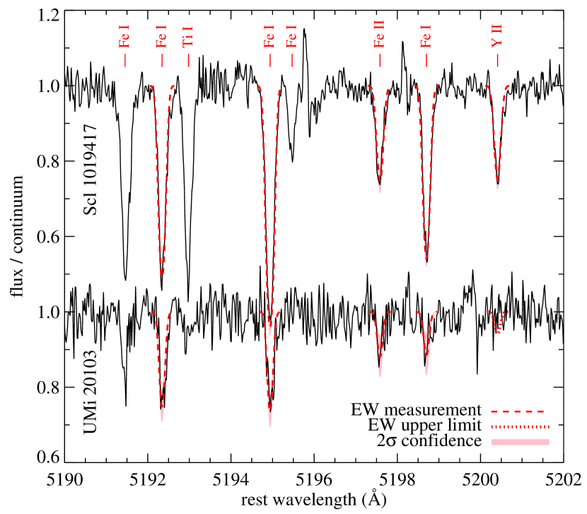
Figure 1.— A small region of the HIRES spectra of Scl 1019417 and UMi 20103. Prominent absorption lines are labeled with the responsible element and ionization state. Lines used for abundance measurements were fitted with saturated Gaussians (dashed red lines). The light, red shaded regions illustrated the $2\sigma$ confidence intervals on the EWs based on line fits to different Monte Carlo realizations of the spectra. The $2\sigma$ upper limit on the EW for Y II $\lambda 5200$ in UMi 20103 is shown as a dotted red line.

Figure 1 shows a small region (5190–5202 Å) of the HIRES spectra for the two program stars. A comparison between the two spectra shows the lower SNR of UMi 20103. It is also clear that UMi 20103 has weaker metal absorption lines than Scl 1019417. The weaker lines are due mostly to the higher effective temperature and partly to the lower metallicity of UMi 20103.

3. Measurement of Equivalent Widths

3.1. DAOSPEC

We measured equivalent widths (EWs) in each spectrum using DAOSPEC (Stetson & Pancino, 2008). This program automatically determines the continuum shape, absorption line centers, and line strengths. First, DAOSPEC iteratively fits and subtracts saturated Gaussian profiles (as discussed by Stetson & Pancino, 2008) from the observed spectrum. Then, it fits a polynomial to the residual flux. We chose a polynomial order of 20. The program detects additional lines in successive iterations, and it terminates when the residual spectrum is consistent with flat noise. This procedure is particularly adept at measuring the EW of each component of partially blended lines. The data products are the continuum shape, residual spectrum, radial velocity, and a line list, including central wavelengths, line widths, and line strengths.

Each echelle order has its own instrumental response function and consequently its own continuum shape. Therefore, we ran DAOSPEC on each echelle order independently. We forced the resolving power ($\lambda/\Delta\lambda$) to be constant with wavelength, as is appropriate for echelle spectrographs.

DAOSPEC cross-correlates the list of detected lines with the user’s list. Our line list was identical to that of the Keck Pilot Project (Carretta et al., 2002; Cohen et al., 2003). We determined the radial velocity for each star by examining the difference between the measured line centers and the predicted line centers from the line list. Each line gave an independent measurement of the radial velocity. In Table 1, we quote the mean and the error on the mean of all of the radial velocity measurements for each star.

Although DAOSPEC reported the EW for almost every line in the line list, some lines required manual intervention. We built a graphical user interface, called hiresspec, in IDL to display HIRES spectra and measure EWs. Hiresspec shows the linearized spectra of all echelle orders divided by the continuum polynomial previously determined by DAOSPEC. Each line from the line list is marked with the responsible elemental species. If DAOSPEC successfully measured the line’s EW and FWHM, then hiresspec shows the corresponding saturated Gaussian profile. If DAOSPEC failed to measure a line’s EW, which happened rarely, then the user may request that hiresspec fit a saturated Gaussian to the line. The FWHM of the line is fixed based on the spectrum’s constant resolving power ($\lambda/\Delta\lambda$). Hiresspec uses the Levenberg-Marquardt minimization code MPFIT (Markwardt, 2009) to determine the EW. If a line is not detected above the noise, the user may request hiresspec to estimate an upper limit. To do this, hiresspec uses MPFIT to find the EW of saturated Gaussian that is too strong for the observed spectrum at the $2\sigma$ confidence interval.

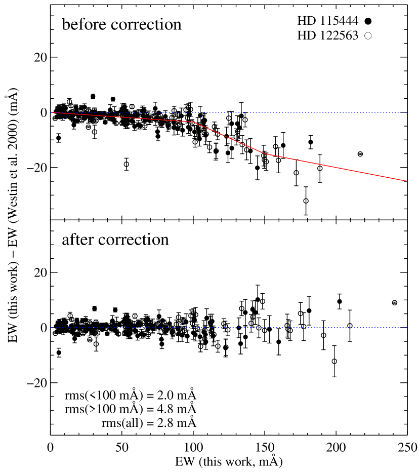
Figure 2.— Comparison of the EWs measured here with those of Westin et al. (2000) for the two abundance standards HD 115444 and HD 122563. The error bars are calculated from our measurements only. They are the larger of $\delta$EW_noise or $\delta$EW_DAO. The top and bottom panels show the EWs before and after an empirical correction for the imperfect line profile. The red line in the top panel shows the magnitude of the correction as a function of EW. In the bottom panel, the rms is given for three groups: lines that Westin et al. measured to be less than and greater than 100 mÅ and all lines.

Figure 2 compares our EW measurements with those of Westin et al. (2000), who also observed HD 115444 and HD 122563. Our EWs are about 3.5% weaker than those of Westin et al. at $\rm{EW}<100$ mÅ and about 10% weaker at $\rm{EW}>150$ mÅ. Westin et al. fit Gaussians whereas we fit saturated Gaussians. The widths of their Gaussians were determined separately for each line whereas DAOSPEC fixes $\Delta\lambda/\lambda$. Westin et al. determined the continuum manually for each line whereas we determined a global continuum for each echelle order. These are the primary causes for discrepancy between the two sets of EW measurements.

Our saturated Gaussian fits are not perfect representations for the HIRES line spread profile. The profile is complex due to the nature of the instrument and, for longer exposures, changes in seeing during the night. We compared the EWs computed from saturated Gaussians to EWs computed from direct summation for lines at a variety of strengths in both HD 115444 and HD 122563. We found that direct-sum EWs were in general closer to Westin et al.’s EWs than our saturated Gaussian EWs. This result suggests that our saturated Gaussian fits underestimate the true EWs.

Our error estimates (Section 3.2) required an automated method of determining the spectral continuum and measuring EWs. Therefore, we chose to use DAOSPEC despite the underestimated EWs. Instead, we applied an empirical correction to the EWs, depicted in the top panel of Figure 2. For each line with $\rm{EW}<100$ mÅ, we raised the EW by 3.5%. For each line with $\rm{EW}>150$ mÅ, we raised the EW by 10%. The correction factor for lines with $100~{}{\rm m\AA}<{\rm EW}<150~{}{\rm m\AA}$ was $(0.13({\rm EW/m\AA})-9.5)\%$.

Table 2 lists the EW measurements used in the abundance analysis. Figure 1 shows EW measurements for some metal absorption lines in the two program stars. All of these measurements were made with DAOSPEC.

Some strong lines are not used in the abundance measurements. We eliminated Fe and Ti lines with $\log(\rm{EW}/\lambda)\gtrsim-4.6$ from the line list. These lines are roughly on the saturated portion of the curve of growth. They are weakly sensitive to abundance and mostly serve to add noise to the abundance measurements of Fe and Ti, which have plenty of weaker lines. Only lines used in the abundance analysis appear in Table 2. The upper limits shown in Table 2 are only for those species (element and ionization state) that do not have a secure measurement of any absorption line. They are marked with a less-than symbol ($<$). Table 2 includes only the most restrictive line–the line that yields the lowest abundance–of any species with an upper limit on its abundance.

3.2. Error Estimates

The HIRES spectra of UMi 20103 and Scl 1019417 have moderately low SNR. The standard technique of calculating abundance errors, from the variance of the abundances determined from lines of the same species, may be inadequate for these spectra. As a result, we devised a method for estimating the errors in EWs and abundances caused by spectral noise.

MAKEE produces an error spectrum, which is mostly random Poisson noise. The high spectral resolution makes systematic errors, such as imprecise subtraction of night sky lines, negligible. As a result, the error spectrum may be used to create a different noise realization of the observed spectrum. The resampled spectrum ($F_{r}(\lambda)$) is equal to the original spectrum with the addition of Gaussian random noise proportional to the error at each pixel ($\sigma(\lambda)$):

$$F_{r}(\lambda)=F(\lambda)+R\sigma(\lambda)$$ (1)

where $R$ is a different random number for each pixel, drawn from a unit normal distribution ($e^{-x^{2}/2}$).

We resampled each of the four HIRES spectra 100 times. We ran each different noise realization through DAOSPEC. DAOSPEC treated each noise realization independently, with no information from the original spectrum. We then used hiresspec in an automated mode to measure EWs for any lines listed in Table 2 that DAOSPEC missed. Finally, we applied the empirical correction to EWs described in the previous section. The final list of EW measurements for each noise realization contained just as many absorption lines as the original spectrum. The final products of the EW measurement process were 101 line lists for each of the four HIRES spectra with EW measurements: EW measurements for the original spectrum and 100 EW measurements from noise-added spectra for the same absorption lines.

The EWs quoted in Table 2 are the EWs measured from the original spectrum. The random errors, $\delta$EW_noise, are the standard deviations among the EW measurements from noise-added spectra. It may seem that adding noise to the spectrum would inflate the error estimate. In other words, the original spectrum already has noise $\sigma(\lambda)$. Therefore, a noise-added spectrum has noise $\sqrt{2}\sigma(\lambda)$. However, half of the noise in every noise-added spectrum is from the same noise realization. That component does not change from spectrum to spectrum. Therefore, the scatter in EWs among the 100 noise realizations comes only from the additional component of $\sigma(\lambda)$, not from the unchanging original noise.

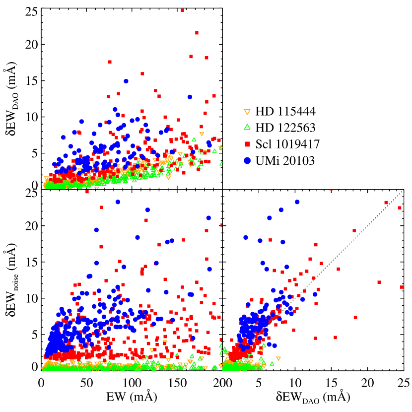
Figure 3.— EWs and errors for the four stars observed with HIRES. Errors are presented both as random measurement uncertainty ($\delta$EW_noise) and the systematic error determined by DAOSPEC ($\delta$EW_DAO). The dotted line in the lower right panel is one-to-one.

DAOSPEC also reports errors on EWs, which we call $\delta$EW_DAO. This error estimate is more inclusive than $\delta$EW_noise. It includes uncertainty on the EW not only due to spectral noise but also due to systematic errors caused by blended lines and imprecise continuum placement. Figure 3 shows how $\delta$EW_noise and $\delta$EW_DAO depend on EW and how the errors relate to each other. For the high-SNR spectra of HD 115444 and HD 122563, $\delta$EW_DAO generally exceeds $\delta$EW_noise, especially for strong lines. In these cases, systematic error dominates the spectral Poisson noise. The spectra of Scl 1019417 and UMi 20103 have lower SNRs. As a result, spectral Poisson noise dominates the EW errors, and $\delta$EW_noise and $\delta$EW_DAO agree well with each other.

4. Measurement of Atmospheric Parameters and Abundances

We computed abundances using ATLAS9 (Kurucz, 1993) model atmospheres and the code MOOG (Sneden, 1973) with an improved treatment of scattering (Sobeck et al., 2011). This section describes how we determined the atmospheric parameters (effective temperature, surface gravity, microturbulent velocity, metallicity, and alpha enhancement) and how we subsequently computed abundances from EWs and their errors.

4.1. Atomic Data

We used the atomic line list of the Keck Pilot Project (Carretta et al., 2002). Cohen et al. (2003) described the list in detail. Where available, we updated the list with version 4.1.1 of the National Institute of Standards and Technology (NIST) Atomic Spectra Database (Ralchenko et al., 2011). We also treated hyperfine structure (see Section 4.9) with Cohen et al.’s (2004) compilation of hyperfine transitions. (For simplicity, Table 2 lists only one line for each hyperfine complex.) Where available, we used damping constants from Barklem et al. (2000) and Barklem & Aspelund-Johansson (2005). Otherwise, we used the damping constants from the Keck Pilot Project’s line list.

4.2. Determination of Atmospheric Parameters

The most important atmospheric parameter in the determination of abundances is the effective temperature ($T_{\rm{eff}}$). This parameter may be determined from photometry and stellar evolutionary considerations, or it may be determined directly from the spectrum with no other input. Ivans et al. (2001) described in detail the methods and advantages to calculating $T_{\rm{eff}}$ and surface gravity ($\log g$) from both the photometric and spectroscopic methods. We experimented with calculating $T_{\rm{eff}}$ from both methods.

Table 3Model Atmosphere Parameters

	Spectroscopic $T_{\rm{eff}}$					Photometric $T_{\rm{eff}}$
Parameter	HD 115444	HD 122563	Scl 1019417	UMi 20103		HD 115444	HD 122563	Scl 1019417	UMi 20103
$T_{\rm eff}$ (K)	4750	4662	4280	4799		4771	4742	4356	4855
$\delta_{\rm noise}T_{\rm eff}$ (K)	6	6	32	72		$\cdots$	$\cdots$	$\cdots$	$\cdots$
$\log g$	1.44	1.36	0.42	1.66		1.44	1.36	0.42	1.66
$\xi$ (km s-1)	2.09	2.48	2.21	2.04		2.09	2.45	2.23	2.02
$\delta_{\rm noise}\xi$ (km s-1)	0.04	0.01	0.10	0.27		0.04	0.02	0.13	0.22
$\rm{[Fe/H]}$	$-3.11$	$-2.89$	$-2.45$	$-3.15$		$-3.10$	$-2.81$	$-2.37$	$-3.09$
$\delta_{\rm noise}{\rm[Fe/H]}$	$0.01$	$0.01$	$0.04$	$0.10$		$0.01$	$0.01$	$0.03$	$0.04$
$\rm{[\alpha/Fe]}$	$+0.57$	$+0.46$	$+0.62$	$+0.37$		$+0.57$	$+0.49$	$+0.60$	$+0.37$
$\delta_{\rm noise}{\rm[\alpha/Fe]}$	$0.01$	$0.01$	$0.05$	$0.09$		$0.01$	$0.00$	$0.05$	$0.09$

First, we estimated $T_{\rm{eff}}$ and $\log g$ from photometry alone. For the dSph stars, we corrected the $V$ and $I$ magnitudes for extinction from Schlegel et al.’s (1998) dust maps: $E(V-I)=0.029$ for Sculptor and $0.042$ for Ursa Minor. From the $I_{0}$ magnitude and $(V-I)_{0}$ color, we calculated $T_{\rm{eff}}$ and $\log g$ from 12 Gyr Yonsei-Yale isochrones (Demarque et al., 2004) with ${\rm[Fe/H]}=-2.5$ and ${\rm[\alpha/Fe]}=+0.3$. We adopted distance moduli of $(m-M)_{0}=19.67\pm 0.12$ for Sculptor (Pietrzyński et al., 2008) and $19.18\pm 0.12$ for Ursa Minor (Mighell & Burke, 1999). For the bright abundance standards, distances are unavailable. Therefore, we followed the procedure of Cohen et al. (2002) to determine atmospheric parameters. Both $T_{\rm{eff}}$ and $\log g$ were determined iteratively from a combination of color-temperature relations and Yonsei-Yale isochrones. We corrected the $V$ magnitudes for extinction (Schlegel et al., 1998), and we calculated $V-J$ and $V-K$ color temperatures (Houdashelt et al., 2000) assuming an initial guess of ${\rm[Fe/H]}=-2.8$ and $\log g=1.4$. From the average of these two temperatures, we computed $\log g$ from 12 Gyr, alpha-enhanced Yonsei-Yale isochrones. Then, we recalculated color temperatures with this estimate of $\log g$. We repeated this process until $T_{\rm{eff}}$ and $\log g$ converged. The right half of Table 3, under the heading “Photometric $T_{\rm{eff}}$,” gives the photometric values of $T_{\rm{eff}}$ and $\log g$ for all four stars.

From $\log g$, we computed an initial guess for the microturbulent velocity ($\xi$) from Equation 2 of Kirby et al. (2009). We also made an initial guess at [Fe/H] and [$\alpha$/Fe], defined as the average of the available [Mg/Fe], [Si/Fe], [Ca/Fe], and [Ti/Fe] measurements. We took these measurements from K10 for the dSph stars and from Westin et al. (2000) for the abundance standards. From the five atmospheric parameters ($T_{\rm{eff}}$, $\log g$, $\xi$, [Fe/H]  and [$\alpha$/Fe]), we interpolated an ATLAS9 model atmosphere from Kirby’s (2011) grid.

With the line list and the model atmosphere, we used MOOG to compute abundances, $\epsilon$, for each line of Mg, Si, Ca, Ti, and Fe. We then calculated [Fe/H] as the average of the abundances from all of the Fe lines, regardless of ionization state. We also calculated [Mg/Fe], [Si/Fe], and [Ca/Fe], and we averaged them to obtain [$\alpha$/Fe]. These new quantities were used to interpolate a new ATLAS9 atmosphere and compute new abundances. We then measured six quantities, $m_{i}$, from the abundances derived from Fe and Ti lines:

1. $m_{1}$: The slope of abundance with excitation potential (EP), $d(\log\epsilon)/dEP$, for Fe I lines. This parameter is most affected by $T_{\rm{eff}}$.

2. $m_{2}$: The slope of abundance with reduced width, $d(\log\epsilon)/d(\log({\rm EW}/\lambda))$, for Fe I lines. This parameter is most affect by $\xi$.

3. $m_{3}$: The difference between the average Fe I abundance and the average Fe II abundance. This parameter is most affected by $\log g$.

4. $m_{4}$, $m_{5}$, and $m_{6}$: The same three quantities for Ti lines.

The slopes were computed from least-squares linear regressions. Jackknife errors, $\delta m_{i}$, were calculated for all six quantities. In general, the errors from the Fe lines were a factor of several smaller than from the less numerous Ti lines. We calculated a goodness-of-fit, $\chi^{2}=\sum_{i=1}^{6}(m_{i}/\delta m_{i})^{2}$. The IDL Levenberg-Marquardt minimizer MPFIT (Markwardt, 2009) was employed to minimize $\chi^{2}$ in successive iterations.

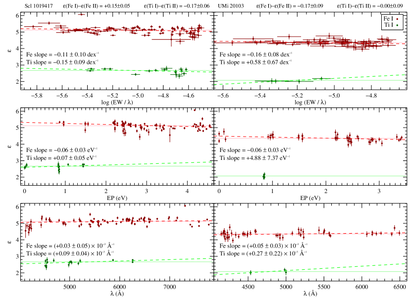
Figure 4.— Abundances in Scl 1019417 and UMi 20103 from individual lines of Fe I and Ti I as a function of the lines’ reduced width ($\rm{EW}/\lambda$, top), excitation potential (middle), and wavelength (bottom). The error bars on the abundances are the standard deviations among 100 noise realizations of the spectrum. The figure title gives the differences between the abundances of neutral and ionized species of Fe and Ti. The best combination of effective temperature and microturbulent velocity minimizes the slopes of the relations in the top two panels and the differences in elemental abundances from different ionization states of Fe and Ti. The confidence intervals on the slopes and differences between abundances of different ionization states were computed using a delete-1 jackknife.

We performed this minimization using photometric and spectroscopic temperatures. For the adopted photometric temperature, the only variable is $\xi$. It was varied until $\chi^{2}$ was minimized. For the spectroscopic temperature, both $T_{\rm{eff}}$ and $\xi$ were varied. Table 3 gives the optimized parameters for both the spectroscopic and photometric methods. In order to estimate the uncertainty introduced by spectral noise, we also computed the atmospheric parameters for all 100 noise realizations of all four spectra. The standard deviations among 100 trials for each parameter, $\delta_{\rm noise}$, are also listed in the table.

Figure 4 shows the trends of Fe I and Ti I abundances with reduced width, excitation potential, and wavelength for the spectroscopic temperatures in Scl 1019417 and UMi 20103. The lack of trends with reduced width and excitation potential show that $\xi$ and $T_{\rm{eff}}$, respectively, have been measured accurately. The lack of a trend with wavelength is merely a check that MOOG does not give different results as the continuous opacity changes from the blue to red regions of the spectrum.

Although we experimented with measuring $\log g$ from the spectrum, we found that it was degenerate with $T_{\rm{eff}}$. Particularly in the cases of HD 115444 and Scl 1019417, the $\chi^{2}$ minimum was a long, narrow valley in $T_{\rm{eff}}$–$\log g$ space that permitted a temperature range of hundreds of Kelvin. On the other hand, $\log g$ can be measured very precisely from photometry in cases where the distance is known, such as for the dSph stars. Isochrones can pinpoint $\log g$ to within 0.1. Uncertainties in the photometry and distance modulus propagate to an uncertainty in $\log g$ of only 0.05. Because Sculptor and Ursa Minor have only ancient populations (e.g., Monkiewicz et al., 1999; Carrera et al., 2002), uncertainty in the age of the star, say from 10 to 14 Gyr, contributes negligible error to $\log g$ (about 0.02). Finally, the systematic error in isochrone modeling may be quantified from the dispersion among different isochrone sets. The maximum difference between the Yonsei-Yale, Victoria-Regina (VandenBerg et al., 2006), and Padova (Girardi et al., 2002) isochrones is 0.12 for Scl 1019417 and 0.03 for UMi 20103. Therefore, we conclude that our abundance measurements are far more certain with the photometric value of $\log g$ than with a spectroscopic value. Furthermore, we assert that the small uncertainty in $\log g$ will contribute insignificantly to uncertainty in the abundance measurements. Consequently, we do not consider $\log g$ in our abundance error estimates.

As a check on the surface gravity, the top of Figure 4 gives the differences between Fe I and Fe II and between Ti I and Ti II. Ideally, these differences should be zero. However, non-local thermodynamic equilibirum (NLTE) effects can alter the photospheric ionization balance. Thévenin & Idiart (1999) identified overionization by ultraviolet radiation to be the most significant NLTE effect for Fe abundance in metal-poor stars. Essentially, the true photosphere contains fewer Fe I atoms (the minority species) for its iron abundance than the idealized LTE photosphere. The same effect applies to Ti, which has an ionization potential only 0.9 eV less than Fe. Therefore, with a photometric surface gravity, it may be impossible to find a combination of $T_{\rm{eff}}$ and $\xi$ that perfectly balances neutral and ionized species. In fact, there may be no choice of surface gravity that balances the abundances from different ionization states. The differences in Figure 4 reflect this conundrum. However, using a photometric gravity insulates our abundance measurements from the overionization effect. For consistency with most of the literature, we did not correct our Fe I abundances for overionization.

The high precision in $\log g$ afforded by photometry does not extend to $T_{\rm{eff}}$. Photometric uncertainties and systematic errors lead to temperature errors exceeding 100 K. The maximum difference between the spectroscopic and photometric temperatures among the four stars in our sample, shown in Table 3, is 80 K. The maximum difference in $\xi$ between the two methods is just 0.03 km s^-1. We consider the spectroscopic $T_{\rm{eff}}$ to be more accurate than the photometric $T_{\rm{eff}}$. For the remainder of this article, abundances are derived using the atmospheric parameters listed under “Spectroscopic $T_{\rm{eff}}$” in Table 3.

4.3. Abundance Measurements

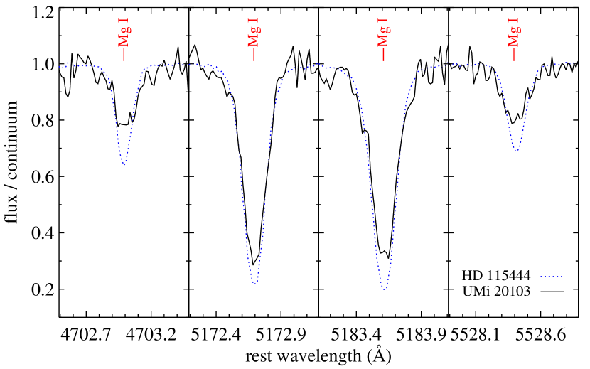
Figure 5.— Mg I lines in HD 115444 and UMi 20103. These two stars have similar atmospheric parameters. Therefore, the line strengths correspond fairly directly to the abundances. We measured $\epsilon($Mg I$)=5.00$ and $4.81$ in HD 115444 and UMi 20103, respectively.

After the optimal atmospheric parameters were determined, we interpolated the corresponding ATLAS9 model atmosphere from Kirby’s (2011) grid. The abundances used to compute opacities in the model atmosphere were not strictly consistent with the abundances of the star. We started with solar abundances (Anders & Grevesse, 1989, except that $\epsilon(\rm{Fe})=7.52$) scaled by [Fe/H]. Then we rescaled the atmospheric abundances of O, Ne, Mg, Si, S, Ar, Ca, and Ti by [$\alpha$/Fe], determined by the procedure described in Section 4.2. This model atmosphere and the line list were the inputs for MOOG. Table 4 shows the abundance results for the four stars. The table also shows the abundances relative to the solar abundances.

Figure 5 gives an example of the abundance measurements. It shows the four lines used to determine the Mg I abundance in UMi 20103. It also shows the same lines in HD 115444, which has $T_{\rm eff}$, $\log g$, and $\xi$ similar to UMi 20103. Therefore, line strengths correspond fairly directly to abundances. The Mg I lines in UMi 20103 are slightly weaker than in HD 115444, indicating that UMi 20103 has a slightly lower Mg I abundance. In fact, we measured $\epsilon($Mg I$)=5.00$ in HD 115444 and $4.81$ in UMi 20103.

We also calculated abundances using the line lists from each of the 100 Monte Carlo noise realizations of the spectrum. We estimated the abundance uncertainty due to spectral noise for each line as the standard deviation of the abundances from all 100 realizations. We call the abundance uncertainty on the $i^{\rm{th}}$ line $\delta\epsilon_{i}$. Then, we calculated the error-weighted mean abundance from all $N$ lines of a given species:

$$\epsilon=\frac{\sum_{i=1}^{N}\epsilon_{i}\delta\epsilon_{i}^{-2}}{\sum_{i=1}^{N}\delta\epsilon_{i}^{-2}}$$ (2)

Each noise realization had its own value of $\epsilon$. We estimated the uncertainty on $\epsilon$ due to spectral noise, $\delta_{\rm{noise}}\epsilon$, as the standard deviation of all 100 values of $\epsilon$.

The error estimate $\delta_{\rm{noise}}\epsilon$ does not include systematic error due to uncertainty in atomic parameters for each line. As a result, we also calculated the unbiased, weighted standard deviation among the abundances from different lines of the same species. We divided this error estimate by the square root of the number of lines, and we call it $\delta_{\rm{sys}}\epsilon$. This systematic error estimate came only from the unmodified spectrum and not from any of the noise realizations. The greater of $\delta_{\rm{noise}}\epsilon$ and $\delta_{\rm{sys}}\epsilon$ is used as the error bar in all figures.

Some elements and lines required special attention. We detail them in the following sections.

4.4. Carbon

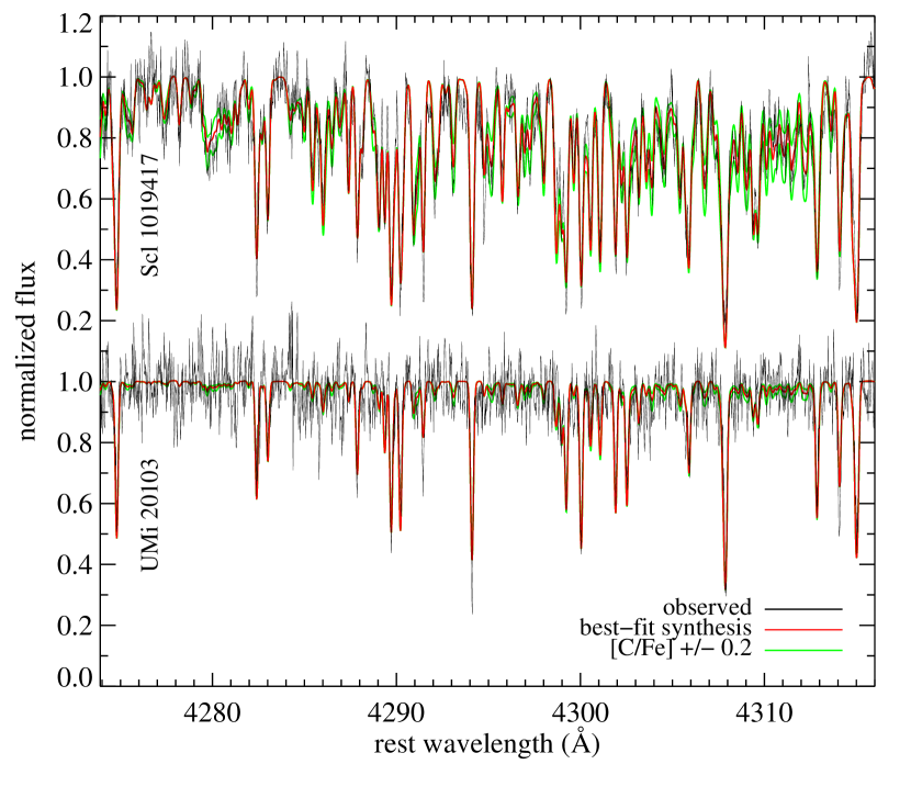
Figure 6.— The CH region of the HIRES spectra of Scl 1019417 and UMi 20103 (thin black lines). The best-fit synthetic spectra, when [C/H] was allowed to vary, are shown as thick red lines. Syntheses with [C/Fe] at 0.2 dex above and below the best-fit value are shown as green lines.

We measured the abundance of neutral carbon from spectral synthesis of the CH molecular G band. First, we used MOOG to synthesize a spectrum of the G band between 4273.9 Å and 4333.0 Å. The line list came from Jørgensen et al. (1996). We assumed that the isotopic ratio ${}^{12}\rm{C}/^{13}\rm{C}=7.0$, but our carbon abundances changed almost imperceptibly when we used different values. Then, we computed $\chi^{2}$ between the synthetic spectrum and the observed spectrum divided by the DAOSPEC continuum. The denominator of $\chi^{2}$ was the flux error estimates from MAKEE. Next, we adjusted the carbon abundance until the $\chi^{2}$ was minimized.

We refined the continuum with the residuals of the fit, an approach used for medium-resolution spectra by Shetrone et al. (2009) and K10. We fit a B-spline with breakpoints every 500 pixels (10 Å) to the quotient of the observed and best-fit synthetic spectra. Then, we divided the observed spectrum by this spline and remeasured the best-fit carbon abundance. We repeated this procedure until the best-fit carbon abundance changed by less than 0.001 dex between continuum iterations.

Figure 6 shows a region of the G band for Scl 1019417 and UMi 20103. The black lines are the observed spectra normalized by the corrected continua. The red lines are the best-fit synthetic spectra. Despite the noise in the spectrum of UMi 20103, the formal error on $\epsilon(\rm{C})$ is only 0.05 dex. However, the G band is notorious for systematic error in the line list and in $T_{\rm{eff}}$. Therefore, we assume a conservative systematic error of 0.20 dex.

4.5. Oxygen

The only oxygen line strong enough to be visible in the spectra of the stars we observed is O I $\lambda$6300.3. Unfortunately, the radial velocities of Scl 1019417 and UMi 20103 are such that separate telluric absorption lines fall exactly at 6300.3 Å in the rest frames. The strengths of the telluric lines exceed the expected strengths of the oxygen lines. As a result, attempting to remove the telluric absorption line would lead to a highly uncertain EW measurement for the oxygen lines. We estimated upper limits on oxygen abundances from O I $\lambda$6364.

4.6. Sodium

Table 5NLTE Corrections

Species	HD 115444	HD 122563	Scl 1019417	UMi20103
Na I	$-0.39$	$-0.32$	$-0.06$	$-0.20$
Al I	$+0.47$	$+0.36$	$+0.15$	$+0.55$
K I	$-0.36$	$\cdots$	$-0.41$	$-0.36$

Na I was measured as described in Section 4.3 from the Na D lines. However, we corrected the abundance for NLTE effects. Lind et al. (2011) calculated such corrections for a large range of $T_{\rm{eff}}$, $\log g$, $\xi$, and line strengths. We used the grid and interpolation routine that K. Lind kindly provided to us to calculate NLTE corrections for our own Na I measurements as well as those of Westin et al. (2000), who measured Na I from the doublet at 8190 Å. Table 5 lists NLTE abundance corrections for our stars.

The minimum surface gravity in Lind et al.’s (2011) correction table is $\log g=1.0$, larger than for Scl 1019417. However, their Figure 4 shows that the Na D NLTE correction is nearly independent of $\log g$ at 4300 K. Therefore, we used the correction for $\log g=1.0$.

4.7. Aluminum

We measured Al I from the resonance line at 3962 Å. We did not use Al I $\lambda$3944 because it is blended with CH lines. The Al resonance lines are especially subject to NLTE corrections. Andrievsky et al. (2008) computed such corrections for metal-poor stars. We consulted their Figure 2 to determine the appropriate correction for each of our stars. We linearly interpolated or extrapolated their gravity- and metallicity-dependent corrections to estimate the corrections appropriate for the atmospheric parameters of our stars. We added this correction to the Al I abundances.

4.8. Potassium

The strongest potassium line in the visible spectrum is K I $\lambda$7699. This is a strong resonance line highly subject to NLTE effects. Ivanova & Shimanskiĭ (2000) modeled the potassium atom and computed NLTE corrections to the K I abundance. We applied corrections to all of our K I abundances based on their Figure 6.

4.9. Hyperfine Splitting

Many of the elements in our repertoire (Sc II, V I, Mn I, Mn II, Co I, Cu I, Sr II, Ba II, La II, Eu II, and Pb I) are subject to hyperfine splitting of their energy levels. None of the hyperfine structure is so extended that the single-line fits are inappropriate. Therefore, these absorption lines are best treated as blends of multiple electronic transitions. Cohen et al. (2004) provided the atomic data for the components of each blend. We used the “blends” driver of MOOG to compute the abundances.

4.10. Upper Limits

For species with only upper limits on EWs, we measured abundances from all of the available upper limits. For species with more than one upper limit, the lowest abundance was used.

4.11. Comparison to Westin et al. (2000)

Figure 7.— Differences between our and Westin et al.’s (2000) abundance measurements for the two metal-poor abundance standards HD 115444 and HD 122563. All species except Fe are given as relative to the abundance of Fe measured in the same ionization state.

Figure 7 shows the differences between our measurements and those of Westin et al. (2000) for HD 115444 and HD 122563. The error bars are the quoted errors from both studies added in quadrature. We corrected Westin et al.’s Na I abundance measurement for NLTE effects as described in Section 4.6.

This comparison demonstrates that the new components of our technique (DAOSPEC, a new version of MOOG, and consistent [$\alpha$/Fe] between the model atmosphere and the measured abundances) did not cause major discrepancies with previous work. Our measurements of Fe I and Fe II are $\sim-0.15$ dex below those of Westin et al. Differences in $T_{\rm{eff}}$ between the two studies do not account for the difference because our measurements of $T_{\rm{eff}}$ are higher, which would lead to larger abundances. Instead, the difference likely comes from the different model atmosphere codes: our use of ATLAS9 “newodf” versus Westin et al.’s use of MARCS (Gustafsson et al., 1975; Edvardsson et al., 1993). We confirmed that the choice of model atmosphere code is responsible for the shift in abudances by computing abundances using the LTE version of MOOG (without an updated treatment of scattering) with Westin et al.’s line list, EWs, and atmospheric parameters. However, we used ATLAS9 model atmospheres instead of MARCS. The Fe I abundances for both stars were indeed $\sim 0.15$ dex lower than Westin et al. published.

The most discrepant species is Na I (HD 115444, $\Delta\epsilon=+0.5$). We used the strong Na D lines, whereas Westin et al. used the weaker Na I 8190 doublet. Interstellar absorption may contaminate the Na D lines, but that problem will not affect the dSph stars, which have larger absolute radial velocities.

4.12. Comparison to DEIMOS Measurements

Table 6Comparison of DEIMOS and HIRES Abundance Measurements

Spectrograph	$T_{\rm{eff}}$ (K)	$\log g$	$\xi$ (km s-1)	[Fe I/H]	[Mg I/Fe I]	[Si I/Fe I]	[Ca I/Fe I]	[Ti I/Fe I]
Scl 1019417
DEIMOS	$4175\pm 61$	$0.49\pm 0.08$	2.03	$-2.46\pm 0.11$	$+0.69\pm 0.16$	$+0.62\pm 0.18$	$+0.54\pm 0.16$	$+0.20\pm 0.13$
HIRES	$4280\pm 32$	$0.42\pm 0.08$	$2.21\pm 0.10$	$-2.40\pm 0.05$	$+0.57\pm 0.07$	$+0.53\pm 0.04$	$+0.19\pm 0.04$	$+0.08\pm 0.07$
UMi 20103
DEIMOS	$4824\pm 86$	$1.66\pm 0.05$	1.75	$-3.62\pm 0.35$	$\cdots$	$\cdots$	$+0.89\pm 0.48$	$+0.69\pm 0.84$
HIRES	$4799\pm 72$	$1.66\pm 0.05$	$2.04\pm 0.27$	$-3.16\pm 0.10$	$+0.39\pm 0.09$	$+0.38\pm 0.21$	$+0.22\pm 0.08$	$+0.25\pm 0.10$

Note. — DEIMOS measurements are taken from K10. The errors on the HIRES atmospheric parameters are the random noise error terms only (Section 4.2). The errors on the HIRES abundances are the larger of $\delta_{\rm noise}$ or $\delta_{\rm sys}$ (Section 4.3).

Table 6 shows the DEIMOS medium-resolution (K10) and HIRES high-resolution measurements for the two dSph stars. The HIRES measurements roughly agree with the DEIMOS measurements. The differences in [Fe/H] for Scl 1019417 and UMi 20103 are 0.06 dex ($0.5\sigma$) and 0.46 dex ($1.3\sigma$), respectively. Both differences are in the sense that the HIRES measurements are larger. These two stars alone do not indicate that the DEIMOS measurements tend to be too metal-poor. K10 compared DEIMOS abundances to the high-resolution literature for 132 stars. They found no systematic offset nor any trend of $\Delta{\rm[Fe/H]}$ with [Fe/H]. The differences between HIRES and DEIMOS here are consistent with random noise.

It was not possible to measure with useful precision any elements other than Fe in the DEIMOS spectrum of UMi 20103. It was possible to measure [Mg/Fe], [Si/Fe], [Ca/Fe], and [Ti/Fe] in the DEIMOS spectrum of Scl 1019417. The differences are $-0.12$ dex ($0.7\sigma$), $-0.09$ dex ($0.5\sigma$), $-0.35$ dex ($2.1\sigma$), and $-0.12$ dex ($0.8\sigma$), all in the sense that the HIRES measurements are lower. Again, it is impossible to draw conclusions from a single-star comparison. We defer to K10’s comparisons for a complete view of the accuracy of the DEIMOS measurements.

5. Discussion

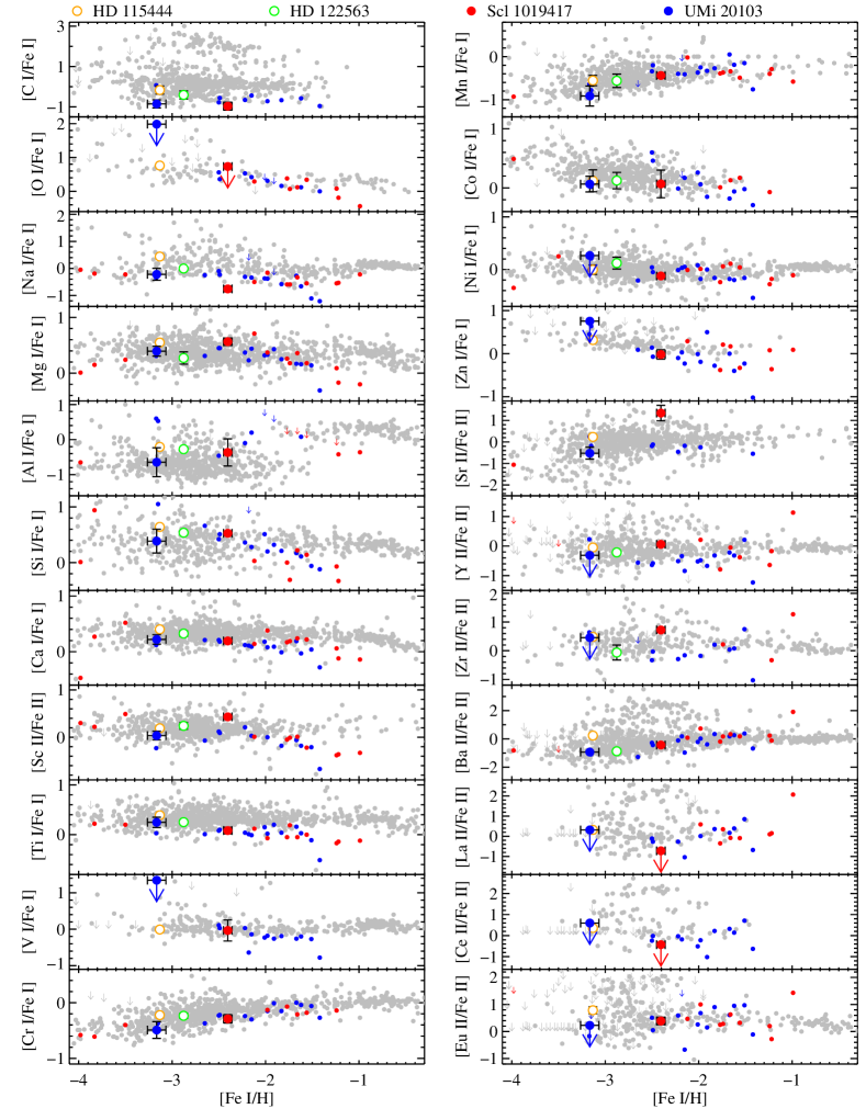
Figure 8.— Abundances in dSph stars compared to the MW halo. The program stars are shown as large, solid, colored points, and the halo abundance standards are shown as large, hollow, colored points. For comparison, other halo stars (gray points) are shown from Frebel’s (2010) compilation. Previous studies of Sculptor (Shetrone et al., 2003; Geisler et al., 2005; Frebel et al., 2010a; Tafelmeyer et al., 2010) and Ursa Minor (Shetrone et al., 2001; Sadakane et al., 2004; Cohen & Huang, 2010) are shown as small red and blue points, respectively. Error bars represent the larger of the noise or systematic error. Downward pointing arrows represent $2\sigma$ upper limits. NLTE corrections have been applied to our stars (but not necessarily the comparison sample from the literature) for Na I and Al I.

Figure 8 shows the abundances of the two program stars, Scl 1019417 and UMi 20103, along with the halo abundance standards, HD 115444 and HD 122563. For context, the figure also shows previous literature measurements for Sculptor, Ursa Minor, and the MW halo. In this section, we offer some commentary on the particular abundances of our two program stars.

5.1. The DSphs in Context

The abundance ratios we measured are not especially peculiar for very metal-poor dSph stars. These abundance ratios have been discussed at length in the literature. Tolstoy et al. (2009) and McWilliam (2010) have written recent reviews on nucleosynthesis, in particular as it concerns local galaxies.

Examining the detailed abundance patterns at a range of metallicities affords a fuller appreciation of the chemical evolution of a dSph. To first order, a sequence in metallicity is a sequence in time. As time advances, more supernovae (SNe) explode to enrich the metallicity of the dSph’s interstellar medium. Therefore, the later-forming stars have higher metallicities. This process may be modeled quantitatively and in detail (e.g., Ikuta & Arimoto, 2002; Lanfranchi & Matteucci, 2004; Kirby et al., 2011).

We compiled high-resolution abundance measurements for Sculptor and Ursa Minor from the published literature. Where necessary, we shifted their abundances to match our solar abundance scale. These are shown in Figure 8 to provide context for our own measurements. Shetrone et al. (2003) first observed Sculptor at high-resolution. They obtained VLT/UVES spectroscopy of five red giants at $R=40\,000$ with $\rm{SNR}\sim 30$ pixel^-1. Geisler et al. (2005) later obtained UVES spectra for four additional red giants at $R=20\,000$ and $\rm{SNR}\sim 90$ pixel^-1. Frebel et al. (2010a) observed the extremely metal-poor star Scl 1020549, with Magellan-Clay/MIKE at $R=33\,000$ and $\rm{SNR}\sim 35$ pixel^-1. Tafelmeyer et al. (2010) observed two additional extremely metal-poor stars in Sculptor, including the most metal-poor star known in any dSph, with VLT/UVES at $R=40\,000$ with $\rm{SNR}\sim 35$ pixel^-1. Shetrone et al. (2001) obtained the first high-resolution spectra in Ursa Minor. They observed six red giants with Keck/HIRES at $R=34\,000$ and $\rm{SNR}\sim 30$ pixel^-1. One of these, Ursa Minor K, is a carbon star, and we do not plot it. Sadakane et al. (2004) observed three red giants with Subaru/HDS at $R=45\,000$ and $\rm{SNR}\sim 55$ pixel^-1. Two of these three stars overlapped Shetrone et al.’s (2003) sample. Given Sadakane et al.’s higher resolution and SNR, we adopted their abundances instead of Shetrone et al.’s abundances. Finally Cohen & Huang (2010) observed 10 red giants in Ursa Minor with HIRES at $R=35\,000$ and $\rm{SNR}\sim 90$ per resolution element. None of these stars overlapped with the other samples, and they are all shown in Figure 8.

As has been noted many times previously, [$\alpha$/Fe] ([O/Fe], [Mg/Fe], [Si/Fe], and [Ca/Fe]) in the dSphs declines with increasing [Fe/H] at ${\rm[Fe/H]}\gtrsim-2.5$. The decrease arises from a growing contribution of the products of Type Ia SNe compared to Type II (core collapse) SNe. The former produce iron peak elements and virtually no $\alpha$ elements, whereas the latter produce $\alpha$ elements and somewhat less iron. The timescale for Type II SNe is 3–20 Myr after star formation, and the minimum delay for Type Ia SNe is about 60 Myr (e.g., Thomson & Chary, 2011). Therefore, a galaxy begins its life with the low [Fe/H] and high [$\alpha$/Fe] imposed by Type II SNe, but gradually, Type Ia SNe depress this ratio as [Fe/H] increases due to the explosion of both types of SNe. This simplistic description assumes that the galaxy does not experience any sudden star formation bursts that can produce many Type II SNe, causing an uptick in [$\alpha$/Fe] (see Gilmore & Wyse, 1991).

If Type Ia SNe experience a non-zero delay time longer than the delay for Type II SNe, then dSphs should exhibit a plateau of high [$\alpha$/Fe] at low [Fe/H], corresponding to stars formed before the advent of Type Ia SNe. Cohen & Huang (2010) identified such a plateau in Ursa Minor. Although the sparse sampling led to different maximum values of [Fe/H] for the plateau depending on the particular $\alpha$ element, Type Ia SNe seem to have begun to affect Ursa Minor’s abundance pattern somewhere in the range $-3.0\leq{\rm[Fe/H]}\leq-2.5$. This is consistent with the conclusion of Kirby et al. (2011), who found that no dSph has a high [$\alpha$/Fe] plateau that extends to ${\rm[Fe/H]}>-2.5$, except for [Ca/Fe] in Sculptor.

The existence of an [$\alpha$/Fe] plateau in Sculptor is controversial. The [$\alpha$/Fe] ratios measured by Shetrone et al. (2003) and Geisler et al. (2005) decline monotonically with metallicity. Measurements from the Dwarf Abundances and Radial Velocities Team show a plateau in [Ca/Fe] ending at ${\rm[Fe/H]}=-1.8$ (Tolstoy et al., 2009). Kirby et al. (2009, 2011) confirmed this result with medium-resolution spectroscopy of 376 Sculptor red giants. However, Kirby et al. also measured [Mg/Fe] and [Si/Fe] and found no evidence of a plateau in those $\alpha$ elements. Tolstoy et al. (2009) also presented [Mg/Fe] measurements in Sculptor. The dispersion in [Mg/Fe] at fixed [Fe/H] increases below ${\rm[Fe/H]}=-1.8$, but evidence for a plateau in [Mg/Fe] is inconclusive. Our own measurements of Scl 1019417 show that [Mg/Fe] and [Si/Fe] are consistent with rising toward lower metallicity, whereas [Ca/Fe] remains in the previously established plateau. Therefore, the distribution of [Ca/Fe] in Sculptor seems more complex than for [Mg/Fe] or [Si/Fe].

The most metal-poor stars in Sculptor (Scl 1020549, Frebel et al. 2010a; Scl07-49 and Scl07-50, Tafelmeyer et al. 2010) do not conform to this simple picture. Their [Mg/Fe] ratios are lower than the typical [Mg/Fe] ratio at ${\rm[Fe/H]}\sim-2$, and their [Si/Fe] and [Ca/Fe] span a large range. These stars are so metal-poor (${\rm[Fe/H]}\lesssim-3.5$) that they could be the direct products of one or a few Population III SNe. If so, then their abundances would reflect the specific mass- and explosion energy-dependent yields of those particular SNe. It is only when the SNe yields are averaged over progenitor mass and explosion energies that the global [$\alpha$/Fe] interpretation as the balance of Types II and Ia SNe makes sense.

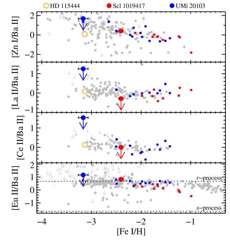
Figure 9.— Neutron-capture abundance ratios. The solar system [Eu/Ba] ratios from the $s$- and $r$-processes (Simmerer et al., 2004) are shown as dotted lines in the bottom panel. The symbols have the same meanings as in Figure 8.

The neutron-capture elements also trend with [Fe/H]. Roughly speaking, the $r$-process dominates the production of neutron-capture elements at early times (low [Fe/H]). After hundreds of Myr, thermally pulsating asymptotic giant branch (AGB) stars can expel $s$-process material. The ratio [Eu/Ba] is a diagnostic of the relative contributions of the $r$- and $s$-processes. Because Eu is produced mostly in the $r$-process, [Eu/Ba] decreases as more $s$-process sources contribute to the Ba content of the star. This phase is especially apparent in Fornax, where [Eu/Ba] decreases steeply as [Fe/H] increases (Letarte et al., 2010). The decrease of [Eu/Ba] in Sculptor continues the trend established by Fornax, but at lower [Fe/H] (Tolstoy et al., 2009). The bottom panel of Figure 9 shows the abundances of [Eu/Ba] in Sculptor, Ursa Minor, and the MW halo. The $s$-process did not contribute to MW stars by lowering [Eu/Ba] until ${\rm[Fe/H]}>-1$, but it began in Sculptor at ${\rm[Fe/H]}\sim-1.8$. Scl 1019417 is the lowest metallicity star in Sculptor with measurements of both Ba and Eu, and it shows that no $s$-process material was present in Sculptor when the dSph’s metallicity was ${\rm[Fe/H]}=-2.5$. The differences between the MW and Sculptor suggest that the MW progenitors reached a higher metallicity sooner than Sculptor. In contrast, the [Eu/Ba] in Ursa Minor does not decrease with [Fe/H]. Of course, AGB stars in Ursa Minor did produce $s$-process nuclei, just like in any other dSph. However, the star formation in Ursa Minor did not last long enough for the $s$-process material to be incorporated into stars. Alternatively, the star formation rate (SFR) was so low by the time AGB stars began to spew $s$-process nuclei that the chances of finding such a star are low.

Star formation histories derived by chemical evolution models support these interpretations. For Sculptor, the SFR began to decline 300 Myr after the first star was born in Sculptor (Kirby et al., 2011), but some star formation proceeded for up to 7 Gyr (de Boer et al., 2012). This would allow some AGB products to have polluted the more metal-rich stars in Sculptor while leaving the metal-poor stars free of the $s$-process. The star formation duration in Ursa Minor was as short as 400 Myr (Kirby et al., 2011), which would ensure that virtually no stars were contaminated by AGB ejecta.

5.2. Comparison of DSphs to the Milky Way Halo

Metal-poor stars in dSphs provide constraints on dSphs’ contribution to the MW halo. Even if the surviving dSphs are not representative of the dominant inner halo constituents (early-accreted dIrrs, Robertson et al., 2005), the most metal-poor stars would presumably have abundance patterns consistent across all types of dwarf galaxy. The earliest SNe do not have foreknowledge of the dwarf galaxy’s final stellar mass or its fate (accretion or survival). Therefore, the earliest forming, most metal-poor stars should have similar abundance patterns.

In order to compare Sculptor’s and Ursa Minor’s abundance patterns to the halo, we show Frebel’s (2010) compilation of halo star abundances as gray points in Figures 8 and 9. The abundances have been shifted to match our solar abundance scale. Note that high-resolution spectroscopy imposes a heavy bias toward bright, nearby stars. Therefore, the large majority of stars in this halo sample belong to the inner halo.

The dSph stars show the familiar discrepancy with the halo stars at ${\rm[Fe/H]}\gtrsim-2$, particularly for the $\alpha$ elements (Tolstoy et al., 2003; Venn et al., 2004). The more metal-poor dSph stars, including the two stars that comprise our sample, have abundance ratios broadly consistent with the inner halo, as previously noted by Frebel et al. (2010a, b), Simon et al. (2010), Norris et al. (2010), and Tafelmeyer et al. (2010).

However, some elements show deviation worth mentioning. First, carbon in both Scl 1019417 and UMi 20103 ($\rm{[C/Fe]}\approx-0.9$) is lower than the locus defined by halo stars. This is merely a consequence of the dSph sample, which consists exclusively of evolved red giants. Red giants dredge up carbon-depleted material as they evolve up the red giant branch (Suntzeff, 1981).

However, the dredge-up mechanism does not explain the low abundances of Na and some neutron-capture elements in both of our stars. Dredge-up does not affect Na abundances in metal-poor stars nearly as much as it affects C abundances and isotopic ratios (e.g., Spite et al., 2006). Even if dredge-up were to affect the Na abundances in metal-poor giants, it would increase [Na/Fe]. On the other hand, [Na/Fe] in metal-poor stars in dSphs is low compared to most halo stars. In fact, Scl 1019417 has one of the lowest [Na/Fe] ratios of any metal-poor star. Some neutron-capture elements in dSphs also show mild deviation from the halo. At ${\rm[Fe/H]}<-2$, [Zn/Fe], [Ba/Fe], [La/Fe], and [Ce/Fe] tend to lie along the lower edge of the envelope defined by halo stars, as shown in Figure 8. Low [Ba/Fe] ratios in extremely metal-poor stars in classical and ultra-faint dSphs have also been noted by Shetrone et al. (2001), Fulbright et al. (2004), Koch et al. (2008), Tolstoy et al. (2009), and Frebel et al. (2010b). The ratios of these neutron-capture elements to each other (Figure 9) do not appear particularly discrepant, except perhaps for the low upper limit on [La/Ba] in Scl 1019417.

We suggest that the origin for these deviations is the metallicity dependence of these elements’ SN yields. The production of Na in Type II SNe depends sensitively on the neutron excess, which depends on the initial metallicity of the exploding star (Woosley & Weaver, 1995). Lower metallicity SNe produce lower [Na/Fe] ratios. The metallicity dependence of SN yields can explain the distribution of light elements in the MW bulge (Tsujimoto et al., 2002; Lecureur et al., 2007). The metallicity dependence of the yields of neutron-capture elements is less clear. However, the $r$-process seems to consist of at least two components: the main $r$-process, which produces the full range of atomic number, and the weak $r$-process, which produces elements lighter than Ba (Ishimaru et al., 2005). (Also see Travaglio et al. 2004 and Qian & Wasserburg 2007.) Tafelmeyer et al. (2010, their Section 5.8.2) summarized the relation of the multiple components of the $r$-process to the observed abundances of extremely metal-poor stars in dwarf galaxies. Although the metallicity dependence of the yields of $r$-process elements is not well-understood, at least one potential source of the $r$-process—the lighter element primary process (Travaglio et al., 2004)—is expected to occur only in low-metallicity stars. Therefore, it is conceivable that the $r$-process yields have some metallicity dependence.

The inner halo progenitors were presumably massive galaxies (Robertson et al., 2005) that began their lives with a great deal of gas. As a result, the first SNe did not enrich the galaxy very much. Consequently, the abundance patterns seen at, say, ${\rm[Fe/H]}=-2.5$ are reflective of SNe with metallicities only slightly less than ${\rm[Fe/H]}=-2.5$. On the other hand, the surviving dSphs are small and dark matter-dominated. The gradual inflow of gas at early times (Kirby et al., 2011) ensures that the first SN will pollute a small amount of gas. As a result, a single SN can enrich the entire protogalaxy to as much as $Z=10^{-3}~{}Z_{\sun}$ (Wise et al., 2012). Therefore, the gap between a SN’s metallicity and the metallicity of the stars that formed from its ejecta is larger than in the massive inner halo progenitors. The abundance pattern of a star at ${\rm[Fe/H]}=-2.5$ in a small dSph could reflect the yields of a SN with ${\rm[Fe/H]}=-3$ or even lower. Therefore, the metallicity-dependent rise of Na and the $r$-process elements is deferred to stars with higher [Fe/H] in the dSphs than in the more massive halo progenitors.

Our suggestion is related to McWilliam et al.’s (2003) conclusion that metallicity-dependent yields caused the evolution of [Mn/Fe] in the Sagittarius dSph to differ from the MW bulge. Whereas our suggestion involves the metallicity dependence of the Type II SN yields of Na and possibly the neutron-capture elements at ${\rm[Fe/H]}<-2$, McWilliam et al.’s explanation concerns the metallicity-dependence of the Type Ia SN yield of Mn at ${\rm[Fe/H]}\sim-1$. Also, our hypothesis explains the different abundance patterns between the dSphs and the MW as a result of different masses of the star-forming gas polluted by SNe. In contrast, McWilliam et al. (2003) theorized that the difference is a result of the slower chemical evolution of Sagittarius compared to the MW bulge.

We emphasize that the abundance patterns of very metal-poor stars in dSphs do not lie outside of the boundary defined by halo stars. Rather, some abundance ratios lie on or near the boundary. Therefore, some very metal-poor stars in the high-resolution halo samples, which are heavily biased toward the inner halo, likely came from galaxies very similar to the surviving dSphs. Other very metal-poor halo stars with higher [Na/Fe] and [$n$/Fe] ratios came from different types of galaxies. If our suggestion concerning the metallicity-dependence of massive SN yields is correct, then these stars came from galaxies more massive that the surviving dSphs. Alternatives to metallicity-dependent yields include inhomogeneous mixing (Oey, 2000; Tsujimoto & Shigeyama, 2002) and mass-dependent yields coupled with stochastic sampling of the initial mass function (D. Lee et al., in preparation).

6. Summary and Conclusions

From Keck/DEIMOS medium-resolution spectroscopy, Kirby et al. (2010) discovered several very metal-poor red giants in the MW dSphs. We observed two of these (one in Sculptor and one in Ursa Minor) at high-resolution with Keck/HIRES. We measured the detailed abundances of these stars. Because one of them is faint ($V=18.4$), we paid careful attention to the abundance uncertainties introduced by Poisson noise in the spectrum. We measured the abundances from 100 different noise realizations of the spectra. This approach required automated EW measurements. In order to check the accuracy of our results, we applied the same technique to two well-studied halo abundance standards. We found that our measurements were consistent with those of Westin et al. (2000).

Our high-resolution measurements roughly confirm the DEIMOS values for [Fe/H], although the HIRES measurement of [Fe/H] for UMi 20103 is 0.46 dex ($1.3\sigma$) higher than the DEIMOS value. The HIRES metallicites are [Fe I$\rm{/H]}=-3.16$ for UMi 20103 and [Fe I$\rm{/H]}=-2.40$ for Scl 1019417. We also confirmed the DEIMOS measurements of [$\alpha$/Fe] ratios in Scl 1019417, although the HIRES [$\alpha$/Fe] ratios are slightly lower than the DEIMOS measurements.

The abundance patterns of these two stars support previously established trends. In particular, the elemental abundance pattern of very metal-poor dSph stars is largely consistent with very metal-poor MW halo stars. However, certain element ratios ([Na/Fe], [Zn/Fe], [Ba/Fe], [La/Fe], and [Ce/Fe]) in Sculptor and Ursa Minor lie only at the lower envelope of abundance ratios defined by inner halo stars. We suggest that the earliest SNe in dSphs pollute a smaller gas mass than the earliest SNe in the inner halo progenitors. As a result, the metallicity dependence of SN yields defers the rise in these ratios to higher metallicities in the dSphs than in the inner halo.

This explanation affirms that objects identical to the surviving dSphs were not the building blocks of the inner halo, which formed roughly 10 Gyr ago. Instead, the surviving dSphs and objects like them are actively building the outer halo. Roederer (2009) showed that the outer halo is chemically distinct from the inner halo. Therefore, the two entities must have had different formation mechanisms, even at the lowest metallicities. Font et al. (2006a, b) modeled the distribution of [Fe/H] and [$\alpha$/Fe] in the different spatial and kinematic components of a MW-like halo. A fair test of the hierarchical model would be to compare their predicted abundance patterns to observations of the outer halo, not to compare surviving dSphs to the inner halo. We anticipate that future missions such as GAIA (Jordan, 2008) will settle this issue permanently.

Table 1HIRES Observations and Data Quality

Star	RA (J2000)	Dec (J2000)	$V$	$V-I$	$V-J$	$V-K$	UT Date	Exposures	Tot. Exp.	Seeing	Range (Å)	$R$	SNR	$v_{r}$ (km s-1)
Program Stars
Scl 1019417	$01^{\mathrm{h}}01^{\mathrm{m}}42^{\mathrm{s}}$	$-33\arcdeg 43\arcmin 09\arcsec$	16.93	1.39	$\cdots$	$\cdots$	2010 Nov 27	$8\times 30$ min	240 min	$1\farcs 4$	3927–8362	$29\,300$	105	+$98.87\pm 0.08$
UMi 20103	$15^{\mathrm{h}}09^{\mathrm{m}}58^{\mathrm{s}}$	$+67\arcdeg 09\arcmin 28\arcsec$	18.41	1.05	$\cdots$	$\cdots$	2010 Apr 20	$8\times 30$ + $2\times 24$ min	438 min	$0\farcs 7$	3927–8362	$34\,500$	091	$-244.48\pm 0.08$
							2011 Jun 60	$2\times 30$ min		$1\farcs 0$
							2012 Feb 20	$3\times 30$ min		$0\farcs 7$
Abundance Standards
HD 115444	$13^{\mathrm{h}}16^{\mathrm{m}}42^{\mathrm{s}}$	$+36\arcdeg 22\arcmin 53\arcsec$	9.00	1.09	1.84	2.39	2005 Jun 16	450 s + 250 s	700 s	$0\farcs 7$	3871–8364	$37\,300$	566	0$-25.80\pm 0.06$
HD 122563	$14^{\mathrm{h}}02^{\mathrm{m}}32^{\mathrm{s}}$	$+09\arcdeg 41\arcmin 10\arcsec$	6.19	1.40	1.86	2.50	2006 Apr 16	$2\times 60$ s	120 s	$0\farcs 6$	3185–5993	$31\,100$	356	0$-24.67\pm 0.07$

Table 2Line List with Equivalent Widths

				HD 115444				HD 122563				Scl 1019417				UMi 20103
Species	Wavelength	EP	$\log gf$	EW	$\delta$EWnoise	$\delta$EWDAO		EW	$\delta$EWnoise	$\delta$EWDAO		EW	$\delta$EWnoise	$\delta$EWDAO		EW	$\delta$EWnoise	$\delta$EWDAO
	(Å)	(eV)		(mÅ)	(mÅ)	(mÅ)		(mÅ)	(mÅ)	(mÅ)		(mÅ)	(mÅ)	(mÅ)		(mÅ)	(mÅ)	(mÅ)
Li I	6707.76	0.000	$-0.002$	$\cdots$	$\cdots$	$\cdots$		$\cdots$	$\cdots$	$\cdots$		$<4.8$	$\cdots$	$\cdots$		$<12.4$	$\cdots$	$\cdots$
O I	6300.30	0.000	$-9.780$	$3.4$	$0.3$	$\cdots$		$\cdots$	$\cdots$	$\cdots$		$\cdots$	$\cdots$	$\cdots$		$\cdots$	$\cdots$	$\cdots$
O I	6363.78	0.020	$-10.300$	$\cdots$	$\cdots$	$\cdots$		$\cdots$	$\cdots$	$\cdots$		$<14.9$	$\cdots$	$\cdots$		$<11.4$	$\cdots$	$\cdots$
Na I	5889.95	0.000	$0.108$	$198.2$	$0.7$	$5.7$		$199.2$	$2.4$	$3.5$		$206.4$	$3.8$	$\cdots$		$144.1$	$17.9$	$5.2$
Na I	5895.92	0.000	$-0.194$	$164.0$	$1.3$	$3.9$		$175.2$	$1.6$	$5.3$		$184.0$	$5.3$	$\cdots$		$106.2$	$18.4$	$3.2$
Mg I	3829.36	2.710	$-0.227$	$\cdots$	$\cdots$	$\cdots$		$192.3$	$0.4$	$\cdots$		$\cdots$	$\cdots$	$\cdots$		$\cdots$	$\cdots$	$\cdots$
Mg I	4057.51	4.350	$-0.900$	$26.7$	$0.4$	$0.7$		$16.7$	$0.2$	$\cdots$		$87.0$	$10.4$	$\cdots$		$\cdots$	$\cdots$	$\cdots$
Mg I	4167.27	4.350	$-0.745$	$36.2$	$0.6$	$1.8$		$\cdots$	$\cdots$	$\cdots$		$130.0$	$17.4$	$12.9$		$\cdots$	$\cdots$	$\cdots$
Mg I	4702.99	4.350	$-0.440$	$54.6$	$0.7$	$1.0$		$\cdots$	$\cdots$	$\cdots$		$115.9$	$4.7$	$4.1$		$42.5$	$4.7$	$3.6$
Mg I	5172.69	2.710	$-0.393$	$181.1$	$0.5$	$5.2$		$209.7$	$1.1$	$5.7$		$332.3$	$4.6$	$15.5$		$167.4$	$4.5$	$5.2$

Note. — (This table is available in its entirety in a machine-readable form in the online journal. A portion is shown here for guidance regarding its form and content.)

Table 4Abundances

	HD 115444						HD 122563						Scl 1019417						UMi 20103
Element	$N$	$\epsilon$	[X/Fe]	$\delta_{\rm{noise}}\epsilon$	$\delta_{\rm{sys}}\epsilon$		$N$	$\epsilon$	[X/Fe]	$\delta_{\rm{noise}}\epsilon$	$\delta_{\rm{sys}}\epsilon$		$N$	$\epsilon$	[X/Fe]	$\delta_{\rm{noise}}\epsilon$	$\delta_{\rm{sys}}\epsilon$		$N$	$\epsilon$	[X/Fe]	$\delta_{\rm{noise}}\epsilon$	$\delta_{\rm{sys}}\epsilon$
Fe I	82	+$4.39$	$-3.13$	$0.01$	$0.01$		49	+$4.64$	$-2.88$	$0.01$	$0.02$		91	+$5.12$	$-2.40$	$0.05$	$0.02$		53	+$4.36$	$-3.16$	$0.10$	$0.02$
Fe II	16	+$4.40$	$-3.12$	$0.00$	$0.03$		14	+$4.65$	$-2.87$	$0.00$	$0.04$		16	+$4.97$	$-2.55$	$0.03$	$0.04$		8	+$4.52$	$-3.00$	$0.06$	$0.07$
Li I	0	$\cdots$	$\cdots$	$\cdots$	$\cdots$		0	$\cdots$	$\cdots$	$\cdots$	$\cdots$		1	$<-0.24$	$<-1.15$	$\cdots$	$\cdots$		1	+$<0.86$	$<+0.71$	$\cdots$	$\cdots$
C (CH)	syn	+$5.26$	$-0.17$	$0.00$	$0.20$		syn	+$5.27$	$-0.41$	$0.00$	$0.20$		syn	+$5.19$	$-0.97$	$0.01$	$0.20$		syn	+$4.54$	$-0.85$	$0.05$	$0.20$
O I	1	+$6.56$	$+0.76$	$0.04$	$\cdots$		0	$\cdots$	$\cdots$	$\cdots$	$\cdots$		1	+$<7.26$	$<+0.73$	$\cdots$	$\cdots$		1	+$<7.75$	$<+1.98$	$\cdots$	$\cdots$
Na I	2	+$3.64$	$+0.44$	$0.03$	$0.06$		2	+$3.45$	$-0.00$	$0.02$	$0.01$		2	+$3.17$	$-0.76$	$0.10$	$0.02$		2	+$2.95$	$-0.22$	$0.22$	$0.10$
Mg I	7	+$5.00$	$+0.55$	$0.01$	$0.01$		6	+$4.98$	$+0.27$	$0.01$	$0.11$		7	+$5.74$	$+0.57$	$0.04$	$0.07$		4	+$4.81$	$+0.39$	$0.09$	$0.01$
Al I	1	+$3.13$	$-0.21$	$0.03$	$\cdots$		1	+$3.32$	$-0.27$	$0.02$	$\cdots$		1	+$3.70$	$-0.37$	$0.39$	$\cdots$		1	+$2.66$	$-0.65$	$0.41$	$\cdots$
Si I	4	+$5.06$	$+0.64$	$0.01$	$0.04$		1	+$5.21$	$+0.54$	$0.01$	$\cdots$		6	+$5.67$	$+0.53$	$0.02$	$0.04$		1	+$4.77$	$+0.38$	$0.21$	$\cdots$
K I	1	+$2.30$	$+0.31$	$0.01$	$\cdots$		0	$\cdots$	$\cdots$	$\cdots$	$\cdots$		1	+$3.05$	$+0.33$	$0.07$	$\cdots$		1	+$<2.65$	$<+0.69$	$\cdots$	$\cdots$
Ca I	19	+$3.63$	$+0.40$	$0.01$	$0.03$		13	+$3.81$	$+0.33$	$0.01$	$0.05$		22	+$4.15$	$+0.19$	$0.04$	$0.04$		6	+$3.42$	$+0.22$	$0.08$	$0.06$
Sc II	9	+$0.17$	$+0.19$	$0.01$	$0.04$		6	+$0.47$	$+0.24$	$0.00$	$0.07$		11	+$0.98$	$+0.43$	$0.03$	$0.03$		4	+$0.14$	$+0.03$	$0.09$	$0.03$
Ti I	19	+$2.25$	$+0.39$	$0.01$	$0.01$		15	+$2.37$	$+0.25$	$0.01$	$0.02$		17	+$2.67$	$+0.08$	$0.07$	$0.03$		4	+$2.07$	$+0.25$	$0.10$	$0.05$
Ti II	22	+$2.38$	$+0.51$	$0.01$	$0.03$		18	+$2.53$	$+0.41$	$0.01$	$0.04$		23	+$2.84$	$+0.40$	$0.04$	$0.05$		14	+$2.08$	$+0.08$	$0.08$	$0.06$
V I	1	+$0.86$	$-0.01$	$0.04$	$\cdots$		0	$\cdots$	$\cdots$	$\cdots$	$\cdots$		2	+$1.56$	$-0.03$	$0.09$	$0.29$		1	+$<2.18$	$<+1.34$	$\cdots$	$\cdots$
V II	0	$\cdots$	$\cdots$	$\cdots$	$\cdots$		2	+$1.04$	$-0.09$	$0.01$	$0.05$		0	$\cdots$	$\cdots$	$\cdots$	$\cdots$		0	$\cdots$	$\cdots$	$\cdots$	$\cdots$
Cr I	11	+$2.32$	$-0.22$	$0.01$	$0.04$		14	+$2.56$	$-0.24$	$0.01$	$0.05$		12	+$2.98$	$-0.29$	$0.07$	$0.07$		5	+$2.02$	$-0.49$	$0.15$	$0.10$
Mn I	5	+$1.70$	$-0.56$	$0.01$	$0.12$		6	+$1.95$	$-0.56$	$0.01$	$0.16$		7	+$2.55$	$-0.44$	$0.06$	$0.04$		2	+$1.31$	$-0.91$	$0.23$	$0.19$
Co I	2	+$1.91$	$+0.12$	$0.01$	$0.19$		3	+$2.17$	$+0.12$	$0.01$	$0.14$		3	+$2.58$	$+0.07$	$0.06$	$0.23$		1	+$1.82$	$+0.06$	$0.13$	$\cdots$
Ni I	5	+$3.11$	$-0.00$	$0.01$	$0.09$		7	+$3.49$	$+0.12$	$0.01$	$0.11$		18	+$3.72$	$-0.12$	$0.04$	$0.05$		1	+$<3.35$	$<+0.26$	$\cdots$	$\cdots$
Cu I	0	$\cdots$	$\cdots$	$\cdots$	$\cdots$		0	$\cdots$	$\cdots$	$\cdots$	$\cdots$		1	+$1.19$	$-0.62$	$0.06$	$\cdots$		1	+$<1.82$	$<+0.77$	$\cdots$	$\cdots$
Zn I	2	+$1.79$	$+0.32$	$0.01$	$0.03$		0	$\cdots$	$\cdots$	$\cdots$	$\cdots$		2	+$2.18$	$-0.02$	$0.06$	$0.11$		1	+$<2.19$	$<+0.75$	$\cdots$	$\cdots$
Sr II	2	+$0.02$	$+0.23$	$0.04$	$0.04$		0	$\cdots$	$\cdots$	$\cdots$	$\cdots$		2	+$1.69$	$+1.34$	$0.36$	$0.13$		2	$-0.62$	$-0.52$	$0.28$	$0.07$
Y II	8	$-0.92$	$-0.05$	$0.01$	$0.02$		10	$-0.85$	$-0.21$	$0.01$	$0.04$		7	$-0.25$	$+0.06$	$0.04$	$0.03$		1	$<-1.07$	$<-0.31$	$\cdots$	$\cdots$
Zr II	5	$-0.03$	$+0.48$	$0.01$	$0.05$		2	$-0.34$	$-0.06$	$0.01$	$0.26$		4	+$0.77$	$+0.72$	$0.09$	$0.09$		1	+$<0.06$	$<+0.46$	$\cdots$	$\cdots$
Ba II	5	$-0.75$	$+0.23$	$0.01$	$0.02$		3	$-1.62$	$-0.87$	$0.01$	$0.15$		5	$-0.86$	$-0.44$	$0.05$	$0.05$		4	$-1.80$	$-0.93$	$0.08$	$0.10$
La II	7	$-1.58$	$+0.32$	$0.01$	$0.02$		0	$\cdots$	$\cdots$	$\cdots$	$\cdots$		1	$<-2.05$	$<-0.72$	$\cdots$	$\cdots$		1	$<-1.46$	$<+0.32$	$\cdots$	$\cdots$
Ce II	5	$-1.20$	$+0.36$	$0.01$	$0.06$		0	$\cdots$	$\cdots$	$\cdots$	$\cdots$		1	$<-1.43$	$<-0.43$	$\cdots$	$\cdots$		1	$<-0.85$	$<+0.60$	$\cdots$	$\cdots$
Nd II	10	$-1.00$	$+0.62$	$0.01$	$0.04$		1	$-1.86$	$-0.49$	$0.02$	$\cdots$		1	$<-1.37$	$<-0.32$	$\cdots$	$\cdots$		1	$<-1.10$	$<+0.40$	$\cdots$	$\cdots$
Sm II	4	$-1.41$	$+0.70$	$0.02$	$0.11$		0	$\cdots$	$\cdots$	$\cdots$	$\cdots$		1	$<-1.44$	$<+0.11$	$\cdots$	$\cdots$		1	$<-0.96$	$<+1.04$	$\cdots$	$\cdots$
Eu II	3	$-1.82$	$+0.79$	$0.01$	$0.13$		0	$\cdots$	$\cdots$	$\cdots$	$\cdots$		1	$-1.65$	$+0.39$	$0.14$	$\cdots$		1	$<-2.26$	$<+0.23$	$\cdots$	$\cdots$
Gd II	0	$\cdots$	$\cdots$	$\cdots$	$\cdots$		0	$\cdots$	$\cdots$	$\cdots$	$\cdots$		1	$<-0.43$	$<+1.00$	$\cdots$	$\cdots$		1	$<-0.28$	$<+1.60$	$\cdots$	$\cdots$
Dy II	2	$-1.11$	$+0.91$	$0.01$	$0.09$		1	$-2.01$	$-0.24$	$0.02$	$\cdots$		1	$<-1.37$	$<+0.08$	$\cdots$	$\cdots$		1	+$<0.18$	$<+2.08$	$\cdots$	$\cdots$
Ho II	0	$\cdots$	$\cdots$	$\cdots$	$\cdots$		1	$-1.93$	$+0.44$	$0.01$	$\cdots$		0	$\cdots$	$\cdots$	$\cdots$	$\cdots$		0	$\cdots$	$\cdots$	$\cdots$	$\cdots$
Pb I	0	$\cdots$	$\cdots$	$\cdots$	$\cdots$		0	$\cdots$	$\cdots$	$\cdots$	$\cdots$		1	+$<0.34$	$<+0.89$	$\cdots$	$\cdots$		1	+$<0.98$	$<+2.29$	$\cdots$	$\cdots$

Note. — NLTE corrections have been applied to Na I, Al I, and K I.

References

- Anders & Grevesse (1989) Anders, E., & Grevesse, N. 1989, Geochim. Cosmochim. Acta, 53, 197
- Andrievsky et al. (2008) Andrievsky, S. M., Spite, M., Korotin, S. A., Spite, F., Bonifacio, P., Cayrel, R., Hill, V., & François, P. 2008, A&A, 481, 481
- Aoki et al. (2002a) Aoki, W., Ando, H., Honda, S., et al. 2002a, PASJ, 54, 427
- Aoki et al. (2007a) Aoki, W., Beers, T. C., Christlieb, N., Norris, J. E., Ryan, S. G., & Tsangarides, S. 2007a, ApJ, 655, 492
- Aoki et al. (2008) Aoki, W., Beers, T. C., Sivarani, T., et al. 2008, ApJ, 678, 1351
- Aoki et al. (2006) Aoki, W., Bisterzo, S., Gallino, R., Beers, T. C., Norris, J. E., Ryan, S. G., & Tsangarides, S. 2006, ApJ, 650, L127
- Aoki et al. (2005) Aoki, W., Honda, S., Beers, T. C., et al. 2005, ApJ, 632, 611
- Aoki et al. (2007b) Aoki, W., Honda, S., Beers, T. C., et al. 2007b, ApJ, 660, 747
- Aoki et al. (2007c) Aoki, W., Honda, S., Sadakane, K., & Arimoto, N. 2007c, PASJ, 59, L15
- Aoki et al. (2000) Aoki, W., Norris, J. E., Ryan, S. G., Beers, T. C., & Ando, H. 2000, ApJ, 536, L97
- Aoki et al. (2002b) Aoki, W., Norris, J. E., Ryan, S. G., Beers, T. C., & Ando, H. 2002b, ApJ, 567, 1166
- Aoki et al. (2002c) Aoki, W., Norris, J. E., Ryan, S. G., Beers, T. C., & Ando, H. 2002c, ApJ, 576, L141
- Aoki et al. (2002d) Aoki, W., Ryan, S. G., Norris, J. E., Beers, T. C., Ando, H., & Tsangarides, S. 2002d, ApJ, 580, 1149
- Aoki et al. (2001) Aoki, W., Ryan, S. G., Norris, J. E., et al. 2001, ApJ, 561, 346
- Arnone et al. (2005) Arnone, E., Ryan, S. G., Argast, D., Norris, J. E., & Beers, T. C. 2005, A&A, 430, 507
- Barbuy et al. (2005) Barbuy, B., Spite, M., Spite, F., Hill, V., Cayrel, R., Plez, B., & Petitjean, P. 2005, A&A, 429, 1031
- Barklem & Aspelund-Johansson (2005) Barklem, P. S., & Aspelund-Johansson, J. 2005, A&A, 435, 373
- Barklem et al. (2005) Barklem, P. S., Christlieb, N., Beers, T. C., et al. 2005, A&A, 439, 129
- Barklem et al. (2000) Barklem, P. S., Piskunov, N., & O’Mara, B. J. 2000, A&AS, 142, 467
- Belokurov et al. (2006) Belokurov, V., Zucker, D. B., Evans, N. W., et al. 2006, ApJ, 642, L137
- Bonifacio et al. (2009) Bonifacio, P., Spite, M., Cayrel, R., et al. 2009, A&A, 501, 519
- Burris et al. (2000) Burris, D. L., Pilachowski, C. A., Armandroff, T. E., Sneden, C., Cowan, J. J., & Roe, H. 2000, ApJ, 544, 302
- Carrera et al. (2002) Carrera, R., Aparicio, A., Martínez-Delgado, D., & Alonso-García, J. 2002, AJ, 123, 3199
- Carretta et al. (2002) Carretta, E., Gratton, R., Cohen, J. G., Beers, T. C., & Christlieb, N. 2002, AJ, 124, 481
- Cayrel et al. (2004) Cayrel, R., Depagne, E., Spite, M., et al. 2004, A&A, 416, 1117
- Christlieb et al. (2004) Christlieb, N., Beers, T. C., Barklem, P. S., et al. 2004, A&A, 428, 1027
- Cohen et al. (2002) Cohen, J. G., Christlieb, N., Beers, T. C., Gratton, R., & Carretta, E. 2002, AJ, 124, 470
- Cohen et al. (2008) Cohen, J. G., Christlieb, N., McWilliam, A., Shectman, S., Thompson, I., Melendez, J., Wisotzki, L., & Reimers, D. 2008, ApJ, 672, 320
- Cohen et al. (2004) Cohen, J. G., Christlieb, N., McWilliam, A., et al. 2004, ApJ, 612, 1107
- Cohen et al. (2003) Cohen, J. G., Christlieb, N., Qian, Y.-Z., & Wasserburg, G. J. 2003, ApJ, 588, 1082
- Cohen & Huang (2009) Cohen, J. G., & Huang, W. 2009, ApJ, 701, 1053
- Cohen & Huang (2010) Cohen, J. G., & Huang, W. 2010, ApJ, 719, 931
- Cohen et al. (2007) Cohen, J. G., McWilliam, A., Christlieb, N., Shectman, S., Thompson, I., Melendez, J., Wisotzki, L., & Reimers, D. 2007, ApJ, 659, L161
- Cohen et al. (2006) Cohen, J. G., McWilliam, A., Shectman, S., et al. 2006, AJ, 132, 137
- Cowan et al. (2002) Cowan, J. J., Sneden, C., Burles, S., et al. 2002, ApJ, 572, 861
- de Boer et al. (2012) de Boer, T. J. L., Tolstoy, E., Hill, V., et al. 2012, A&A, 539, A103
- Demarque et al. (2004) Demarque, P., Woo, J.-H., Kim, Y.-C., & Yi, S. K. 2004, ApJS, 155, 667
- Droege et al. (2006) Droege, T. F., Richmond, M. W., Sallman, M. P., & Creager, R. P. 2006, PASP, 118, 1666
- Ducati (2002) Ducati, J. R. 2002, VizieR Online Data Catalog, 2237
- Edvardsson et al. (1993) Edvardsson, B., Andersen, J., Gustafsson, B., Lambert, D. L., Nissen, P. E., & Tomkin, J. 1993, A&A, 275, 101
- Faber et al. (2003) Faber, S. M., Phillips, A. C., Kibrick, R. I., et al. 2003, Proc. SPIE, 4841, 1657
- Font et al. (2006a) Font, A. S., Johnston, K. V., Bullock, J. S., & Robertson, B. E. 2006a, ApJ, 638, 585
- Font et al. (2006b) Font, A. S., Johnston, K. V., Bullock, J. S., & Robertson, B. E. 2006b, ApJ, 646, 886
- François et al. (2007) François, P., Depagne, E., Hill, V., et al. 2007, A&A, 476, 935
- Frebel (2010) Frebel, A. 2010, Astronomische Nachrichten, 331, 474
- Frebel et al. (2007a) Frebel, A., Christlieb, N., Norris, J. E., Thom, C., Beers, T. C., & Rhee, J. 2007a, ApJ, 660, L117
- Frebel et al. (2010a) Frebel, A., Kirby, E. N., & Simon, J. D. 2010a, Nature, 464, 72
- Frebel et al. (2007b) Frebel, A., Norris, J. E., Aoki, W., Honda, S., Bessell, M. S., Takada-Hidai, M., Beers, T. C., & Christlieb, N. 2007b, ApJ, 658, 534
- Frebel et al. (2010b) Frebel, A., Simon, J. D., Geha, M., & Willman, B. 2010b, ApJ, 708, 560
- Fulbright (2000) Fulbright, J. P. 2000, AJ, 120, 1841
- Fulbright et al. (2004) Fulbright, J. P., Rich, R. M., & Castro, S. 2004, ApJ, 612, 447
- Geisler et al. (2005) Geisler, D., Smith, V. V., Wallerstein, G., Gonzalez, G., & Charbonnel, C. 2005, AJ, 129, 1428
- Gilmore & Wyse (1991) Gilmore, G., & Wyse, R. F. G. 1991, ApJ, 367, L55
- Girardi et al. (2002) Girardi, L., Bertelli, G., Bressan, A., Chiosi, C., Groenewegen, M. A. T., Marigo, P., Salasnich, B., & Weiss, A. 2002, A&A, 391, 195
- Gray (2008) Gray, D. F. 2008, The Observation and Analysis of Stellar Photospheres (3rd ed.; Cambridge UP)
- Gustafsson et al. (1975) Gustafsson, B., Bell, R. A., Eriksson, K., & Nordlund, A. 1975, A&A, 42, 407
- Hayek et al. (2009) Hayek, W., Wiesendahl, U., Christlieb, N., et al. 2009, A&A, 504, 511
- Helmi et al. (2006) Helmi, A., Irwin, M. J., Tolstoy, E., et al. 2006, ApJ, 651, L121
- Hill et al. (2002) Hill, V., Plez, B., Cayrel, R., et al. 2002, A&A, 387, 560
- Honda et al. (2007) Honda, S., Aoki, W., Ishimaru, Y., & Wanajo, S. 2007, ApJ, 666, 1189
- Honda et al. (2006) Honda, S., Aoki, W., Ishimaru, Y., Wanajo, S., & Ryan, S. G. 2006, ApJ, 643, 1180
- Honda et al. (2004) Honda, S., Aoki, W., Kajino, T., Ando, H., Beers, T. C., Izumiura, H., Sadakane, K., & Takada-Hidai, M. 2004, ApJ, 607, 474
- Houdashelt et al. (2000) Houdashelt, M. L., Bell, R. A., & Sweigart, A. V. 2000, AJ, 119, 1448
- Ibata et al. (1994) Ibata, R. A., Gilmore, G., & Irwin, M. J. 1994, Nature, 370, 194
- Ikuta & Arimoto (2002) Ikuta, C., & Arimoto, N. 2002, A&A, 391, 55
- Ishimaru et al. (2005) Ishimaru, Y., Wanajo, S., Aoki, W., Ryan, S. G., & Prantzos, N. 2005, Nuclear Physics A, 758, 603
- Ito et al. (2009) Ito, H., Aoki, W., Honda, S., & Beers, T. C. 2009, ApJ, 698, L37
- Ivanova & Shimanskiĭ (2000) Ivanova, D. V., & Shimanskiĭ, V. V. 2000, Astronomy Reports, 44, 376
- Ivans et al. (2001) Ivans, I. I., Kraft, R. P., Sneden, C., Smith, G. H., Rich, R. M., & Shetrone, M. 2001, AJ, 122, 1438
- Ivans et al. (2006) Ivans, I. I., Simmerer, J., Sneden, C., Lawler, J. E., Cowan, J. J., Gallino, R., & Bisterzo, S. 2006, ApJ, 645, 613
- Ivans et al. (2005) Ivans, I. I., Sneden, C., Gallino, R., Cowan, J. J., & Preston, G. W. 2005, ApJ, 627, L145
- Ivans et al. (2003) Ivans, I. I., Sneden, C., James, C. R., Preston, G. W., Fulbright, J. P., Höflich, P. A., Carney, B. W., & Wheeler, J. C. 2003, ApJ, 592, 906
- Johnson (2002) Johnson, J. A. 2002, ApJS, 139, 219
- Johnson & Bolte (2001) Johnson, J. A., & Bolte, M. 2001, ApJ, 554, 888
- Johnson & Bolte (2002a) Johnson, J. A., & Bolte, M. 2002a, ApJ, 579, L87
- Johnson & Bolte (2002b) Johnson, J. A., & Bolte, M. 2002b, ApJ, 579, 616
- Johnson & Bolte (2004) Johnson, J. A., & Bolte, M. 2004, ApJ, 605, 462
- Jonsell et al. (2006) Jonsell, K., Barklem, P. S., Gustafsson, B., Christlieb, N., Hill, V., Beers, T. C., & Holmberg, J. 2006, A&A, 451, 651
- Jonsell et al. (2005) Jonsell, K., Edvardsson, B., Gustafsson, B., Magain, P., Nissen, P. E., & Asplund, M. 2005, A&A, 440, 321
- Jordan (2008) Jordan, S. 2008, Astronomische Nachrichten, 329, 875
- Jørgensen et al. (1996) Jørgensen, U. G., Larsson, M., Iwamae, A., & Yu, B. 1996, A&A, 315, 204
- Kirby (2011) Kirby, E. N. 2011, PASP, 123, 531
- Kirby et al. (2011) Kirby, E. N., Cohen, J. G., Smith, G. H., Majewski, S. R., Sohn, S. T., & Guhathakurta, P. 2011, ApJ, 727, 79
- Kirby et al. (2009) Kirby, E. N., Guhathakurta, P., Bolte, M., Sneden, C., & Geha, M. C. 2009, ApJ, 705, 328
- Kirby et al. (2010) Kirby, E. N., Guhathakurta, P., Simon, J. D., et al. 2010, ApJS, 191, 352 (K10)
- Kirby et al. (2008) Kirby, E. N., Simon, J. D., Geha, M., Guhathakurta, P., & Frebel, A. 2008, ApJ, 685, L43
- Koch et al. (2008) Koch, A., McWilliam, A., Grebel, E. K., Zucker, D. B., & Belokurov, V. 2008, ApJ, 688, L13
- Kurucz (1993) Kurucz, R. 1993, Kurucz CD-ROM 13, ATLAS9 Stellar Atmosphere Programs and 2 km/s Grid (Cambridge: SAO)
- Lai et al. (2008) Lai, D. K., Bolte, M., Johnson, J. A., Lucatello, S., Heger, A., & Woosley, S. E. 2008, ApJ, 681, 1524
- Lai et al. (2007) Lai, D. K., Johnson, J. A., Bolte, M., & Lucatello, S. 2007, ApJ, 667, 1185
- Lai et al. (2009) Lai, D. K., Rockosi, C. M., Bolte, M., Johnson, J. A., Beers, T. C., Lee, Y. S., Allende Prieto, C., & Yanny, B. 2009, ApJ, 697, L63
- Lanfranchi & Matteucci (2004) Lanfranchi, G. A., & Matteucci, F. 2004, MNRAS, 351, 1338
- Lecureur et al. (2007) Lecureur, A., Hill, V., Zoccali, M., et al. 2007, A&A, 465, 799
- Letarte et al. (2010) Letarte, B., Hill, V., Tolstoy, E., et al. 2010, A&A, 523, A17
- Lind et al. (2011) Lind, K., Asplund, M., Barklem, P. S., & Belyaev, A. K. 2011, A&A, 528, A103
- Lucatello et al. (2003) Lucatello, S., Gratton, R., Cohen, J. G., Beers, T. C., Christlieb, N., Carretta, E., & Ramírez, S. 2003, AJ, 125, 875
- Markwardt (2009) Markwardt, C. B. 2009, in ASP Conf. Ser., arXiv:0902.2850, Astronomical Data Analysis Software and Systems XVIII, ed. D. Bohlender, P. Dowler, & D. Durand (San Francisco, CA: ASP)
- Masseron et al. (2006) Masseron, T., van Eck, S., Famaey, B., et al. 2006, A&A, 455, 1059
- McWilliam (1998) McWilliam, A. 1998, AJ, 115, 1640
- McWilliam (2010) McWilliam, A. 2010, in PoS 8, Nuclei in the Cosmos, ed. A. Mengoni et al.
- McWilliam et al. (1995) McWilliam, A., Preston, G. W., Sneden, C., & Searle, L. 1995, AJ, 109, 2757
- McWilliam et al. (2003) McWilliam, A., Rich, R. M., & Smecker-Hane, T. A. 2003, ApJ, 592, L21
- Mighell & Burke (1999) Mighell, K. J., & Burke, C. J. 1999, AJ, 118, 366
- Monkiewicz et al. (1999) Monkiewicz, J., Mould, J. R., Gallagher, J. S., III, et al. 1999, PASP, 111, 1392
- Norris et al. (2000) Norris, J. E., Beers, T. C., & Ryan, S. G. 2000, ApJ, 540, 456
- Norris et al. (2007) Norris, J. E., Christlieb, N., Korn, A. J., Eriksson, K., Bessell, M. S., Beers, T. C., Wisotzki, L., & Reimers, D. 2007, ApJ, 670, 774
- Norris et al. (1997a) Norris, J. E., Ryan, S. G., & Beers, T. C. 1997a, ApJ, 488, 350
- Norris et al. (1997b) Norris, J. E., Ryan, S. G., & Beers, T. C. 1997b, ApJ, 489, L169
- Norris et al. (2001) Norris, J. E., Ryan, S. G., & Beers, T. C. 2001, ApJ, 561, 1034
- Norris et al. (2002) Norris, J. E., Ryan, S. G., Beers, T. C., Aoki, W., & Ando, H. 2002, ApJ, 569, L107
- Norris et al. (1997c) Norris, J. E., Ryan, S. G., Beers, T. C., & Deliyannis, C. P. 1997c, ApJ, 485, 370
- Norris et al. (2010) Norris, J. E., Wyse, R. F. G., Gilmore, G., Yong, D., Frebel, A., Wilkinson, M. I., Belokurov, V., & Zucker, D. B. 2010, ApJ, 723, 1632
- Odenkirchen et al. (2001) Odenkirchen, M., Grebel, E. K., Rockosi, C. M., et al. 2001, ApJ, 548, L165
- Oey (2000) Oey, M. S. 2000, ApJ, 542, L25
- Pietrzyński et al. (2008) Pietrzyński, G., Gieren, W., Szewczyk, O., et al. 2008, AJ, 135, 1993
- Plez et al. (2004) Plez, B., Hill, V., Cayrel, R., et al. 2004, A&A, 428, L9
- Preston & Sneden (2000) Preston, G. W., & Sneden, C. 2000, AJ, 120, 1014
- Preston & Sneden (2001) Preston, G. W., & Sneden, C. 2001, AJ, 122, 1545
- Preston et al. (2006) Preston, G. W., Sneden, C., Thompson, I. B., Shectman, S. A., & Burley, G. S. 2006, AJ, 132, 85
- Qian & Wasserburg (2007) Qian, Y.-Z., & Wasserburg, G. J. 2007, Phys. Rep., 442, 237
- Ralchenko et al. (2011) Ralchenko, Yu., Kramida, A., Reader, J. & NIST ASD Team 2011, NIST Atomic Spectra Database, v. 4.1.1, (Gauthersburg, MD: NIST) http://physics.nist.gov/asd
- Richmond (2007) Richmond, M. W. 2007, PASP, 119, 1083
- Robertson et al. (2005) Robertson, B., Bullock, J. S., Font, A. S., Johnston, K. V., & Hernquist, L. 2005, ApJ, 632, 872
- Roederer (2009) Roederer, I. U. 2009, AJ, 137, 272
- Roederer et al. (2008) Roederer, I. U., Frebel, A., Shetrone, M. D., et al. 2008, ApJ, 679, 1549
- Ryan & Norris (1991) Ryan, S. G., & Norris, J. E. 1991, AJ, 101, 1835
- Ryan et al. (1996) Ryan, S. G., Norris, J. E., & Beers, T. C. 1996, ApJ, 471, 254
- Sadakane et al. (2004) Sadakane, K., Arimoto, N., Ikuta, C., Aoki, W., Jablonka, P. & Tajitsu, A., 2004, PASJ, 56, 1041
- Schlegel et al. (1998) Schlegel, D. J., Finkbeiner, D. P., & Davis, M. 1998, ApJ, 500, 525
- Searle & Zinn (1978) Searle, L., & Zinn, R. 1978, ApJ, 225, 357
- Shetrone et al. (2001) Shetrone, M. D., Côté, P., & Sargent, W. L. W. 2001, ApJ, 548, 592
- Shetrone et al. (2009) Shetrone, M. D., Siegel, M. H., Cook, D. O., & Bosler, T. 2009, AJ, 137, 62
- Shetrone et al. (2003) Shetrone, M. D., Venn, K. A., Tolstoy, E., Primas, F., Hill, V., & Kaufer, A. 2003, AJ, 125, 684
- Simmerer et al. (2004) Simmerer, J., Sneden, C., Cowan, J. J., et al. 2004, ApJ, 617, 1091
- Simon et al. (2010) Simon, J. D., Frebel, A., McWilliam, A., Kirby, E. N., & Thompson, I. B. 2010, ApJ, 716, 446
- Simon & Geha (2007) Simon, J. D., & Geha, M. 2007, ApJ, 670, 313
- Sivarani et al. (2006) Sivarani, T., Beers, T. C., Bonifacio, P., et al. 2006, A&A, 459, 125
- Sivarani et al. (2004) Sivarani, T., Bonifacio, P., Molaro, P., et al. 2004, A&A, 413, 1073
- Skrutskie et al. (2006) Skrutskie, M. F., Cutri, R. M., Stiening, R., et al. 2006, AJ, 131, 1163
- Sneden (1973) Sneden, C. A. 1973, Ph.D. Thesis, University of Texas at Austin
- Sneden et al. (2003) Sneden, C., Cowan, J. J., Lawler, J. E., et al. 2003, ApJ, 591, 936
- Sobeck et al. (2011) Sobeck, J. S., Kraft, R. P., Sneden, C., et al. 2011, AJ, 141, 175
- Spite et al. (2006) Spite, M., Cayrel, R., Hill, V., et al. 2006, A&A, 455, 291
- Spite et al. (2005) Spite, M., Cayrel, R., Plez, B., et al. 2005, A&A, 430, 655
- Spite et al. (2000) Spite, M., Depagne, E., Nordström, B., Hill, V., Cayrel, R., Spite, F., & Beers, T. C. 2000, A&A, 360, 1077
- Starkenburg et al. (2010) Starkenburg, E., Hill, V., Tolstoy, E., et al. 2010, A&A, 513, A34
- Stetson & Pancino (2008) Stetson, P. B., & Pancino, E. 2008, PASP, 120, 1332
- Suntzeff (1981) Suntzeff, N. B. 1981, ApJS, 47, 1
- Tafelmeyer et al. (2010) Tafelmeyer, M., Jablonka, P., Hill, V., et al. 2010, A&A, 524, A58
- Thévenin & Idiart (1999) Thévenin, F., & Idiart, T. P. 1999, ApJ, 521, 753
- Thomson & Chary (2011) Thomson, M. G., & Chary, R. R. 2011, ApJ, 731, 72
- Tolstoy et al. (2009) Tolstoy, E., Hill, V., & Tosi, M. 2009, ARA&A, 47, 371
- Tolstoy et al. (2003) Tolstoy, E., Venn, K. A., Shetrone, M., et al. 2003, AJ, 125, 707
- Travaglio et al. (2004) Travaglio, C., Gallino, R., Arnone, E., et al. 2004, ApJ, 601, 864
- Tsujimoto & Shigeyama (2002) Tsujimoto, T., & Shigeyama, T. 2002, ApJ, 571, L93
- Tsujimoto et al. (2002) Tsujimoto, T., Shigeyama, T., & Yoshii, Y. 2002, ApJ, 565, 1011
- VandenBerg et al. (2006) VandenBerg, D. A., Bergbusch, P. A., & Dowler, P. D. 2006, ApJS, 162, 375
- Venn et al. (2004) Venn, K. A., Irwin, M., Shetrone, M. D., Tout, C. A., Hill, V., & Tolstoy, E. 2004, AJ, 128, 1177
- Vogt et al. (1994) Vogt, S. S., Allen, S. L., Bigelow, B. C., et al. 1994, Proc. SPIE, 2198, 362
- Westin et al. (2000) Westin, J., Sneden, C., Gustafsson, B., & Cowan, J. J. 2000, ApJ, 530, 783
- White & Rees (1978) White, S. D. M., & Rees, M. J. 1978, MNRAS, 183, 341
- Wise et al. (2012) Wise, J. H., Turk, M. J., Norman, M. L., & Abel, T. 2012, ApJ, 745, 50
- Woosley & Weaver (1995) Woosley, S. E., & Weaver, T. A. 1995, ApJS, 101, 181
- Zacs et al. (1998) Zacs, L., Nissen, P. E., & Schuster, W. J. 1998, A&A, 337, 216