Characterizing the Optical Variability of Bright Blazars: Variability-Based Selection of Fermi AGN

Abstract

We investigate the use of optical photometric variability to select and identify blazars in large-scale time-domain surveys, in part to aid in the identification of blazar counterparts to the $\sim$30% of $\gamma$-ray sources in the Fermi 2FGL catalog still lacking reliable associations. Using data from the optical LINEAR asteroid survey, we characterize the optical variability of blazars by fitting a damped random walk model to individual light curves with two main model parameters, the characteristic timescales of variability $\tau$, and driving amplitudes on short timescales $\hat{\sigma}$. Imposing cuts on minimum $\tau$ and $\hat{\sigma}$ allows for blazar selection with high efficiency $E$ and completeness $C$. To test the efficacy of this approach, we apply this method to optically variable LINEAR objects that fall within the several-arcminute error ellipses of $\gamma$-ray sources in the Fermi 2FGL catalog. Despite the extreme stellar contamination at the shallow depth of the LINEAR survey, we are able to recover previously-associated optical counterparts to Fermi AGN with $E$ $\geq$ 88% and $C$ $=$ 88% in Fermi 95% confidence error ellipses having semimajor axis $r$ $<$ 8$\arcmin$. We find that the suggested radio counterpart to Fermi source 2FGL J1649.6+5238 has optical variability consistent with other $\gamma$-ray blazars, and is likely to be the $\gamma$-ray source. Our results suggest that the variability of the non-thermal jet emission in blazars is stochastic in nature, with unique variability properties due to the effects of relativistic beaming. After correcting for beaming, we estimate that the characteristic timescale of blazar variability is $\sim$3 years in the rest-frame of the jet, in contrast with the $\sim$320 day disk flux timescale observed in quasars. The variability-based selection method presented will be useful for blazar identification in time-domain optical surveys, and is also a probe of jet physics.

1. Introduction

Blazars are a relatively rare sub-class of active galactic nuclei (AGN) in which a jet is aligned along the observer’s line of sight, leading to the effects of relativistic beaming and unusual associated emission (Blandford & Rees, 1978). Blazars are among the most variable extragalactic objects detected in time-domain optical surveys, and have strong emission from radio to TeV energies (Ulrich et al., 1997). The central engine is believed to be accretion onto a super-massive black hole, driving relativistic outflows in a collimated jet with typical Lorentz factors on the order of $\Gamma$ $\sim$ 10 that is pointed to within angle $\Gamma^{-1}$ of the observer. The term ‘blazars’ usually encompasses both BL Lac objects and Flat-Spectrum Radio Quasars (FSRQs), which are believed to be jet-aligned Faranoff-Riley Type I and II AGN, respectively (Urry & Padovani, 1995). In this paper, we adopt this definition.

The canonical broadband spectral energy distribution (SED) of blazars typically includes several main components: (1) a synchrotron peak likely due to tangled magnetic fields in the jet that may extend from the radio to the soft X-ray regime; (2) an inverse-Compton peak in the X-ray to GeV regime likely due to scattering of synchrotron or external photons off of relativistic electrons in the jet; (3) a possible inverse-Compton component in the soft X-rays due to a hot corona; and (4) occasional hints of an underlying accretion disk continuum or host galaxy emission. The optical and $\gamma$-ray observations we use in this paper are expected to be dominated by the synchrotron and jet inverse-Compton emission, respectively.

The strong high-energy inverse-Compton peak in the SEDs of blazars causes them to account for the vast majority of bright extragalactic $\gamma$-ray emitting sources. The Fermi Space Telescope has surveyed the $\gamma$-ray sky since launch in 2008, and its Large Area Telescope (LAT, Atwood et al., 2009) instrument provides by far the deepest survey to date in the 100 MeV - 100 GeV regime. The current 2-year LAT source catalog (2FGL, Nolan et al., 2012) includes 1873 total sources, $\sim$44% of which are reliably associated with AGN, and an additional $\sim$14% are candidate AGN associations. Of the reliably associated AGN, the overwhelming majority are blazars. Approximately half of these Fermi blazars are BL Lac objects, and half are FSRQs (Ackermann et al., 2011).

The 2FGL catalog is a significant improvement over the 11-month Fermi LAT source catalog (Abdo et al., 2010) in number of sources, source detection methods, and source associations to known objects. However, $\sim$32% of sources in the 2FGL catalog still lack reliable associations with any known object, many of which may be blazars, especially at high Galactic latitudes (Ackermann et al., 2012). Although the angular resolution of the LAT is a dramatic improvement over previous all-sky $\gamma$-ray survey instruments such as EGRET, typical 95% confidence error ellipses of sources in the 2FGL catalog are still on the order of several arcminutes in size and can contain numerous candidate counterparts at other wavelengths, making association and identification of $\gamma$-ray sources difficult.

Recently, huge efforts have gone into identifying Fermi $\gamma$-ray sources by positional coincidences of candidate counterparts from multi-wavelength surveys (e.g. Stephen et al., 2010; Maeda et al., 2011), observations of contemporaneous variability at different wavelengths (e.g. Kara et al., 2012), and statistical methods based on observed $\gamma$-ray source properties (e.g. Ackermann et al., 2012). Notably, Massaro et al. (2011) applied a variant of the well-known method of selecting AGN by their unique colors in the mid-IR (e.g. Lacy et al., 2004; Stern et al., 2005) to data from the WISE survey (Wright et al., 2010), and used their selection method to separate blazars from stars. Massaro et al. (2012) then further utilized their technique to find WISE-detected $\gamma$-ray blazar candidates in the 2FGL, achieving excellent completeness, although the efficiency of their method is unclear (see discussion in Section 5.1).

Aside from their distinct mid-IR colors, blazars are also unique in their strong variability at nearly all wavelength regimes. This will make blazars stand out in the flood of time-domain data from current and future large-scale optical imaging surveys such as Pan-STARRS (Kaiser et al., 2010), the Catalina Real-Time Transient Survey (Drake et al., 2009), the Palomar Transient Factory (PTF, Rau et al., 2009), and the Large Synoptic Survey Telescope (LSST, Ivezić et al., 2008). It is thus an auspicious time to explore the possibility of selecting and identifying $\gamma$-ray emitting blazars en masse in Fermi error ellipses by their optical photometric variability.

Blazars have observed variability on timescales from hours to years, and their distinctiveness in time-domain surveys results from two effects. Firstly, the relativistic jet strongly beams non-thermal emission along the line of sight towards the observer, boosting the luminosity by several orders of magnitude. Secondly, relativistic Doppler-boosting shortens the observed timescale of variability in comparison to that in the rest-frame of the outflow. However, the physical mechanisms causing the variability are far less clear. Since blazar emission is largely dominated by non-thermal emission from the jet, it is possible that internal shocks from overtaking collisions of fluid shells with different velocities along the jet produce time-variable synchrotron emission (e.g. Böttcher & Dermer, 2010), although other emission components such as the accretion disk may also be time-variable.

Other classes of AGN, including the far more numerous ‘normal’ quasars (i.e. non-FSRQ, type 1 AGNs), are also highly optically variable, although the predominance of particular physical variability mechanisms may differ among AGN subclasses. Sesar et al. (2007) have shown that $\sim$90% of quasars in Sloan Digital Sky Survey (SDSS, York et al., 2000) Stripe 82 are variable at the $>$0.03 intrinsic rms variability level (defined in Eq. 1), and previous studies using large samples of individual quasar light curves have shown that quasar optical variability is well described by a damped random walk (DRW) model (Kelly et al., 2009; MacLeod et al., 2010; Kozłowski et al., 2010; Butler & Bloom, 2011; Zu et al., 2012). MacLeod et al. (2011, hereafter MA11) further utilized the DRW model as a tool to separate stars and quasars by optical photometric variability in SDSS Stripe 82, and showed that quasar selection using this method can achieve efficiency $E$ $\geq$ 80% and completeness $C$ $=$ 90% by variability alone. This is particularly useful for selection of quasars in certain redshift regimes, where color selection may fail due to overwhelming contamination from foreground stars. Furthermore, studies of the long-term variability characteristics of AGN may also provide a unique perspective on accretion disk and jet physics.

The optical variability of small numbers of individual blazars has been studied extensively in the literature through intensive long-term monitoring campaigns (e.g. Webb et al., 1988; Carini et al., 1992). However, no consistent picture of variability has emerged, at least partially due to the heterogenous nature of these observations and the small sample sizes. Blazar light curves from a large-scale flux-limited time-domain survey should be more homogenous, and the depth of current surveys can yield orders of magnitude more blazar light curves than possible through targeted monitoring campaigns. However, the rarity of blazars places significant constraints on the specifications of any time-domain survey in which a large number of blazar light curves can be obtained. Despite the success of the SDSS Stripe 82 for time-domain astronomy, the depth of the survey ($\sim$22.5 magnitude in $r$ band) does not compensate for the small sky coverage ($\sim$290 deg²) when it comes to studying blazars. We instead employ the recalibrated LINEAR survey, which essentially covers the $\sim$10,000 deg² SDSS photometric footprint down to $\sim$17 magnitude in $r$ band (Sesar et al., 2011, hereafter SE11). Bauer et al. (2009a) provided a previous study of blazar optical variability in the Palomar-Quest Survey, and Bauer et al. (2009b) conducted a subsequent variability-based search for new blazars within that survey. However, the Palomar-Quest survey provided a median of $\sim$5 epochs of observation for each object per filter, and could only be used to study the ensemble variability of blazars rather than the individual sources. By contrast, the $\sim$200 epochs of observation per object in the LINEAR survey allow us to directly model the light curves of individual blazars in this study.

The structure of this paper is as follows: In Section 2, we describe the LINEAR survey and the construction of the Variable LINEAR catalog, from which our blazar and comparison normal quasar samples are drawn. In Section 3, we describe the damped random walk model of variability, and our results of modeling the LINEAR light curves of blazars, normal quasars, and stars. In Section 4, we test the efficiency and completeness of blazar selection using a DRW model within Fermi error ellipses. In Section 5, we discuss this method in the context of its future applications, as well as possible implications of our work for AGN physics. We summarize and conclude in Section 6.

2. The LINEAR Survey

2.1. Photometric Data

All photometric data used in this paper are from the archives of the MIT Lincoln Laboratory (MITLL) Lincoln Near-Earth Asteroid Research (LINEAR) survey, spanning the period from December 2002 through March 2008. A review of the original LINEAR near-Earth asteroid survey program is presented in Stokes et al. (2000), and the subsequent photometric recalibration of the archived data using SDSS to construct the LINEAR photometric database is discussed in SE11. We summarize only the most salient points here. The LINEAR survey program used two 1.01m diameter telescopes at the Experimental Test Site within the US Army White Sands Missile Range in New Mexico, each equipped with a 5 megapixel (2560$\times$1960) back-illuminated CCD developed at MITLL and described in Burke et al. (1998). The recalibrated survey covers $\sim$10,000 deg² of sky, overlapping the SDSS photometric footprint, and contains over 5 billion photometric measurements of $\sim$25 million objects down to a 5$\sigma$ depth of $r$ $\lesssim$ 18 mag. Due to the astrometric goals of the original survey and to increase S/N, only a single broad filter was used. The cadence range spans minutes to years, with a peak at the main 15-minute cadence, a gap at 8-hours, and a secondary peak around 11 days. The median number of good observations per object in the full LINEAR catalog is $\sim$460 within $\pm$10^∘ of the ecliptic plane and $\sim$200 elsewhere.

SE11 extracted sources from LINEAR imaging using fixed-aperture photometry, and recalibrated the astrometry to the USNO-B catalog (Barron et al., 2008). To recalibrate the photometry using SDSS, SE11 first matched LINEAR sources to SDSS DR7 non-saturated, primary objects. Using $gri$ photometry of DR7 objects matched to LINEAR, SE11 then modeled and calculated synthetic LINEAR magnitudes of matched SDSS objects m_SDSS, effectively turning the SDSS imaging catalog into a catalog of LINEAR photometric standard stars. After a super flat-field correction on each field using these calibration stars, a catalog of 5 billion individual point sources with recalibrated LINEAR magnitudes m_LINEAR from all epochs of observations was positionally clustered into 25 million objects, each with at least 15 epochs of observation. This comprises the full recalibrated LINEAR catalog. Checks on the recalibrated photometry by SE11 show that the median m_LINEAR $-$ m_SDSS residual per field has a distribution of about 0.01 mag wide. This should should not be confused with the single-epoch photometric uncertainties for individual objects in LINEAR, which are generally $\gtrsim$0.04 mag (see Figure 2). Fields with m_LINEAR $-$ m_SDSS $>$ 0.1 (usually due to variable cloud coverage) are removed.

2.2. The Bright LINEAR Catalog

From the full LINEAR catalog, we select a bright subset catalog suitable for variability science by imposing a cut on the minimum number of good observations in each light curve of $\geq$30, and a LINEAR recalibrated magnitude cut of 14 $<$ $m_{LINEAR}$ $<$ 17 (where photometric errors are $\lesssim$ 0.11 mag). At magnitudes $>$17 and $<$14, single epoch photometric errors rise rapidly due to photon noise and saturation, respectively. These cuts provide us with $\sim$4.5 million objects in the Bright LINEAR catalog.

To create a sample of known blazars and quasars in the Bright LINEAR catalog, we positionally match the LINEAR sources to catalogs of known BL Lac objects and FSRQs. To find the known BL Lac objects, we match to 1,371 BL Lac objects in the Véron-Cetty & Véron (2010) catalog, 501 BL Lac objects in the Plotkin et al. (2008) catalog, and 637 radio-loud BL Lac objects in the Plotkin et al. (2010) catalog (none of the 86 radio-quiet objects in Plotkin et al. (2010) matched to a LINEAR object), all using a $3\farcs 0$ matching radius, resulting in 101 matched distinct BL Lac objects. Known quasars in the Bright LINEAR catalog were identified by matching to the 105,782 quasars in the Schneider et al. (2010) SDSS Data Release 7 catalog, also with a $3\farcs 0$ matching radius, resulting in 1,020 matched distinct quasars. We also separate out the FSRQs by positionally matching these 1,020 quasars to the CRATES radio survey (Healey et al., 2007) of 11,131 flat-spectrum ($\alpha>-0.5$, where $S_{\nu}\propto\nu^{\alpha}$) radio sources using a $3\farcs 0$ matching radius, resulting in 42 distinct FSRQs. The 978 non-flat radio spectrum quasars remaining are classified here as normal quasars (i.e. unlikely to be strongly dominated in the optical by jet emission).

We note that there is ultimately an overlap of 3 objects between the BL Lac object and FSRQ samples due to double counting objects which appear in the BL Lac object catalogs, the Schneider et al. (2010) quasar catalog, as well as the Healey et al. (2007) catalog, which may result from the intermittent appearance of broad emission lines in their optical spectra. Since our definition of ‘blazars’ here includes both BL Lac objects and FSRQs, we count these 3 objects as blazars (but not normal quasars due to their flat radio spectra). In summary, we identified a total of 140 blazars and 978 normal quasars in the Bright LINEAR catalog.

The potential of the LINEAR survey for blazar time-domain studies can be seen in Figure 1, which shows normalized histograms of the number of LINEAR

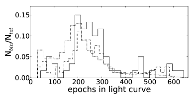
Figure 1.— Normalized histograms of the number of light curve epochs available for each source in the Bright LINEAR catalog. The distributions are shown for 140 blazars (solid), 978 normal quasar (dashed), and all other objects (dotted).

epochs of observation for each of the 140 objects in the blazar sample, the 987 objects in the normal quasar sample, and all other objects (mainly stars) in the Bright LINEAR Catalog. The histograms are all generally consistent with each other, peak at $\sim$200 epochs, and lack objects with $<$30 good observations due to the previously imposed cut.

Before attempting to model the light curve of every object, we would first like to compare the general level of variability of blazars, normal quasars, and other objects in the Bright LINEAR Catalog. We follow Sesar et al. (2007) and estimate the intrinsic rms variability $\sigma$ for each light curve, defined as

$$\sigma=[\Sigma^{2}-\psi(m_{LINEAR})^{2}]^{1/2}$$ (1)

for all objects with $\Sigma$ $>$ $\psi$(m_LINEAR) and $\sigma$ = 0 otherwise, where $\Sigma$ is the rms scatter of the m_LINEAR for all observations of each object, and $\psi$(m_LINEAR) is the median photometric error of LINEAR objects as a function of magnitude found by SE11 (see their Equation 7). Since the photometric errors in LINEAR are relatively large, $\Sigma$ mainly reflects photometric noise rather than variability for the vast majority of objects. Equation 1 attempts to remove the effects of the median photometric error, and thus $\sigma$ is a better measure of intrinsic variability. Figure 2 shows the median $\sigma$ and

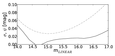
Figure 2.— Median intrinsic rms variability $\sigma$ (solid) and photometric uncertainty $\psi$(m_LINEAR) (dash-dot; Equation 7 from SE11) of LINEAR objects in the Bright LINEAR catalog, as a function of recalibrated LINEAR magnitude.

$\psi$(m_LINEAR ) of all objects in the Bright LINEAR catalog as a function of m_LINEAR magnitude.

We compare the variability of blazars to normal quasars and other LINEAR objects, as it is expected that blazars should be systematically more variable. Figure 3 shows the integrated distribution of blazars,

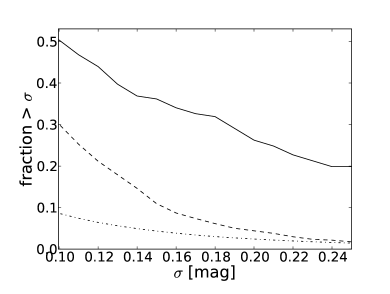
Figure 3.— Fraction of objects with a intrinsic rms variability larger than $\sigma$, as a function of $\sigma$, for blazars (solid), normal quasars (dashed), and other objects (dash-dot).

normal quasars, and other LINEAR bright objects in the Bright LINEAR catalog as a function of the estimated intrinsic rms variability $\sigma$. We estimate that $\sim$36% of blazars, as compared to only $\sim$11% of quasars, are variable with $\sigma$ $>$ 0.15 mag in this passband. At this level of variability, the estimate of $\sigma$ is not significantly affected by uncertainties in $\psi$(m${}_{LINEAR})$. Only $\sim$4% of the other bright LINEAR objects (non-blazars and non-quasars) are variable above this $\sigma$ $>$ 0.15 mag level, and they are likely a combination of variable stars (e.g. RR Lyrae), eclipsing binaries, underestimates of the photometric errors $\psi$, source blending, or other photometric issues.

2.3. The Variable LINEAR catalog

In order to characterize the photometric variability, we need a clean sample of light curves dominated by intrinsic variability rather than photometric errors. Thus, we follow the method of Sesar et al. (2007) to create a clean Variable LINEAR catalog as a subsample of the 4.5 million objects in the Bright LINEAR catalog discussed in the previous section.

As a first variability criterion, we require $\sigma>$ 0.1, roughly equivalent to selecting sources with $\sigma$ more than two times the measurement noise at 14 $<$ m_LINEAR $<$ 16, and roughly corresponding to the photometric error at m${}_{LINEAR}\sim 17$. Approximately 8% of objects in the Bright LINEAR Catalog pass this initial selection cut, including some non-variable objects at the faint end with large $\sigma$ due to large photometric errors. To reduce these spurious contaminants, we assume that the photometric error distribution follows a Gaussian, and place a cut on the $\chi^{2}$ per degree of freedom calculated with respect to a weighted mean magnitude and errors from the photometry. A cut of $\chi^{2}/dof$ $>$ 3 leaves 188,745 objects comprising the Variable LINEAR catalog we use hereafter, each typically having $\sim$200 epochs per light curve.

Matching this variable LINEAR sample to the various catalogs described in Section 2.2 yields 60 blazars and 155 normal quasars, including 1 of the 3 overlapping objects discussed previously in Section 2.2 that we include in both samples. Although the variable LINEAR sample cuts out the majority of the known 140 blazars and 978 normal quasars in the Bright LINEAR catalog, this is not because the majority of blazars and normal quasars are non-variable, but rather because the large photometric errors in LINEAR overwhelm the intrinsic variability of fainter LINEAR objects. This effect can be seen in the much larger fraction of blazars (60 out of 140) that survive these variability cuts, in comparison to normal quasars (155 out of 978). Since blazars tend to be systematically more variable than normal quasars (as we have shown in Section 2.2), their intrinsic variability will dominate over photometric errors for a much larger fraction of objects.

3. The Damped Random Walk Model

MA11 designed and tested optical variability-based selection of quasars in SDSS Stripe 82 by modeling the individual light curves of known quasars as a damped random walk. We perform a similar analysis of the LINEAR light curves of known blazars and normal quasars, and show that blazar light curves lie in a distinct region of DRW variability parameter space. The DRW model statistically parametrizes variability using three parameters: a mean light curve magnitude, a characteristic damping timescale of variability $\tau$, and a driving amplitude of short-term stochastic variability $\hat{\sigma}$ (see Kelly et al., 2009; Kozłowski et al., 2010; MacLeod et al., 2010; Zu et al., 2012, for further discussion). The fitted parameters can be expressed in terms of the structure function (SF), defined as the rms magnitude difference between all pairs of observations in each individual light curve as a function of the time-lag. While this model is phenomenological, it is likely that the fitted parameters reflect the physical processes that cause the variability.

Following Kozłowski et al. (2010) and MA11, we model each individual light curve in our sample as a stochastic process described by the exponential covariance matrix

$$S_{ij}=\sigma^{2}\mathrm{exp}(-|t_{i}-t_{j}|/\tau)$$ (2)

for each pair of observations at time $t_{i}$ and $t_{j}$ in the light curve. This describes a DRW process with a characteristic damping timescale $\tau$ beyond which the structure function will asymptote to a constant value of SF${}_{\infty}=\hat{\sigma}\sqrt{\tau}$, and a long-term standard deviation of variability $\sigma=\sqrt{2}$SF_∞. The short-term driving amplitude of variability $\hat{\sigma}=\sigma\sqrt{2/\tau}$ determines the rise of SF($\Delta\mathit{t}$) for $\Delta$$t\ll\tau$. We model each individual light curve and calculate $\hat{\sigma}$ and $\tau$, along with their likelihood distributions, using the method of Press et al. (1992), its generalization in Rybicki & Press (1992), and the fast computational implementation in Rybicki & Press (1995). The corresponding structure function for the model for time-lag $\Delta t$ is

$$\rm{SF}(\Delta\mathit{t})=\rm{SF}_{\infty}(1-e^{-|\Delta\mathit{t}|/\tau})^{1/2}.$$ (3)

In fitting each individual light curve with the DRW model, we calculate the likelihood of a DRW solution $L_{DRW}$, as well as the likelihood of a pure white noise solution $L_{noise}$. Light curves that are better described by the DRW model than white noise at a 5-sigma level will have $\Delta$$L_{noise}$ = ln($L_{DRW}$/$L_{noise}$) $>$ 5. All our FSRQ and BL Lac object light curves in the Variable LINEAR catalog fit the DRW model at above this 5-sigma level. To remove light curves for which the survey length is shorter than $\tau$ (thus leaving $\tau$ unconstrained), we also calculate the likelihood of a runaway timescale, $L_{\infty}$. Objects for which $\tau$ is constrained in the DRW model will have $\Delta$$L_{\infty}$ $=$ ln($L_{DRW}$/$L_{\infty}$) $>$ 0.05 (MacLeod et al., 2010). MacLeod et al. (2010) showed that the DRW is an excellent fit to quasar light curves, and used cuts on minimum $\Delta$$L_{noise}$ and minimum $\Delta$$L_{\infty}$ to select quasars with high quality light curves. In the higher stellar density regions of Stripe 82, MC11 used cuts on maximum $\hat{\sigma}$, minimum $\tau$, and minimum $\Delta$$L_{noise}$ to achieve impressive completeness $C$ $=$ 93% (defined as percentage of the total confirmed quasars in the sample which are selected) and efficiency $E$ $>$ 78% (percentage of quasar candidates selected which are confirmed quasars) in quasar selection. Furthermore, Kozłowski et al. (2010) showed that the method works even in the high stellar density regions of the Magellanic Cloud fields

We calculate the best-fit DRW variability parameters of the individual light curves of the 60 blazars, 155 normal quasars, and a random sample of 6000 other objects (mainly foreground Galactic stars, representative of the other $>$180,000 objects) from the Variable LINEAR catalog. To first understand the underlying distribution of DRW variability parameters for these different populations, we redshift-correct our parameters as outlined in Kelly et al. (2009) using spectroscopic redshifts from the Schneider et al. (2010) catalog for all FSRQs and normal quasars. For BL Lac objects, redshifts are much less accurate (and sometimes not possible) due to the lack of strong spectral features. Since our sample of BL Lac objects is drawn from a variety of catalogs, there are sometimes discordant redshifts reported; in such cases, we preferentially adopt the spectroscopically derived redshifts (or the lower limits) from the Plotkin et al. (2008) and Plotkin et al. (2010) catalogs. For 3 BL Lac objects, there is no redshift reported in any of the catalogs, and so for these 3 objects we adopt the mean redshift found for all other LINEAR BL Lac objects, $z$ = 0.28. While this assumption is not ideal, very few extragalactic objects in the LINEAR survey will be at high redshifts due to the shallow optical flux limit, so uncertainties on these 3 redshifts will not strongly impact our results.

Imposing the restrictions on $\Delta L_{\infty}>0.05$ and $\Delta L_{noise}>5$ leaves us with 51 blazars and 121 normal quasars in our sample. Figure 4 shows

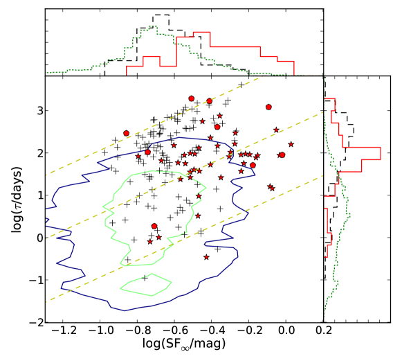
Figure 4.— Distribution of variable LINEAR objects in SF_∞ (asymptotic value of the structure function on long timescales) and $\tau$ (characteristic damping timescale). BL Lac objects (red stars), FSRQs (red circles), normal quasars (black crosses), and contours enclosing 90% (blue) and 50% (green) of all other objects are shown. The side panels show the projected normalized histograms of the distributions in SF_∞ (top) and $\tau$ (right) for blazars (BL Lac objects and FSRQs, red solid), normal quasars (black dashed), and other objects (green dotted). Dashed yellow lines of constant $\hat{\sigma}$ for $\hat{\sigma}$ = $-$0.75, 0.0, 0.75 are also shown, with $\hat{\sigma}$ increasing towards the lower right.

the best-fit DRW parameters $\tau$ against SF_∞ of blazars, normal quasars, and other objects (mostly Galactic stars), along with normalized histograms of their distributions. Although we use separate symbols for BL Lac objects and FSRQs in Figure 4, we do not separate these two blazar sub-populations in our subsequent analysis due to the small sample size and unknown biases in our blazar sample stemming from possible correlations between variability and physical properties of the blazars. Future surveys yielding larger samples may be able to robustly constrain differences between these two sub-populations, and provide further insight into their jet properties. Figure 4 is directly comparable to the analysis of Kozłowski et al. (2010) and MA11, and confirms that the structure functions of normal quasar light curves tend to have longer characteristic timescales of variability $\tau$ and slightly larger SF_∞ than stars. More importantly, our analysis also shows that blazars have characteristic timescales $\tau$ in between those of normal quasars and other objects (mainly variable stars), as well as larger values of SF_∞. The driving amplitude on short timescales $\hat{\sigma}$, is related to these two parameters by the relation $\hat{\sigma}$ = SF_∞/$\sqrt{\tau}$, as shown in Figure 4. Figure 5 shows the distribution for blazars and normal quasars in

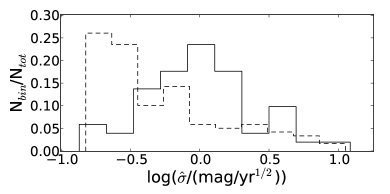
Figure 5.— Distributions of the driving amplitude on short timescales $\hat{\sigma}$ for blazars (solid), and normal quasars (dashed) in the Variable LINEAR catalog.

$\hat{\sigma}$, where normal quasars tend to peak at log ($\hat{\sigma}$/mag yr^-1/2) $\sim-0.75$, while blazars tend to peak at log $\hat{\sigma}$ $\sim 0.0$. A two-dimensional Kolmogorov-Smirnoff test between the distributions of $\hat{\sigma}$ for blazars and normal quasars in Figure 5 gives a p-value of $2.04\times 10^{-5}$. For the distributions of $\tau$ in Figure 4, the p-value is 0.032.

While MA11 performed quasar selection using this approach by placing cuts on maximum $\hat{\sigma}$ and minimum $\tau$, we can also see from Figure 4 that a minimum $\tau$ cut would separate blazars from other objects (mostly Galactic stars), while a minimum $\hat{\sigma}$ cut can help separate blazars from quasars. However, it is clear from Figure 4 that highly efficient and complete quasar and blazar selection purely by optical variability in the LINEAR survey is difficult, as there will be either be heavy contamination or a low recovery rate. The main cause of this is the bright magnitude range (14 $<$ m_LINEAR $<$ 17) of LINEAR, which overwhelmingly probes Galactic stars and very few actual AGN (e.g. there are $>$180,000 sources in the Variable LINEAR catalog, only 214 of which are known normal quasars and blazars), and so deeper survey data containing a substantial fraction of extragalactic sources is necessary. However, currently available data from deeper time-domain optical surveys such as SDSS Stripe 82 have comparatively small sky coverage, and do not yield a large enough sample of the much rarer blazars.

4. Blazar Selection in Fermi Error Circles

Despite the overwhelming stellar contamination in the bright magnitude range of the LINEAR survey, our proposed blazar selection method is still useful with LINEAR if we restrict our search to the small regions of sky associated with the positions of Fermi sources. This greatly reduces the stellar contamination, while simultaneously providing a test of a novel method (based on long-term photometric variability characteristics) to associate $\gamma$-ray sources with counterparts at optical wavelengths. We will show the DRW parameters of known Fermi AGN (overwhelmingly blazars), quantify the completeness and efficiency of blazar selection using this method, and identify new variability-selected candidate Fermi blazar counterparts.

We first positionally match the Variable LINEAR catalog described in Section 2.3 to the 1873 sources in the 2FGL catalog, approximating each error ellipse as a circle with radius equal to the semi-major axis of the 95% confidence ellipse. This initial match yields 480 variable LINEAR objects in 173 Fermi error circles. These 480 variable LINEAR optical objects in Fermi error circles are then positionally matched using a $3\farcs 0$ matching radius to the 929 associated AGN in the 2nd Fermi AGN catalog (Ackermann et al., 2011), restricting consideration to those that have Bayesian association probabilities $>$0.8 (this association method is described in the Appendix of Abdo et al., 2010). This yields a sample of 47 known (i.e. confidently associated) Fermi $\gamma$-ray emitting AGN. We calculate DRW parameters for the LINEAR light curves of all 480 variable objects, and make nominals cut on $\Delta L_{noise}$ $>$ 5 and $\Delta$$L_{\infty}$ $>$ 0.05 as in Section 3.

Due to the bright magnitude range of the LINEAR survey, it is likely that the flux limit of the LINEAR survey is too bright to actually detect the optical counterparts of the faintest Fermi $\gamma$-ray sources, leaving us a population of orphan error circles which contain only LINEAR contaminants. Since these fainter sources will also preferentially have larger error circles, we can remove them by considering further cuts on the maximum radii of the error circles. In Figure 6, we show the distribution of the

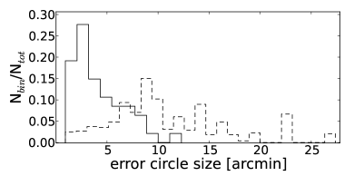
Figure 6.— Distribution of the number of variable LINEAR objects lying in all Fermi error circles of radius $r$ (dashed), and only those lying in Fermi error circles of radius $r$ which contain a variable LINEAR object matched to an AGN in the 2nd Fermi AGN catalog (solid), as a function of $r$.

total number of LINEAR variable objects in Fermi error circles as a function of error circle radius $r$, for all 173 error circles that contain at least 1 LINEAR variable object, as well as the distribution for the 47 error circles containing a LINEAR variable object that matched to an AGN in the 2nd Fermi AGN catalog. Figure 6 shows that the number of variable LINEAR objects in error circles with known $\gamma$-ray AGN counterparts peaks at $2\arcmin$ and drops rapidly; beyond $10\arcmin$, there is only 1 Fermi error circle that contains a known $\gamma$-ray AGN counterpart. However, the distribution of the total number of variable LINEAR objects in all error circles as a function of radius has a long tail to large $r$, as there are a small number of large error circles ($r>15\arcmin$) with large numbers of variable LINEAR objects, as expected. This suggests that a cut on the error circle radius of $\sim$$10\arcmin$ is appropriate, but to gauge the impact of such a cut, we will in detail consider a range of $8\arcmin$, $10\arcmin$ and $12\arcmin$ cuts on the maximum error circle size. A cut at $r<10\arcmin$ removes from consideration only 1 Fermi error circle containing a known $\gamma$-ray AGN, while a cut at $r<8\arcmin$ removes 4. Scatter in the negative relation between the optical flux and $\gamma$-ray error circle size of Fermi blazars may introduce some biases in our resulting sample towards blazars with higher than average optical to $\gamma$-ray flux ratios when we place a cut on the error circle size. However, this bias is expected to be small, as only $\sim$7% of reliably associated AGN in the 2nd Fermi AGN Catalog with optical magnitudes $<$17 reside in Fermi error circles $>$10$\arcmin$ in radius. We note that although the Fermi AGN association success rate of Ackermann et al. (2011) as a function of $r$ will also affect Figure 6, this effect is secondary to the LINEAR flux limit for the high association probabilities considered here.

Figure 7 (left panel) shows the distribution in $\tau$ and SF_∞

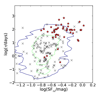
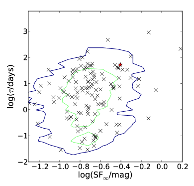
Figure 7.— Left: Distribution of variable LINEAR objects in Fermi error circles of radius $r<10\arcmin$, in SF_∞ and $\tau$, for reliably associated Fermi AGN (red stars), and other objects (black crosses). The underlying contours from Figure 4 enclosing 90% (blue) and 50% (green) of all other objects in the Variable LINEAR catalog is shown in the background for reference. Right: Same as the left panel, but for Fermi error circles $>$$10\arcmin$ in radius.

of LINEAR optical counterparts to Fermi $\gamma$-ray AGN, as well as all other variable objects in Fermi 2FGL error circles of $r<10\arcmin$. We do not apply cosmological redshift-corrections here for blazar selection. Similar to the conclusions drawn from Figure 4, there is clear separation between $\gamma$-ray emitting AGN and other LINEAR variables in DRW parameter space. The significant normal quasar population seen in Figure 4 is minimized when looking only in Fermi error circles. As expected, almost all $\gamma$-ray AGN recovered in our sample have blazar-like variability. Figure 7 (right panel) shows that variable objects in error circles with radius $r>10\arcmin$ largely have SF_∞ and $\tau$ similar to that of stars, and are thus mostly contaminants, rather than new blazar candidates which were removed by the cut on $r<10\arcmin$.

We can select $\gamma$-ray AGN by placing cuts on minimum $\tau$ and $\hat{\sigma}$. For different log $\tau$ and log $\hat{\sigma}$, we estimate efficiency and completeness of $\gamma$-ray AGN selection. The results for a $10\arcmin$ cut on the error circles are shown in Figure 8. Selection cuts at large

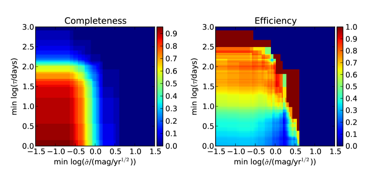
Figure 8.— Completeness and efficiency of selection of confirmed Fermi AGN in error circles of radius $r<10\arcmin$, as a function of selection cuts on minimum $\tau$ and $\hat{\sigma}$ .

minimum $\tau$ and minimum $\hat{\sigma}$ yield efficiencies of 0 as there are no such objects. Figure 9

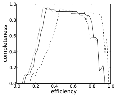
Figure 9.— Maximum completeness achievable for a given efficiency of selection, for confirmed Fermi AGN in error circles of radius $r<8\arcmin$ (dashed), $r<10\arcmin$ (solid), and $r<12\arcmin$ (dotted) as a function of efficiency.

shows the maximum completeness achievable by tweaking the selection cuts on minimum $\tau$ and $\hat{\sigma}$, as a function of efficiency. This shows how the completeness changes as a function of efficiency in $\gamma$-ray AGN selection, for error circles with a maximum radius of $8\arcmin$, $10\arcmin$, and $12\arcmin$. As expected, the efficiency decreases as the maximum size of error circles considered increases, at a set completeness.

By jointly maximizing efficiency and completeness via the quantity $\sqrt{E^{2}+C^{2}}$ from the curves in Figure 9, we can achieve $E$ $\geq$ 88% and $C$ $=$ 88% for Fermi error circles of $r<8\arcmin$ using cuts on log $\tau>1.35$ and log $\hat{\sigma}>-1.20$. For error circles of $r<10\arcmin$, $E$ $\geq$ 76% and $C$ $=$ 86% using cuts on log $\tau>1.53$ and log $\hat{\sigma}>-0.90$, and for error circles of $r<12\arcmin$, $E$ $\geq$ 70% and $C$ $=$ 86% using cuts on log $\tau>1.53$ and log $\hat{\sigma}>-0.90$. This demonstration verifies that we are able to select (in this case, recover in double-blind fashion) $\gamma$-ray emitting AGN in Fermi error circles with high completeness and efficiency by modeling their optical light curves as a DRW, and imposing selection cuts on the variability parameters.

Our definition for completeness is similar to the convention of many other recent time-domain AGN studies (e.g. MA11). The completeness we calculate here is specifically for the selection of variable LINEAR objects matched to Fermi AGN in Ackermann et al. (2011) with Bayesian association probabilities $>$0.8, and the efficiency is calculated assuming these associations are all correct. However, this efficiency is a lower bound, as it will increase if some of the contaminants we encounter in selection are actually blazars. This may occur in our analysis if some LINEAR variables that pass all DRW blazar selection cuts and did not match to a AGN in the 2nd Fermi AGN catalog may actually be additional $\gamma$-ray AGN counterparts, not already recognized as such. Indeed, this is likely the case for at least one object, lying in the error circle of Fermi source 2FGL J1649.6+5238.

In the 2nd Fermi AGN catalog, Fermi source 2FGL J1649.6+5238 is listed as associated with the radio source 87GB 164812.2+524023 at a 0.0 Bayesian probability, calculated based on the local density of sources from catalogs of likely counterparts. This radio source is positionally coincident with a LINEAR object at RA = 16^h49^m24^s.99, Dec = 52^∘35$\arcmin$15$\arcsec$.05, which has DRW parameters calculated from its LINEAR light curve of log $\tau$ = 1.936, log $\hat{\sigma}=-0.026$, and log SF_∞ = 0.942, very similar to that of confirmed $\gamma$-ray AGN in Figure 7. This LINEAR source was not counted as a $\gamma$-ray AGN in our calculations of efficiency and completeness because its Bayesian probability of association was below 0.8 in Ackermann et al. (2011). Furthermore, this LINEAR counterpart also did not match to any known blazar in the BL Lac object and quasar catalogs used in Section 2.2.

Based on these blazar-like DRW parameters calculated from the light curve, we suggest this LINEAR variable object as the plausible optical counterpart to Fermi source 2FGL J1649.6+523, as well as increased confidence in associating 87GB 164812.2+524023 as the radio counterpart. We note that this Fermi source is also associated with this radio source with a 0.82 probability using the $\log N$–$\log S$ method in Ackermann et al. (2011), based on observed properties of candidate radio counterparts. The origin of this disparity lies in the differences in the approaches used to calculate the Bayesian and $\log N$–$\log S$ (radio) association probabilities. We opted to use the Bayesian probability $>$0.8 criterion for known $\gamma$-ray AGN, but the use of the $\log N$–$\log S$ probability also recovers this radio source as a likely $\gamma$-ray AGN. It is not our intention to compare the two statistical approaches, but rather to point out that the discrepancies in the results of these two methods may lead to different results in analysis. In cases where these two methods lead to highly discrepant results, our completely independent optical variability-based method can provide valuable additional information.

Finally, we note that our variability-based approach may be further applicable to mass identification of unassociated $\gamma$-ray sources using deeper time-domain optical surveys. Data from current surveys such as the PTF, with single-epoch depth of $r\sim 20.6$ mag, 30 epochs of observation over 8,200 deg² of sky, and $\sim$0.01 mag repeatability can be used to identify unassociated Fermi blazars using the method we have presented here. Future surveys such as LSST, with single-epoch depth of $r\sim$ 24.5 mag over 20,000 deg² of sky and $\sim 10^{3}$ epochs per source can be used to vastly increase the existing sample size.

5. Discussion

5.1. Efficiency and Completeness

In Section 3, we noted that blazar selection using the Variable LINEAR catalog across the full field of the survey (as contrasted to blazar selection only within Fermi error circles) was not efficient and complete. At first, this may seem to be in stark contrast to the success of quasar variability selection using a similar DRW modeling approach (e.g., MA11, Butler & Bloom, 2011; Kozłowski et al., 2010). This is primarily a consequence of the shallow depth of the LINEAR survey rather than a reflection of the ultimate performance expected from our approach (especially for fainter blazars). At the depth of SDSS Stripe 82 (flux limit of $g\sim 20.5$), objects with low-redshift quasar-like colors account for $\sim$63% of all variable objects, with Galactic stars making up the vast majority of the remaining variable objects (Sesar et al., 2007). In contrast, at the shallow depth of the LINEAR survey (flux limit of $r\sim 17$), only $\sim$0.08% of objects in the variable LINEAR catalog are quasars (see Section 2.3). As such, quasar selection by imposing appropriate maximum $\hat{\sigma}$ and minimum $\tau$ cuts (as done in MA11) on the LINEAR quasar sample in Figure 4 will not yield $E$ beyond a few percent for any value of $C$ $>$ 50% due to scatter in the parameters of the enormously larger population of variable stars. Blazar selection in LINEAR will be similarly inefficient. These issues are exacerbated by the large errors on the estimated DRW parameters as compared to SDSS, caused by the larger photometric uncertainties in LINEAR. In any case, current and future time-domain surveys such as PTF and LSST will alleviate both these issues by going many magnitudes deeper while providing $\sim$1% photometry.

As noted in Section 4, our calculated efficiencies of blazar selection are lower limits, since calculating the true efficiency requires correct identification of every object as either a blazar or contaminant. There are many contaminating variable LINEAR objects that fall in the Fermi error circles we considered in our analysis in Section 4 that have blazar-like variability (i.e. have DRW parameters similar to blazars and are counted as contaminants when jointly optimizing completeness and efficiency for known $\gamma$-ray blazar selection). Some of these contaminants are certainly blazars, and may actually be the $\gamma$-ray source. Securing identification of these blazar-like variable objects will require spectroscopic follow-up. We list in Table 1 the positions, parent 2FGL error circle, and DRW parameters of 12 such new candidate LINEAR variable objects with blazar-like optical variability that fall in Fermi 2FGL error circles with $r<10\arcmin$. We also list any previously-associated counterparts of each parent 2FGL source from Ackermann et al. (2011) with Bayesian association probabilities $>$0.8. The LINEAR blazar candidates are not positionally coincident with these previously-associated counterparts, but are rather additional $\gamma$-ray blazar candidates in their respective error circles. Since it is possible that some Fermi error circles may contain more than one $\gamma$-ray emitting object, these LINEAR blazar candidates are still worthy of spectroscopic follow-up.

Table 1J2000 Positions of new candidate LINEAR blazars in Fermi error circles with $r<10\arcmin$ selected by variability

RA (degrees)	Dec (degrees)	Fermi 2FGL Source	log($\tau$/days)	log($\hat{\sigma}$/(mag yr-1/2))	2nd Fermi AGN Catalog Association
$128.5027$	$42.2570$	2FGL J0834.3+4221	$1.89$	$-0.20$	OJ 45
$153.3687$	$34.4883$	2FGL J1013.6+3434	$1.58$	$-0.28$	unassociated
$172.2141$	$-5.6568$-	2FGL J1129.0$-$0532	$2.20$	$-$$0.02$	unassociated
$189.5802$	$-20.0237$$-$	2FGL J1238.1$-$1953	$2.07$	$-0.11$	PMN J1238-1959
$219.1272$	$23.2824$	2FGL J1436.9+2319	$1.66$	$-0.29$	PKS B1434+235
$220.4843$	$43.9407$	2FGL J1442.0+4352	$2.00$	$-0.26$	BZB J1442+4348
$232.8992$	$57.4483$	2FGL J1531.0+5725	$2.50$	$-0.04$	unassociated
$232.9009$	$57.3541$	2FGL J1531.0+5725	$2.36$	$-0.58$	unassociated
$246.9883$	$32.4363$	2FGL J1627.8+3219	$2.30$	$-0.34$	unassociated
$250.2259$	$11.7870$	2FGL J1641.0+1141	$1.89$	$-0.20$	MG1 J164058+1144
$252.3542$	$52.5875$	2FGL J1649.6+5238	$1.93$	$-0.02$	unassociated
$331.7412$	$-0.4681$-	2FGL J2206.6$-$0029	$1.80$	$-$$0.27$	PMN J2206-0031

We further note that the efficiencies we have calculated in $\gamma$-ray blazar selection in Section 4 are conservative, as we have considered all variable LINEAR objects lying in all Fermi error circles below a certain size. However, $\sim$10% of sources in the 2FGL are associated with non-AGN objects (e.g. pulsars, supernovae remnants, etc.), while $\sim$30% of sources are unassociated. We chose to include all these error circles in our analysis (and not just those containing known Fermi blazars) in a double-blind test, as it is a more faithful demonstration of the efficacy of this approach.

We would like to compare the efficiency and completeness of our variability-based Fermi blazar selection method to other methods. However, a direct comparison is difficult; few studies have attempted to use characteristic properties of blazars to systematically select Fermi blazars in double-blind fashion as we have done. Furthermore, the completeness and efficiency of those methods are almost never jointly optimized (as done in Section 4). For example, Massaro et al. (2011) used mid-IR color selection to recover known blazars in the WISE survey, and extended their approach to find new Fermi blazar candidates (Massaro et al., 2012). By parametrizing the similarity of the mid-IR colors of WISE sources to WISE-detected Fermi blazars, Massaro et al. (2012) imposed a mid-IR color-based selection criterion that is able to select known Fermi blazars with 87% completeness over the full region of sky surveyed by WISE in its first year. However, Massaro et al. (2012) did not jointly calculate the completeness and efficiency of their approach. Their mid-IR color selection method has the advantage of the all-sky coverage of the WISE survey. However, mid-IR color selection is dependent on the degree to which non-thermal jet emission dominates the mid-IR emission of individual blazars. Indeed, Massaro et al. (2011) find that FSQRs generally have WISE colors closer to normal quasars than to BL Lac objects. This may be due to significant thermal mid-IR emission in the SEDs of FSRQs, similar to that in normal quasars (e.g. from dust emission, see Plotkin et al., 2012), thus making blazar selection more difficult.

Massaro et al. (2012) apply their selection method to WISE sources in unidentified Fermi error circles to find 297 $\gamma$-ray blazar candidates in 156 out of 313 unidentified Fermi error circles. However, their estimates of the efficiency of their method by systematically offsetting the position of each Fermi error circle to assess the number of random associations gave 262 false blazar candidates (using the same mid-IR color selection criteria), suggesting that the efficiency of this approach may be low. Nevertheless, mid-IR color- and variability-based selection of blazars are independent and complementary methods, with different selection biases. A combination of both approaches, using the full WISE survey as well as data from current time-domain optical imaging surveys, may be highly efficient and complete.

5.2. Implications for Blazar Variability

Our finding that optical blazar variability is well described as a DRW process with distinct variability parameters may have interesting potential implications for blazar jet physics. The SF_∞ and $\tau$ DRW parameters should both be affected by relativistic effects. For example, the observed blazar characteristic damping timescale $\tau_{blz,obs}$ (after correcting for cosmological redshift) should be shortened in comparison to the interval $\tau_{blz,rest}$ in the rest-frame of the emitting material due to the relativistic motion, with $\tau_{blz,rest}$ = $\delta\tau_{blz,obs}$, where $\delta$ is the kinematic Doppler factor. While $\tau_{blz,rest}$ is uncertain and difficult to measure, we can place constraints on it through comparisons to $\tau_{qso}$, the characteristic DRW timescale of normal quasars (which are not affected by relativistic effects), and independent measurements of $\delta$.

In Figure 4, the distributions of $\tau$ peaks at $\tau_{blz,obs}\sim 80$ days for blazars, and $\tau_{qso}\sim 320$ days for normal quasars. While these distributions have large tails, their relative peaks provide an adequate basis for comparison. If the underlying variability in quasars ultimately also drives blazar variability, then $\delta\sim\tau_{qso}/\tau_{blz,obs}\sim$ 4. Figure 10 shows the distribution of this estimated

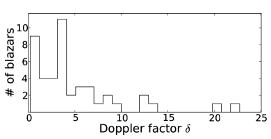
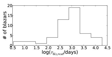
Figure 10.— $Top$: Distribution of calculated kinematic Doppler factors of blazars in the Variable LINEAR catalog, assuming that the rest-frame characteristic timescale of variability for each blazar is equal to that of LINEAR normal quasars (320 days). $Bottom$: Distribution of calculated rest-frame characteristic timescale of variability for blazars in the Variable LINEAR catalog, assuming a kinematic Doppler factor $\delta=10$.

$\delta$ for blazars in the Variable LINEAR catalog, assuming $\tau_{qso}=320$ days. This is smaller than estimates of the typical blazar Doppler factor from radio observations of Fermi-detected blazars ($\delta\sim$ 10 - 30, Savolainen et al., 2010), and may imply that the variability of the non-thermal jet emission in the jet rest-frame (e.g. due to shocks in the jet) occurs on longer timescales than the thermal disk variability of normal quasars.

We can instead adopt the observed typical Doppler factors for blazars and calculate $\tau_{blz,rest}$ for each individual blazar. Ideally, we would use a measured value of $\delta$ for each individual blazar in this calculation, but direct measurements of $\delta$ from the literature are sparse and inhomogeneous. In Figure 10 (bottom panel), we show the distribution of $\tau_{blz,rest}$ assuming a reasonable $\delta=10$ for all blazars. The peak in Figure 10 occurs at $\tau_{blz,rest}\sim 3$ years, which is longer than the $\tau_{qso}\sim$ 320 days we measure for LINEAR normal quasars. The discrepancy between $\delta$ for Fermi blazars implied by radio observations and $\delta$ calculated assuming intrinsic variability similar to normal quasars suggests different stochastic mechanisms driving the variability in the disk and the jet. While a detailed physical interpretation of this is currently unclear, our long-term optical variability results may provide additional constraints on models of blazar jets.

5.3. Short Timescale Variability of Quasars and Blazars

Observations of intraday variability (also referred to as ‘microvariabilty’) of normal quasars have shown a puzzling diversity of properties. Not all quasars exhibit this phenomenon, but some show variability on the order of $\sim$0.01 mag on $\sim$1 day timescales (Gopal-Krishna et al., 2003; Stalin et al., 2004, 2005; Gupta & Joshi, 2005; Mushotzky et al., 2011). The cause of quasar variability on such short timescales is an unresolved problem, although the presence of strong intraday variability is correlated with radio-loudness, and it has long been suspected that a weak jet component may be both the source of radio emission and the cause of the stronger variability. Kelly et al. (2009) showed that the DRW model successfully predicts amplitudes of variability of $\lesssim$0.02 mag over $\sim$8 hours for quasars, consistent with observations from quasar monitoring. This successful prediction of the short-timescale variability is noteworthy since the sampling intervals of the quasar light curves used in Kelly et al. (2009) are all $\geq$2 days, and thus do not actually sample such intraday timescales.

From the log $\hat{\sigma}$ distributions for normal quasars and blazars in Figure 5, we can calculate the standard deviation of the expected variability on $\sim$1 day timescales, approximated as $\hat{\sigma}$$\sqrt{\Delta t}$. For quasars, the peak of the distribution occurs at $\sim$0.2 mag yr^-1/2, thus predicting intraday variability $\sim$0.01 mag on 1 day timescales. For blazars, the peak occurs at $\sim$1 mag yr^-1/2, thus predicting variability of $\sim$0.05 mag on 1 day timescales in the observed frame. Previous studies of blazar microvariability have often focused on the most variable blazars, and have reported night-to-night variations as high as 1.0 mag (e.g. Carini et al., 1991; Ghosh et al., 2000). The intraday variability we have calculated for LINEAR blazars is from an untargeted (i.e. less biased) survey, and is likely more representative of the intraday variability of blazars as a whole.

Despite the large photometric uncertainties in the LINEAR survey, there are a significant number of normal quasars and blazars in Figure 5 which do have extreme levels of short-timescale variability, above the photometric uncertainty. Nearly all LINEAR objects have photometric uncertainties below 0.1 mag (and reaching as low as $\leq$0.04) at $<$17 mag (see Figure 2). Conservatively assuming that variability on 1 day timescales needs to be $>$0.1 mag in order to be detectable above the photometric uncertainty implies a log $\hat{\sigma}$ $>$ 0.28. In Figure 5, 18 of 119 normal quasars and 10 of 51 blazars in our sample are variable above this criterion (and both these fractions would increase if we more carefully considered the photometric uncertainty limit of each individual object). Thus for these objects, the intraday variability is above the LINEAR photometric uncertainty and the $>$0.1 mag intraday variability is significantly above most previous observations of normal quasars. The source of this extreme variability for a subset of quasars is unknown, and warrants additional investigation.

6. Conclusions

We have used light curves from the LINEAR optical imaging survey to study the variability of blazars, and to compare their variability to that of normal quasars. In contrast to many earlier studies of blazar variability, this study is the first to use a reasonably large, homogeneous sample of individual light curves from a wide-field survey, where the distribution of various variability properties for blazars and quasars can be calculated and compared.

In a time-domain survey, blazars are among the most violently variable objects detected, and are generally more variable than normal quasars. We estimate that $\sim$36% of blazars but only $\sim$11% of quasars are variable at the extreme $>$0.15 mag intrinsic rms variability level. We show that, like quasars, blazar light curves are well-fit by the DRW model for variability, but the blazars lie in distinct variability parameter-space with higher $\tau$ than stars and higher $\hat{\sigma}$ than normal quasars. This suggests that blazars can be selected with high efficiency $E$ and completeness $C$ by imposing minimum selection cuts on $\tau$ and $\hat{\sigma}$.

Due to the overwhelming numbers of variable stars in the bright magnitude regime probed by LINEAR, it is difficult to select blazars (and quasars) at high efficiency and completeness in the full LINEAR sample using optical variability methods alone. We instead examine a more focused test to select $\gamma$-ray emitting blazars in Fermi error ellipses from the 2FGL catalog. We calculate DRW parameters for light curves of all LINEAR variable objects objects within Fermi error ellipses and place minimum selection cuts on $\tau$ and $\hat{\sigma}$. Using this approach, we are able to recover the corresponding $\gamma$-ray emitting AGN counterparts in the 2nd Fermi AGN catalog with $E$ $\geq$ 88% and $C$ $=$ 88% for 95% confidence error ellipses with semimajor axis $r<8\arcmin$, and $E$ $\geq$ 70% and $C$ $=$ 86% for $r<12\arcmin$.

Our $\gamma$-ray blazar selection has uncovered a variable LINEAR object, coincident with radio source 87GB 164812.2+524023, in the error ellipse of Fermi source 2FGL J1649.6+5238. This object was not associated with the Fermi source in the 2nd Fermi AGN catalog using Bayesian probabilities. Our analysis shows this object has optical variability properties consistent with $\gamma$-ray emitting blazars and is likely to be the $\gamma$-ray source. We find a total of 12 objects with LINEAR variability parameters similar to blazars lying in Fermi error circles with $r<10\arcmin$ (see Table 1). Confirmation of these variability-selected blazar candidates will require spectroscopic follow-up.

Our results suggest that the variability of the non-thermal jet emission in blazars is stochastic in nature, with higher amplitudes and shorter observed timescales in comparison to the variability of normal quasars, likely due to the effects of relativistic beaming. Assuming a reasonable Doppler factor of 10, we estimate that blazars are characteristically variable on timescales of $\sim$3 years in the rest-frame of the emitting material, longer than the $\sim$320 days characteristic disk flux timescale for quasars. This suggests that different physical mechanisms dominate the observed variability from blazars and quasars, likely connected to the jet and to the disk, respectively. The fitted parameters imply that blazars have a typical intraday variability amplitude of $\sim$0.05 mag, compared to $\sim$0.01 mag for normal quasars. Furthermore, there is a significant fraction ($\sim$15%) of normal quasars which exhibit large intraday variability of $>$0.1 mag, detectable above the photometric uncertainty. The source of the extreme variability of these quasars is unclear.

We argue that variability-based blazar selection is likely to be highly efficient and complete in deeper optical time-domain imaging surveys, and that the variability-based blazar selection method presented in this paper is capable of greatly increasing the number of known blazars. Our approach, based on long-term photometric variability characteristics of a large sample of individual blazar light curves, may also bring a new perspective on accretion disk and jet physics. Finally, this work typifies the fruitful ancillary science made possible by combining data from surveys as diverse in all respects as LINEAR, SDSS, and Fermi.

References

- Ackermann et al. (2011) Ackermann, M., Ajello, M., Allafort, A., et al. 2011, ApJ, 743, 171
- Ackermann et al. (2012) Ackermann, M., Ajello, M., Allafort, A., et al. 2012, ApJ, 753, 83
- Abdo et al. (2010) Abdo, A. A., Ackermann, M., Ajello, M., et al. 2010, ApJS, 188, 405
- Atwood et al. (2009) Atwood, W. B., Abdo, A. A., Ackermann, M., et al. 2009, ApJ, 697, 1071
- Barron et al. (2008) Barron, J. T., Stumm, C., Hogg, D. W., Lang, D., & Roweis, S. 2008, AJ, 135, 414
- Bauer et al. (2009a) Bauer, A., Baltay, C., Coppi, P., et al. 2009a, ApJ, 699, 1732
- Bauer et al. (2009b) Bauer, A., Baltay, C., Coppi, P., et al. 2009b, ApJ, 705, 46
- Blandford & Rees (1978) Blandford, R. D., & Rees, M. J. 1978, BL Lac Objects, 328
- Böttcher & Dermer (2010) Böttcher, M., & Dermer, C. D. 2010, ApJ, 711, 445
- Burke et al. (1998) Burke, B. E., Gregory, J. A., Mountain, R. W., et al. 1998, Experimental Astronomy, 8, 31
- Butler & Bloom (2011) Butler, N. R., & Bloom, J. S. 2011, AJ, 141, 93
- Carini et al. (1992) Carini, M. T., Miller, H. R., Noble, J. C., & Goodrich, B. D. 1992, AJ, 104, 15
- Carini et al. (1991) Carini, M. T., Miller, H. R., Noble, J. C., & Sadun, A. C. 1991, AJ, 101, 1196
- Drake et al. (2009) Drake, A. J., Djorgovski, S. G., Mahabal, A., et al. 2009, ApJ, 696, 870
- Gopal-Krishna et al. (2003) Gopal-Krishna, Stalin, C. S., Sagar, R., & Wiita, P. J. 2003, ApJ, 586, L25
- Ghosh et al. (2000) Ghosh, K. K., Ramsey, B. D., Sadun, A. C., & Soundararajaperumal, S. 2000, ApJS, 127, 11
- Gupta & Joshi (2005) Gupta, A. C., & Joshi, U. C. 2005, A&A, 440, 855
- Healey et al. (2007) Healey, S. E., Romani, R. W., Taylor, G. B., et al. 2007, ApJS, 171, 61
- Ivezić et al. (2008) Ivezić, Ž., Tyson, J. A., Allsman, R., Andrew, J., Angel, R., & for the LSST Collaboration 2008, arXiv:0805.2366
- Kaiser et al. (2010) Kaiser, N., Burgett, W., Chambers, K., et al. 2010, Proc. SPIE, 7733,
- Kara et al. (2012) Kara, E., Errando, M., Max-Moerbeck, W., et al. 2012, ApJ, 746, 159
- Kelly et al. (2009) Kelly, B. C., Bechtold, J., & Siemiginowska, A. 2009, ApJ, 698, 895
- Kozłowski et al. (2010) Kozłowski, S., Kochanek, C. S., Udalski, A., et al. 2010, ApJ, 708, 927
- Lacy et al. (2004) Lacy, M., Storrie-Lombardi, L. J., Sajina, A., et al. 2004, ApJS, 154, 166
- MacLeod et al. (2010) MacLeod, C. L., Ivezić, Ž., Kochanek, C. S., et al. 2010, ApJ, 721, 1014
- MacLeod et al. (2011) MacLeod, C. L., Brooks, K., Ivezić, Ž., et al. 2011, ApJ, 728, 26 (MA11)
- Maeda et al. (2011) Maeda, K., Kataoka, J., Nakamori, T., et al. 2011, ApJ, 729, 103
- Massaro et al. (2011) Massaro, F., D’Abrusco, R., Ajello, M., Grindlay, J. E., & Smith, H. A. 2011, ApJ, 740, L48
- Massaro et al. (2012) Massaro, F., D’Abrusco, R., Tosti, G., Ajello, M., & Gasparrini, A. P. D. 2012, arXiv:1203.3801
- Mushotzky et al. (2011) Mushotzky, R. F., Edelson, R., Baumgartner, W., & Gandhi, P. 2011, ApJ, 743, L12
- Nolan et al. (2012) Nolan, P. L., Abdo, A. A., Ackermann, M., et al. 2012, ApJS, 199, 31
- Plotkin et al. (2008) Plotkin, R. M., Anderson, S. F., Hall, P. B., et al. 2008, AJ, 135, 2453
- Plotkin et al. (2010) Plotkin, R. M., Anderson, S. F., Brandt, W. N., et al. 2010, AJ, 139, 390
- Plotkin et al. (2012) Plotkin, R. M., Anderson, S. F., Brandt, W. N., et al. 2012, ApJ, 745, L27
- Press et al. (1992) Press, W. H., Rybicki, G. B., & Hewitt, J. N. 1992, ApJ, 385, 404
- Rau et al. (2009) Rau, A., Kulkarni, S. R., Law, N. M., et al. 2009, PASP, 121, 1334
- Rybicki & Press (1992) Rybicki, G. B., & Press, W. H. 1992, ApJ, 398, 169
- Rybicki & Press (1995) Rybicki, G. B., & Press, W. H. 1995, Physical Review Letters, 74, 1060
- Savolainen et al. (2010) Savolainen, T., Homan, D. C., Hovatta, T., et al. 2010, A&A, 512, A24
- Schneider et al. (2010) Schneider, D. P., Richards, G. T., Hall, P. B., et al. 2010, AJ, 139, 2360
- Sesar et al. (2007) Sesar, B., Ivezić, Ž., Lupton, R. H., et al. 2007, AJ, 134, 2236
- Sesar et al. (2011) Sesar, B., Stuart, J. S., Ivezić, Ž., et al. 2011, AJ, 142, 190 (SE11)
- Stephen et al. (2010) Stephen, J. B., Bassani, L., Landi, R., et al. 2010, MNRAS, 408, 422
- Stalin et al. (2004) Stalin, C. S., Gopal-Krishna, Sagar, R., & Wiita, P. J. 2004, MNRAS, 350, 175
- Stalin et al. (2005) Stalin, C. S., Gupta, A. C., Gopal-Krishna, Wiita, P. J., & Sagar, R. 2005, MNRAS, 356, 607
- Stern et al. (2005) Stern, D., Eisenhardt, P., Gorjian, V., et al. 2005, ApJ, 631, 163
- Stokes et al. (2000) Stokes, G. H., Evans, J. B., Viggh, H. E. M., Shelly, F. C., & Pearce, E. C. 2000, Icarus, 148, 21
- Ulrich et al. (1997) Ulrich, M.-H., Maraschi, L., & Urry, C. M. 1997, ARA&A, 35, 445
- Urry & Padovani (1995) Urry, C. M., & Padovani, P. 1995, PASP, 107, 803
- Véron-Cetty & Véron (2010) Véron-Cetty, M.-P., & Véron, P. 2010, A&A, 518, A10
- Webb et al. (1988) Webb, J. R., Smith, A. G., Leacock, R. J., et al. 1988, AJ, 95, 374
- Wright et al. (2010) Wright, E. L., Eisenhardt, P. R. M., Mainzer, A. K., et al. 2010, AJ, 140, 1868
- York et al. (2000) York, D. G., Adelman, J., Anderson, J. E., Jr., et al. 2000, AJ, 120, 1579
- Zu et al. (2012) Zu, Y., Kochanek, C. S., Kozłowski, S., & Udalski, A. 2012, arXiv:1202.3783