The Maximum Traveling Salesman Problem with Submodular Rewards

Abstract

In this paper, we look at the problem of finding the tour of maximum reward on an undirected graph where the reward is a submodular function, that has a curvature of $\kappa$, of the edges in the tour. This problem is known to be NP-hard. We analyze two simple algorithms for finding an approximate solution. Both algorithms require $O(|V|^{3})$ oracle calls to the submodular function. The approximation factors are shown to be $\frac{1}{2+\kappa}$ and $\max\left\{\frac{2}{3(2+\kappa)},\frac{2}{3}(1-\kappa)\right\}$, respectively; so the second method has better bounds for low values of $\kappa$. We also look at how these algorithms perform for a directed graph and investigate a method to consider edge costs in addition to rewards. The problem has direct applications in monitoring an environment using autonomous mobile sensors where the sensing reward depends on the path taken. We provide simulation results to empirically evaluate the performance of the algorithms.

I Introduction

The maximum weight Hamiltonian cycle is a classic problem in combinatorial optimization. It consists of finding a cycle in a graph that visits all the vertices and maximizes the sum of the weights (i.e., the reward) on the edges traversed. Also referred to as the max-TSP, the problem is NP-hard and so no known polynomial time algorithms exists to solve it. However, a number of approximation schemes have been developed. In [1] four simple approximation algorithms are analysed. The authors show that greedy, best-neighbour, and 2-interchange heuristics all give a $\frac{1}{2}$ approximation to the optimal tour. They also show that a matching heuristic, which first finds a perfect 2-matching and then converts that to a tour, gives a $\frac{2}{3}$ approximation. In [2], the authors point out that Serdyukov’s algorithm— an algorithm which computes a tour using a combination of a maximum cycle cover and a maximum matching—can give a $\frac{3}{4}$ approximation. They also give a randomized algorithm that achieves a $\frac{25}{33}$ approximation ratio. In this paper we look at extending the max-TSP problem to the case of submodular rewards.

The main property of a submodular function is that of decreasing marginal value, i.e., choosing to add an element to a smaller set will result is a larger reward than adding it later. One application in which submodular functions appear is in making sensor measurements in an environment. For example, in [3] the authors consider the problem of placing static sensors over a region for optimal sensing. If a sensor is placed close to another, then the benefit gained by the second sensor will be less that if the first sensor had not already been placed. This can be represented quantitatively by using the concept of mutual information of a set of sensors, which is a submodular function. Other areas where submodular functions come up include viral marketing, active learning [4] and AdWords assignment [5]. A different form of sensing involves using mobile sensors for persistent monitoring of a large environment using a mobile robot [6]. The metric used to determine the quality of the sensing is usually submodular in nature. Due to the persistent operation, it is desirable to have a closed walk or a tour over which the sensing robot travels. This motivates the problem of finding a tour that has the maximum reward.

Various results exist for maximizing a monotone submodular function over an independence system constraint. This problem is known to be NP-hard, even though minimization of a submodular function can be achieved in polynomial time ([7],[8]). Approximation bounds exist for optimizing over a uniform matroid [9], any single matroid [10], an intersection of $p$ matroids and, more generally, $p$-systems [11] as well as for the class of $k$-exchange systems [12]. Some bounds that include the dependence on curvature are evaluated in [13].

Contributions: The contributions of this paper are to present and analyze two simple algorithms for constructing a maximum tour on a graph. The metric used in maximizing the “reward” of a particular tour is a positive monotone submodular function of the edges. We frame this problem as an optimization over an independence system constraint. The first method is greedy and is shown to have a $\frac{1}{2+\kappa}$ approximation. The second method creates a 2-matching and then turns it into a tour. This gives a $\max\left\{\frac{2}{3(2+\kappa)},\frac{2}{3}(1-\kappa)\right\}$ worst case approximation where $\kappa$ is the curvature of the submodular function. Both techniques require $O(|V|^{3})$ value oracle calls to the submodular function. The algorithms are also extended to directed graphs. To obtain these results, we present a new bound for the greedy algorithm as a function of curvature. We also present some preliminary results for the case of a multi-objective optimization consisting of submodular (sensing) rewards on the edges along with modular (travel) costs. We incorporate these two objectives into a single function, but it is no longer monotone nor is it positive. We provide bounds on the performance of our algorithms in this case, but they depend on the relative weight of the rewards.

Organization: The organization of this paper is as follows. In Section II we review some material on independence systems, submodularity, graphs and approximation methods for submodular functions. In Section III we formalize our problem. In Section IV we analyze a simple greedy strategy. In Section V we present and analyze a strategy to construct a solution using a matching. In Section VI we look at how the presented algorithms extend to the case where the graph is directed. Finally, in Section VII we discuss a method to incorporate costs into the optimization. Some simulation results are provided in Section VIII comparing the given strategies for various scenarios.

II Preliminaries

Here we present preliminary concepts and give a brief summary of results on combinatorial optimization problems over independence systems.

II-A Independence systems

Combinatorial optimization problems can often be formulated as the maximization or minimization over a set system $(E,\mathcal{F})$ of a cost function $f:\mathcal{F}\to{\mathbb{R}}$, where $E$ is the base set of all elements and ${\cal F}\subseteq 2^{E}$. An independence system is a set system that is closed under subsets (i.e., if $A\in\mathcal{F}$ then $B\subseteq A\implies B\in{\cal F}$). Sets in $\cal F$ are referred to as “independent sets”. The set of maximal independent sets (i.e., all $A\in{\cal F}$ such that $A\cup\{x\}\notin{\cal F},\forall x\in E\setminus A$) are the bases.

Definition II.1 ($p$-system).

Given an independence system $S=(E,{\cal F})$. For any $A\subseteq E$ let

$$U(A) :=\max_{\left\{B:B\text{ is a basis of }A\right\}}|B|$$

$$L(A) :=\min_{\left\{B:B\text{ is a basis of }A\right\}}|B|$$

be the sizes of the maximum and minimum cardinality bases of $A$ respectively. For $S$ to be a $p$-system,

$$U(A)\leq pL(A),\forall A\subseteq E.$$

Definition II.2 ($p$-extendible system).

An independence system $(E,{\cal F})$ is $p$-extendible if given an independent set $B\in{\cal F}$, for every subset $A$ of $B$ and for every $x\notin A$ such that $A\cup\left\{x\right\}\in{\cal F}$, there exists $C\subseteq B\setminus A$ such that $|C|\leq p$ and for which $(B\setminus C)\cup\left\{x\right\}\in{\cal F}$.

Remark II.3.

A $p$-extendible system is a $p$-system. $\bullet$

Definition II.4 (Matroid).

An independence system $(E,\mathcal{F})$ is a matroid if it satisfies the additional property:

• If $X,Y\in\mathcal{F}$ and $|X|>|Y|$, then $\exists x\in X\backslash Y$ with $Y\cup\{x\}\in\mathcal{F}$

Remark II.5.

A matroid system is a $1$-extendible system. $\bullet$

Remark II.6.

Any independence system can be represented as the intersection of a finite number of matroids [14]. $\bullet$

An example of a matroid is the partition matroid. The base set is the union of $n$ disjoint sets, i.e. $E=\bigcup_{i=1}^{n}E_{i}$ where $E_{i}\cap E_{j}=\emptyset$ for $i\neq j$. Also given $k\in\mathbb{Z}_{+}^{n}$. The matroid is ${\cal F}:=\left\{A\subseteq E:|A\cap E_{i}|\leq k_{i},\forall i=1\ldots n\right\}$.

II-B Submodularity

Without any additional structure on the set-function $f$, the optimization problem is generally intractable. However, a fairly general class of cost functions for which approximation algorithms exist is the class of submodular set functions.

Definition II.7 (Submodularity).

Let $N$ be a finite set. A function $f:2^{N}\to{\mathbb{R}}$ is submodular if

$$f(S)+f(T)\geq f(S\cup T)+f(S\cap T),\quad\forall S,T\subseteq N.$$

Submodular functions satisfy the property of diminishing marginal returns. That is, the contribution of any element $x$ to the total value of a set can only decrease as the set gets bigger. More formally, let $\Delta_{A}(B):=f(A\cup B)-f(A)$. Then,

$$\Delta_{A}(x)\geq\Delta_{B}(x),\quad\forall A\subseteq B\subseteq N.$$

Since the domain of $f$ is $2^{N}$, there are an exponential number of possible values for the set function. As a result, enumerating the value of every single subset of the base set is not an option. We will assume that $f(S)$ for any $S\subseteq N$ is determined by a black box function. This value oracle is assumed to run in polynomial time in the size of the input set.

The class of submodular functions is fairly broad and includes linear functions. One way to measure the degree of submodularity is the curvature. A submodular function is said to have a curvature of $\kappa\in[0,1]$ if for any $A\subset N$ and $e\in N\setminus A$

$$\Delta_{A}(e)\geq(1-\kappa)f(e).$$ (1)

In other words, the minimum possible marginal benefit of any element $e$ is within a factor of $(1-\kappa)$ of its maximum possible benefit.

We formulate a slightly stronger notion of the curvature - the independence system curvature, $\kappa_{I}$ - by taking the independence system in to account. In this case, (1) need only be satisfied for any $A\in{\cal F}$ and $e\in N\setminus A,A\cup\{e\}\in{\cal F}$. This value of curvature will be lower than the one obtained by the standard definition given above.

II-C Greedy Algorithms

The greedy algorithm is a simple and well-known method for finding solutions to optimization problems. The basic idea is to choose the “optimal” element at each step. So given a base set of elements $E$, the solution $S$ is constructed as:

1. Pick the best element $e$ from $E$.

2. If $S\cup\left\{e\right\}$ is a feasible set, then $S=S\cup\left\{e\right\}$.

3. $E=E\setminus\left\{e\right\}$.

4. Repeat until $S$ is maximal or $E$ is empty.

A general greedy algorithm for maximizing a submodular function over an independence system is given in Algorithm 1. Since the objective function is submodular, the marginal value of each element in the base set changes in every iteration and so has to be recalculated. This causes the runtime to be $O(|N|^{2}f)$ where $f$ is the runtime of the value oracle.

Input: An independence system $M=(E,{\cal F})$. A function $f:{\cal F}\to{\mathbb{R}}$.

Output: Basis of ${\cal I}$.

1 $N\leftarrow E$;

2 while $N\neq\emptyset$ and $S$ not maximal in $\cal F$ do

3       foreach $e\in N$ do

4             calculate $\Delta(e):=f(S\cup\left\{e\right\})-f(S)$;

5            

6      $m:=\operatorname*{argmax}_{e}\Delta(e)$;

7       if $S\cup\left\{m\right\}\in{\cal F}$ then  $S\leftarrow S\cup\left\{m\right\}$;

8       ;

9       $N\leftarrow N\setminus\left\{m\right\}$;

10      

11return S;

Algorithm 1 generalGreedy$\big{(}(E,{\cal F}),f\big{)}$

Based on the properties of submodularity, a more efficient implementation can be constructed. The specific property that helps here is that of decreasing marginal benefit. Given $A\subset B$ and two elements $e_{1},e_{2}\notin B$. If $\Delta_{A}(e_{1})\leq\Delta_{B}(e_{2})$, then we can conclude that $\Delta_{B}(e_{1})\leq\Delta_{B}(e_{2})$. Therefore, $\Delta_{B}(e_{1})$ does not need to be calculated.

This idea was first proposed in [15]. Algorithm 2 is a modified version of the accelerated greedy algorithm presented in [4] and takes into account the independence constraint. The main modification from [4] is the check for independence in line 2.

Input: An independence system $(E,{\cal F})$. A function $f:{\cal F}\to{\mathbb{R}}$.

Output: Basis of ${\cal F}$.

1 Priority Queue $Q\leftarrow\emptyset$;

2 foreach $e\in E$ do $Q$.insert($e$,$\infty$);

3;

4 while $Q\neq\emptyset$ and $S$ not maximal in $\cal F$ do

5       $e_{max}\leftarrow$ NULL; $\delta_{max}\leftarrow-\infty$;

6       while $Q\neq\emptyset$ and $\delta_{max}<Q$.maxPriority() do

7             $e\leftarrow Q$.pop();

8             if $T\cup\left\{e\right\}\in{\cal F}$  then

9                   $\Delta(e)\leftarrow f(T\cup\left\{e\right\})-f(T)$;

10                   $Q$.insert($e$,$\Delta(e)$);

11                   if $\delta_{max}<\Delta(e)$ then

12                         $\delta_{max}\leftarrow\Delta(e)$; $e_{max}=e$;

13                        

14                  

15            

16      if $Q\neq\emptyset$ then

17             $S\leftarrow S\cup\left\{e_{max}\right\}$;

18             $Q$.remove($e_{max}$);

19            

20      

21return S;

Algorithm 2 generalGreedy$\big{(}(E,{\cal F}),f\big{)}$ - Accelerated

Unfortunately, the accelerated greedy algorithm has the same worst case bound as the naive version. However, empirical results have shown that it can achieve significant speedup factors [15],[4].

II-D Approximations

Here we consider some useful results for optimization over independence systems. First, lets look at the case of a linear objective function. In the special case of a matroid ($p=1$), the greedy algorithm gives an optimal solution [14].

Lemma II.8.

For the problem of finding the basis of a $p$-system that maximizes some linear non-negative function, a greedy algorithm gives a $\frac{1}{p}$ approximation.

In [9] the authors look at maximizing a submodular function over a uniform matroid (selecting $k$ elements from a set). They show that the greedy algorithm gives a worst case approximation of $1-\frac{1}{e}$. This is actually the best factor that can be achieved as in [16] it is shown that to obtain a $(1-\frac{1}{e}+\epsilon)$-approximation for any $\epsilon>0$ is NP-hard for the maximum $k$-cover problem, which is the special case of a uniform matroid constraint.

In [11], the optimization problem is generalized to an independence system represented as the intersection of $P$ matroids. The authors state that the result can be extended to $p$-systems. A complete proof for this generalization is given in [10]. For a single matroid constraint, an algorithm to obtain a $(1-1/e)$ approximation is also given in [10].

Lemma II.9.

For the problem of finding the basis of a $p$-system that maximizes some monotone non-negative submodular function, a greedy algorithm gives a $\frac{1}{p+1}$ approximation.

We know that linear functions (i.e. curvature is 0) are a special case of submodular functions so it is reasonable to expect the greedy bound to be a continuous function of the curvature. In [13], bounds that include the curvature are presented for single matroid systems, uniform matroids and independence systems. For a system that is the intersection of $p$ matroids the greedy bound is shown to be $\frac{1}{p+\kappa}$. In the following we extend this result to $p$-systems.

Theorem II.10.

Consider the problem of maximizing a monotone submodular function $f$ with curvature $\kappa$, over a $p$-system. Then, the greedy algorithm gives an approximation factor of $\frac{1}{p+\kappa}$.

Proof.

The proof is inspired from the proof where the system is the intersection of $p$ integral polymatroids [13, Theorem 6.1]. Let $W$ be the optimal set. Let $S=\left\{s_{1},\ldots,s_{k}\right\}$ be the result of the greedy algorithm where the elements are enumerated in the order in which they were chosen. For $t=1,\ldots,k$, let $S_{t}:=\bigcup_{i=1}^{t}s_{i}$ and $\rho_{t}:=\rho_{S_{t-1}}(s_{t})=f(S_{t})-f(S_{t-1})$. Therefore, $f(S)=\sum_{t=1}^{k}\rho_{t}$. So,

$$f(W\cup S) \geq f(W)+\sum_{e\in S}\rho_{(W\cup S)\setminus e}(e)$$

$$\geq f(W)+\sum_{e\in S}(1-\kappa)f(e)$$

$$\geq f(W)+(1-\kappa)\sum_{t=1}^{k}\rho_{t},$$ (2)

where the first and third inequalities hold due to submodularity and the second is by the definition of curvature. Also,

$$f(W\cup S)\leq f(S)+\sum_{e\in W\setminus S}\rho_{S}(e).$$ (3)

Following from the analysis of the greedy algorithm for $p$-systems in [10, Appendix B], a $k$-partition $W_{1},\ldots,W_{k}$ of $W$, can be constructed such that $|W_{i}|\leq p$ and $\rho_{t}\geq\rho_{S_{t-1}}(e)$ for all $e\in W_{t}$. Therefore,

$$\sum_{e\in W\setminus S}\rho_{S}(e) =\sum_{i=1}^{k}\sum_{e\in W_{i}\setminus S}\rho_{S}(e)$$

$$\leq\sum_{i=1}^{k}|W_{i}\setminus S|\rho_{t}\leq p\sum_{i=1}^{k}\rho_{t},$$ (4)

since $\rho_{S}(e)\leq\rho_{S_{t-1}}(e)$ for all $t$ by submodularity.

Combining (3) and (4) with (2), the desired result can be derived as follows,

$$f(W)+(1-\kappa)f(S)\leq f(S)+pf(S)$$

$$\implies f(W)\leq(p+\kappa)f(S).$$

∎

II-E Set Systems on Graphs

In this section we introduce some graph constructs and then give some results relating them to $p$-systems.

We are given a graph $G=(V,E,c,w)$ where $V$ is the set of vertices and $E$ is the set of edges. Each of the edges has a cost given by the function $c:E\to{\mathbb{R}}_{\geq 0}$. A set of edges has a cost of $c(S)=\sum_{q\in S}c(q)$. A set of edges also has a reward or utility associated with it given by the submodular function $w:2^{E}\to{\mathbb{R}}_{\geq 0}$.

A walk is a sequence of vertices $(v_{1},\ldots,v_{n})$ such that $e_{i}:=\{v_{i},v_{i+1}\}\in E$. A path is a walk such that $e_{i}\neq e_{j},\forall i,j$. A simple path is a path such that $v_{i}\neq v_{j},\forall i,j=1\ldots n$. A simple cycle is a path such that $v_{i}\neq v_{j},\forall i,j=1\ldots n-1$, and $v_{n}=v_{1}$. A Hamiltonian cycle is a simple cycle that visits all the vertices of $G$. We will refer to a Hamiltonian cycle as a tour, and a simple cycle that is not a tour as a subtour. Let $\mathcal{H}\subset 2^{E}$ be the set of all tours in $G$.

II-E1 b-matching

Given an undirected graph $G=(V,E)$. Let $\delta(v)$ denote the set of edges that are incident to $v$.

Definition II.11 ($b$-matching).

Given edge capacities $u:E[G]\to{\mathbb{N}}\cup\infty$ and vertex capacities $b:V[G]\to{\mathbb{N}}$. A b-matching is an assignment to the edges $f:E[G]\to\mathbb{Z}_{+}$ such that $f(e)\leq u(e),\forall e\in E[G]$ and $\sum_{e\in\delta(v)}f(e)\leq b(v),\forall v\in V[G]$.
If $\sum_{e\in\delta(v)}f(e)=b(v),\forall v$, the b-matching is perfect.
A simple b-matching is the special case that the edge capacity $u(e)=1$ for each $e\in E$.

For the rest of this paper, any reference to a b-matching will always refer to a simple b-matching.

Theorem II.12 (Mestre, [17]).

A simple $b$-matching is a $2$-extendible system.

II-E2 The Traveling Salesman Problem

Given a complete graph, the classical Traveling Salesman Problem (TSP) is to find a minimum cost tour. The TSP can be divided into two variants: the Asymmetric TSP and the Symmetric TSP. In the ATSP, for two vertices $u$ and $v$, the cost of edge $(u,v)$ is different from the cost of $(v,u)$, which amounts to the graph being directed. In the STSP, $c(u,v)=c(v,u)$, which is the case if the graph in undirected.

In order to formulate the TSP, the set of possible solutions can be defined using an independence system. The base set of the system is the set of edges in the complete graph. For the ATSP, a set of edges is independent if they form a collection of vertex disjoint paths, or a complete Hamiltonian cycle.

Theorem II.13 (Mestre, [17]).

The ATSP independence system is 3-extendible.

The ATSP can be formulated as the intersection of 3 matroids. These are:

1. Partition matroid: Edge sets such that the in-degree of each vertex $\leq 1$

2. Partition matroid: Edge sets such that the out-degree of each vertex $\leq 1$

3. The 1-graphic matroid: the set of edges that form a forest with at most one simple cycle.

The STSP is just a special case of the ATSP. Therefore, the results from the ATSP carry over to the STSP. Formulating it as an ATSP, however, requires doubling the edges in an undirected graph. Instead, we can directly define an independence system for the STSP.

A set of edges is independent (i.e. belongs to the collection ${\cal F}$) if the induced graph is composed of a collection of vertex disjont simple paths or a Hamiltonian cycle. This can also be characterized as the following two conditions:

1. Each vertex has degree at most 2

2. There are no subtours

Theorem II.14.

The undirected TSP independence system is 3-extendible

Proof.

To show this, we can consider all the cases to show that the system satisfies the definition of a 3-extendible system. Specifically, assume some given set $A\subset B\in{\cal F}$ and determine the number of edges that will need to be removed from $B\setminus A$ so that adding any $x=\left\{u,v\right\}\notin B$ (such that $A\cup x\in{\cal F}$) to $B$ will maintain independence.

Adding an edge can violate the degree constraint on at most two vertices (specifically $u$ and $v$) and/or the subtour constraint. To satisfy the degree constraint, at most one edge will need to be removed from $B$ for each vertex. To satisfy the subtour requirement, at most one edge will need to be removed from the subtour in order to break the cycle. Therefore, up to three edges will have to be removed in total which means that the system is 3-extendible.

One case where exactly three edges will have to be removed comes about if $A$ contains an edge, $e_{1}$, incident to $u$ and another, $e_{2}$, to $v$. If adding $x$ to $B$ violates both conditions of independence then we know there exists a path $P=u\leadsto v\subseteq B$. Assume that both $e_{1},e_{2}\in P$. Then one edge will have to be removed from $P$ to break the cycle (produced by adding $x$) and two more will need to be removed to satisfy the degree requirements at $u$ and $v$. ∎

Since the STSP system is 3-extendible, it is also a 3-system. A better result is given in the following lemma.

Lemma II.15 (Jenkyns, [18]).

On a graph with $n$ vertices the undirected TSP is a $p$-system with $p=2-\left\lfloor\frac{n+1}{2}\right\rfloor^{-1}<2$.

III Problem Formulation

Given a complete graph $G=(V,E,w)$, where $w$ is a submodular rewards function that has a curvature of $\kappa$, we are interested in analysing simple algorithms to find a Hamiltonian tour that has the maximum reward The specific situation we look at is

$$\max_{S\in{\cal H}}w(S).$$ (5)

In Section VII, we will briefly discuss the problem of where costs are incorporated into the optimization problem.

In the following sections, we look at two methods of approximately finding the optimal tour according to (5).

IV A Simple Greedy Strategy

A greedy algorithm to construct the TSP is given in Algorithm 3. The idea is to pick the edge that will give the largest marginal benefit at each iteration. The selected edge cannot cause the degree of any vertex to be more than 2 nor create any subtours. If it fails either criteria, the edge is discarded from future consideration.

Theorem IV.1.

The complexity of the greedy tour algorithm (Alg. 3) is $O(|V|^{3}(f+\log|V|))$, where $f$ is the runtime of the oracle, and is a $\frac{1}{2+\kappa}$ approximation.

Proof.

By Lemma II.15 and Theorem II.10, Algorithm 3 is a $\frac{1}{2+\kappa}$-approximation of (5).

The calculation and selection of the element of maximum marginal benefit (line 3) requires calculating the marginal benefit for each edge in $E\setminus M$. Note that recalculation of the marginal benefits need only be done when the set $M$ is changed. Since only one edge is added to the tour $M$ at each update in line 3, recalculation only needs to take place a total of $|V|$ times. In addition, the edges will need to be sorted every time a recalculation is performed so that future calls to find the maximum benefit element can be done in constant time (if no recalculation is needed). Therefore, the recalculation and sorting take $O(|V|(|E|f+|E|\log|E|))$. The runtime for DFS is $O(|V|+|E|)$, but the DFS in run using only the edges picked so far, so its runtime becomes $O(|V|)$. Assuming all the other commands take $\Theta(1)$ time, the total runtime is $O(|V|(|E|f+|E|\log|E|)+|E|(|V|+1))$. For a complete graph, $|E|=O(|V|^{2})$ and therefore the runtime becomes $O(|V|^{3}f+2|V|^{3}\log|V|+|V|^{3})$. ∎

Remark IV.2.

A more efficient data structure would be to use disjoint-sets for the vertices. Each set will represent a set of vertices that are in the same subtour. This gives a total runtime of $|V|^{2}\log|V|$ following the analysis in [19, Ch. 21,23]. Unfortunately, the “recalculation” part still dominates the total runtime and so the resulting bound is the same. $\bullet$

Input: Graph $G=(V,E)$. Function oracle $w:2^{E}\to{\mathbb{R}}_{\geq 0}$

Output: Edge set $M$ corresponding to a tour.

1 $M\leftarrow\emptyset$;

2 $vDeg\leftarrow{\bf 0}_{1\times|V|}$;

3 $reCalc\leftarrow true$;

4 while $E\neq\emptyset$ and $|M|<|V|$ do

5       $e_{m}\leftarrow\operatorname*{argmax}_{e\in E}\rho_{e}$;

6       $\left\{u,v\right\}\leftarrow V[e_{m}]$;

7      

      // Check if edge is valid

8       $addEdge\leftarrow(vDeg[u]<2$ and $vDeg[v]<2)$;

9       if $addEdge$ and $|M|<|V|-1$ then

             // Check for potential subtour

10             Run DFS on $G_{T}=(V,M)$ starting at vertex $u$;

11             if vertex $v$ is hit then  $addEdge\leftarrow false$;

12             ;

13            

14      

15      if addEdge then

16             $S\leftarrow M\cup\left\{e_{m}\right\}$;

17             Increment $vDeg[u]$ and $vDeg[v]$;

18            

19      $E\leftarrow E\setminus\left\{e_{m}\right\}$;

20      

21return M;

Algorithm 3 Greedy algorithm for TSP

Motivated by the reliance of the bound on the curvature, in the next section we will consider a method to obtain improved bounds for functions with a lower curvature.

V 2-Matching based tour

Another approach to finding the optimal basis of an undirected TSP set system is to first relax the “no subtours” condition. The set system defined by the independence condition that each vertex can have a degree at most 2 is in fact just a simple 2-matching. As before, finding the optimal 2-matching for a submodular function is a NP-hard problem. We discuss two methods to approximate a solution. The first is a greedy approach and the second is by using a linear relaxation of the submodular function. We will see that the bounds with linear relaxation will be better than the greedy approach for certain values of curvature.

V-A Greedy 2-Matching

One way to approximate the solution to the problem of maximizing a submodular function to finding a maximum 2-matching is to use a greedy approach.

Input: Graph $G=(V,E)$. Function oracle $f:2^{E}\to{\mathbb{R}}_{\geq 0}$

Output: A simple 2-matching $M$

1 $M\leftarrow\emptyset$;

2 $vDeg\leftarrow{\bf 0}_{1\times|V|}$;

3 $reCalc\leftarrow true$;

4 while $E\neq\emptyset$ do

5       $e_{m}\leftarrow\operatorname*{argmax}_{e\in E}\rho_{e}$;

6       $\left\{u,v\right\}\leftarrow V[e_{m}]$;

7      

      // Check if edge is valid

8       if $vDeg[u]<2$ and $vDeg[v]<2$ then

9             $S\leftarrow M\cup\left\{e_{m}\right\}$;

10             Increment $vDeg[u]$ and $vDeg[v]$;

11            

12      $E\leftarrow E\setminus\left\{e_{m}\right\}$;

13      

14return M;

Algorithm 4 Greedy algorithm for Maximal Matching

Theorem V.1.

The complexity of the greedy matching algorithm (4) is $O(|V|^{3}(f+\log|V|))$, where $f$ is the runtime of the oracle. The greedy approach is a $\frac{1}{2+\kappa}$-approximation.

Proof.

Similar to the greedy tour, picking the edge of maximum benefit requires requires recalculation of all the marginal benefits and only need to be done $|V|$ times. So picking the best edge requires $O(|V|(|E|f+|E|\log|E|))$ time. All other parts require $\Theta(1)$ time per iteration (for $|E|$ iterations). Therefore, the total runtime is $O(|V|^{3}f+2|V|^{3}\log|V|)$.

Since a simple 2-matching is a 2-extendible system, the greedy solution will be within $\frac{1}{2+\kappa}$ of the optimal by Theorem II.10. ∎

V-B Maximum 2-Matching Linear Relaxation

For a linear objective function, the problem of finding a maximum weight 2-matching can be formulated as a binary integer program. Let $x=\left\{x_{ij}\right\}$ where $1\leq i<j\leq|V|$ and let each edge be assigned a real positive weight given by $\tilde{w}_{ij}$. Define $E(x)$ as the set of edges for which $x_{ij}=1$. Then the maximum weight 2-matching, $(V,E(x))$, can be obtained by solving

$$\max\sum_{i=1}^{|V|-1}\sum_{j>i}\tilde{w}_{ij}x_{ij}$$

s.t. $$\sum_{j>i}x_{ij}+\sum_{j<i}x_{ji}=2,\quad\forall i\in\left\{1,\ldots,|V|\right\}$$

$$x_{ij}\in\left\{0,1\right\},\quad 1\leq i<j\leq|V|.$$

This method, however, does not have any good bounds on runtime. Alternatively, for a weighted graph the maximum weight 2-matching can be found in $O(n^{3})$ time [14] via an extension of Edmonds’ Maximum Weighted Matching algorithm.

For our original problem with (5) as the objective function for the maximization, the two methods described here can obviously not be applied directly. Therefore, we define a linear relaxation $\tilde{w}$ of the submodular function $w$ as follows,

$$\tilde{w}(S)=\sum_{e\in S}w(e)=\sum_{e\in S}\Delta_{\emptyset}(e),\quad\forall S\subseteq E.$$ (6)

In other words, we give each edge a value that is the maximum possible marginal benefit that it can have. Using this relaxation, the optimal 2-matching based on the weights $\tilde{w}$ can be calculated.

Theorem V.2.

Let $M_{1}$ be the maximum 2-matching for a submodular rewards function $w$ and let $M_{2}$ be the maximum weight 2-matching using $\tilde{w}$ as the edge weights. If $w$ has an independence system curvature of $\kappa_{I}$, then

$$w(M_{2})\geq(1-\kappa_{I})w(M_{1}).$$

Proof.

The definition of curvature states that $\Delta_{S}(e)\geq(1-\kappa_{I})w(e)$ for any independent subset $S$ of the edges and $e$ such that $S\cup\{e\}$ is also independent. Using this and the definition of submodularity,

$$w(M_{2}) =\Delta_{\emptyset}(e_{1})+\Delta_{\{e_{1}\}}(e_{2})+\Delta_{\{e_{1},e_{2}\}}(e_{3})+\ldots$$

$$\geq(1-\kappa_{I})\sum_{e\in M_{2}}w(e).$$

$$=(1-\kappa_{I})\tilde{w}(M_{2}).$$

Since $\tilde{w}(M_{2})$ is maximum, $\tilde{w}(M_{2})\geq\tilde{w}(M_{1})$. Therefore,

$$w(M_{2})\geq(1-\kappa_{I})\tilde{w}(M_{1})\geq(1-\kappa_{I})w(M_{1}),$$

due to decreasing marginal benefits. Note that this bound also holds using the standard definition of curvature. ∎

V-C Reduced 2-Matching

The output of either of the two algorithms described will be a basis of the 2-matching system. Once a maximal 2-matching has been obtained, it needs to be converted into a tour. The edge set corresponding to the 2-matching can be divided into a collection of disjoint sets. These sets will either be subtours or simple paths. Any simple path can be at most one edge in length since otherwise its endpoints could be joined together (as the graph is complete) contradicting the maximality of the matching. In addition, only one of the disjoint sets will correspond to a simple path and it will contain either one edge or a single vertex. Therefore, a maximal 2-matching will consist of a collection of vertex disjoint subtours and at most one extra edge.

In order to convert the maximal 2-matching to a tour, the subtours will have to be broken by removing an edge from each one. The remaining set of simple paths will then need to be connected up.

We first give a result on efficiently finding a subset to remove from a set while maintaining $\frac{2}{3}$ of the value. We then give an algorithm to reduce a set of subtours starting from a maximal 2-matching.

V-C1 Removing elements from a set

Given a set $S$ and a $m$-partition of the set $\left\{A^{i}\right\}_{i=1}^{m}$, i.e. $S=\bigcup_{i=1}^{m}A^{i}$ and that $A^{i}\cap A^{j}=\emptyset$ for all $i\neq j$. Each part contains $n_{i}$ elements, $A^{i}=\bigcup_{j=1}^{n_{i}}a_{j}^{i}$, such that $3\leq n_{i}\leq N$. Let $k=\min_{i}n_{i}$ and let $\bar{n}=(n_{1},\ldots,n_{m})$. Also given a monotone non-decreasing submodular function $f:2^{S}\to{\mathbb{R}}_{\geq 0}$. Let $A_{-j}^{i}:=A^{i}\setminus a_{j}^{i}$.

Theorem V.3.

Given set $S$ and disjoint subsets $A^{i},i=1,\ldots,m$, where $k$ is the size of the smallest subset $A^{i}$, as defined above. There exists a set $R$ of $m$ elements (to which each set $A^{i}$ contributes exactly one element) such that $f(R)\geq(1-\frac{1}{k})f(S)\geq\frac{2}{3}f(S)$.

Proof.

A selection of one element from each set can be given by the vector $p\in\mathbb{Z}_{+}^{m},p\leq\bar{n}$. Let $b_{p}=f(S)-f(\bigcup_{i=1}^{m}A_{-p_{i}}^{i})$ be the unique contribution of the selected elements to the total reward of $S$. For convenience of notation, define $\mathbf{i}:=(i,i,\ldots,i)\in{\mathbb{R}}^{m}$.

The following lemma will help show the desired result.

Lemma V.4.

$\sum_{i=1}^{k}b_{\mathbf{i}}\leq f(S)$.

Proof.

The basic argument is that $b_{\mathbf{i}}$ is the minimum possible contribution of the set $\bigcup_{j}a_{i}^{j}$. So the total contribution over different $i$ will be less than (or equal to) the sum of their minimum contributions.

Let $B_{i}=\bigcup_{j=1}^{m}a_{i}^{j}$ be the set obtained by selecting the $i$th element from each set.

Using the definition of marginal benefit $\Delta_{S}(X)$, we can write $f(T)=\Delta_{\emptyset}(B_{1})+\Delta_{B_{1}}(B_{2})+\ldots+\Delta_{T\setminus B_{k}}(B_{k})$.

However, by submodularity, $b_{\mathbf{i}}=\Delta_{S\setminus B_{i}}(B_{i})\leq\Delta_{X}(B_{i}),\forall X\subseteq S\setminus B_{i}$. Therefore, $f(T)\geq\sum_{i=1}^{k}\Delta_{S\setminus B_{i}}(B_{i})$.

Combining this with the fact that $T\subseteq S\implies f(T)\leq f(S)$ by monotonicity, we get the desired result. ∎

To prove the theorem statement, assume that there does not exist any set with the desired property, i.e. $\forall p\in\mathbb{Z}_{+}^{m},p\leq\bar{n}$ we have $f(\bigcup_{i=1}^{m}A_{-p_{i}}^{i})<(1-\frac{1}{k})f(S)$. From this assumption, we can see that $b_{p}>\frac{1}{k}f(S)$. Therefore, $\sum_{i=1}^{k}b_{\mathbf{i}}>f(S)$. With Lemma V.4 the desired result is obtained by contradiction.

For the second part of the inequality, since $k=\min n_{i}\geq 3$, so $(1-\frac{1}{k})\geq\frac{2}{3}$. ∎

Corollary V.5.

Given a set $S$ such that $|S|\geq mk$, then there exists a subset $T$ of $m$ elements such that $f(S\setminus T)\geq(1-\frac{1}{k})f(S)$.

Proof.

Since $|S|\geq mk$, $S$ can be divided into at least $m$ subsets of size $\geq k$ each. Creating such a division means that $S$ can be represented as $\bigcup_{i=1}^{m}A^{i}$ such that $|A^{i}|\geq k,\forall i$. Therefore, the result of Theorem V.3 applies. ∎

V-C2 Algorithm to remove one element per set

Based on the above results for existence of a set that can be removed while maintaining at least $\frac{2}{3}$ of the original value, we introduce a simple technique (given in Algorithm 5) to find such a set by searching over a finite number of disjoint sets.

Input: $S=\bigcup_{i=1}^{m}A^{i}$ where $A^{i}=\bigcup_{j=1}^{n_{i}}a_{j}^{i}$

Output: $U\subset S$ s.t. $U\cap A^{i}=1$ for all $i=1\ldots m$

1 $i\leftarrow 1$; $k\leftarrow\min_{j}|A^{j}|$;

2 $U:=\bigcup_{j=1}^{m}a^{j}_{i}$;

3 while $f(S\setminus U)<\frac{k-1}{k}f(S)$ do

4       $i\leftarrow i+1$;

5       $U:=\bigcup_{j=1}^{m}a^{j}_{i}$;

6      

7return $U$;

Algorithm 5 ReduceSet$(S,A^{1},\ldots,A^{m})$

Theorem V.6.

Algorithm 5 is correct.

To prove correctness, it will help to establish the following result.

Lemma V.7.

Given a set $S$ composed of $m$ disjoint subsets as defined above. Then there exists $i\in\left\{1,\ldots,k\right\}$ such that $f(\bigcup_{j=1}^{m}A^{j}_{-i})\geq(1-\frac{1}{k})f(S)$.

Proof.

The proof follows a similar logic as the proof of Theorem V.3.

Assume that $\forall i\in\left\{1,\ldots,k\right\}$, $f(\bigcup_{j=1}^{m}A^{j}_{-i})<\frac{k-1}{k}f(S)$. So $\forall i\in\left\{1,\ldots,k\right\}$, $f(S)-f(\bigcup_{j=1}^{m}A^{j}_{-i})>\frac{1}{k}f(S)$. Which implies $\sum_{i=1}^{k}f(S)-f(\bigcup_{j=1}^{m}A^{j}_{-i})>\frac{k}{k}f(S)=f(S)$. But we know that $f(S)\geq\sum_{i=1}^{k}f(S)-f(\bigcup_{j=1}^{m}A^{j}_{-i})$ (by Lemma V.4). Therefore, the desired result is shown by contradiction. ∎

Proof of Theorem V.6.

The algorithm (randomly) selects one element to remove from each set. If the removal means more than $\frac{1}{k}$ of the reward is lost, another set of elements is chosen that is disjoint from the previously chosen one.

Since each set $A^{j}$ contains atleast $k$ elements, there are $k$ possible disjoint sets to choose from (for removal). Lemma V.7 states that one of these is guaranteed to have the desired property of lowering the objective by at most $\frac{1}{k}$. ∎

Theorem V.8.

The complexity of Algorithm 5 is $O(kf)=O(|S|f)$.

V-C3 Algorithm to delete edges

We can now use Algorithm 5 to remove one edge from each subtour in a matching.

The subtours, $T^{i}$, can be considered as a collection of disjoint edge sets. Each subtour will consist of atleast three edges. Since we want to remove one element from each set while trying to maximize a submodular reward function, the results of Theorem V.3 apply and so we know that there will exist a solution such that at most $\frac{1}{3}$ of the value of the objective is lost.

If there exists an extra edge not part of any subtour, it does not affect the result since, following from Corollary V.5, it can just be considered as part of one of the other subtours. Since any $k$ of the elements of any subtour are needed for the algorithm, these $k$ can be chosen to not include the extra edge. Outlined in Algorithm 6 is an method that will find such a set of edges to remove.

Input: A 2-matching $G_{M}=(V,M)$ where $M=\bigcup_{i=1}^{m}T^{i}$ and the sets $T^{i}$ are the subtours.

Output: $R\subset M$ such that each subtour has one edge removed.

1 $n\leftarrow 0$;

2 for $i=1\ldots m$ do

3       if $|T^{i}|>1$ then

4             $A^{n}=T^{i}$;

5             Increment $n$;

6            

7      

8return reduceSet$(M,A^{1},\ldots,A^{n})$;

Algorithm 6 Reduce Matching

Theorem V.9.

Algorithm 6 correctly reduces the matching while maintaining $\frac{2}{3}$ of the original value. The complexity of the algorithm is $O(kf)=O(|V|f)$

V-D Tour using matching algorithm

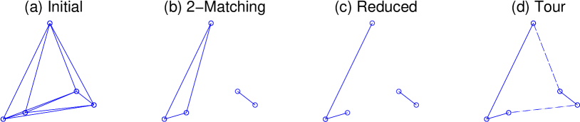
Figure 1: The steps in the 2-matching based tour algorithm

We now present an outline of the complete 2-matching tour algorithm. The steps are illustrated in Figure 1.

1. Run Algorithm 4 to get a simple 2-matching, $M_{1}$. Using the linear relaxation $\tilde{w}$ of $w$, solve for the maximum weight 2-matching, $M_{2}$. From $M_{1}$ and $M_{2}$, choose the 2-matching that has a higher reward.

2. Find all sets of subtours. (using, for example, DFS).

3. Run Algorithm 6 to select edges to remove.

4. Connect up the reduced subtours into a tour. One method to accomplish this would be by finding all the vertices that have degree of 0 or 1 and then arbitrarily connecting them up to complete the tour.

Theorem V.10.

The 2-matching tour algorithm gives a $\max\left\{\frac{2}{3(2+\kappa)},\frac{2}{3}(1-\kappa)\right\}$-approximation in $O(f(n^{3}+n)+n^{3}\log n)$ time.

Proof.

The matching is a $\max\left\{\frac{1}{2+\kappa},1-\kappa\right\}$-approximation from Theorems V.1 and V.2. Given that a tour is a special case of the maximum simple 2-matching, the maximum tour has a value less than or equal to the optimal 2-matching. Removing edges from the matching produces a subgraph that is atleast $\frac{2}{3}$ of the original value of the 2-matching (Theorem V.9). Adding more edges to complete the tour will only increase the value. Therefore, the resulting tour is within $\max\left\{\frac{2}{3(2+\kappa)},\frac{2}{3}(1-\kappa)\right\}$ of the optimal tour. Note that the bound given is relative to the optimal 2-matching and not to the optimal tour so the actual bound may be better.

The first step involves building the matching. The greedy matching takes $O(|V|^{3}(f+\log|V|))$ time and the linear relaxation approximation takes $O(|V|^{3})$ time. Finding the edges in all the components is $O(|V|+|E|)=O(|V|)$ since the number of edges in a matching is at most $|V|$. Removing the edges is $O(|V|f)$. Assuming it is easy to find the free vertices, connecting up the final graph is $O(m)=O(|V|)$ where $m$ is the number of subtours and ranges from $1$ to $\left\lfloor\frac{|V|}{3}\right\rfloor$. Therefore, the total runtime is $O(n^{3}(f+\log n)+n(2+f))=O(f(n^{3}+n)+n^{3}\log n)$. ∎

The reason for calculating the 2-matching twice is now explained. The greedy method gives a $\frac{1}{2}$-approximation in the case of a linear objective (Lemma II.8). A similar method of using a matching is used in [1] for a linear reward function. In that case, the approximation ratio achieved is $\frac{2}{3}$ of the optimal tour. The reason for this is that for a linear function, an optimal perfect matching is obtained and the bound depends only on how much is lost in removing the edges. We showed that a similar bound limiting the loss can be obtained for the submodular case; however, just using the greedy approximation for the 2-matching, we cannot guarantee as good a result since the final tour would be within $\frac{2}{3}\frac{1}{2}=\frac{1}{3}$ of the optimal. By also using the second method of finding the 2-matching, our resulting bound for the final tour in the case of a linear function improves to $\frac{2}{3}$.

Remark V.11.

For any value of $\kappa<\frac{1}{2}(\sqrt{3}-1)\approx 0.366$, using the linear relaxation method to construct a 2-matching and then converting it into a tour, gives a better bound with respect to the optimal tour than by using the greedy tour approach. $\bullet$

Remark V.12.

In our case, the $\frac{2}{3}$ loss is actually a worst case bound where all the subtours are composed of 3 edges. For a graph with a large number of vertices, the subtours will probably be larger and so $k$ may be larger than 3. This would lead to a better bound for the algorithm. $\bullet$

Remark V.13.

In removing the edges we used an algorithm to quickly find a “good” set of edges to remove but made no effort to look for the “best” set. Using a more intelligent heuristic we would get better results (of course at the cost of a longer runtime).

Also, the last step where the reduced subtours are connected into a tour can be achieved using various different techniques. As mentioned above, one possibility is to just arbitrarily connect up the components. Another method would be to use a greedy approach (so running Algorithm 3 except with an initial state). This would not change the worst case runtime given in Theorem V.10. Alternatively, if the number of subtours is found to be small, an exhaustive search going through all the possibilities could be performed. $\bullet$

VI Extension to directed graphs

The algorithms described can also be applied to directed graphs yielding approximations for the ATSP.

VI-A Greedy Tour

For the greedy tour algorithm, a slight modification needs to be made to check that the in-degree and out-degree of the vertices are less than $1$ instead of checking for the degree being less than $2$. Since the ATSP is a 3-extendible system, the approximation of the greedy algorithm changes to $\frac{1}{3+\kappa}$ instead of $\frac{1}{2+\kappa}$ as in the undirected case.

VI-B Tour using Matching

Instead of working with a 2-matching, the system can be modelled as the intersection of two partition matroids:

• Edge sets such that the indegree of each vertex $\leq 1$.

• Edge sets such that the outdegree of each vertex $\leq 1$.

This system is still 2-extendible and so the approximation for the greedy 2-matching does not change. For the second approximation, the Maximum Assignment Problem (max AP) can be solved by representing the weights in (6) as a weight matrix $\tilde{W}$ where we set $\tilde{W}_{ii}=-\infty$. The Hungarian algorithm, that has a complexity of $O(n^{3})$, can be applied to obtain an optimal solution. Therefore, the result of Theorem V.2 still applies.

The result of the greedy algorithm or the solution to the assignment problem will be a set of edges that together form a set of cycles, with the possibility of a lone vertex. Note that a “cycle” could potentially consist of just two vertices. Therefore, removing one edge from each cycle will result in a loss of at most $\frac{1}{2}$ instead of $\frac{1}{3}$. This follows directly from the analysis in Theorem V.3 but using $k=2$ instead of $k=3$. The final bound for the algorithm is therefore $\max\left\{\frac{1}{2(2+\kappa)},\frac{1}{2}(1-\kappa)\right\}$.

VII Incorporating Costs

Often times, optimization algorithms have to deal with multiple objectives. In our case, we can consider the tradeoff between the reward of a set and its associated cost. A number of algorithms presented in literature look at attempting to maximize the benefit given a “budget” or a bound on the cost, i.e. find a tour T such that

$$T\in\operatorname*{argmax}_{S\in\mathcal{H}}w(S)\text{ s.t. }c(S)\leq k.$$

This involves maximizing a monotone non-decreasing submodular function over a knapsack constraint as well as an independence system constraint.

We will work with a different form of the objective function defined by a weighted combination of the reward and cost. For a given value of $\beta\in[0,1]$, solve

$$T \in\operatorname*{argmax}_{S\in\mathcal{H}}f(S)$$ (7)

$$f(S,\beta) =(1-\beta)w(S)-\beta c(S),$$ (8)

where the combined objective is a non-monotone possibly negative submodular function. An advantage of having this form for the objective is that the “cost trade-off” is being incorporated directly into the value being optimized. Since the cost function is modular, maximizing the negative of the cost is equivalent to minimizing the cost. So the combined objective tries to maximise the reward and minimize the cost at the same time.

The parameter $\beta$ is used as a weighting mechanism. The case of $\beta=0$ corresponds to ignoring costs and that of $\beta=1$ corresponds to ignoring rewards and just minimizing the cost (this would just be the traditional TSP).

One minor issue with the proposed function is that the rewards and costs may have different relative magnitudes. This might mean that $\beta$ is biased to either 0 or 1. Normalizing the values of $w$ and $c$ will help bring both the values down to a similar scale. This gives the advantage of being able to use $\beta$ as an unbiased tuning parameter.

Therefore, the final definition of the objective function is

$$f(S)=\frac{1-\beta}{M_{w}}w(S)-\frac{\beta}{M_{c}}c(S)$$ (9)

where $M_{c}=\max_{S}{c(S)}$ and $M_{w}=\max_{S}{w(S)}$. The exact values of $M_{c}$ and $M_{w}$ may be hard to calculate and so could be approximated.

To address the issue of the function being non-monotone and negative, consider the alternative modified cost function

$$c^{\prime}(S)=|S|M-c(S),\quad M=\max_{e\in E}c(e).$$

This gives the following form for the objective function,

$$f^{\prime}(S,\beta) =(1-\beta)w(S)+\beta c^{\prime}(S)$$ (10)

$$=(1-\beta)w(S)+\beta(|S|M-c(S)),$$

$$=f(S,\beta)+\beta|S|M,$$

which is a monotone non-decreasing non-negative submodular function. This has the advantage of offering known approximation bounds. The costs have in a sense been “inverted” and so maximizing $c^{\prime}$ still corresponds to minimizing the cost $c$.

Remark VII.1.

Instead of using $|S|M$ as the offset, we could use the sum of the $|S|$ largest costs in $E$. This would not improve the worst case bound but may help to improve results in practice. $\bullet$

Lemma VII.2.

For any two sets $S_{1}$ and $S_{2}$, if $f^{\prime}(S_{1})\geq\alpha f^{\prime}(S_{2})$ then $f(S_{1})\geq\alpha f(S_{2})+M(\alpha|S_{2}|-|S_{1}|)$

Proof.

$$f^{\prime}(S_{1})\geq\alpha f^{\prime}(S_{2})$$

$$\implies f(S_{1})+|S_{1}|M\geq\alpha(f(S_{2})+|S_{2}|M)$$

$$\implies f(S_{1})\geq\alpha f(S_{2})+M(\alpha|S_{2}|-|S_{1}|)$$

∎

Remark VII.3.

As a special case, if $|S_{1}|=|S_{2}|$, then $f(S_{1})>f(S_{2})$ if and only if $f^{\prime}(S_{1})>f^{\prime}(S_{2})$. Therefore, it can be deduced that over all sets of the same size, the one that maximizes (8) is the same one that maximizes (10). $\bullet$

Theorem VII.4.

Let $G_{1}$ be the greedy solution obtained maximizing (8) and $G_{2}$ be the greedy solution maximizing (10). Then $G_{1}=G_{2}$.

Proof.

At each iteration $i$ of the greedy algorithm, we are finding the element that will give the maximum value for a set of size $i+1$. Since comparison is being done between sets of the same size, the same element will be chosen at each iteration. ∎

Theorem VII.5.

Consider a function $f=f_{1}-f_{2}$, where $f_{1}$ is submodular and $f_{2}$ is modular, and a $p$-system $(E,{\cal F})$. An $\alpha$-approximation to the problem $\max_{S\in{\cal F}}f^{\prime}(S)$, where $f^{\prime}(S)=f(S)+|S|M,M=\max_{e\in E}f_{2}(e)$, corresponds to an approximation of $\alpha OPT-\big{(}1+\alpha-2\frac{\alpha}{p}\big{)}Mn$, for the problem $\max_{S\in{\cal F}}f(S)$, where $n$ is the size of the maximum cardinality basis.

Proof.

Let $S$ be the solution obtained by a $\alpha$-approximation algorithm to $f^{\prime}$. Let $T$ be the optimal solution using $f^{\prime}$. Let $Z$ be the optimal solution using $f$. Note the following inequality:

$$|A|\leq|B|p\implies\alpha|B|-|A|\geq|B|(\alpha-p)\geq|A|(\frac{\alpha}{p}-1).$$

By using the property of $p$-systems that for any two bases $A$ and $B$,

$$\frac{|A|}{|B|}\leq p,$$

and by Lemma VII.2, we have

$$f^{\prime}(S)\geq\alpha f^{\prime}(T)\implies f(S)\geq\alpha f(T)+M\left(\alpha|T|-|S|\right).$$

So,

$$f(S) \geq\alpha f(T)-M|T|\left(p-\alpha\right)$$

$$\geq\alpha f(T)-M|S|\left(1-\frac{\alpha}{p}\right)$$

$$\geq\alpha f(T)-Mn\left(1-\frac{\alpha}{p}\right).$$

Also,

$$f^{\prime}(T)\geq f^{\prime}(Z)\implies f(T)\geq f(Z)-M|T|\left(1-\frac{1}{p}\right).$$

Substituting,

$$f(S) \geq\alpha f(Z)-\alpha M|T|\left(1-\frac{1}{p}\right)-Mn\left(1-\frac{\alpha}{p}\right)$$

$$\geq\alpha f(Z)-Mn\left(1+\frac{p-2}{p}\alpha\right).$$

∎

Remark VII.6.

In the special case of a 1-system (this includes matroids), or more generally any problem where the output to the algorithm will always be the same size, we have $|S|=|T|=|Z|$ and also $T=Z$ following from Remark VII.3. This means that an algorithm that gives a relative error of $\alpha$ when using $f^{\prime}$ as the objective will give a normalized relative error of $\alpha$ when using $f$ as the objective (i.e. $f(S)\geq\alpha{\rm OPT}+(1-\alpha){\rm WORST}$). $\bullet$

Corollary VII.7.

The problem $\max_{S\in{\cal F}}f(S)$ can be approximated to $(p+1)^{-1}OPT+(1+\epsilon)WORST$ (where $\epsilon\in[-\frac{1}{2},1)$ is a function of $p$) using a greedy algorithm.

Proof.

Let $f^{\prime}(S)=f(S)+|S|M,M=\max_{e\in E}f_{2}(e)$ and run the greedy algorithm to obtain the set $T_{G}$. Let Let $T$ and $Z$ be defined as above. Since $f^{\prime}$ is a non-negative monotone function,

$$f^{\prime}(T_{G})\geq\frac{1}{p+1}f^{\prime}(T).$$

So applying Theorem VII.5,

$$f(T_{G}) \geq\frac{1}{p+1}f(Z)-Mn\left(1+\frac{p-2}{p(p+1)}\right)$$

∎

VII-A Performance Bounds with Costs

Using the proposed modification, new bounds can be derived for the algorithms discussed in this paper. One thing to note is that in the case of the tour, all tours will be the same length that is $|V|$, even though the tour is not a 1-system. Therefore, we can apply Lemma VII.2 directly.

Theorem VII.8 (Greedy tour with edge costs).

Using (8) as the objective, Algorithm 3 outputs a tour that has a value at least $\frac{1}{3}OPT-\frac{2}{3}\beta M|V|$ where $M$ is the maximum cost of any edge.

Theorem VII.9 (Tour via 2-matching with edge costs).

Using (8) as the objective, the tour based on a matching algorithm outputs a tour that has a value at least $\frac{2}{9}OPT-\frac{7}{9}\beta M|V|$ where $M$ is the maximum cost of any edge.

The bounds given in these theorems are not the best that can be obtained. For the case when $\beta$ is small, the submodular reward is weighted higher and the bound is closer to that of maximizing a submodular function. On the other hand, for the case of large $\beta$ (specifically when $\beta=1$), the problem is just the traditional minimum cost TSP. In [18] an approximation of $\frac{1}{2}(OPT+WORST)$ was given for finding a minimum TSP using a greedy approach which is better than the $\frac{1}{3}OPT+\frac{2}{3}WORST$ that we calculate for the greedy tour with costs. In addition, simple fast methods also exist to find the minimum cost tour in a graph using other approaches. Therefore, if the costs are to be given a higher weight, the analysis given here is not very informative of the resulting solution.

VIII Simulations

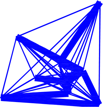
(a) Example graph.

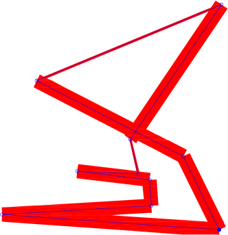
(b) Greedy solution.

Figure 2: A ten vertex graph and example solution.

In order to empirically compare our algorithms, we have run simulations for a function that represents coverage of an environment. A complete graph is generated by uniformly placing vertices over a rectangular region. Each edge in the graph is associated with a rectangle and each rectangle is assigned a width to represent different amounts of coverage.

An example of a ten vertex graph is given in Figure 2a. Here we see the complete graph as well as a representation of the value of each edge given by the area of the rectangle the edge corresponds to. The majority of edges have a low weight with a few having a much larger value. Running the greedy tour algorithm, we get the tour given in Figure 2b.

The simulations were performed on a quad-core machine with a 3.10 GHz CPU and 6GB RAM. To decrease total runtime, three instances of problems were run in parallel on different Matlab^® sessions.

VIII-A Algorithm Comparison

Next we compare the performance of the algorithms given in this paper. Each algorithm was run on randomly generated graphs for a fixed number of vertices. The resulting value of the objective function was recorded and averaged over all instances. The algorithms compared are:

• GreedyTour (GT): The greedy algorithm for constructing a tour.

• RandomTour (RT): Edges are considered in a random order. An edge is selected to be part of the tour as long as the degree constraints will be satisfied and no subtour will be created.

• For the 2-matching based algorithm, three possibilities are considered. All three start off by greedily constructing a 2-matching.

  • GreedyMatching (GM): Remove from each subtour the element that will result in the least loss to the total value. Greedily connect up the complete tour.

  • GreedyMatching2 (GM2): Use Algorithm 6 to reduce the matching. Greedily connect up the complete tour.

  • GreedyMatching3 (GM3): Use Algorithm 6 to reduce the matching. Arbitrarily connect up the complete tour.

The vertices were distributed randomly over a 100x100 region. For the first simulation, the edge thickness was assigned a value of 7 with probability $\frac{2}{\sqrt{|V|}}$, or 1 otherwise. This way, $O(|V|)$ of the edges had a high reward. A total of 30 different instances of the problem were solved by all the algorithms for 5 different graph sizes. For the second simulation, the set up was the same except the edges thickness were distributed uniformly over $[0,7]$ and a total of 40 instances were averaged.

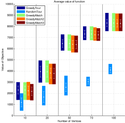
	GT	RT	GM	GM2	GM3
10	27 (3)	0 (0)	25 (1)	16 (1)	2 (0)
20	23 (8)	0 (0)	21 (5)	8 (0)	1 (0)
50	26 (16)	0 (0)	14 (4)	5 (0)	0 (0)
70	27 (18)	0 (0)	12 (3)	3 (0)	1 (0)
100	27 (16)	0 (0)	14 (3)	2 (0)	1 (0)

Figure 3: (Top) The bars give the range of results. The white markers inside the bars show the mean and standard deviation. (Bottom) Number of wins for each algorithm. Wins include ties (unique wins specified in parens).

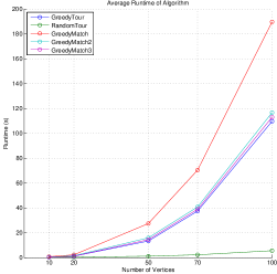
	GT	RT	GM	GM2	GM3
10	0.2	0	0.4	0.3	0.2
20	0.8	0.1	2.2	1.4	1.1
50	13.3	0.8	27.1	15.9	14.4
70	37.4	2.2	70.4	40.7	39.0
100	109.7	5.4	189.9	116.5	113.1

Figure 4: Average runtime (seconds) of algorithms.

Average runtimes of each algorithm are shown in Figure 4.

The results for the first setup are shown in Figure 3 The table gives a count of the number of times each algorithm had the largest value. Average runtimes of each algorithm are shown in Figure 4. For the second setup, the solution values and number of wins are given in Figure 5.

The RT algorithm performs poorly in each case. This is expected as no effort is put into finding good edges. For the first setup, most of the edges have a low reward and so the rewards of any random set of edges will be biased towards a small value. In the second setup, since the distribution is uniform, the expected value of the tour increases though getting close to the “best” tour is still not likely.

Both GT and GM perform similarly well on average (note that the number of ties is high especially for smaller graph sizes) though GM takes a lot longer to run. This can be explained due to the extra oracle calls required to determine which edge to remove from each subtour (a total of $|V|$ extra oracle calls).

Both GM2 and GM3 are slightly behind GM in terms of the final value. This makes sense since in GM more effort is put into finding a good reduction of the 2-matching whereas in GM2 only an attempt to find a good set of edges to remove is made. Between GM2 and GM3, the solution values are very close though GM2 runs slightly slower than GM3. The only difference between the two techniques is that the joining of the reduced subtours is performed randomly for GM3. This requires no oracle calls leading to a faster runtime. In this particular set up, the number of subtours was $o(|V|)$ so very few calculations were needed to construct the final tour from the reduced subtours. It is however possible for the number of subtours to be $O(|V|)$ and in those cases GM2 would be much slower as the problem size would not be significantly reduced by first coming up with a 2-matching.

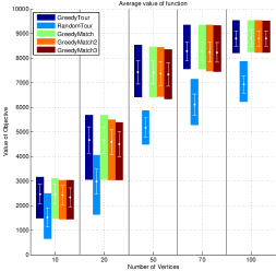
	GT	RT	GM	GM2	GM3
10	35 (10)	0 (0)	28 (3)	22 (0)	4 (0)
20	31 (8)	0 (0)	32 (9)	11 (0)	0 (0)
50	33 (13)	0 (0)	25 (5)	12 (2)	1 (0)
70	29 (10)	0 (0)	29 (10)	8 (1)	4 (0)
100	35 (5)	0 (0)	35 (5)	17 (0)	12 (0)

Figure 5: (Top) The bars give the range of results. The white markers inside the bars show the mean and standard deviation. (Bottom) Number of wins for each algorithm. Wins include ties (unique wins specified in parens).

VIII-B Dependence on Curvature

To illustrate how the results of the 2-matching based algorithm changes with curvature, the values of the greedy matching and the linear approximation are now compared. The submodular function is modified to be

$$f_{new}(S)=f(S)+\sum_{e\in S}length(e).$$

Since $f(S)$ is the total area, its value depends on the thickness of the edges. For a small thickness, the overlaps in the area between different edges will be small and so the function will be more linear. Therefore, there is a positive correlation between the edge thickness and the curvature of the function.

The experiment is performed on a ten vertex graph. The two 2-matching approximations are compared and the results are shown in Figure 6. For a second test, the GreedyTour and the 2-matching algorithm are compared and the average for 20 different ten vertex graphs is shown in Figure 7. In the figure, the “LGmatching” algorithm creates a greedy 2-matching as well as the linear approximation and takes the best of the two. The best edge from each subtour is removed and the tour is then constructed greedily. The “Lmatching” algorithm runs only the linear approximation to find the 2-matching. Figure 8 shows how the curvature changes with edge thickness.

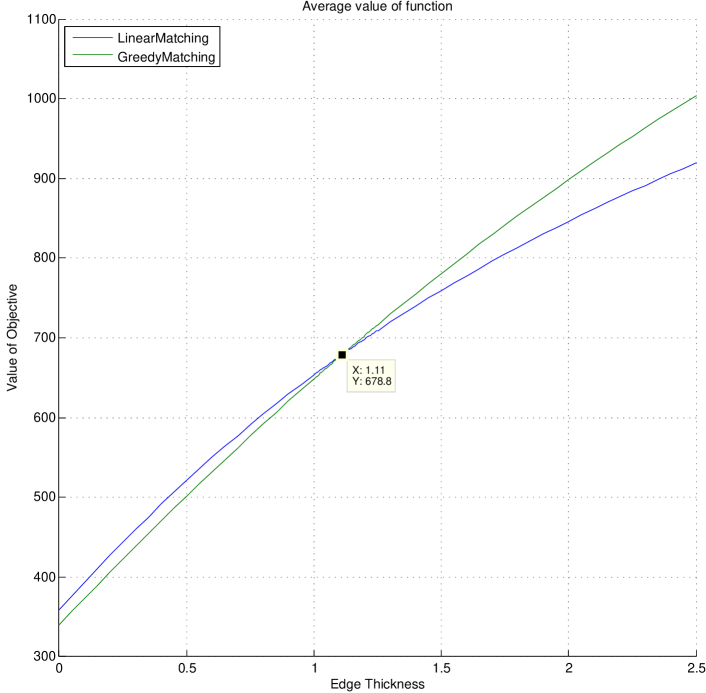
Figure 6: Curvature comparison of 2-matching algorithms

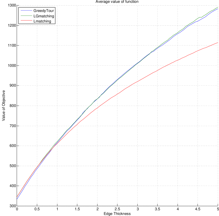
Figure 7: Curvature comparison of final tour

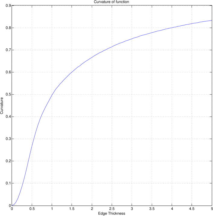
Figure 8: Curvature as a function of edge thickness

From Figure 6, we can see that for the case where the function is completely linear (thickness is 0), the linear approximation does better (since it is actually finding the optimal). The greedy matching starts to perform better at a curvature of around 0.53. Looking at the results for the value of the actual tour (Figure 7), we can see that at low values of curvature the linear approximation is being used to create the tour. Eventually, greedily constructing the 2-matching becomes more rewarding and so the linear approximation is disregarded. Generally, over all the values of curvature tested, the matching algorithm performs close to or better that the greedy tour algorithm.

IX Conclusions and Future Directions

In this paper, we extended the max-TSP problem to submodular rewards. We presented two algorithms; a greedy algorithm which achieves a $\frac{1}{2+\kappa}$ approximation, and a matching-based algorithm, which achieves a $\max\{\frac{2}{3(2+\kappa)},\frac{2}{3}(1-\kappa)\}$ approximation (where $\kappa$ is the curvature of the function). Both algorithms have a complexity of $O(|V|^{3})$ in terms of number of oracle calls. We extended these results to directed graphs and presented simulation results to empirically compare their performance as well as evaluating the dependence on curvature.

There are several directions for future work. First, we would like to determine the tightness of the bounds that were presented. The class of submodular functions is very broad and so adding further restrictions may help give a better idea of how the bounds change for specific situations. Another direction of research would be considering extending other algorithms. The strategies presented in this paper are extensions of simple algorithms that are used to obtain approximations for the traditional TSP. There are many other simple strategies that could also be extended such as best neighbour or insertion heuristics. One other possible extension would be to consider the case where multiple tours are needed (such as with multiple patrolling robots).

References

- [1] M. L. Fisher, G. L. Nemhauser, and L. A. Wolsey, “An analysis of approximations for finding a maximum weight hamiltonian circuit,” Operations Research, vol. 27, no. 4, pp. pp. 799–809, 1979.
- [2] R. Hassin and S. Rubinstein, “Better approximations for max TSP,” Information Processing Letters, vol. 75, pp. 181–186, 1998.
- [3] C. Guestrin, A. Krause, and A. Singh, “Near-optimal sensor placements in Gaussian processes,” in Int. Conf. on Machine Learning, Bonn, Germany, Aug. 2005.
- [4] D. Golovin and A. Krause, “Adaptive submodularity: Theory and applications in active learning and stochastic optimization,” Journal of Artificial Intelligence Research, vol. 42, pp. 427–486, 2011.
- [5] P. R. Goundan and A. S. Schulz, “Revisiting the greedy approach to submodular set function maximization,” 2007, Working Paper, Massachusetts Institute of Technology.
- [6] A. Singh, A. Krause, C. Guestrin, and W. Kaiser, “Efficient informative sensing using multiple robots,” Journal of Artificial Intelligence Research, vol. 34, pp. 707–755, 2009.
- [7] A. Schrijver, “A combinatorial algorithm minimizing submodular functions in strongly polynomial time,” Journal of Combinatorial Theory, Series B, vol. 80, no. 2, pp. 346 – 355, 2000.
- [8] S. Iwata, L. Fleischer, and S. Fujishige, “A combinatorial strongly polynomial algorithm for minimizing submodular functions,” J. ACM, vol. 48, no. 4, pp. 761–777, Jul. 2001.
- [9] G. L. Nemhauser, L. A. Wolsey, and M. L. Fisher, “An analysis of approximations for maximizing submodular set functions - I,” Mathematical Programming, vol. 14, pp. 265–294, 1978.
- [10] G. Calinescu, C. Chekuri, M. Pál, and J. Vondrák, “Maximizing a monotone submodular function subject to a matroid constraint,” SIAM Journal on Computing, vol. 40, no. 6, pp. 1740–1766, 2011.
- [11] M. L. Fisher, G. L. Nemhauser, and L. A. Wolsey, “An analysis of approximations for maximizing submodular set functions - II,” in Polyhedral Combinatorics, ser. Mathematical Programming Studies, 1978, vol. 8, pp. 73–87.
- [12] J. Ward, “A (k+3)/2-approximation algorithm for monotone submodular k-set packing and general k-exchange systems,” in 29th International Symposium on Theoretical Aspects of Computer Science, vol. 14, Dagstuhl, Germany, 2012, pp. 42–53.
- [13] M. Conforti and G. Cornuejols, “Submodular set functions, matroids and the greedy algorithm: Tight worst-case bounds and some generalizations of the rado-edmonds theorem,” Discrete Applied Mathematics, vol. 7, no. 3, pp. 251 – 274, 1984.
- [14] B. Korte and J. Vygen, Combinatorial Optimization: Theory and Algorithms, 4th ed., ser. Algorithmics and Combinatorics. Springer, 2007, vol. 21.
- [15] M. Minoux, “Accelerated greedy algorithms for maximizing submodular set functions,” in Optimization Techniques, ser. Lecture Notes in Control and Information Sciences, J. Stoer, Ed. Springer Berlin / Heidelberg, 1978, vol. 7, pp. 234–243.
- [16] U. Feige, “A threshold of ln n for approximating set cover,” J. ACM, vol. 45, no. 4, pp. 634–652, Jul. 1998.
- [17] J. Mestre, “Greedy in approximation algorithms,” in Algorithms – ESA 2006, Y. Azar and T. Erlebach, Eds. Springer Berlin / Heidelberg, 2006, vol. 4168, pp. 528–539.
- [18] T. A. Jenkyns, “The greedy travelling salesman’s problem,” Networks, vol. 9, no. 4, pp. 363–373, 1979.
- [19] T. H. Cormen, C. E. Leiserson, R. L. Rivest, and C. Stein, Introduction to Algorithms, 2nd ed. MIT Press, 2001.