The classification of two-loop integrand basis in pure four-dimension

Abstract:

In this paper, we have made the attempt to classify the integrand basis of all two-loop diagrams in pure four-dimensional space-time. The first step of our classification is to determine all different topologies of two-loop diagrams, i.e., the structure of denominators. The second step is to determine the set of independent numerators for each topology using Gröbner basis method. For the second step, varieties defined by putting all propagators on-shell has played an important role. We discuss the structures of varieties and how they split to various irreducible branches under specific kinematic configurations of external momenta. The structures of varieties are crucial to determine coefficients of integrand basis in reduction both numerically or analytically.

1 Introduction

In the past few years we have seen tremendous progresses for one-loop diagram computations using Passrino-Veltman(PV) reduction method [3]. The newly developed reduction methods can be sorted into two categories: (a) the reduction performed at the integral level, such as the unitarity cut method [4, 5, 6, 7, 8] and generalized unitarity cut method[9, 10]; (b) the reduction performed at the integrand level, which was initiated by Ossola-Papadopoulos-Pittau(OPP) in [11] and further generalized in [12, 13, 14, 15, 16, 17]. Comparing methods of these two categories, methods in the first one focus only on coefficients having nonzero final contributions while methods in the second one must also include spurious coefficients. Although more coefficients must be calculated, methods in the second category are still very useful because all manipulations are performed purely algebraically at the integrand level, thus they can be easily programmed.

Encouraged by successful computations at one-loop level, it is natural to generalize these methods to higher loops, partially because of our theoretical curiosity and partially because of the precise prediction for modern collide experiments. However, the generalization is not so trivial. The first difficulty is that in general we do not know much about the basis for multi-loop amplitudes. In fact, now it is clear that we should distinguish the integral basis and the integrand basis. Unlike the one-loop amplitude, the number of integrand basis is much larger than the number of integral basis for multi-loop amplitudes. Thus it is highly desirable to reduce integrand basis to integral basis further. One standard method of doing so is the Integrate-by-Part (IBP) method[18]. The IBP can be carried out in a reasonable short time if the amplitude involves only a few external particles, but it becomes unpractical with time consuming when the number of external particles increases. The second difficulty is how to extract coefficients of basis. For one-loop amplitudes, finding coefficients is separated from finding basis, while the frequently-used IBP reduction method combines these two tasks together at the same time.

These computation difficulties for multi-loop amplitudes have been addressed in the past few years by several groups [19, 20, 21, 22, 23, 24, 25, 26, 27, 28, 29]. The main focus of study is the reduction at integrand level, which includes finding integrand basis and matching their coefficients. The step towards this direction was first taken in [19], where four-dimensional constructive algorithm for integrand has been applied to two-loop planar and non-planar contributions of four and five-point Maximal-Helicity-Violating(MHV) amplitudes in $\mathcal{N}=4$ Super-Yang-Mills theory. Using constraints from Gram matrix, similar determinant of monomials of numerators was achieved in [20]. Besides reduction at the integrand level, reduction at the integral level is discussed in [21, 22, 23, 24, 25], where in order to determine the physical contour for integral basis, the variety defined by setting all propagators on-shell has been carefully analyzed.

Among these new developments, the application of computational algebraic geometry method to multi-loop amplitude calculations is very intriguing [27, 28], where the Gröbner basis plays a central role. It is quite easy to determine integrand basis by Gröbner basis method, although different sets of integrand basis can be obtained with different orderings in polynomial division. Besides the integrand basis, their coefficients can also be determined by the same method. The knowledge of variety, including its branch structure and intersection pattern of branches, is very important in the application of this method. This method has been tested by several examples in at two and three-loops [27, 29]. Encouraged by the success, in this paper we will use algebraic geometry method to systematically study all possible topologies of two-loop diagrams in pure four-dimension for any external momentum configurations, not only restrict to double-box or penta-triangle studied in various references.

The paper is organized as follows. In section 2 we classify all possible topologies for two-loop diagrams. In section 3 the one-loop topologies are re-examined using algebraic geometry method. Ideas from the reexamination will be used to analyze two-loop topologies. In section 4, as a warm-up, we present results of some trivial two-loop topologies. In section 5, a careful analysis of planar penta-triangle topology has been given, while in section 6, we give a detailed study of non-planar crossed double-triangle topology. In section 7, we summarize results of all remaining topologies. In the last section, conclusions and discussions are given. In appendix, we introduce some mathematical facts that can be used to study the branch structure of variety.

2 An overview of general two-loop topologies

In this section, we give an overview of general two-loop topologies. Much of the results are scattered in literatures, and we assemble them here to make the paper self-contained.

2.1 The two-loop topology

Since two-loop diagrams can always be reduced to one-loop diagrams by cutting an inner propagator, we can inversely reconstruct two-loop ones by sewing two external legs of one-loop diagrams. The topology of one-loop diagrams is very simple: we just attach various tree structures along the loop at some vertices $V_{i}$ (see Figure 1 ).

Figure 1: The general topology of one-loop diagrams where various tree structures are attached along the loop at some vertices.

From one-loop topology we can reconstruct two-loop topology by connecting two external legs, and there are several ways of doing so, which give different two-loop topologies:

• (A) If the two to-be-connected external legs are attached to the same tree structure, we will get two-loop topology as drawn in Figure 2. Explicit illustration shows that there are two kinds of connections. In the first kind (A1), two one-loop sub-topologies do not share the same vertex while in the second kind (A2), they do share a common vertex.

  

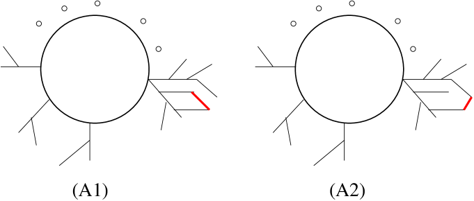
  Figure 2: The two-loop topology generated from one-loop topology by connecting two external legs attached to the same tree structure. The connection has been denoted by red color thick line. In connection (A1), two one-loop sub-topologies do not share the same vertex while in connection (A2), they do share a common vertex.

• (B) If the two to-be-connected external legs are attached to two nearby vertices along the loop, we will get two-loop topology as drawn in (B) of Figure 3. All two-loop planar topologies can be generated from this type.

  

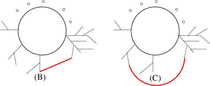
  Figure 3: The two-loop topologies of case (B) and case (C) obtained by connecting two external legs attached to two different tree structures. For case (B), two tree structures are adjacent while for case (C), not adjacent.

• (C) If the two to-be-connected external legs are attached to two non-nearby tree structures along the loop, we will get two-loop topology as drawn in (C) of Figure 3. All two-loop non-planar topologies can be generated from this type.

2.2 Classification of denominators of two-loop basis

Having understood the general two-loop topologies, the next step is to classify the basis used to expand any two-loop amplitudes. This is similar to the classification of scalar basis for one-loop diagrams, which includes box, triangle, bubble and tadpole. However, it is necessary to distinguish the integrand basis and the integral basis. The integrand basis is that used by OPP method to expand expressions coming from Feynman diagrams at integrand level. However, after carrying out the integrations, some elements of integrand basis will vanish, while others may have nontrivial linear relations. After excluded these redundancies from integrand basis we obtain the integral basis. The integral basis is also called the master integrals(MIs). The number of integral basis is much smaller than the number of integrand basis, since after integration. The difference between these two kinds of basis can be easily seen in the one-loop box topology: there is only one master integral ${1\over D_{1}D_{2}D_{3}D_{4}}$, but there are two integrand basis ${1\over D_{1}D_{2}D_{3}D_{4}}$ and ${\epsilon(\ell,K_{1},K_{2},K_{3})\over D_{1}D_{2}D_{3}D_{4}}$. Numerator of $\epsilon\cdot\ell$ with odd power will vanish after integration because of parity.

To find the integrand and integral basis, we can use the procedure called PV-reduction. Among manipulations on expressions coming from Feynman diagrams, some are done at the integrand level, such as rewriting $2K_{1}\cdot\ell=-(\ell-K_{1})^{2}+\ell^{2}+K_{1}^{2}$, while some manipulations are carried out using properties of integral, such as IBP method. Pure algebraic manipulations at the integrand level will produce the integrand basis, while combining with operations such as IBP, will reduce integrand basis further to integral basis. Above reduction has been discussed in many references, for example, [25] for details and reference.

For two-loop diagrams, denominators of expressions coming from Feynman diagrams can always be written as products of three kinds of propagators

$$\mathcal{D} = D\widetilde{D}\widehat{D}~{},~{}~{}~{}$$ (1)

where

$$D = \ell_{1}^{2}(\ell_{1}-K_{a,1})^{2}(\ell_{1}-K_{a,2})^{2}...(\ell_{1}-K_{a,n_{1}-1})^{2}~{},~{}~{}~{}$$

$$\widetilde{D} = \ell_{2}^{2}(\ell_{2}-K_{b,1})^{2}(\ell_{2}-K_{b,2})^{2}...(\ell_{2}-K_{b,n_{2}-1})^{2}~{},~{}~{}~{}$$

$$\widehat{D} = (\ell_{1}+\ell_{2}+K_{c,1})^{2}...(\ell_{1}+\ell_{2}+K_{c,n_{3}})^{2}~{}.~{}~{}~{}$$ (2)

Here $n_{1}$, $n_{2}$ are numbers of propagators containing only $\ell_{1}$ or $\ell_{2}$, while $n_{3}$ is the number of propagators containing both $\ell_{1},\ell_{2}$. By the freedom of relabeling $\ell_{1},\ell_{2}$, we can always restrict $n_{i}$ with condition

$$n_{1}\geq n_{2}\geq n_{3}~{}.~{}~{}~{}$$ (3)

The up-bound of $n_{1},n_{2},n_{3}$ and their summation depend on the space-time dimension. For example, if we consider physics in $(4-2\epsilon)$-dimension, we would have

$$n_{1},~{}n_{2},~{}n_{3}\leq 5~{},~{}~{}~{}n_{1}+n_{2}+n_{3}\leq 11~{}.~{}~{}$$ (4)

But if we constrain to pure four-dimension, the condition becomes

$$n_{1},~{}n_{2},~{}n_{3}~{}\leq 4~{},~{}~{}~{}n_{1}+n_{2}+n_{3}\leq 8~{}.~{}~{}~{}$$ (5)

By combining conditions (3) and (5) for 4-dimension case (or (3) and (4) for $(4-2\epsilon)$-dimension case), we can classify denominators of integrand and integral. For $(4-2\epsilon)$-dimension, conditions (3) and (4) constrain $n_{3}\leq 3$. Thus if we arrange all possible solutions of $(n_{1},n_{2},n_{3})$ by value of $n_{3}$, we have following 4 groups of solutions

$$n_{3}=3: (5,3,3),(4,4,3),(4,3,3),(3,3,3)~{};~{}~{}~{}$$

$$n_{3}=2: (5,4,2),(5,3,2),(4,4,2),(5,2,2),(4,3,2),(4,2,2),(3,3,2),(3,2,2),(2,2,2)~{};~{}~{}~{}$$

$$n_{3}=1: (5,5,1),(5,4,1),(5,3,1),(4,4,1),(5,2,1),(4,3,1),(5,1,1),(4,2,1),$$

$$(3,3,1),(4,1,1),(3,2,1),(3,1,1),(2,2,1),(2,1,1),(1,1,1)~{};~{}~{}~{}$$

$$n_{3}=0: (5,5,0),(5,4,0),(5,3,0),(4,4,0),(5,2,0),(4,3,0),(5,1,0),(4,2,0),(3,3,0),$$ (6)

$$(4,1,0),(3,2,0),(3,1,0),(2,2,0),(2,1,0),(1,1,0)~{}.~{}~{}~{}$$

For pure four-dimension, the number of solutions decreases a lot, since now we have $n_{3}\leq 2$. The possible solutions of $(n_{1},n_{2},n_{3})$ for (3) and (5) are listed into 3 groups:

$$n_{3}=2: (4,2,2),(3,3,2),(3,2,2),(2,2,2)~{};~{}~{}$$ (7)

$$n_{3}=1: (4,3,1),(4,2,1),(3,3,1),(4,1,1),(3,2,1),(3,1,1),(2,2,1),(2,1,1),(1,1,1)~{};~{}~{}~{}$$

$$n_{3}=0: (4,4,0),(4,3,0),(4,2,0),(3,3,0),(4,1,0),(3,2,0),(3,1,0),(2,2,0),(2,1,0),(1,1,0)~{}.~{}~{}~{}$$

Solutions with $n_{3}=0$ contain two-loop topologies coming from sewing two one-loop topologies at a single vertex as shown in Figure 4 , while solutions with $n_{3}=1$ contain planar two-loop topologies with one common propagator as shown in Figure 5. All two-loop non-planar topologies are included in solutions $n_{3}=2$ as shown in Figure 6.

While two-loop topologies of basis have been classified by $(n_{1},n_{2},n_{3})$, to get the integrand or integral basis, we still need to determine corresponding numerators. For two-loop the so called ”scalar basis” is not enough to expand all amplitudes, we also need terms with numerators containing Lorentz invariant scalar product having internal momenta. The distinction between integrand and integral basis becomes important when discussing the classification of numerators. In this paper, we will focus only on the integrand basis in pure four-dimension.

3 The integrand basis of one-loop diagrams in pure four-dimension

As a warm-up, we take the one-loop integrand basis as a simple example to demonstrate various ideas that we will meet in later part of this paper. All results in this section are known in other references such as [11, 27, 28], however, we recall them here since these results are also related to two-loop integrand basis with $n_{3}=0$.

In pure four-dimension, since each external or internal momentum has four components, we need four independent momenta to expand all kinematics. One construction of momentum basis is to take two arbitrary independent momenta $K_{1},K_{2}$ and construct following four null momenta $e_{i}$, $i=1,2,3,4$ (assuming $(K_{1}+K_{2})^{2}\neq 0$)

$$e_{1} = {1\over\gamma_{12}}\left(K_{1}-{K_{1}^{2}+K_{1}\cdot K_{2}-{\rm sgn}(K_{1}\cdot K_{2})|\sqrt{(K_{1}\cdot K_{2})^{2}-K_{1}^{2}K_{2}^{2}}|\over(K_{1}+K_{2})^{2}}K_{12}\right)~{},~{}~{}~{}$$

$$e_{2} = {1\over\gamma_{12}}\left(K_{2}-{K_{2}^{2}+K_{1}\cdot K_{2}-{\rm sgn}(K_{1}\cdot K_{2})|\sqrt{(K_{1}\cdot K_{2})^{2}-K_{1}^{2}K_{2}^{2}}|\over(K_{1}+K_{2})^{2}}K_{12}\right)~{},~{}~{}~{}$$

$$e_{3} = {\left\langle e_{1}|\gamma^{\mu}|e_{2}\right]\over 2i}~{},~{}~{}~{}e_{4}={\left\langle e_{2}|\gamma^{\mu}|e_{1}\right]\over 2i}~{},~{}~{}~{}$$ (8)

where $\gamma_{12}^{2}={2[(K_{1}\cdot K_{2})^{2}-K_{1}^{2}K_{2}^{2}]\over(K_{1}+K_{2})^{2}}$. This momentum basis has following property: among all inner products of $e_{i}\cdot e_{j}$, the only non-zero ones are $e_{1}\cdot e_{2}=1$ and $e_{3}\cdot e_{4}=1$. Definition (8) also makes massless limit smoothly, i.e., when $K_{1}^{2}\to 0$, $e_{1}\to K_{1}$ and when $K_{2}^{2}\to 0$, $e_{2}\to K_{2}$. Using above momentum basis, we can expand any momentum, such as

$$K_{i}=(K_{i}\cdot e_{2})e_{1}+(K_{i}\cdot e_{1})e_{2}+(K_{i}\cdot e_{4})e_{3}+(K_{i}\cdot e_{3})e_{4}~{},~{}~{}~{}$$

$$\ell=(\ell\cdot e_{2})e_{1}+(\ell\cdot e_{1})e_{2}+(\ell\cdot e_{4})e_{3}+(\ell\cdot e_{3})e_{4}\equiv x_{2}e_{1}+x_{1}e_{2}+x_{4}e_{3}+x_{3}e_{4}~{},~{}~{}~{}$$ (9)

and the Lorentz invariant scalar products are given by

$$\ell^{2} = x_{1}x_{2}+x_{3}x_{4}~{},~{}~{}~{}\ell\cdot K_{i}=\sum_{j=1}^{4}{\alpha}_{ij}x_{j}~{}.~{}~{}~{}$$ (10)

The importance of above expansions (9) and (10) is that any integrand can be written as a rational function ${f(x_{1},x_{2},x_{3},x_{4})\over\prod_{t}D_{t}(x_{1},x_{2},x_{3},x_{4})}$, and the PV-reduction procedure is equivalent to finding following expansion of numerator

$$f(x_{i})=\sum_{t}c_{t}(x_{i})D_{t}(x_{i})+r(x_{i})~{},~{}~{}$$ (11)

where the remaining polynomial $r(x_{i})$ is nothing but the integrand basis we are looking for. In a more mathematical language, propagators $D_{t}$ generate an ideal $I$ in polynomial ring $k[x_{1},x_{2},x_{3},x_{4}]$, and the integrand basis is constructed by representative elements in the quotient ring $k/I$ under some physical constraints. One physical constraint is the total degree $n_{\ell}$ of loop momentum $\ell$ in numerator. For renormalizable theory, we require $n_{\ell}\leq n_{D}$ where $n_{D}$ is the number of propagators in denominator.

Having these general preparations, we will discuss explicitly various one-loop integrand basis, such as box, triangle, bubble and tadpole [11, 27, 28]. For simplicity, we will only consider massless propagators, but the massive ones can be discussed in a similar way.

3.1 One-loop box topology

For box topology, four propagators are given by

$$D_{0}=\ell^{2}~{},~{}D_{1}=(\ell-K_{1})^{2}~{},~{}D_{2}=(\ell-K_{1}-K_{2})^{2}~{},~{}D_{3}=(\ell-K_{1}-K_{2}-K_{3})^{2}~{}.~{}~{}~{}$$ (12)

Without loss of generality, we can use $K_{1},K_{2}$ to construct momentum basis and use it to expand all momenta. There are 4 variables $(x_{1},x_{2},x_{3},x_{4})$ coming from loop momentum expansion. All above propagators can be translated into following polynomials of $x_{i}$ variables

$$D_{0} = x_{1}x_{2}+x_{3}x_{4}~{},~{}D_{1}=D_{0}-2({\alpha}_{11}x_{1}+{\alpha}_{12}x_{2})+2{\alpha}_{11}{\alpha}_{12}~{},~{}~{}~{}$$

$$D_{2} = D_{0}-2({\alpha}_{21}x_{1}+{\alpha}_{22}x_{2})+2{\alpha}_{21}{\alpha}_{22}~{},~{}~{}~{}$$

$$D_{3} = D_{0}-2({\alpha}_{31}x_{1}+{\alpha}_{32}x_{2}+{\alpha}_{33}x_{3}+{\alpha}_{34}x_{4})+2{\alpha}_{31}{\alpha}_{32}+2{\alpha}_{33}{\alpha}_{34}~{},~{}~{}~{}$$ (13)

where we have used the parametrization $K_{1}+...+K_{i}\equiv\sum_{t=1}^{4}{\alpha}_{it}e_{t}$. It is easy to see that $(D_{0}-D_{1})/2={\alpha}_{11}x_{1}+{\alpha}_{12}x_{2}-{\alpha}_{11}{\alpha}_{12}$ belongs to the ideal generated by $D_{0},D_{1},D_{2},D_{3}$. However, the linearity of this equation means that in quotient ring $k[x_{1},x_{2},x_{3},x_{4}]/I$, we can always treat variable $x_{1}$ as combination ${\alpha}_{12}-{{\alpha}_{12}\over{\alpha}_{11}}x_{2}$. In other words, we can use equation $0={\alpha}_{11}x_{1}+{\alpha}_{12}x_{2}-{\alpha}_{11}{\alpha}_{12}$ to solve $x_{1}$ and eliminate variable $x_{1}$ from the quotient ring $k[x_{1},x_{2},x_{3},x_{4}]/I$. Similarly using other two linear equations $(D_{0}-D_{2}),(D_{0}-D_{3})$ we can solve variables $x_{2},x_{3}$

$${x_{1}} = \frac{{\alpha}_{12}{\alpha}_{22}({\alpha}_{11}-{\alpha}_{21})}{{\alpha}_{11}{\alpha}_{22}-{\alpha}_{12}{\alpha}_{21}}~{}~{},~{}~{}{x_{2}}=\frac{{\alpha}_{11}{\alpha}_{21}({\alpha}_{12}-{\alpha}_{22})}{{\alpha}_{12}{\alpha}_{21}-{\alpha}_{11}{\alpha}_{22}}~{},~{}~{}~{}$$

$${x_{3}} = {-{x_{4}}{\alpha}_{34}-{\alpha}_{21}{\alpha}_{32}+{\alpha}_{31}{\alpha}_{32}\over{\alpha}_{33}}+\frac{{\alpha}_{12}({\alpha}_{11}-{\alpha}_{21})({\alpha}_{21}{\alpha}_{32}-{\alpha}_{22}{\alpha}_{31})}{{\alpha}_{33}({\alpha}_{11}{\alpha}_{22}-{\alpha}_{12}{\alpha}_{21})}+{\alpha}_{34}~{}.~{}~{}~{}$$ (14)

Since $x_{1},x_{2},x_{3}$ have been solved as linear polynomial of $x_{4}$, we will call them reducible scalar products (RSP), while the remaining variable $x_{4}$, irreducible scalar products (ISP).

After substituting solution (14) into $D_{0}$ we get a quadratic polynomial of single variable $x_{4}$

$$D_{0}(x_{4})=-{{\alpha}_{34}\over{\alpha}_{33}}x_{4}^{2}+c_{1}x_{4}+c_{0}~{},~{}~{}~{}$$ (15)

where

$$c_{1} = \frac{{\alpha}_{12}{\alpha}_{21}({\alpha}_{31}({\alpha}_{32}-{\alpha}_{22})+{\alpha}_{33}{\alpha}_{34})+{\alpha}_{11}({\alpha}_{12}({\alpha}_{22}{\alpha}_{31}-{\alpha}_{21}{\alpha}_{32})+{\alpha}_{22}(({\alpha}_{21}-{\alpha}_{31}){\alpha}_{32}-{\alpha}_{33}{\alpha}_{34}))}{({\alpha}_{12}{\alpha}_{21}-{\alpha}_{11}{\alpha}_{22}){\alpha}_{33}}~{},~{}~{}~{}$$

$$c_{0} = -\frac{{\alpha}_{11}{\alpha}_{12}{\alpha}_{21}{\alpha}_{22}({\alpha}_{11}-{\alpha}_{21})({\alpha}_{12}-{\alpha}_{22})}{({\alpha}_{12}{\alpha}_{21}-{\alpha}_{11}{\alpha}_{22})^{2}}~{}.~{}~{}~{}$$ (16)

The problem of finding integrand basis for box topology is then reduced to finding representative elements in quotient ring $k[x_{4}]/\left\langle D_{0}(x_{4})\right\rangle$. Since (15) is a quadratic polynomial, the representative elements in quotient ring can take following two terms: $1$ and $x_{4}$. It is worth to notice that although in this example the dimension of quotient ring is finite, it is not true in general. In fact, if we consider the quotient ring as linear space, in general the dimension of it will be infinity, i.e., there are infinite number of representative elements. Only when some constraints are imposed we get finite number of representative elements.

There is another issue regarding to the ideal defined by (15). The quadratic polynomial is reducible, i.e., it can be factorized as product of two factors $a(x_{4}-z_{1})(x_{4}-z_{2})$ where $z_{1},z_{2}$ are two roots. This will split the solution space into two branches, which are obtained by setting either factor to zero. The variety defined by this polynomial is the union of two branches (here is just two points). Both branches are needed to analytically (or numerically) determine coefficients of two integrand basis ${1\over D_{0}D_{1},D_{2}D_{3}}$ and ${x_{4}\over D_{0}D_{1},D_{2}D_{3}}$ at the integrand level. One of the main focus of this paper is varieties determined by setting all propagators of a given topology to zero. Their branch structures as well as degeneracy for specific kinematic configurations, such as massless limit of external momenta or some attached momenta becoming zero, will be studied carefully.

3.2 One-loop triangle topology

The three propagators are given by $D_{0},D_{1},D_{2}$ as in (12), thus we can solve

$${x_{1}}=\frac{{\alpha}_{12}{\alpha}_{22}({\alpha}_{11}-{\alpha}_{21})}{{\alpha}_{11}{\alpha}_{22}-{\alpha}_{12}{\alpha}_{21}}~{},~{}{x_{2}}=\frac{{\alpha}_{11}{\alpha}_{21}({\alpha}_{22}-{\alpha}_{12})}{{\alpha}_{11}{\alpha}_{22}-{\alpha}_{12}{\alpha}_{21}}~{}.~{}~{}~{}$$ (17)

For triangle, $x_{1},x_{2}$ become RSPs, while $x_{3},x_{4}$ are left as ISPs. Putting them back to $D_{0}$ we obtain

$$D_{0}(x_{3},x_{4})=\frac{{\alpha}_{11}{\alpha}_{12}{\alpha}_{21}{\alpha}_{22}({\alpha}_{11}-{\alpha}_{21})({\alpha}_{22}-{\alpha}_{12})}{({\alpha}_{12}{\alpha}_{21}-{\alpha}_{11}{\alpha}_{22})^{2}}+{x_{3}}{x_{4}}~{}.~{}~{}~{}$$ (18)

The quotient ring is given by $k[x_{3},x_{4}]/\left\langle D_{0}(x_{3},x_{4})\right\rangle$. Its representative elements can be taken as $1,x_{3}^{n_{3}},x_{4}^{n_{4}}$ with $n_{3},n_{4}\geq 1$. Unlike the box topology, the dimension of this quotient ring will be infinity. To select finite number of representative elements from quotient ring, we constrain the power $n_{3},n_{4}$ to be no larger than three. This corresponds to the condition that the power of $\ell$ in numerator is no more than three for triangle topology. Under this constraint we get following seven representative elements $\{1,x_{3},x_{4},x_{3}^{2},x_{4}^{2},x_{3}^{3},x_{4}^{3}\}$ as given in [11].

After getting the integrand basis, we need to find their coefficients in expansion of amplitudes. For this purpose, understanding the variety defined by (18) becomes important. Assuming that the equation is given by $x_{3}x_{4}+d=0$ with $d\neq 0$, we can solve $x_{3}=-d/x_{4}$. Putting $x_{3}$ back to integrand basis we get seven monomials of $x_{4}$ only: $x_{4}^{t}$ with $t=-3,-2,-1,0,1,2,3$. Thus to find coefficients of integrand basis, we just need to substitute $x_{1},x_{2},x_{3}$ as functions of $x_{4}$ into integrand obtained by Feynman diagrams or sewing three on-shell amplitudes using unitarity cut method. Having the monomial of $x_{4}$, we can identify corresponding coefficients for a each power of $x_{4}$. For numerical analysis, we can take seven arbitrary values of $x_{4}$ to write down seven linear equations and by solving them, find the seven unknown coefficients of integrand basis.

There is a technical issue regarding to the method we just described. To guarantee that we will get exactly the form $\sum_{t=-3}^{+3}c_{t}x_{4}^{t}$, we must first subtract all contributions from box topologies. Similar manipulation should be taken when finding coefficients for bubble and tadpole at one-loop. In other words, we should subtract contributions from all other higher topologies which contain the same set of propagators in the problem.

The procedure we have just described is called parametrization of variety. For the simple example with $d\neq 0$, there is only one irreducible branch parameterized by $x_{4}$. However, with some specific kinematic configurations, above branch can split to two branches. This happens when $K_{1}^{2}=0$, so ${\alpha}_{12}=0$ or $K_{2}^{2}=0$, so $({\alpha}_{21}-{\alpha}_{11})({\alpha}_{22}-{\alpha}_{12})=0$, or $K_{3}^{2}=(K_{1}+K_{2})^{2}=0$, so ${\alpha}_{21}{\alpha}_{22}=0$. In other words, when at least one leg is massless, the definition equation of variety is reduced to $x_{3}x_{4}=0$, and we get two irreducible branches. The first branch is parameterized by setting $x_{3}=0$ with $x_{4}$ as free parameter, and the second branch, by setting $x_{4}=0$ with $x_{3}$ as free parameter. Using the parametrization of the first branch, integrand basis $x_{3}^{n}$ with $n=1,2,3$ will be zero and their coefficients can not be detected by method described in previous paragraph. It means that the first branch can only be used to find four coefficients of integrand basis $1,x_{4},x_{4}^{2},x_{4}^{3}$. Similarly, the second branch can only be used to find coefficients of integrand basis $1,x_{3},x_{3}^{2},x_{3}^{3}$. These two branches intersect at one point $x_{3}=x_{4}=0$, thus we have $4+4-1=7$, i.e., both branches are necessary to fully determine coefficients of integrand basis.

3.3 One-loop bubble topology

Because of momentum conservation there is only one external momentum. In this case, we take $K_{1}$ and another auxiliary momentum $P$ to construct the momentum basis. With two propagators $D_{0},D_{1}$ we can solve

$${x_{1}}={\alpha}_{12}\left(1-\frac{{x_{2}}}{{\alpha}_{11}}\right)~{},~{}~{}~{}$$ (19)

and there are three ISPs $(x_{2},x_{3},x_{4})$. After eliminating $x_{1}$, $D_{0}$ becomes polynomial of three ISPs

$$D_{0}(x_{2},x_{3},x_{4})={x_{2}}{\alpha}_{12}\left(1-\frac{{x_{2}}}{{\alpha}_{11}}\right)+{x_{3}}{x_{4}}~{},~{}~{}$$ (20)

which defines the variety in polynomial ring $k[x_{2},x_{3},x_{4}]$. Unlike box and triangle topologies, it is hard to find representative elements in the quotient ring

$$k[x_{2},x_{3},x_{4}]/\left\langle D_{0}(x_{2},x_{3},x_{4})\right\rangle$$

and we need a systematic way to do so. A good way is to use the Gröbner basis of ideal. Firstly we write down all possible monomials $x_{2}^{n_{2}}x_{3}^{n_{3}}x_{4}^{n_{4}}$ with $n_{2}+n_{3}+n_{4}\leq 2$ required by physical constraints. Then we divide each monomial $x_{2}^{n_{2}}x_{3}^{n_{3}}x_{4}^{n_{4}}$ by Gröbner basis and collect all monomials in the remainder. These monomials collected from the remainder times ${1\over D_{0}D_{1}}$ give the integrand basis.

A technical issue of above algorithm is the ordering of ISPs in the constructing of Gröbner basis. Different ordering gives, in general, different Gröbner basis and different sets of representative elements, although they are equivalent to each other. Once a particular ordering is chosen, we should stick to it through the whole calculation to avoid inconsistency. For instance, if the ordering is chosen as $x_{3}>x_{4}>x_{2}$ we get 9 integrand basis as

$$\left\{1,{x_{2}},{x_{2}}^{2},{x_{3}},{x_{2}}{x_{3}},{x_{3}}^{2},{x_{4}},{x_{2}}{x_{4}},{x_{4}}^{2}\right\}~{}.~{}~{}~{}$$ (21)

This integrand basis can be used to expand bubble topology. In order to get the coefficients of integrand basis analytically, we should first put $\ell=x_{2}e_{1}+x_{1}e_{2}+x_{4}e_{3}+x_{3}e_{4}$ back into integrand after subtracting all box and triangle contributions. Then we can replace $x_{1}$ by (19), and get a polynomial $A(x_{2},x_{3},x_{4})$. The next step is to divide this polynomial by Grönber basis and obtain the remainder. This algorithm, different from previous parametrization method, ensures that the remainder is nothing but the linear combination of monomials in integrand basis with coefficients we want to find.

If using the parametrization method, we can replace $x_{3}=-{\alpha}_{12}{x_{2}\over x_{4}}(1-{x_{2}\over{\alpha}_{11}})$ in the expression $A(x_{2},x_{3},x_{4})$ as well as integrand basis, and get

$$\frac{c(6){x_{2}}^{4}{\alpha}_{12}^{2}}{{x_{4}}^{2}{\alpha}_{11}^{2}}-\frac{2c(6){x_{2}}^{3}{\alpha}_{12}^{2}}{{x_{4}}^{2}{\alpha}_{11}}+\frac{c(5){x_{2}}^{3}{\alpha}_{12}}{{x_{4}}{\alpha}_{11}}+\frac{c(6){x_{2}}^{2}{\alpha}_{12}^{2}}{{x_{4}}^{2}}+\frac{c(4){x_{2}}^{2}{\alpha}_{12}}{{x_{4}}{\alpha}_{11}}-\frac{c(5){x_{2}}^{2}{\alpha}_{12}}{{x_{4}}}$$

$$-\frac{c(4){x_{2}}{\alpha}_{12}}{{x_{4}}}+c(3){x_{2}}^{2}+c(8){x_{2}}{x_{4}}+c(2){x_{2}}+c(9){x_{4}}^{2}+c(7){x_{4}}+c(1)~{}.~{}~{}~{}$$

Since we have already used the equation to reduce one variable further, remaining variables $x_{2},x_{4}$ are totally free variables. What we need to do is to compare each independent monomial $x_{4}^{a}x_{2}^{b}$ ($a,b$ could be negative integers) at both sides. The parametrization method can also be used for numerical fitting. We only need to write down enough linear equations to solve coefficients by taking sufficient numerical values $(x_{2},x_{4})$ at both sides.

Similar to triangle topology, the variety defined by (20) is irreducible for general kinematic configuration. However, when $K_{1}^{2}=0$ we have ${\alpha}_{12}=0$ by our construction, thus equation (20) is reduced to $x_{3}x_{4}=0$. In other words, the variety is degenerated to two branches: one with $x_{3}=0$ and $x_{2},x_{4}$ as free parameters, and another with $x_{4}=0$ and $x_{2},x_{3}$ as free parameters. Each branch can detect six coefficients out of nine integrand basis, while three basis $\{1,x_{2},x_{2}^{2}\}$ can be detected by both branches. Thus we have $6+6-3=9$, and both branches are necessary to find all coefficients of integrand basis analytically or numerically.

3.4 One-loop tadpole topology

In this case, we choose arbitrary two independent momenta to construct the momentum basis. Since there is only one propagator $D_{0}$, all four variables $x_{i}$, $i=1,2,3,4$ are ISPs and the variety is defined by equation

$$D_{0}=x_{1}x_{2}+x_{3}x_{4}~{}.~{}~{}~{}$$ (22)

Requiring the total dimension of monomials to be no larger than one, we get following basis

$$\{1,x_{1},x_{2},x_{3},x_{4}\}~{}.~{}~{}~{}$$ (23)

This variety is irreducible and we can parameterize it by solving $x_{1}=-{x_{3}x_{4}\over x_{2}}$. Thus after putting $x_{1}$ back to integrand after subtracted all contributions from boxes, triangles and bubbles, we can read out coefficients of one-loop tadpole integrand basis by comparing monomials of $x_{2}^{a}x_{3}^{b}x_{4}^{c}$.

4 A premiere: some trivial two-loop topologies

Starting from this section, we will discuss the integrand basis and variety of various two-loop topologies classified in (7) using the same method presented in previous section for one-loop topologies. Before we discuss non-trivial topologies, there are some topologies whose integrand basis and structure of variety are quite simple. These include two cases. The first case is all topologies of type (A), where two one-loop sub-structures share only one single vertex. The second case is all topologies having maximal number of propagators, i.e., 8 propagators for pure 4-dimensional two-loop diagrams.

Figure 4: The type (A) contains $10$ topologies with $n_{3}=0$. Every topology is denoted by (Anm) where $n,m$ are the numbers of propagators of the left and right one-loop sub-topologies respectively. These diagrams are drawn in most general form, and some external momenta, for instance $K_{7}$ in (A44) diagram, could be absent. All external momenta are out-going while convention of loop momenta is labeled by arrows in each diagram.

4.1 Two-loop topologies of type (A)

All two-loop topologies of type (A) can be found in Figure (4). Since there is no propagator involving both $\ell_{1},\ell_{2}$, integrand basis and variety defined by propagators will be double copy of corresponding two one-loop sub-topologies with minor modification. This modification comes from constraints of total degree of monomials in integrand basis. Taking topology (A33) as an example, for the left one-loop sub-topology, we can use $K_{1},K_{2}$ to construct momentum basis $e_{1},e_{2},e_{3},e_{4}$, thus $x_{3}=\ell_{1}\cdot e_{3}$, $x_{4}=\ell_{1}\cdot e_{4}$ will become ISPs after solving linear equations. Similarly for the right one-loop sub-topology, we can use $K_{3},K_{4}$ to construct another momentum basis $\widetilde{e}_{1},\widetilde{e}_{2},\widetilde{e}_{3},\widetilde{e}_{4}$, thus $y_{3}=\ell_{2}\cdot\widetilde{e}_{3}$, $y_{4}=\ell_{2}\cdot\widetilde{e}_{4}$ become ISPs. The representative elements of integrand basis for (A33) can be given by monomial $x_{3}^{n_{3}}x_{4}^{n_{4}}y_{3}^{m_{3}}y_{4}^{m_{4}}$. From the left one-loop sub-topology we have constraint $n_{3}+n_{4}\leq 3$ because along the loop there are only three vertices. Similarly we have $m_{3}+m_{4}\leq 3$ from right one-loop sub-topology. However, since there are only five vertices along whole two-loop topology we should have $n_{3}+n_{4}+m_{3}+m_{4}\leq 5$. Under these conditions $x_{3}^{3}y_{3}^{3}$ should be excluded from integrand basis and we get $7\times 7-4=45$ basis for (A33).

The variety is also the union of varieties of corresponding two one-loop sub-topologies, so its structure can be easily inferred. To determine coefficients of integrand basis, similar procedures as presented in previous section can be applied, such as Gröbner basis method or parametrization method.

4.2 Topologies with eight propagators

Besides topologies of type (A), there are three special topologies in type (B) and (C) which have maximal number (eight) of propagators. Since there are eight components for two loop momenta $\ell_{1},\ell_{2}$, putting eight propagators on-shell will completely freeze all eight components, thus the variety will be fixed to isolated points. These three topologies are planar penta-box (B43) as shown in Figure (5), and non-planar crossed penta-triangle (C42), crossed double-box (C33) as shown in Figure (6).

4.2.1 The topology (B43): planar penta-box

For (B43) topology, we take $K_{1},K_{5}$ to construct momentum basis $e_{i},i=1,2,3,4$ and use them to expand both loop momenta $\ell_{1},\ell_{2}$ with coefficients $x_{i}=\ell_{1}\cdot e_{i}$ and $y_{i}=\ell_{2}\cdot e_{i}$. Since there are four propagators containing only $\ell_{1}$, just like the one-loop box case, $x_{1},x_{2},x_{3}$ can be solved as linear functions of $x_{4}$. After substituting these solutions, $D_{0}=\ell_{1}^{2}$ becomes quadratic function of single variable $x_{4}$

$$D_{0} = c_{2}x_{4}^{2}+c_{1}x_{4}+c_{0}~{},~{}~{}~{}$$ (24)

where $c_{i}$ are some functions of external momenta, which may be complicated depending on kinematic configurations, but not important here. Similarly, there are three propagators containing only $\ell_{2}$, so like the one-loop triangle case, $y_{1},y_{2}$ are solved as linear functions of $y_{3},y_{4}$. After substituting these solutions, $\widetilde{D}_{0}=\ell_{2}^{2}$ becomes

$$\widetilde{D}_{0}=\widetilde{c}_{20}y_{3}^{2}+\widetilde{c}_{02}y_{4}^{2}+\widetilde{c}_{11}y_{3}y_{4}+\widetilde{c}_{10}y_{3}+\widetilde{c}_{01}y_{4}+\widetilde{c}_{00}~{}.~{}~{}~{}$$ (25)

Propagator $(\ell_{1}+\ell_{2}+K_{6})^{2}$ can also be expressed as function of these ISPs as

$$\widehat{D}_{0}=\sum_{ij}d_{ij}x_{4}^{i}y_{3}^{j}+\sum_{ij}\widetilde{d}_{ij}x_{4}^{i}y_{4}^{j}~{},~{}i,j=0,1~{},~{}~{}~{}$$ (26)

where we have used the conditions $\ell_{1}^{2}=\ell_{2}^{2}=0$.

The integrand basis is constructed by dividing monomials $x_{4}^{n_{4}}y_{3}^{m_{3}}y_{4}^{m_{4}}$ with conditions $n_{4}\leq 5$, $m_{3}+m_{4}\leq 4$ and $n_{4}+m_{3}+m_{4}\leq 7$ over Gröbner basis of the ideal generated by polynomials $D_{0},\widetilde{D}_{0},\widehat{D}_{0}$. The result is

$${\cal B}_{B43}=\{1,x_{4},y_{3},y_{4}\}~{}.~{}~{}~{}$$ (27)

The variety defined by $D_{0},\widetilde{D}_{0},\widehat{D}_{0}$ has four branches and each branch has a single solution. Thus using four branches, we can fit coefficients of four integrand basis analytically or numerically by the method discussed in previous section.

Above results will not change for following specific kinematic configurations: (1) $K_{6}$ or $K_{7}$ or both are absent; (2) some of $K_{i}$, $i=1,2,3,4,5$ are massless.

4.2.2 The topology (C42): non-planar crossed penta-triangle

For (C42) topology, we take $K_{1},K_{4}$ to construct momentum basis $e_{i},i=1,2,3,4$ and use them to expand both loop momenta $\ell_{1},\ell_{2}$ with coefficients $x_{i}=\ell_{1}\cdot e_{i}$ and $y_{i}=\ell_{2}\cdot e_{i}$. Since there are four propagators containing only $\ell_{1}$, $x_{1},x_{2},x_{3}$ can be solved as linear functions of $x_{4}$, and $D_{0}=\ell_{1}^{2}$ can be rewritten as a quadratic polynomial of $x_{4}$

$$D_{0} = c_{2}x_{4}^{2}+c_{1}x_{4}+c_{0}~{}.~{}~{}~{}$$ (28)

Coefficients $c_{i}$ are again some functions of external momenta whose explicit expressions are not important here. Similarly, there are two propagators containing only $\ell_{2}$, and $y_{2}$ can be solved as linear function of $y_{1},y_{3},y_{4}$. However, unlike the topologies of type (B), here we have two propagators containing both $\ell_{1},\ell_{2}$, i.e., $\widehat{D}_{0}=(\ell_{1}+\ell_{2}+K_{6})^{2}$ and $\widehat{D}_{1}=(\ell_{1}+\ell_{2}+K_{6}+K_{7})^{2}$. We can get one more linear equation $\widehat{D}_{1}-\widehat{D}_{0}$ and solve $y_{1}$ as linear function of $x_{4},y_{3},y_{4}$. Thus we have three ISPs $(x_{4},y_{3},y_{4})$ and three quadratic polynomials. Using ideal generated by these three polynomials we find the integrand basis is given by

$${\cal B}_{C42}=\{1,x_{4},y_{3},y_{4}\}~{}.~{}~{}~{}$$ (29)

The variety defined by these three quadratic equations has four branches, and each branch is given by a point. Thus using four branches we can find coefficients of four integrand basis. Again above discussion does not change whether $K_{6},K_{7}$ are absent or not, or any of other external momenta go to massless limit.

4.2.3 The topology (C33): non-planar crossed double-box

For (C33) topology, we take $K_{1},K_{4}$ to construct momentum basis $e_{i},i=1,2,3,4$, and use them expand both loop momenta $\ell_{1},\ell_{2}$. We can get five linear equations from eight on-shell equations, and solve, for instance, $x_{1},x_{2},x_{3},y_{1},y_{2}$ as functions of three ISPs $(x_{4},y_{3},y_{4})$. After substituting all RSPs in the remaining three propagators we get three quadratic polynomials. The variety defined by these three quadratic polynomials is given by eight points (eight branches). By Gröbner basis method, the integrand basis is given by 8 elements

$${\cal B}_{C33}=\{1,x_{4},y_{3},x_{4}y_{3},y_{3}^{2},y_{3}^{3},y_{4},y_{3}y_{4}\}~{}.~{}~{}~{}$$ (30)

As usual, each branch of variety can detect one coefficient of integrand basis, and using all 8 branches, we can get all coefficients. Again above discussion does not rely on the explicit kinematic configuration of external momenta.

5 Example one: planar penta-triangle

Figure 5: The type (B) contains 9 togologies with $n_{3}=1$. Every topology is denoted by (Bnm) where $n,m$ are the numbers of propagators containing only $\ell_{1}$ or $\ell_{2}$. The diagrams are drawn in most general form, and some external momenta, for instance $K_{6},K_{7}$ in (B43), could be absent. All external momenta are out-going while convention of loop momenta is labeled by arrows in each diagram.

Having understood simple topologies of planar penta-box, non-planar crossed penta-triangle and crossed double-box, we move to non-trivial topologies where varieties are given by manifolds with dimension at least one, not just isolated points. For these topologies, analysis becomes more complicated, so we will take two topologies as examples to illustrate various properties. The first example we will study is planar two-loop penta-triangle topology (B42), as shown in Figure 5.

The penta-triangle topology has 7 propagators. If we choose $K_{1},K_{4}$ to generate momentum basis $e_{i},i=1,2,3,4$, all kinematics can be expanded as

$$\ell_{1}=x_{2}e_{1}+x_{1}e_{2}+x_{4}e_{3}+x_{3}e_{4}~{},~{}~{}~{}\ell_{2}=y_{2}e_{1}+y_{1}e_{2}+y_{4}e_{3}+y_{3}e_{4}~{},~{}~{}~{}$$

$$K_{1}=\alpha_{11}e_{1}+\alpha_{12}e_{2}~{},~{}~{}~{}K_{1}+K_{2}=\alpha_{21}e_{1}+\alpha_{22}e_{2}+\alpha_{23}e_{3}+\alpha_{24}e_{4}~{},~{}~{}~{}$$

$$K_{1}+K_{2}+K_{3}=\alpha_{31}e_{1}+\alpha_{32}e_{2}+\alpha_{33}e_{3}+\alpha_{34}e_{4}~{},~{}~{}~{}$$

$$K_{4}=\beta_{11}e_{1}+\beta_{12}e_{2}~{},~{}~{}~{}K_{5}=\gamma_{11}e_{1}+\gamma_{12}e_{2}+\gamma_{13}e_{3}+\gamma_{14}e_{4}~{},~{}~{}~{}$$ (31)

and $K_{6}$ is constructed from momenta conservation. Above parameters are general if $K_{6}$ is arbitrary, but when $K_{6}=0$ or $K_{6}$ is massless, there will be relations among parameters. For example, when $K_{6}=0$, we should have

$$\gamma_{11}=-\beta_{11}-\alpha_{31}~{},~{}~{}~{}\gamma_{12}=-\beta_{12}-\alpha_{32}~{},~{}~{}~{}\gamma_{13}=-\alpha_{33}~{},~{}~{}~{}\gamma_{14}=-\alpha_{34}~{},~{}~{}~{}$$ (32)

and when $K_{5}=K_{6}=0$ we should have $\gamma_{1i}=0$ and

$$\alpha_{31}=-\beta_{11}~{},~{}~{}~{}\alpha_{32}=-\beta_{12}~{},~{}~{}~{}\alpha_{33}=0~{},~{}~{}~{}\alpha_{34}=0~{}.~{}~{}~{}$$ (33)

These relations will be important when discussing branch structure of variety under specific kinematic configurations.

Using above expansion, we can expand all seven propagators

$$D_{0}=\ell_{1}^{2}~{},~{}~{}~{}D_{1}=(\ell_{1}-K_{1})^{2}~{},~{}~{}~{}D_{2}=(\ell_{1}-K_{1}-K_{2})^{2},~{}~{}D_{3}=(\ell_{1}-K_{1}-K_{2}-K_{3})^{2}$$

$$\widetilde{D}_{0}=\ell_{2}^{2},~{}~{}~{}\widetilde{D}_{1}=(\ell_{2}-K_{4})^{2},~{}~{}~{}~{}\widehat{D}_{0}=(\ell_{1}+\ell_{2}+K_{5})^{2}~{},~{}~{}~{}$$ (34)

and use four linear equations $D_{1}-D_{0}=0,D_{2}-D_{0}=0,D_{3}-D_{0}=0$ and $\widetilde{D}_{1}-\widetilde{D}_{0}=0$ to solve $x_{1},x_{2},x_{3},y_{2}$ as linear functions of four ISPs $(x_{4},y_{1},y_{3},y_{4})$. The results are given by

$$x_{1} = {\alpha_{12}(\alpha_{24}\alpha_{33}-\alpha_{23}\alpha_{34})\over\alpha_{12}(\alpha_{23}\alpha_{31}-\alpha_{21}\alpha_{33})+\alpha_{11}(\alpha_{22}\alpha_{33}-\alpha_{23}\alpha_{32})}x_{4}$$ (35)

$$+{\alpha_{12}(-\alpha_{21}\alpha_{22}\alpha_{33}+\alpha_{11}(\alpha_{22}\alpha_{33}-\alpha_{23}\alpha_{32})+\alpha_{23}(\alpha_{31}\alpha_{32}+\alpha_{33}\alpha_{34}-\alpha_{33}\alpha_{24}))\over\alpha_{12}(\alpha_{23}\alpha_{31}-\alpha_{21}\alpha_{33})+\alpha_{11}(\alpha_{22}\alpha_{33}-\alpha_{23}\alpha_{32})}~{},~{}~{}~{}$$

$$x_{2} = {\alpha_{11}(\alpha_{23}\alpha_{34}-\alpha_{24}\alpha_{33})\over\alpha_{12}(\alpha_{23}\alpha_{31}-\alpha_{21}\alpha_{33})+\alpha_{11}(\alpha_{22}\alpha_{33}-\alpha_{23}\alpha_{32})}x_{4}$$ (36)

$$+{\alpha_{11}(\alpha_{21}\alpha_{22}\alpha_{33}+\alpha_{12}(\alpha_{23}\alpha_{31}-\alpha_{21}\alpha_{33})-\alpha_{23}(\alpha_{31}\alpha_{32}+\alpha_{33}\alpha_{34}-\alpha_{33}\alpha_{24}))\over\alpha_{12}(\alpha_{23}\alpha_{31}-\alpha_{21}\alpha_{33})+\alpha_{11}(\alpha_{22}\alpha_{33}-\alpha_{23}\alpha_{32})}~{},~{}~{}~{}$$

$$x_{3} = {\alpha_{12}(\alpha_{21}\alpha_{34}-\alpha_{24}\alpha_{31})+\alpha_{11}(\alpha_{24}\alpha_{32}-\alpha_{22}\alpha_{34})\over\alpha_{12}(\alpha_{23}\alpha_{31}-\alpha_{21}\alpha_{33})+\alpha_{11}(\alpha_{22}\alpha_{33}-\alpha_{23}\alpha_{32})}x_{4}$$ (37)

$$+{\alpha_{11}((-\alpha_{23}\alpha_{24}-\alpha_{22}\alpha_{21}+\alpha_{22}\alpha_{31})\alpha_{32}+\alpha_{12}(\alpha_{21}\alpha_{32}-\alpha_{22}\alpha_{31})+\alpha_{22}\alpha_{33}\alpha_{34})\over\alpha_{12}(\alpha_{23}\alpha_{31}-\alpha_{21}\alpha_{33})+\alpha_{11}(\alpha_{22}\alpha_{33}-\alpha_{23}\alpha_{32})}$$

$$+{\alpha_{12}(\alpha_{23}\alpha_{24}\alpha_{31}+\alpha_{21}(\alpha_{31}\alpha_{22}-\alpha_{31}\alpha_{32}-\alpha_{33}\alpha_{34}))\over\alpha_{12}(\alpha_{23}\alpha_{31}-\alpha_{21}\alpha_{33})+\alpha_{11}(\alpha_{22}\alpha_{33}-\alpha_{23}\alpha_{32})}~{},~{}~{}~{}$$

and

$$y_{2}=\beta_{11}(1-{y_{1}\over\beta_{12}})~{}.~{}~{}~{}$$ (38)

Now we consider the remaining three equations. Firstly the equation $D_{0}=0$ becomes a quadratic equation of $x_{4}$ and we always have 2 solutions $x_{4}^{\Gamma_{1}},x_{4}^{\Gamma_{2}}$ in $\mathbb{C}$-plane. There is no intersection between these two solutions, so the variety has been split into two separate branches parameterized by $x_{4}^{\Gamma}$. Remaining two equations are

$$\widetilde{D}_{0}=\beta_{11}(1-{y_{1}\over\beta_{12}})y_{1}+y_{3}y_{4}=0~{},~{}~{}~{}$$ (39)

$$\widehat{D}_{0}=0 = \Big{(}x_{2}^{\Gamma}+\gamma_{11}-(x_{1}^{\Gamma}+\gamma_{12}){\beta_{11}\over\beta_{12}}\Big{)}y_{1}+(x_{4}^{\Gamma}+\gamma_{13})y_{3}+(x_{3}^{\Gamma}+\gamma_{14})y_{4}$$ (40)

$$+(x_{1}^{\Gamma}+\gamma_{12})\beta_{11}+\gamma_{11}x_{1}^{\Gamma}+\gamma_{12}x_{2}^{\Gamma}+\gamma_{13}x_{3}^{\Gamma}+\gamma_{14}x_{4}^{\Gamma}+\gamma_{11}\gamma_{12}+\gamma_{13}\gamma_{14}~{}.~{}~{}~{}$$

Knowing the ideal generated by these four ISPs, we can use the Gröbner basis method with ordering $(x_{4},y_{1},y_{4},y_{3})$ to find integrand basis under constraints on the powers of monomial $x_{4}^{d(x_{4})}y_{1}^{d(y_{1})}y_{3}^{d(y_{3})}y_{4}^{d(y4)}$

$$\sum_{\mbox{\tiny{all~{}ISPs~{}of~{}x}}}d(x_{i})\leq 5~{},~{}~{}~{}\sum_{\mbox{\tiny{all~{}ISPs~{}of~{}y}}}d(y_{i})\leq 3~{},~{}~{}~{}\sum_{\mbox{\tiny{all~{}ISPs~{}of~{}x}}}d(x_{i})+\sum_{\mbox{\tiny{all~{}ISPs~{}of~{}y}}}d(y_{i})\leq 6~{}~{}.~{}$$ (41)

Elements of integrand basis will be different depending on actual kinematic configurations. In this case, there are three kinds of integrand basis depending on if $K_{4}$ is massless or if $K_{5},K_{6}$ are absent. For all kinematic configurations with $K_{4}$ massive, the integrand basis contains 14 elements given by

$${\cal B}_{B42}^{I}=\{1,x_{4},y_{1},y_{3},x_{4}y_{3},y_{1}y_{3},y_{3}^{2},y_{3}^{3},y_{4},y_{3}y_{4},y_{3}^{2}y_{4},y_{4}^{2},y_{3}y_{4}^{2},y_{4}^{3}\}~{}.~{}~{}~{}$$ (42)

For kinematic configurations with $K_{4}$ massless but at most one of $K_{5},K_{6}$ absent, the integrand basis contains 14 elements given by

$${\cal B}_{B42}^{II}=\{1,x_{4},y_{1},y_{3},x_{4}y_{3},y_{1}y_{3},y_{3}^{2},y_{1}y_{3}^{2},y_{3}^{3},y_{4},y_{1}y_{4},y_{4}^{2},y_{1}y_{4}^{2},y_{4}^{3}\}~{}.~{}~{}~{}$$ (43)

For kinematic configurations with $K_{4}$ massless and both $K_{5}=K_{6}=0$, the integrand basis has 20 elements given by

$${\cal B}_{B42}^{III} = \{1,x_{4},y_{1},x_{4}y_{1},y_{1}^{2},x_{4}y_{1}^{2},y_{1}^{3},x_{4}y_{1}^{3},y_{3},y_{1}y_{3},$$ (44)

$$y_{1}^{2}y_{3},y_{3}^{2},y_{1}y_{3}^{2},y_{3}^{3},y_{4},y_{1}y_{4},y_{1}^{2}y_{4},y_{4}^{2},y_{1}y_{4}^{2},y_{4}^{3}\}~{}.~{}~{}~{}$$

Note that elements of integrand basis generated from different ordering of ISPs will possibly be different, but after choosing one ordering, there will always be three kinds of integrand basis depending on kinematic configurations.

After given integrand basis, we need to discuss how to get their coefficients from integrand coming from Feynman diagrams or unitarity cut method. As in the one-loop case, either algebraic geometry method or parametrization method can be used.

The algebraic geometry method is illustrated as follows. Firstly we should get integrand ${\cal F}(\ell_{1},\ell_{2})$ from Feynman diagrams or unitarity cut method after subtracting contributions from higher topologies. After expanding $\ell_{1},\ell_{2}$ into momentum basis and substituting RSPs with expressions of ISPs, we can rewrite ${\cal F}(\ell_{1},\ell_{2})$ as polynomials of ISPs. For example, in this example ${\cal F}(x_{4},y_{1},y_{3},y_{4})$. Then we can divide ${\cal F}(x_{4},y_{1},y_{3},y_{4})$ by Gröbner basis generated from ideal $I\equiv\left\langle D_{0},\widetilde{D}_{0},\widehat{D}_{0}\right\rangle$ with ordering $(x_{4},y_{1},y_{4},y_{3})$. The remainder of division is linear combinations of all terms in integrand basis with wanted coefficients.

All coefficients can be found at the same time using above algebraic geometry method, but it may take long time to do so if the number of elements is large. Instead we can use branch-by-branch polynomial fitting method (see reference [29]) to simplify problem, by finding a smaller set of coefficients at one time. The idea can be illustrated as follows. Because $D_{0}={\alpha}(x_{4}-x_{4}^{\Gamma_{1}})(x_{4}-x_{4}^{\Gamma_{2}})$, we can divide polynomials ${\cal F}(x_{4},y_{1},y_{3},y_{4})$ by Gröbner basis generated from $I_{1}\equiv\left\langle(x_{4}-x_{4}^{\Gamma_{1}}),\widetilde{D}_{0},\widehat{D}_{0}\right\rangle$ with ISPs ordering $(x_{4},y_{1},y_{4},y_{3})$. After the division ${\cal F}(x_{4},y_{1},y_{3},y_{4})/I_{1}$, we will get remainder

$${\cal R}({\cal F}(x_{4},y_{1},y_{3},y_{4})/I_{1})=f_{1}+f_{2}y_{3}+f_{3}y_{3}^{2}+f_{4}y_{3}^{3}+f_{5}y_{4}+f_{6}y_{3}y_{4}+f_{7}y_{3}^{2}y_{4}~{},~{}~{}~{}$$ (45)

with seven known coefficients $f_{i}$. It is easy to see that the remainder of 14 integrand basis over $I_{1}$ is given by

$$(1)/I_{1}\to 1~{},~{}(x_{4})/I_{1}\to d_{2}~{},~{}(y_{1})/I_{1}\to d_{31}y_{4}+d_{32}y_{3}+d_{33}~{},~{}(y_{3})/I_{1}\to y_{3}~{},~{}~{}~{}$$

$$(x_{4}y_{3})/I_{1}\to d_{5}y_{3}~{},~{}(y_{1}y_{3})/I_{1}\to d_{61}y_{3}y_{4}+d_{62}y_{3}^{2}+d_{63}y_{3}~{},~{}(y_{3}^{2})/I_{1}\to y_{3}^{2}~{},~{}(y_{3}^{3})/I_{1}\to y_{3}^{3}~{},~{}~{}~{}$$

$$(y_{4})/I_{1}\to y_{4}~{},~{}(y_{3}y_{4})/I_{1}\to y_{3}y_{4}~{},~{}(y_{3}^{2}y_{4})/I_{1}\to y_{3}^{2}y_{4}~{},~{}~{}~{}$$

$$(y_{4}^{2})/I_{1}\to d_{12,1}y_{3}y_{4}+d_{12,2}y_{4}+d_{12,3}y_{3}^{2}+d_{12,4}y_{3}+d_{12,5}~{},~{}~{}~{}$$

$$(y_{3}y_{4}^{2})/I_{1}\to d_{13,1}y_{3}^{2}y_{4}+d_{13,2}y_{3}y_{4}+d_{13,3}y_{3}^{3}+d_{13,4}y_{3}^{2}+d_{13,5}y_{3}~{},~{}~{}~{}$$

$$(y_{4}^{3})/I_{1}\to d_{14,1}y_{3}^{2}y_{4}+d_{14,2}y_{3}y_{4}+d_{14,3}y_{4}+d_{14,4}y_{3}^{3}+d_{14,5}y_{3}^{2}+d_{14,6}y_{3}+d_{14,7}~{},~{}~{}~{}$$ (46)

with known coefficients $d$. Thus by comparing both sides we obtain following seven equations of 14 unknown coefficients $c_{i}$ from one branch

$$f_{1} = c_{1}+c_{2}d_{2}+c3d_{33}+c_{12}d_{12,5}+c_{14}d_{14,7}~{},~{}~{}~{}$$

$$f_{2} = c_{3}d_{32}+c_{4}+c_{5}d_{5}+c_{6}d_{63}+c_{12}d_{12,4}+c_{13}d_{13,5}+c_{14}d_{14,6}~{},~{}~{}~{}$$

$$f_{3} = c_{6}d_{62}+c_{7}+c_{12}d_{12,3}+c_{13}d_{13,4}+c_{14}d_{14,5}~{},~{}~{}~{}$$

$$f_{4} = c_{8}+c_{13}d_{13,3}+c_{14}d_{14,4}~{},~{}~{}~{}$$

$$f_{5} = c_{3}d_{51}+c_{9}+c_{12}d_{12,2}+c_{14}d_{14,3}~{},~{}~{}~{}$$

$$f_{6} = c_{6}d_{61}+c_{10}+c_{12}d_{12,1}+c_{13}d_{13,2}+c_{14}d_{14,2}~{},~{}~{}~{}$$

$$f_{7} = c_{11}+c_{13}d_{13,1}+c_{14}d_{14,1}~{}.~{}~{}~{}$$ (47)

Similarly, we can divide polynomials ${\cal F}(x_{4},y_{1},y_{3},y_{4})$ by Gröbner basis generated from another branch $I_{2}\equiv\left\langle(x_{4}-x_{4}^{\Gamma_{2}}),\widetilde{D}_{0},\widehat{D}_{0}\right\rangle$ with the same ISPs ordering $(x_{4},y_{1},y_{4},y_{3})$. After that we can get another seven equations relating $\widetilde{f}_{i}$ to $c_{i}$ with other known coefficients $\widetilde{d}$. With this modified algebraic method, we can get a smaller set of coefficients in each branch. In this example each branch can be used to write down seven equations (we will say that this branch can detect seven coefficients). Combining results of both branches we get 14 independent equations, and they can be used to solve 14 coefficients of $c_{i}$.

Besides algebraic geometry method, it is also possible to find coefficients by parametrization method. This method is tightly related to the branch-by-branch fitting method. In this example, we can use $D_{0}$ to solve $x_{4}$ and get two solutions. Then we put one solution $x_{4}^{\Gamma_{i}}$ to $\widetilde{D}_{0},\widehat{D}_{0}$, and use one variable, for example, $y_{4}$ to express $y_{1},y_{3}$. Finally we put $y_{1}(y_{4}),y_{3}(y_{4})$ back to the identity

$${\cal F}(x_{4}^{\Gamma_{i}},y_{1}(y_{4}),y_{3}(y_{4}),y_{4})=\sum_{k=1}^{14}c_{k}{\cal B}_{B42,k}(y_{4})~{},~{}~{}~{}$$ (48)

and find coefficients $c_{i}$ by comparing both sides. This method is very useful to evaluate coefficients analytically or numerically. In this example, we only need to take arbitrary $7$ values of $y_{4}$ to produce seven equations from each branch, and solve 14 linear equations by combining two branches to find all coefficients.

5.1 Structure of variety under various kinematic configurations

For some kinematic configurations, for instance, some of external momenta being massless or absent, the variety will split into different branches. In this example, as we have mentioned, no matter what kinematic configuration is, we always have two solutions $x_{4}^{\Gamma_{1}},x_{4}^{\Gamma_{2}}$ from equation $\ell_{1}^{2}=0$. Thus we will focus on the two remaining equations $\widetilde{D}_{0},\widehat{D}_{0}$ with $x_{4}$ replaced by two solutions $x_{4}^{\Gamma_{1}},x_{4}^{\Gamma_{2}}$. Since in general $x_{4}^{\Gamma_{1}}\neq x_{4}^{\Gamma_{2}}$, branches parameterized by different $x_{4}^{\Gamma_{i}}$ will not intersect with each other.

When $K_{4}$ is massive, $\beta_{11}\neq 0$, the on-shell equation $\widetilde{D}_{0}=0$ is not degenerate. If we take $y_{1}=\tau$ as free parameter, $\widetilde{D}_{0}=0$ becomes non-degenerate conic section of variables $y_{3},y_{4}$, while $\widehat{D}_{0}=0$ becomes linear equation of variables $y_{3},y_{4}$. Using following two equations

$$\widetilde{D}_{0}=0~{}:~{}~{}~{}y_{3}y_{4}+F(\tau)=0~{},~{}~{}~{}\widehat{D}_{0}=0~{}:~{}~{}~{}ay_{3}+by_{4}+c(\tau)=0~{},~{}~{}~{}$$ (49)

where $a,b$ are some constants, $F(\tau)$ is second order function of $\tau$, and $c(\tau)$ is linear function of $\tau$, we can solve

$$y_{4}={ac(\tau)\pm\sqrt{a^{2}[c(\tau)^{2}+4abF(\tau)]}\over-2ab}~{}.~{}~{}~{}$$ (50)

$y_{4}$ is a rational function of $\tau$ if $c(\tau)^{2}+4abF(\tau)$ inside the square root is a perfect square. Using the explicit expressions of $F(\tau)$, $c(\tau)$ and $a,b$ we find the discriminant of quadratic function $c(\tau)^{2}+4abF(\tau)$ to be

$$(x_{1}^{\Gamma}x_{2}^{\Gamma}+x_{3}^{\Gamma}x_{4}^{\Gamma})(\beta_{11}-{\Xi\over\beta_{12}})+{(x_{2}^{\Gamma}+\gamma_{11}+\beta_{11})(x_{1}^{\Gamma}+\gamma_{12}+\beta_{12})+(x_{4}^{\Gamma}+\gamma_{13})(x_{3}^{\Gamma}+\gamma_{14})\over\beta_{12}}\Xi~{},~{}~{}~{}$$ (51)

where

$$\Xi=\gamma_{11}x_{1}^{\Gamma}+\gamma_{12}x_{2}^{\Gamma}+\gamma_{13}x_{3}^{\Gamma}+\gamma_{14}x_{4}^{\Gamma}+\gamma_{11}\gamma_{12}+\gamma_{13}\gamma_{14}~{},~{}~{}~{}$$ (52)

and $x_{i}^{\Gamma}$ denotes the solution of $x_{i}$ with $x_{4}=x_{4}^{\Gamma}$. The first term in above result vanishes because $D_{0}=x_{1}^{\Gamma}x_{2}^{\Gamma}+x_{3}^{\Gamma}x_{4}^{\Gamma}=0$. Generally the second term will not be zero, but if $K_{5}=0$, i.e., $\gamma_{1i}=0$, we have $\Xi=0$. Similarly, if $K_{5}\neq 0$ but $K_{6}=0$, using $\gamma_{11}=-\beta_{11}-\alpha_{31}$, $\gamma_{12}=-\beta_{12}-\alpha_{32}$, $\gamma_{13}=-\alpha_{33}$ and $\gamma_{14}=-\alpha_{34}$, the second term becomes

$${-x_{1}^{\Gamma}\alpha_{31}-x_{2}^{\Gamma}\alpha_{32}-x_{3}^{\Gamma}\alpha_{33}-x_{4}^{\Gamma}\alpha_{34}+\alpha_{31}\alpha_{32}+\alpha_{33}\alpha_{34}\over\beta_{12}}\Xi={D_{3}-D_{0}\over 2\beta_{12}}\Xi~{},~{}~{}~{}$$ (53)

which vanishes by on-shell equation $D_{3}=D_{0}=0$. In these cases, $c(\tau)^{2}+4abF(\tau)$ is a perfect square, and we can get two solutions which are rational functions of free parameter $y_{1}$ for each solution $x_{4}^{\Gamma}$. In other words, each original irreducible branch will split into two branches in these specific kinematic configurations. In total we get four branches denoted by ${V}^{\Gamma_{1},\Pi_{1}},{V}^{\Gamma_{1},\Pi_{2}}$ and ${V}^{\Gamma_{2},\Pi_{1}},{V}^{\Gamma_{2},\Pi_{2}}$. Each branch can detect 4 coefficients. Two branches ${V}^{\Gamma_{1},\Pi_{1}},{V}^{\Gamma_{1},\Pi_{2}}$ intersect at a single point. Similarly, the two branches ${V}^{\Gamma_{2},\Pi_{1}},{V}^{\Gamma_{2},\Pi_{2}}$ intersect at another point. There is no intersection among other combination of branches. This matches the number of integrand basis since $4\times 4-2=14$.

If $K_{4}$ is massless, i.e., $\beta_{11}=0$, but at most one of $K_{5},K_{6}$ is absent, then $\widetilde{D}_{0}=0=y_{3}y_{4}$. There are two branches parameterized by $y_{3}=0$ with $y_{4}$ free parameter or $y_{4}=0$ with $y_{3}$ free parameter. Considering the remaining linear equation $\widehat{D}_{0}=0$ of $(y_{1},y_{3},y_{4})$, it is easy to see there are also four branches $V^{\Gamma_{1},\Pi_{1}},V^{\Gamma_{1},\Pi_{2}}$ and $V^{\Gamma_{2},\Pi_{1}},V^{\Gamma_{2},\Pi_{2}}$. The intersection pattern of these four branches is the same as in previous paragraph.

For specific kinematic configuration where $K_{4}$ is massless and both $K_{5},K_{6}$ are absent, the dimension of variety will increase from one to two, and the integrand basis is given by 20 elements as shown in (44) instead of 14 elements. This can be explained by noticing that $y_{1}$ disappears from the three equations

$$D_{0} = -{{\alpha}_{24}\over{\alpha}_{23}}x_{4}^{2}+{{\alpha}_{23}{\alpha}_{24}-{\alpha}_{12}{\alpha}_{21}+{\alpha}_{21}{\alpha}_{22}\over{\alpha}_{23}}x_{4}~{},~{}\widetilde{D}_{0}=y_{3}y_{4}~{},~{}~{}~{}$$

$$\widehat{D}_{0} = x_{4}y_{3}-{{\alpha}_{24}\over{\alpha}_{23}}x_{4}y_{4}+{{\alpha}_{21}{\alpha}_{22}-{\alpha}_{21}{\alpha}_{12}+{\alpha}_{23}{\alpha}_{24}\over{\alpha}_{23}}y_{4}~{}~{}~{}~{}$$ (54)

in this specific kinematic configuration. The variety is given by two branches. One branch is parameterized by $x_{4}=0,y_{4}=0$ with $y_{1},y_{3}$ free parameters, and the other branch, by $x_{4}=({\alpha}_{21}{\alpha}_{22}-{\alpha}_{12}{\alpha}_{21}+{\alpha}_{23}{\alpha}_{24})/{\alpha}_{24}$, $y_{3}=0$ with $y_{1},y_{4}$ free parameters. Each branch can detect 10 coefficients and there is no intersection between them, so adding them up we can detect all 20 coefficients.

6 Example two: non-planar crossed double-triangle

Our second example will be non-planar crossed double-triangle topology (C22) as shown in Figure 6. Different from planar penta-triangle topology (B42), the variety of (C22) is two-dimensional, so the intersection between different branches could be one-dimensional variety instead of single points. Topology (C22) also has symmetry of relabeling $(K_{1},K_{2},K_{3})$ as well as symmetry of relabeling $(K_{4},K_{5})$. Discussion of different kinematic configurations can be simplified by using these symmetries.

Figure 6: The type (C) contains all 4 topologies with $n_{3}=2$. Every topology is denoted by (Cnm) where $n,m$ are the numbers of propagators containing only $\ell_{1}$ or $\ell_{2}$ respectively. The diagrams are drawn in most general form, thus some external momenta, for instance $K_{6},K_{7}$ in (C42), could be absent. All external momenta are out-going while convention of loop momenta is labeled by arrows in each diagram.

For this topology, we use $K_{1},K_{2}$ to construct momentum basis $e_{i}$ and use them to expand external and loop momenta as

$$K_{1} = {\alpha}_{11}e_{1}+{\alpha}_{12}e_{2}~{},~{}K_{2}={\beta}_{11}e_{1}+{\beta}_{12}e_{2}~{},~{}K_{4}=\sum_{i=1}^{4}{\gamma}_{1i}e_{i}~{},~{}K_{3}+K_{4}=\sum_{i=1}^{4}{\gamma}_{2i}e_{i}~{},~{}~{}~{}$$

$$\ell_{1} = x_{2}e_{1}+x_{1}e_{2}+x_{4}e_{3}+x_{3}e_{4}~{},~{}\ell_{2}=y_{2}e_{1}+y_{1}e_{2}+y_{4}e_{3}+y_{3}e_{4}~{}.~{}~{}~{}$$ (55)

With this expansion, 6 propagators can be rewritten as functions of 8 variables. The two propagators containing only $x_{i}$ variables are given by

$$D_{0} = \ell_{1}^{2}=2(x_{1}x_{2}+x_{3}x_{4})~{},~{}D_{1}=(\ell_{1}-K_{1})^{2}=D_{0}+2{\alpha}_{11}{\alpha}_{12}-2({\alpha}_{11}x_{1}+{\alpha}_{12}x_{2})~{}.~{}~{}~{}$$ (56)

The two propagators containing only $y_{i}$ variables are given by

$$\widetilde{D}_{0} = \ell_{2}^{2}=2(y_{1}y_{2}+y_{3}y_{4})~{},~{}\widetilde{D}_{1}=(\ell_{2}-K_{2})^{2}=\widetilde{D}_{0}+2{\beta}_{11}{\beta}_{12}-2({\beta}_{11}y_{1}+{\beta}_{12}y_{2})~{}.~{}~{}~{}$$ (57)

The remaining two propagators contain both $x_{i},y_{i}$ variables

$$\widehat{D}_{0} = (\ell_{1}+\ell_{2}+K_{4})^{2}=D_{0}+\widetilde{D}_{0}+2({\gamma}_{11}{\gamma}_{12}+{\gamma}_{13}{\gamma}_{14})+2(x_{1}y_{2}+x_{2}y_{1}+x_{3}y_{4}+x_{4}y_{3})$$

$$~{}~{}~{}+2({\gamma}_{11}(x_{1}+y_{1})+{\gamma}_{12}(x_{2}+y_{2})+{\gamma}_{13}(x_{3}+y_{3})+{\gamma}_{14}(x_{4}+y_{4}))~{},~{}~{}~{}$$

$$\widehat{D}_{1} = (\ell_{1}+\ell_{2}+K_{4}+K_{3})^{2}=D_{0}+\widetilde{D}_{0}+2({\gamma}_{21}{\gamma}_{22}+{\gamma}_{23}{\gamma}_{24})+2(x_{1}y_{2}+x_{2}y_{1}+x_{3}y_{4}+x_{4}y_{3})$$ (58)

$$~{}~{}~{}+2({\gamma}_{21}(x_{1}+y_{1})+{\gamma}_{22}(x_{2}+y_{2})+{\gamma}_{23}(x_{3}+y_{3})+{\gamma}_{24}(x_{4}+y_{4}))~{}.~{}~{}~{}$$

From three linear equations $D_{1}-D_{0}=0,\widetilde{D}_{1}-\widetilde{D}_{0}=0$ and $\widehat{D}_{1}-\widehat{D}_{0}=0$ we can solve $x_{1},y_{2},x_{2}$ as functions of five ISPs $(x_{3},x_{4},y_{1},y_{3},y_{4})$. Substituting these solutions back into $D_{0},\widetilde{D}_{0},\widehat{D}_{0}$ we get three polynomial equations, which define the variety of this topology.

We will consider various kinematic configurations where $K_{4},K_{5}$ could be absent, or some of $K_{1},K_{2},K_{3}$ are massless. In order to make the kinematic configuration clear, we use the notation $\mbox{C22}_{(U,P)}^{(L,N,R)}$, where each $L,N,R$ could be either $M$ or $m$ representing massive or massless limit of $K_{1},K_{3},K_{2}$ respectively. $U,P$ could be either $K_{4},K_{5}$ if they are non-zero or $\oslash$ if they are absent. In this notation, for example, $\mbox{C22}_{(K_{4},\oslash)}^{(M,M,m)}$ represents kinematic configuration with $K_{1},K_{3}$ massive, $K_{2}$ massless, $K_{4}$ non-zero and $K_{5}$ absent.

6.1 The integrand basis

To determine the integrand basis, we take all possible monomials $x_{3}^{d(x_{3})}x_{4}^{d(x_{4})}y_{1}^{d(y_{1})}y_{3}^{d(y_{3})}y_{4}^{d(y_{4})}$ under conditions

$$\sum_{\mbox{\tiny{all~{}ISPs~{}of~{}x}}}d(x_{i})\leq 4~{},~{}~{}~{}\sum_{\mbox{\tiny{all~{}ISPs~{}of~{}y}}}d(y_{i})\leq 4~{},~{}~{}~{}\sum_{\mbox{\tiny{all~{}ISPs~{}of~{}x}}}d(x_{i})+\sum_{\mbox{\tiny{all~{}ISPs~{}of~{}y}}}d(y_{i})\leq 5~{},~{}~{}~{}$$ (59)

and divide them by Gröbner basis generated from $D_{0},\widetilde{D}_{0},\widehat{D}_{0}$ with ISPs’ ordering $x_{3}>y_{3}>x_{4}>y_{4}>y_{1}$ (we will use the same ordering through this example). For different kinematic configurations, the number and elements of integrand basis can be different as demonstrated in previous example.

After checking all 24 different kinematic configurations, we find that there are in total 6 different kinds of integrand basis. For kinematic configurations where at least one of $K_{4},K_{5}$ are non-zero and $K_{1},K_{2}$ are massive, the integrand basis contains 100 elements given by

$${\cal B}_{C22}^{I}=$$

$$\{1,x_{3},x_{4},x_{3}x_{4},x_{4}^{2},x_{3}x_{4}^{2},x_{4}^{3},x_{3}x_{4}^{3},x_{4}^{4},y_{1},x_{3}y_{1},x_{4}y_{1},x_{3}x_{4}y_{1},x_{4}^{2}y_{1},x_{3}x_{4}^{2}y_{1},x_{4}^{3}y_{1},x_{3}x_{4}^{3}y_{1},x_{4}^{4}y_{1},y_{1}^{2},$$

$$x_{3}y_{1}^{2},x_{4}y_{1}^{2},x_{4}^{2}y_{1}^{2},x_{4}^{3}y_{1}^{2},y_{1}^{3},x_{3}y_{1}^{3},x_{4}y_{1}^{3},x_{4}^{2}y_{1}^{3},y_{1}^{4},x_{3}y_{1}^{4},x_{4}y_{1}^{4},y_{1}^{5},y_{3},x_{3}y_{3},x_{4}y_{3},x_{4}^{2}y_{3},x_{4}^{3}y_{3},x_{4}^{4}y_{3},y_{1}y_{3},$$

$$x_{4}y_{1}y_{3},x_{4}^{2}y_{1}y_{3},x_{4}^{3}y_{1}y_{3},y_{1}^{2}y_{3},x_{4}y_{1}^{2}y_{3},y_{1}^{3}y_{3},x_{4}y_{1}^{3}y_{3},y_{1}^{4}y_{3},y_{3}^{2},x_{3}y_{3}^{2},x_{4}y_{3}^{2},y_{1}y_{3}^{2},x_{4}y_{1}y_{3}^{2},y_{1}^{2}y_{3}^{2},x_{4}y_{1}^{2}y_{3}^{2},$$

$$y_{1}^{3}y_{3}^{2},y_{3}^{3},x_{3}y_{3}^{3},x_{4}y_{3}^{3},y_{1}y_{3}^{3},x_{4}y_{1}y_{3}^{3},y_{1}^{2}y_{3}^{3},y_{3}^{4},x_{3}y_{3}^{4},x_{4}y_{3}^{4},y_{1}y_{3}^{4},y_{3}^{5},y_{4},x_{4}y_{4},x_{4}^{2}y_{4},x_{4}^{3}y_{4},x_{4}^{4}y_{4},y_{1}y_{4},$$

$$x_{4}y_{1}y_{4},x_{4}^{2}y_{1}y_{4},x_{4}^{3}y_{1}y_{4},y_{1}^{2}y_{4},x_{4}y_{1}^{2}y_{4},x_{4}^{2}y_{1}^{2}y_{4},y_{1}^{3}y_{4},x_{4}y_{1}^{3}y_{4},y_{1}^{4}y_{4},y_{4}^{2},x_{4}y_{4}^{2},x_{4}^{2}y_{4}^{2},x_{4}^{3}y_{4}^{2},y_{1}y_{4}^{2},x_{4}y_{1}y_{4}^{2},$$

$$x_{4}^{2}y_{1}y_{4}^{2},y_{1}^{2}y_{4}^{2},x_{4}y_{1}^{2}y_{4}^{2},y_{1}^{3}y_{4}^{2},y_{4}^{3},x_{4}y_{4}^{3},x_{4}^{2}y_{4}^{3},y_{1}y_{4}^{3},x_{4}y_{1}y_{4}^{3},y_{1}^{2}y_{4}^{3},y_{4}^{4},x_{4}y_{4}^{4},y_{1}y_{4}^{4},y_{4}^{5}\}~{}.~{}~{}~{}$$ (60)

For kinematic configurations where at least one of $K_{4},K_{5}$ are non-zero and $K_{1}$ is massive, $K_{2}$ is massless, the integrand basis still contains 100 elements, and is given by replacing one element from (60)

$${\cal B}_{C22}^{II}={\cal B}_{C22}^{I}-\{x_{4}^{2}y_{4}^{3}\}+\{x_{4}^{2}y_{1}^{2}y_{3}\}~{}.~{}~{}~{}$$ (61)

For kinematic configurations where at least one of $K_{4},K_{5}$ are non-zero and $K_{1}$ is massless, the integrand basis contains 98 elements, and is given by removing 17 elements from (60) while adding another 15 elements:

$${\cal B}_{C22}^{III} = {\cal B}_{C22}^{I}-\{x_{3}x_{4},x_{3}x_{4}^{2},x_{3}x_{4}^{3},x_{3}x_{4}y_{1},x_{3}x_{4}^{2}y_{1},x_{3}x_{4}^{3}y_{1},x_{4}^{2}y_{3},x_{4}^{3}y_{3},x_{4}^{4}y_{3},x_{4}^{2}y_{1}y_{3},x_{4}^{3}y_{1}y_{3},y_{3}^{5},$$ (62)

$$x_{4}^{2}y_{1}y_{4},x_{4}^{3}y_{1}y_{4},x_{4}^{2}y_{1}^{2}y_{4},x_{4}^{2}y_{1}y_{4}^{2},y_{4}^{5}\}+\{x_{3}^{2},x_{3}^{3},x_{3}^{4},x_{3}^{2}y_{1},x_{3}^{3}y_{1},x_{3}^{4}y_{1},x_{3}^{2}y_{1}^{2},x_{3}^{3}y_{1}^{2},x_{3}^{2}y_{1}^{3},x_{3}^{2}y_{3},$$

$$x_{3}^{3}y_{3},x_{3}^{4}y_{3},x_{3}^{2}y_{3}^{2},x_{3}^{3}y_{3}^{2},x_{3}^{2}y_{3}^{3}\}~{}.~{}~{}~{}$$

If both $K_{4},K_{5}$ are absent and $K_{2}$ is massive, the integrand basis contains 96 elements, and is given by removing 22 elements from (60) while adding another 18 elements

$${\cal B}_{C22}^{IV} = {\cal B}_{C22}^{I}-\{x_{3}x_{4},x_{3}x_{4}^{2},x_{3}x_{4}^{3},x_{3}x_{4}y_{1},x_{3}x_{4}^{2}y_{1},x_{3}x_{4}^{3}y_{1},x_{3}y_{1}^{2},x_{4}^{2}y_{1}^{2},x_{4}^{3}y_{1}^{2},x_{3}y_{1}^{3},x_{4}^{2}y_{1}^{3},x_{3}y_{1}^{4},$$ (63)

$$x_{4}^{2}y_{3},x_{4}^{3}y_{3},x_{4}^{4}y_{3},x_{4}^{2}y_{1}y_{3},x_{4}^{3}y_{1}y_{3},y_{1}y_{3}^{4},y_{3}^{5},x_{4}^{2}y_{1}^{2}y_{4},y_{1}y_{4}^{4},y_{4}^{5}\}+\{x_{3}^{2},x_{3}^{3},x_{3}^{4},x_{3}^{2}y_{1},x_{3}^{3}y_{1},$$

$$x_{3}^{4}y_{1},x_{3}^{2}y_{3},x_{3}^{3}y_{3},x_{3}^{4}y_{3},x_{3}y_{1}y_{3},x_{3}^{2}y_{1}y_{3},x_{3}^{3}y_{1}y_{3},x_{3}^{2}y_{3}^{2},x_{3}^{3}y_{3}^{2},x_{3}y_{1}y_{3}^{2},x_{3}^{2}y_{1}y_{3}^{2},x_{3}^{2}y_{3}^{3},x_{3}y_{1}y_{3}^{3}\}~{}.~{}~{}~{}$$

If both $K_{4},K_{5}$ are absent, $K_{2}$ is massless, and at least one of $K_{1},K_{3}$ are massive, the integrand basis contains 96 elements, and is given by replacing 9 elements from (63)

$${\cal B}_{C22}^{V} = {\cal B}_{C22}^{IV}-\{x_{4}y_{3}^{2},x_{4}y_{1}y_{3}^{2},x_{4}y_{1}^{2}y_{3}^{2},x_{4}y_{3}^{3},x_{4}y_{1}y_{3}^{3},x_{4}y_{3}^{4},x_{4}y_{1}^{2}y_{4},x_{4}y_{1}^{3}y_{4},x_{4}y_{1}^{2}y_{4}^{2}\}$$ (64)

$$+\{x_{3}y_{1}^{2},x_{3}^{2}y_{1}^{2},x_{3}^{3}y_{1}^{2},x_{4}^{2}y_{1}^{2},x_{4}^{3}y_{1}^{2},x_{3}y_{1}^{3},x_{3}^{2}y_{1}^{3},x_{4}^{2}y_{1}^{3},x_{3}y_{1}^{4}\}~{}.~{}~{}~{}$$

Finally if both $K_{4},K_{5}$ are absent, and all $K_{1},K_{2},K_{3}$ are massless, the integrand basis contains 144 elements, which is given by

$${\cal B}_{C22}^{VI}=$$

$$\{1,x_{1},x_{1}^{2},x_{1}^{3},x_{1}^{4},x_{2},x_{1}x_{2},x_{1}^{2}x_{2},x_{1}^{3}x_{2},x_{2}^{2},x_{1}x_{2}^{2},x_{1}^{2}x_{2}^{2},x_{2}^{3},x_{1}x_{2}^{3},x_{2}^{4},y_{1},x_{1}y_{1},x_{1}^{2}y_{1},x_{1}^{3}y_{1},x_{1}^{4}y_{1},$$

$$x_{2}y_{1},x_{1}x_{2}y_{1},x_{1}^{2}x_{2}y_{1},x_{1}^{3}x_{2}y_{1},x_{2}^{2}y_{1},x_{1}x_{2}^{2}y_{1},x_{1}^{2}x_{2}^{2}y_{1},x_{2}^{3}y_{1},x_{1}x_{2}^{3}y_{1},x_{2}^{4}y_{1},y_{1}^{2},x_{1}y_{1}^{2},x_{1}^{2}y_{1}^{2},x_{1}^{3}y_{1}^{2},$$

$$x_{2}y_{1}^{2},x_{1}x_{2}y_{1}^{2},x_{1}^{2}x_{2}y_{1}^{2},x_{2}^{2}y_{1}^{2},x_{1}x_{2}^{2}y_{1}^{2},x_{2}^{3}y_{1}^{2},y_{1}^{3},x_{1}y_{1}^{3},x_{1}^{2}y_{1}^{3},x_{2}y_{1}^{3},x_{1}x_{2}y_{1}^{3},x_{2}^{2}y_{1}^{3},y_{1}^{4},x_{1}y_{1}^{4},x_{2}y_{1}^{4},$$

$$y_{2},x_{1}y_{2},x_{1}^{2}y_{2},x_{1}^{3}y_{2},x_{1}^{4}y_{2},x_{2}y_{2},x_{1}x_{2}y_{2},x_{1}^{2}x_{2}y_{2},x_{1}^{3}x_{2}y_{2},x_{2}^{2}y_{2},x_{1}x_{2}^{2}y_{2},x_{1}^{2}x_{2}^{2}y_{2},x_{2}^{3}y_{2},x_{1}x_{2}^{3}y_{2},$$

$$x_{2}^{4}y_{2},y_{1}y_{2},x_{1}y_{1}y_{2},x_{1}^{2}y_{1}y_{2},x_{1}^{3}y_{1}y_{2},x_{2}y_{1}y_{2},x_{1}x_{2}y_{1}y_{2},x_{1}^{2}x_{2}y_{1}y_{2},x_{2}^{2}y_{1}y_{2},x_{1}x_{2}^{2}y_{1}y_{2},x_{2}^{3}y_{1}y_{2},$$

$$y_{1}^{2}y_{2},x_{1}y_{1}^{2}y_{2},x_{1}^{2}y_{1}^{2}y_{2},x_{2}y_{1}^{2}y_{2},x_{1}x_{2}y_{1}^{2}y_{2},x_{2}^{2}y_{1}^{2}y_{2},y_{1}^{3}y_{2},x_{1}y_{1}^{3}y_{2},x_{2}y_{1}^{3}y_{2},y_{2}^{2},x_{1}y_{2}^{2},x_{1}^{2}y_{2}^{2},x_{1}^{3}y_{2}^{2},$$

$$x_{2}y_{2}^{2},x_{1}x_{2}y_{2}^{2},x_{1}^{2}x_{2}y_{2}^{2},x_{2}^{2}y_{2}^{2},x_{1}x_{2}^{2}y_{2}^{2},x_{2}^{3}y_{2}^{2},y_{1}y_{2}^{2},x_{1}y_{1}y_{2}^{2},x_{1}^{2}y_{1}y_{2}^{2},x_{2}y_{1}y_{2}^{2},x_{1}x_{2}y_{1}y_{2}^{2},x_{2}^{2}y_{1}y_{2}^{2},$$

$$y_{1}^{2}y_{2}^{2},x_{1}y_{1}^{2}y_{2}^{2},x_{2}y_{1}^{2}y_{2}^{2},y_{2}^{3},x_{1}y_{2}^{3},x_{1}^{2}y_{2}^{3},x_{2}y_{2}^{3},x_{1}x_{2}y_{2}^{3},x_{2}^{2}y_{2}^{3},y_{1}y_{2}^{3},x_{1}y_{1}y_{2}^{3},x_{2}y_{1}y_{2}^{3},y_{2}^{4},x_{1}y_{2}^{4},x_{2}y_{2}^{4},$$

$$y_{3},x_{1}y_{3},x_{1}^{2}y_{3},x_{1}^{3}y_{3},x_{1}^{4}y_{3},y_{1}y_{3},x_{1}y_{1}y_{3},x_{1}^{2}y_{1}y_{3},x_{1}^{3}y_{1}y_{3},y_{1}^{2}y_{3},x_{1}y_{1}^{2}y_{3},x_{1}^{2}y_{1}^{2}y_{3},y_{1}^{3}y_{3},x_{1}y_{1}^{3}y_{3},y_{3}^{2},$$

$$x_{1}y_{3}^{2},x_{1}^{2}y_{3}^{2},x_{1}^{3}y_{3}^{2},y_{1}y_{3}^{2},x_{1}y_{1}y_{3}^{2},x_{1}^{2}y_{1}y_{3}^{2},y_{1}^{2}y_{3}^{2},x_{1}y_{1}^{2}y_{3}^{2},y_{3}^{3},x_{1}y_{3}^{3},x_{1}^{2}y_{3}^{3},y_{1}y_{3}^{3},x_{1}y_{1}y_{3}^{3},y_{3}^{4},x_{1}y_{3}^{4}\}~{}.~{}~{}~{}$$ (65)

6.2 Structure of variety under various kinematic configurations

Having given the integrand basis we move to the discussion of variety determined by six propagators under various kinematic configurations.

6.2.1 Kinematic configurations with $K_{4},K_{5}$ non-zero

Given the integrand basis, the focus becomes finding their coefficients. As mentioned above, the computation can be simplified using branch-by-branch method, thus it is important to study the structure of variety in various kinematic configurations. For general case where both $K_{4},K_{5}$ are non-zero and $K_{1},K_{2},K_{3}$ are massive, the variety defined by six on-shell equations is irreducible, i.e., there is only one branch with dimension two. All 100 coefficients of integrand basis (60) should be determined at the same time using this irreducible branch.

The variety will split into two branches when one of $K_{1},K_{2},K_{3}$ is massless, this corresponds to kinematic configurations $\mbox{C22}_{(K_{4},K_{5})}^{(M,M,m)}$, $\mbox{C22}_{(K_{4},K_{5})}^{(M,m,M)}$ and $\mbox{C22}_{(K_{4},K_{5})}^{(m,M,M)}$. It is easy to see that when $K_{2}^{2}=0$, we have ${\beta}_{11}=0$, thus $\widetilde{D}_{0}=y_{3}y_{4}$. Similarly when $K_{1}^{2}=0$, we have ${\alpha}_{12}=0$, thus $D_{0}=x_{3}x_{4}$. For $K_{3}^{2}=0$, we could use the massless condition $(\gamma_{21}-\gamma_{11})(\gamma_{22}-\gamma_{12})+(\gamma_{23}-\gamma_{13})(\gamma_{24}-\gamma_{14})=0$ to solve ${\gamma}_{24}$, and substitute it back to $\widetilde{D}_{0},\widehat{D}_{0}$ to solve $y_{3},x_{4}$. After putting solutions of $y_{3},x_{3}$ back to $D_{0}$, the numerator of $D_{0}$ is factorized into two factors, i.e., there are two branches.

Above procedure, although straightforward, could be complicated and probably miss some branches in certain kinematic configurations. An alternative and better way of finding branches of variety is to use Macaulay2[31].

Let us take kinematic configuration $\mbox{C22}_{(K_{4},K_{5})}^{(M,M,m)}$ as an example to illustrate the structure of these two branches. In this example, one branch is characterized by $y_{3}=0$ and the other branch by $y_{4}=0$. For the first branch, only 65 elements are left after putting $y_{3}=0$ to integrand basis (61). Dividing these 65 monomials over Gröbner basis generated from equations defining this branch, we find that only 59 of them are independent. So we can only find 59 coefficients of integrand basis (61). Similarly, for the second branch, 66 elements are left after putting $y_{4}=0$, and only 59 are independent after dividing them by Gröbner basis generated from definition equations of this branch. Both branches are varieties of dimension two, and their intersection is an irreducible variety of dimension one. The one-dimensional intersection can detect 18 coefficients, thus we can find all $59+59-18=100$ coefficients using both branches.

If two of $K_{1},K_{2},K_{3}$ are massless, i.e., kinematic configurations $\mbox{C22}_{(K_{4},K_{5})}^{(M,m,m)}$, $\mbox{C22}_{(K_{4},K_{5})}^{(m,m,M)}$ and $\mbox{C22}_{(K_{4},K_{5})}^{(m,M,m)}$, the variety will further split into 4 branches. Take kinematic configuration $\mbox{C22}_{(K_{4},K_{5})}^{(m,M,m)}$ as an example, massless conditions of $K_{1},K_{2}$ will reduce $D_{0}=x_{3}x_{4}$ and $\widetilde{D}_{0}=y_{3}y_{4}$. It is easy to see that there are 4 branches characterized by $V_{1}:(x_{3}=0,y_{3}=0)$, $V_{2}:(x_{3}=0,y_{4}=0)$, $V_{3}:(x_{4}=0,y_{3}=0)$ and $V_{4}:(x_{4}=0,y_{4}=0)$. Using algebraic or other methods, one can find that each branch can detect $34$ coefficients. A naive summation of these 4 branches gives $34\times 4=136$ coefficients, which is larger than the number of integrand basis. This means that there are intersections among 4 branches. By analyzing intersections among all possible combinations of branches, we find that intersections for pairs $(V_{1},V_{2})$, $(V_{1},V_{3})$, $(V_{4},V_{3})$, $(V_{4},V_{2})$ are irreducible one-dimensional varieties, and intersections for pairs $(V_{1},V_{4})$ and $(V_{2},V_{3})$ are isolated points. Intersections of three or four branches are again above two isolated points.

If we assume kinematic configuration to be $\mbox{C22}_{(K_{4},K_{5})}^{(m,m,m)}$ where all $K_{1},K_{2},K_{3}$ are massless, the variety is given by eight branches, i.e., each branch of previous paragraph has further split into two branches. The first two branches $V_{1},V_{2}$ characterized by $x_{3}=y_{3}=0$ (or the seventh and eighth branches $V_{7},V_{8}$ characterized by $x_{4}=y_{4}=0$) can detect 19 and 21 coefficients respectively, and 34 coefficients can be detected by using two branches. This can be checked by noticing that the intersection of these two branches can detect 6 coefficients, so $19+21-6=34$. Similarly, each of the third and fourth branches $V_{3},V_{4}$ characterized by $x_{3}=y_{4}=0$ (or the fifth and sixth branches $V_{5},V_{6}$ characterized by $x_{4}=y_{3}=0$) can detect $20$ coefficients, and 34 coefficients can be detected by using two branches. This can also be checked by noticing that their intersection can detect $6$ coefficients, so $20+20-6=34$. We also need to clarify the intersection pattern among eight branches. There are no intersections shared by five or more branches. The intersections of following six pairs $(V_{1},V_{2},V_{3},V_{4})$, $(V_{5},V_{6},V_{7},V_{8})$, $(V_{1},V_{2},V_{5},V_{6})$, $(V_{3},V_{4},V_{7},V_{8})$, $(V_{1},V_{3},V_{6},V_{8})$, $(V_{2},V_{4},V_{5},V_{7})$ are single points. Intersections of every three branches are also single points, which are inherited from corresponding intersection of every four branches (for example, intersection point of $(V_{1},V_{2},V_{3})$ coming from intersection point of $(V_{1},V_{2},V_{3},V_{4})$). No new intersecting points besides the ones of every four branches are found for intersections of every three branches. The intersections of every two branches are possibly one-dimensional varieties or single points. In order to express the intersection pattern, we will use following notation $V_{1}\cap V_{2}=(d|m)$ where $d$ is the dimension of variety (so $d=1$ for one-dimension and $d=0$ for points) and $m$ is the number of coefficients detected by the intersection. Thus all possible intersections between pairs $(V_{i},V_{j})$ are given by

$$(1|6) = V_{1}\cap V_{2}=V_{2}\cap V_{4}=V_{2}\cap V_{6}=V_{3}\cap V_{4}=V_{3}\cap V_{8}=V_{5}\cap V_{6}=V_{6}\cap V_{8}=V_{7}\cap V_{8}~{},~{}~{}~{}$$

$$(1|5) = V_{1}\cap V_{3}=V_{1}\cap V_{6}=V_{4}\cap V_{7}=V_{5}\cap V_{7}~{},~{}~{}~{}$$

$$(0|1) = V_{1}\cap V_{4}=V_{1}\cap V_{5}=V_{1}\cap V_{8}=V_{2}\cap V_{3}=V_{2}\cap V_{7}=V_{3}\cap V_{6}=V_{3}\cap V_{7}=V_{4}\cap V_{5}$$

$$= V_{4}\cap V_{8}=V_{5}\cap V_{8}=V_{6}\cap V_{7}~{}.~{}~{}~{}$$

6.2.2 Kinematic configurations with one of $K_{4},K_{5}$ absent

For $\mbox{C22}_{K_{4},\oslash}$ or $\mbox{C22}_{K_{5},\oslash}$, i.e., one of $K_{4},K_{5}$ absent, the variety is given by two branches even without imposing massless conditions of $K_{i},i=1,2,3$. Each branch can detect 64 coefficients of integrand basis and their one-dimension intersection can detect 28 coefficients. By using two branches all $64+64-28=100$ coefficients can be detected.

For kinematic configurations $\mbox{C22}_{K_{4}/K_{5},\oslash}^{m,M,M}$, $\mbox{C22}_{K_{4}/K_{5},\oslash}^{M,m,M}$ and $\mbox{C22}_{K_{4}/K_{5},\oslash}^{M,M,m}$, the variety is given by four branches. To illustrate the structure of branches, let us take $\mbox{C22}_{K_{4}/K_{5},\oslash}^{M,M,m}$ as an example. Each branch is 2-dimensional variety and can detect 21 coefficients. Let us use $V_{1},V_{2}$ to denote two branches characterized by $y_{3}=0$, and $V_{3},V_{4}$ to denote two branches characterized by $y_{4}=0$. We find that these four branches will intersect at a single point. Among intersections of every three branches, non-trivial two intersecting points exist for pair $(V_{1},V_{2},V_{4})$ and $(V_{2},V_{3},V_{4})$. Pair $(V_{1},V_{3})$ intersects at a point, while intersections of all other five pairs of every two branches are one-dimension varieties. Among them $V_{1}\cap V_{2},V_{3}\cap V_{4}$ can detect 11 coefficients while $V_{1}\cap V_{4},V_{2}\cap V_{3}$ can detect 6 coefficients and $V_{2}\cap V_{4}$, $10$ coefficients. It is also worth to mention that though having same four branches, the intersection pattern of $\mbox{C22}_{K_{4}/K_{5},\oslash}^{m,M,M}$, $\mbox{C22}_{K_{4}/K_{5},\oslash}^{M,m,M}$ and $\mbox{C22}_{K_{4}/K_{5},\oslash}^{M,M,m}$ are different from these of $\mbox{C22}_{K_{4},K_{5}}^{m,m,M}$,$\mbox{C22}_{K_{4},K_{5}}^{m,M,m}$, and $\mbox{C22}_{K_{4},K_{5}}^{M,m,m}$.

Next let us discuss kinematic configurations $\mbox{C22}_{K_{4}/K_{5},\oslash}^{m,m,M}$, $\mbox{C22}_{K_{4}/K_{5},\oslash}^{m,M,m}$ and $\mbox{C22}_{K_{4}/K_{5},\oslash}^{M,m,m}$. For these cases, the variety is given by six branches. Taking $\mbox{C22}_{K_{4}/K_{5},\oslash}^{m,M,m}$ as an example, the first two branches $V_{1},V_{2}$ characterized by $x_{3}=y_{3}=0$ can detect 19 and 21 coefficients respectively, and the intersection of these two branches can detect 6 coefficients, thus we have 34 coefficients by using both branches. The third branch $V_{3}$ characterized by $x_{3}=y_{4}=0$ can detect 34 coefficients. Similarly, the fourth branch $V_{4}$ characterized by $x_{4}=y_{3}=0$ can also detect 34 coefficients. The last two branches $V_{5},V_{6}$ characterized by $x_{4}=y_{4}=0$ can detect 19 and 21 coefficients respectively, and by using both branches one can detect 34 coefficients. It is interesting to notice that these six branches are split from corresponding 4 branches of $\mbox{C22}_{K_{4},K_{5}}^{m,M,m}$. We will again clarify the intersection pattern of these six branches. No intersections exist for every five or six branches. For intersections of every four branches, pair $(V_{1},V_{3},V_{4},V_{5})$ and $(V_{2},V_{3},V_{4},V_{6})$ intersect at single points. Apart from the inherit intersecting points of four branches, there are also pairs of every three branches $(V_{1},V_{2},V_{3})$, $(V_{4},V_{5},V_{6})$, $(V_{1},V_{2},V_{4})$, $(V_{3},V_{5},V_{6})$ that intersect at different single points. For intersections of every two branches, $(V_{1},V_{5})$, $(V_{2},V_{6})$ intersect at one single points, $(V_{3},V_{4})$ intersects at two points, and $(V_{3,4},V_{2,6})$, $(V_{1},V_{2})$, $(V_{5},V_{6})$ intersect at one-dimensional variety which can detect 6 coefficients, while $(V_{3,4},V_{1,5})$ also intersect at one-dimensional variety which can detect 5 coefficients.

For kinematic configuration $\mbox{C22}_{K_{4}/K_{5},\oslash}^{m,m,m}$ where all $K_{1},K_{2},K_{3}$ are massless, the variety splits to eight branches. The branch structure is the same as $\mbox{C22}_{K_{4},K_{5}}^{m,m,m}$. Two branches $V_{1},V_{2}$ characterized by $x_{3}=y_{3}=0$ as well as two branches $V_{7},V_{8}$ characterized by $x_{4}=y_{4}=0$ can detect 19 and 21 coefficients respectively, while two branches $V_{3},V_{4}$ characterized by $x_{3}=y_{4}=0$ and two branches $V_{5},V_{6}$ characterized by $x_{4}=y_{3}=0$ can detect 20 coefficients respectively. These eight branches intersect at a single point, while all intersections among every seven, six, five, four or three branches are also located at the same point. There are 28 possible intersecting pairs of two branches, among them 12 are one-dimensional varieties, and intersections of the remaining 16 pairs are the same single point as the intersection of eight branches. For the $12$ one-dimensional variety, 8 of them coming from $(V_{2},V_{1,4,5})$, $(V_{8},V_{3,6,7})$, $(V_{3},V_{4})$ and $(V_{5},V_{6})$ can detect 6 coefficients individually, while the other four coming from $(V_{1},V_{3,6})$ and $(V_{7},V_{4,5})$ can detect 5 coefficients.

6.2.3 Kinematic configurations with both $K_{4},K_{5}$ absent

For kinematic configuration $\mbox{C22}_{\oslash,\oslash}$, since $K_{4}=K_{5}=0$, momentum conservation ensures $K_{3}=-K_{1}-K_{2}$. $K_{1},K_{2}$ are still independent, so we can use them to construct momentum basis $e_{i}$. For this simple case, we can write down analytic expressions and make discussion more transparent.

Using parametrization $K_{1}={\alpha}_{11}e_{1}+{\alpha}_{12}e_{2}$ and $K_{2}={\beta}_{11}e_{1}+{\beta}_{12}e_{2}$, the three non-linear cut equations can be given by

$$D_{0} = x_{3}x_{4}+{{\alpha}_{11}{\alpha}_{12}\over\beta_{12}}(1-{y_{1}\over\beta_{12}})y_{1}~{},~{}~{}~{}$$

$$\widetilde{D}_{0} = y_{3}y_{4}+{\beta}_{11}(1-{y_{1}\over{\beta}_{12}})y_{1}~{},~{}~{}~{}$$

$$\widehat{D}_{0} = x_{4}y_{3}+x_{3}y_{4}+{{\alpha}_{12}{\beta}_{11}+{\alpha}_{11}{\beta}_{12}\over{\beta}_{12}}(1-{y_{1}\over{\beta}_{12}})y_{1}~{}~{}~{}$$ (66)

after eliminating all RSPs. If $K_{1},K_{2},K_{3}$ are massive, the variety is given by following six branches defined by ideals:

$$V^{C22^{(M,M,M)}_{(\oslash,\oslash)}}_{1} = \{y_{3},x_{3},y_{1}\}~{},~{}V^{C22^{(M,M,M)}_{(\oslash,\oslash)}}_{2}=\{y_{3},x_{3},y_{1}-{\beta}_{12}\}~{},~{}~{}~{}$$

$$V^{C22^{(M,M,M)}_{(\oslash,\oslash)}}_{3} = \{y_{4},y_{1},x_{4}\}~{},~{}V^{C22^{(M,M,M)}_{(\oslash,\oslash)}}_{4}=\{y_{4},y_{1}-{\beta}_{12},x_{4}\}~{},~{}~{}~{}$$

$$V^{C22^{(M,M,M)}_{(\oslash,\oslash)}}_{5} = \{y_{3}y_{4}+{\beta}_{11}(1-y_{1}/{\beta}_{12})y_{1},y_{3}{\alpha}_{12}-x_{3}{\beta}_{12},y_{4}{\alpha}_{11}-x_{4}{\beta}_{11}\}~{},~{}~{}~{}$$

$$V^{C22^{(M,M,M)}_{(\oslash,\oslash)}}_{6} = \{y_{3}y_{4}+{\beta}_{11}(1-y_{1}/{\beta}_{12})y_{1},-y_{3}{\alpha}_{11}+x_{3}{\beta}_{11},y_{4}{\alpha}_{12}-x_{4}{\beta}_{12}\}~{}.~{}~{}~{}$$ (67)

Among these six branches, four of them $V_{i},i=1,2,3,4$ will detect 19 coefficients individually and two of them $V_{i},i=5,6$, 36 coefficients. The physical picture is following. Each branch of $\mbox{C22}^{(M,M,M)}_{(K_{4}/K_{5},\oslash)}$ will split into three branches with two branches detecting 19 coefficients and one branch detecting 36 coefficients. The intersection pattern of six branches is following. No intersections exist for six or every five branches. Each combination of $(V_{2},V_{4},V_{5},V_{6})$ and $(V_{1},V_{3},V_{5},V_{6})$ intersects at a single point. No new intersection points exist for intersections of three branches. For intersections of $15$ pairs $(V_{i},V_{j})$, there are no intersections among $4$ pairs $(V_{1,3},V_{2,4})$, while $(V_{1},V_{3})$ intersects at one point, and $(V_{5},V_{6})$ intersects at two points. Intersections of remaining $9$ pairs are one-dimensional variety.

If one or two momenta of $K_{1},K_{2},K_{3}$ are massless, i.e., kinematic configurations $\mbox{C22}^{(m,M,M)}_{(\oslash,\oslash)}$, $\mbox{C22}^{(M,m,M)}_{(\oslash,\oslash)}$ , $\mbox{C22}^{(M,M,m)}_{(\oslash,\oslash)}$, $\mbox{C22}^{(m,m,M)}_{(\oslash,\oslash)}$, $\mbox{C22}^{(m,M,m)}_{(\oslash,\oslash)}$ and $\mbox{C22}^{(M,m,n)}_{(\oslash,\oslash)}$, the variety still has six branches. Definition of branches are still the same as (67) for $\mbox{C22}^{(m,M,M)}_{(\oslash,\oslash)}$, $\mbox{C22}^{(M,m,M)}_{(\oslash,\oslash)}$, $\mbox{C22}^{(m,m,M)}_{(\oslash,\oslash)}$, but will be different for $\mbox{C22}^{(M,M,m)}_{(\oslash,\oslash)}$, $\mbox{C22}^{(m,M,m)}_{(\oslash,\oslash)}$, $\mbox{C22}^{(M,m,m)}_{(\oslash,\oslash)}$ where the first four branches are the same as (67), and the last two branches change to

$$V_{5}^{\mbox{C22}^{(M,M,m),(m,M,m),(M,m,m)}_{(\oslash,\oslash)}} = \{y_{3},-y_{4}{\alpha}_{12}+x_{4}{\beta}_{12},x_{3}y_{4}+{\alpha}_{11}(1-y_{1}/{\beta}_{12})y_{1}\}~{},~{}~{}~{}$$

$$V_{6}^{\mbox{C22}^{(M,M,m),(m,M,m),(M,m,m)}_{(\oslash,\oslash)}} = \{y_{4},x_{4}y_{3}+{\alpha}_{11}(1-y_{1}/{\beta}_{12})y_{1},-y_{3}{\alpha}_{12}+x_{3}{\beta}_{12}\}~{}.~{}~{}~{}$$ (68)

For the last kinematic configuration $\mbox{C22}^{(m,m,m)}_{(\oslash,\oslash)}$, the external momenta are extremely degenerated since we must either have $\lambda_{1}\sim\lambda_{2}\sim\lambda_{3}$ or $\widetilde{\lambda}_{1}\sim\widetilde{\lambda}_{2}\sim\widetilde{\lambda}_{3}$. In other words, we can not use $K_{1},K_{2}$ to construct momentum basis $e_{i}$. One possible choice of momentum basis is the massless momenta $K_{1},K_{2}$, $e_{3},e_{4}$ satisfying

$$K_{1}\cdot K_{2}=K_{1}\cdot e_{3}=K_{2}\cdot e_{4}=e_{3}\cdot e_{4}=0~{},~{}K_{1}\cdot e_{4}=K_{2}\cdot e_{3}=1~{}.~{}~{}~{}$$ (69)

With this momentum basis we can expand loop momentum $\ell_{1}$ as

$$\ell_{1} = (\ell_{1}\cdot e_{4})K_{1}+(\ell_{1}\cdot e_{3})K_{2}+(\ell_{1}\cdot K_{2})e_{3}+(\ell_{1}\cdot K_{1})e_{4}\equiv x_{1}K_{1}+x_{2}K_{2}+x_{3}e_{3}+x_{4}e_{4}~{},~{}~{}~{}$$ (70)

and similarly for $\ell_{2}$. Then the six propagators are given by

$$D_{0} = \ell_{1}^{2}=2(x_{1}x_{4}+x_{2}x_{3})~{},~{}D_{1}=(\ell_{1}-K_{1})^{2}=D_{0}-2x_{4}~{},~{}~{}~{}$$

$$\widetilde{D}_{0} = \ell_{2}^{2}=2(y_{1}y_{4}+y_{2}y_{3})~{},~{}\widetilde{D}_{1}=(\ell_{2}-K_{2})^{2}=\widetilde{D}_{0}-2y_{4}~{},~{}~{}~{}$$

$$\widehat{D}_{0} = (\ell_{1}+\ell_{2})^{2}=2(x_{1}+y_{1})(x_{4}+y_{4})+2(x_{2}+y_{2})(x_{3}+y_{3})~{},~{}~{}~{}$$

$$\widehat{D}_{1} = (\ell_{1}+\ell_{2}+K_{3})^{2}=\widehat{D}_{0}-2(x_{4}+y_{4})-2(x_{3}+y_{3})~{}.~{}~{}~{}$$ (71)

Solving these equations we find

$$x_{4}=0~{},~{}y_{4}=0~{},~{}x_{3}=-y_{3}~{},~{}~{}~{}$$ (72)

and there are only two non-linear equations left

$$D_{0}=x_{2}y_{3}~{},~{}\widetilde{D}_{0}=y_{2}y_{3}~{}.~{}~{}~{}$$ (73)

Now we have five ISPs $(x_{1},x_{2},y_{1},y_{2},y_{3})$ and two non-linear equations. The integrand basis is given by $144$ monomials of ISPs under degree conditions as already shown. The variety is given by two branches. The first one characterized by $y_{3}=0$ is dimension four variety, and the second one characterized by $x_{2}=y_{2}=0$ is dimension three. The first branch can detect 114 coefficients while the second branch can detect 49 coefficients. Their intersection is two-dimensional variety, which can detect 19 coefficients.

The splitting of branches of different kinematic configurations is summarized in Figure 7.

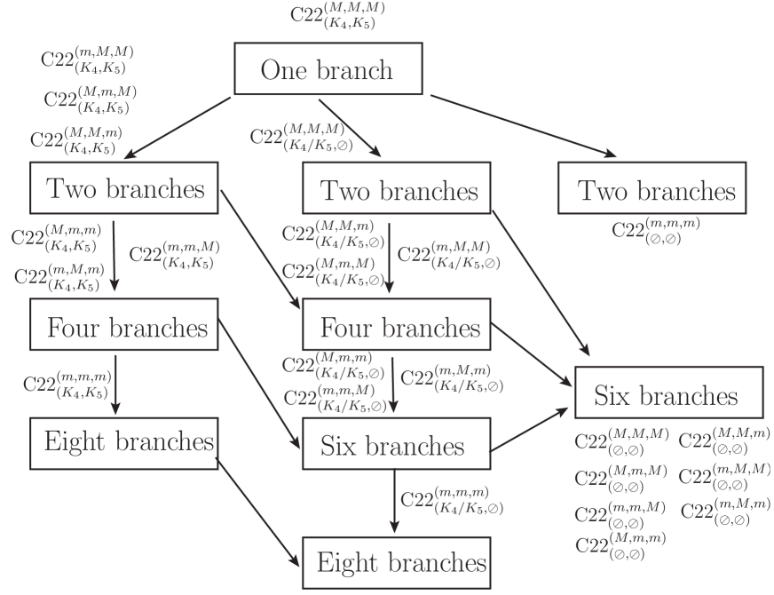
Figure 7: The splitting of variety into branches under different kinematic configurations. All branches are dimension two varieties, except the most degenerated case $\mbox{C22}^{(m,m,m)}_{(\oslash,\oslash)}$ where one branch is dimension four and the other, dimension three. The arrows indicate how branches split when one more specific kinematic condition is imposed.

7 Remaining two-loop topologies

After demonstrating methods and various properties with above planar penta-triangle and non-planar crossed double-triangle examples, we will present results for the remaining two-loop topologies in this section. We will omit many details but show only main results.

7.1 The topology (C32): non-planar crossed box-triangle

There is only one topology left for type (C), i.e., the crossed box-triangle topology (C32). We use $K_{1},K_{3}$ to construct momentum basis $e_{i}$. From seven on-shell equations, we can solve, for instance, $x_{1},x_{2},y_{1},y_{2}$ as linear functions of four ISPs $(x_{3},x_{4},y_{3},y_{4})$. The remaining three propagators are quadratic functions of ISPs. For general kinematic configuration, the expression and solution of cut equations are tedious, so we will not explicitly write them down here.

Integrand basis: In general, the variety defined by these three remaining quadratic cut equations is irreducible and dimension one. Using Gröbner basis method under ISPs ordering $(y_{4},y_{3},x_{4},x_{3})$ and the renormalization conditions

$$\sum_{\mbox{\tiny{all~{}ISPs~{}of~{}x}}}d(x_{i})\leq 5~{},~{}~{}~{}\sum_{\mbox{\tiny{all~{}ISPs~{}of~{}y}}}d(y_{i})\leq 4~{},~{}~{}~{}\sum_{\mbox{\tiny{all~{}ISPs~{}of~{}x}}}d(x_{i})+\sum_{\mbox{\tiny{all~{}ISPs~{}of~{}y}}}d(y_{i})\leq 6~{},~{}~{}~{}$$ (74)

we can get integrand basis for various kinematic configurations. There are all together four kinds of integrand basis depending on the massless limits of $K_{1},K_{3}$ since we have chosen $K_{1},K_{3}$ to generate momentum basis. For all kinematic configurations with $K_{1},K_{3}$ massive, the integrand basis contains 38 elements given by

$${\cal B}_{C32}^{I} = \{1,x_{3},x_{3}^{2},x_{3}^{3},x_{3}^{4},x_{3}^{5},x_{3}^{6},x_{4},x_{3}x_{4},x_{3}^{2}x_{4},x_{3}^{3}x_{4},x_{3}^{4}x_{4},x_{3}^{5}x_{4},y_{3},x_{3}y_{3},x_{3}^{2}y_{3},x_{3}^{3}y_{3},$$ (75)

$$x_{3}^{4}y_{3},x_{3}^{5}y_{3},x_{4}y_{3},x_{3}x_{4}y_{3},x_{3}^{2}x_{4}y_{3},x_{3}^{3}x_{4}y_{3},x_{3}^{4}x_{4}y_{3},y_{3}^{2},x_{3}y_{3}^{2},x_{4}y_{3}^{2},y_{3}^{3},x_{3}y_{3}^{3},x_{4}y_{3}^{3},$$

$$y_{3}^{4},x_{3}y_{3}^{4},x_{4}y_{3}^{4},y_{4},x_{3}y_{4},y_{3}y_{4},y_{3}^{2}y_{4},y_{3}^{3}y_{4}\}~{}.~{}~{}~{}$$

For all kinematic configurations with $K_{1}$ massless while $K_{3}$ massive, the integrand basis still contains 38 elements, and is given by replacing 9 elements in ${\cal B}_{C32}^{I}$

$${\cal B}_{C32}^{II} = {\cal B}_{C32}^{I}-\{x_{3}x_{4},x_{3}^{2}x_{4},x_{3}^{3}x_{4},x_{3}^{4}x_{4},x_{3}^{5}x_{4},x_{3}x_{4}y_{3},x_{3}^{2}x_{4}y_{3}x_{3}^{3}x_{4}y_{3},x_{3}^{4}x_{4}y_{3}\}$$ (76)

$$+\{x_{4}^{2},x_{4}^{3},x_{4}^{4},x_{4}^{5},x_{4}^{6},x_{4}^{2}y_{3},x_{4}^{3}y_{3},x_{4}^{4}y_{3},x_{4}^{5}y_{3}\}~{}.~{}~{}~{}$$

For all kinematic configurations with $K_{1}$ massive while $K_{3}$ massless, the integrand basis contains 38 elements, and is given by replacing 6 elements in ${\cal B}_{C32}^{I}$

$${\cal B}_{C32}^{III} = {\cal B}_{C32}^{I}-\{x_{4}y_{3}^{2},x_{4}y_{3}^{3},x_{4}y_{3}^{4},y_{3}y_{4},y_{3}^{2}y_{4},y_{3}^{3}y_{4}\}+\{y_{4}^{2},x_{3}y_{4}^{2},y_{4}^{3},x_{3}y_{4}^{3},y_{4}^{4},x_{3}y_{4}^{4}\}~{}.~{}~{}~{}$$ (77)

Finally for all kinematic configurations with both $K_{1},K_{3}$ massless, the 38 elements of integrand basis are given by replacing fifteen elements in ${\cal B}_{C32}^{I}$

$${\cal B}_{C32}^{IV} = {\cal B}_{C32}^{I}-\{x_{3}x_{4},x_{3}^{2}x_{4},x_{3}^{3}x_{4},x_{3}^{4}x_{4},x_{3}^{5}x_{4},x_{3}x_{4}y_{3},x_{3}^{2}x_{4}y_{3},x_{3}^{3}x_{4}y_{3},x_{3}^{4}x_{4}y_{3},$$ (78)

$$x_{4}y_{3}^{2},x_{4}y_{3}^{3},x_{4}y_{3}^{4},y_{3}y_{4},y_{3}^{2}y_{4},y_{3}^{3}y_{4}\}+\{x_{4}^{2},x_{4}^{3},x_{4}^{4},x_{4}^{5},x_{4}^{6},x_{4}^{2}y_{3},x_{4}^{3}y_{3},x_{4}^{4}y_{3},$$

$$x_{4}^{5}y_{3},y_{4}^{2},x_{3}y_{4}^{2},y_{4}^{3},x_{3}y_{4}^{3},y_{4}^{4},x_{3}y_{4}^{4}\}~{}.~{}~{}~{}$$

To discuss the structure of variety, we again use the notation $\mbox{C32}_{(U,P)}^{(L,N,R)}$ where now $U,P$ could either be $K_{5},K_{6}$ or $\oslash$ representing corresponding $K_{5},K_{6}$ absent. $L$ will be $m$ if at least one momentum of $K_{1},K_{2}$ is massless, and $R$ will be $m$ if $K_{3}$ is massless, while $N$ will be $m$ if $K_{4}$ is massless. Otherwise they will be $M$.

The number of branches under various kinematic configurations is summarized in table 1.

	$(K_{5},K_{6})$	$(K_{5}/K_{6},\oslash)$	$(\oslash,\oslash)$
$(M,M,M)$	1	2	4
$(m,M,M),(M,m,M),(M,M,m)$	2	4	6
$(m,m,M),(m,M,m),(M,m,m)$	4	6	6 for $(M,m,m)$/8
$(m,m,m)$	8	8	8

Table 1: Number of branches of various kinematic configurations for non-planar crossed box-triangle topology. The kinematic configurations are denoted by $\mbox{C32}_{(U,P)}^{(L,N,R)}$.

For each kinematic configuration, one should use all branches to find all 38 coefficients of integrand basis. We can also use branch-by-branch polynomial fitting method to simplify calculations.

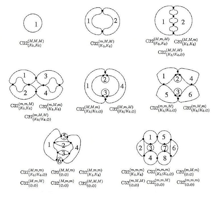
Figure 8: Intersections of branches for various kinematic configurations of non-planar crossed box-triangle topology (C32). Each branch $V_{i}$ is represented by a closed loop and denoted by $i$, while black dot is the intersecting point. Kinematic configurations for each pattern are listed below each diagram.

Variety with one branch: For the most general kinematics $\mbox{C32}_{(K_{5},K_{6})}^{(M,M,M)}$, the variety is irreducible with dimension one. All 38 coefficients should be found using this branch.

Variety with two branches: For kinematic configurations

$$\mbox{C32}_{(K_{5},K_{6})}^{(M,M,m)}~{},~{}\mbox{C32}_{(K_{5},K_{6})}^{(M,m,M)}~{},~{}\mbox{C32}_{(K_{5},K_{6})}^{(m,M,M)}~{},~{}\mbox{C32}_{(K_{5}/K_{6},\oslash)}^{(M,M,M)}~{},~{}~{}~{}$$ (79)

the variety is given by two branches with dimension one. These branches will intersect at points. More explicitly, for $\mbox{C32}_{(K_{5},K_{6})}^{(m,M,M)}$, two branches intersect at two isolated points, while for $\mbox{C32}_{(K_{5},K_{6})}^{(M,M,m)}$, $\mbox{C32}_{(K_{5},K_{6})}^{(M,m,M)}$ and $\mbox{C32}_{(K_{5}/K_{6},\oslash)}^{(M,M,M)}$, two branches intersect at four points.

Variety with four branches: For kinematic configurations

$$~{}\mbox{C32}_{(K_{5},K_{6})}^{(m,m,M)}~{},~{}\mbox{C32}_{(K_{5},K_{6})}^{(m,M,m)}~{},~{}\mbox{C32}_{(K_{5}/K_{6},\oslash)}^{(M,M,m)}~{},~{}\mbox{C32}_{(K_{5}/K_{6},\oslash)}^{(M,m,M)}~{},~{}\mbox{C32}_{(K_{5}/K_{6},\oslash)}^{(m,M,M)}~{},~{}~{}~{}~{}$$ (80)

the variety is given by four branches with dimension one. The intersection pattern among four branches $V_{1},V_{2},V_{3},V_{4}$ can be shown as follows. For $\mbox{C32}_{(K_{5},K_{6})}^{(m,m,M)}$, $\mbox{C32}_{(K_{5},K_{6})}^{(m,M,m)}$ and $\mbox{C32}_{(K_{5}/K_{6},\oslash)}^{(m,M,M)}$, the only non-zero intersections are given by $V_{1}\cap V_{2}=V_{3}\cap V_{4}=(0|2)$, $V_{1}\cap V_{3}=V_{2}\cap V_{4}=(0|1)$. For $\mbox{C32}_{(K_{5}/K_{6},\oslash)}^{(M,M,m)}$ and $\mbox{C32}_{(K_{5}/K_{6},\oslash)}^{(M,m,M)}$, non-zero intersections are given by $V_{1}\cap V_{4}=(0|2)$, $V_{1}\cap V_{2}=V_{2}\cap V_{4}=(0|1)$, $V_{1}\cap V_{3}=V_{3}\cap V_{4}=(0|1)$.

Variety with six branches: For kinematic configurations

$$\mbox{C32}_{(K_{5},K_{6})}^{(M,m,m)}~{},~{}\mbox{C32}_{(\oslash,\oslash)}^{(M,M,M)}~{},~{}\mbox{C32}_{(K_{5}/K_{6},\oslash)}^{(m,M,m)}~{},~{}\mbox{C32}_{(K_{5}/K_{6},\oslash)}^{(m,m,M)}~{},~{}$$

$$\mbox{C32}_{(K_{5}/K_{6},\oslash)}^{(M,m,m)}~{},~{}\mbox{C32}_{(\oslash,\oslash)}^{(M,M,m)}~{},~{}\mbox{C32}_{(\oslash,\oslash)}^{(M,m,M)}~{},~{}\mbox{C32}_{(\oslash,\oslash)}^{(M,m,m)}~{},~{}~{}~{}$$ (81)

the variety is given by six branches with dimension one. These branches again intersect at points. For $\mbox{C32}_{(K_{5}/K_{6},\oslash)}^{(m,M,m)}$ and $\mbox{C32}_{(K_{5}/K_{6},\oslash)}^{(m,m,M)}$, each pair of $(V_{1},V_{2})$, $(V_{2},V_{4})$, $(V_{4},V_{1})$, $(V_{5},V_{6})$, $(V_{6},V_{3})$, $(V_{3},V_{5})$, $(V_{1},V_{5})$, $(V_{4},V_{6})$ intersects at one single point. For $\mbox{C32}_{(K_{5},K_{6})}^{(M,m,m)}$, $\mbox{C32}_{(\oslash,\oslash)}^{(M,M,M)}$, $\mbox{C32}_{(K_{5}/K_{6},\oslash)}^{(M,m,m)}$, $\mbox{C32}_{(\oslash,\oslash)}^{(M,M,m)}$, $\mbox{C32}_{(\oslash,\oslash)}^{(M,m,M)}$ and $\mbox{C32}_{(\oslash,\oslash)}^{(M,m,m)}$, each pair of $(V_{1},V_{i})$ and $(V_{4},V_{i})$ for $i=2,3,5,6$ intersects at one single point.

Variety with eight branches: For kinematic configurations

$$\mbox{C32}_{(K_{5},K_{6})}^{(m,m,m)}~{},~{}\mbox{C32}_{(K_{5}/K_{6},\oslash)}^{(m,m,m)}~{},~{}\mbox{C32}_{(\oslash,\oslash)}^{(m,M,m)}~{},~{}\mbox{C32}_{(\oslash,\oslash)}^{(m,m,M)}~{},~{}\mbox{C32}_{(\oslash,\oslash)}^{(m,m,m)}~{},~{}\mbox{C32}_{(\oslash,\oslash)}^{(m,M,M)}~{},~{}~{}~{}~{}$$ (82)

the variety is given by eight branches with dimension one. There will be single intersecting point for each pair of following ten combinations: $(V_{1},V_{2})$, $(V_{1},V_{3})$, $(V_{1},V_{5})$, $(V_{2},V_{4})$, $(V_{3},V_{4})$, $(V_{4},V_{8})$, $(V_{5},V_{6})$, $(V_{5},V_{7})$, $(V_{6},V_{8})$ and $(V_{7},V_{8})$.

The intersection pattern of branches for each kinematic configurations is shown in Figure (8).

7.2 The topology (B41): planar penta-bubble

From on-shell equations of six propagators we can get three linear equations for pure $\ell_{1}$, and reduce four RSPs $(x_{1},x_{2},x_{3},x_{4})$ to one. Exception happens when $K_{4}=K_{5}=0$, $D_{4}=(\ell_{1}-K_{1}-K_{2}-K_{3})^{2}=\ell_{1}^{2}$ from momentum conservation, and the independent linear equations containing pure $\ell_{1}$ reduce to two. In this case we get two ISPs from $x_{i}$. There is no linear equation for pure $\ell_{2}$, so all four $y_{i}$ are ISPs. Adding them together there will be 5 ISPs (or 6 ISPs for the case $K_{4}=K_{5}=0$).

We use $K_{1},K_{3}$ to construct momentum basis $e_{i}$. After solving linear equations we can express remaining three quadratic equations with ISPs. Using Gröbner basis method with ISPs’ ordering $(x_{4},y_{1},y_{2},y_{3},y_{4})$ for kinematic configurations $\mbox{B41}_{(K_{4},K_{5})}$, $\mbox{B41}_{(K_{4}/K_{5},\oslash)}$ under renormalization conditions

$$\sum_{\mbox{\tiny{all~{}ISPs~{}of~{}x}}}d(x_{i})\leq 5~{},~{}~{}~{}\sum_{\mbox{\tiny{all~{}ISPs~{}of~{}y}}}d(y_{i})\leq 2~{},~{}~{}~{}\sum_{\mbox{\tiny{all~{}ISPs~{}of~{}x}}}d(x_{i})+\sum_{\mbox{\tiny{all~{}ISPs~{}of~{}y}}}d(y_{i})\leq 5~{}.~{}~{}$$ (83)

we can get integrand basis with $18$ elements. We have three kinds of integrand basis for kinematic configurations $\mbox{B41}_{(K_{4},K_{5})}$, $\mbox{B41}_{(K_{4}/K_{5},\oslash)}$ according to kinematics of $K_{1},K_{3}$ since we have chose $K_{1},K_{3}$ to generate momentum basis. The first kind is suitable for all kinematic configurations of $\mbox{B41}_{(K_{4},K_{5})}$, or $K_{3}$ massive while others arbitrary for $\mbox{B41}_{(K_{4},\oslash)}$, or $K_{1}$ massive while others arbitrary for $\mbox{B41}_{(K_{5},\oslash)}$. It is given by 18 elements

$$\mathcal{B}_{B41}^{I}=\{1,x_{4},y_{1},y_{2},x_{4}y_{2},y_{2}^{2},y_{3},y_{1}y_{3},y_{2}y_{3},y_{3}^{2},y_{4},x_{4}y_{4},y_{1}y_{4},y_{2}y_{4},x_{4}y_{2}y_{4},y_{3}y_{4},y_{4}^{2},x_{4}y_{4}^{2}\}~{}.~{}~{}~{}$$ (84)

The second kind is suitable for kinematic configurations with $K_{1}$ massless while others arbitrary for $\mbox{B41}_{(K_{5},\oslash)}$. The 18 elements of integrand basis are given by replacing one element in $\mathcal{B}_{B41}^{I}$

$$\mathcal{B}_{B41}^{II}=\mathcal{B}_{B4}^{I}-\{x_{4}y_{2}y_{4}\}+\{x_{4}y_{2}^{2}\}~{}.~{}~{}~{}$$ (85)

The third kind is suitable for kinematic configurations with $K_{3}$ massless while others arbitrary for $\mbox{B41}_{(K_{4},\oslash)}$. The 18 elements of integrand basis are given by replacing three elements in $\mathcal{B}_{B41}^{I}$

$$\mathcal{B}_{B41}^{III}=\mathcal{B}_{B41}^{I}-\{x_{4}y_{2},y_{2}^{2},x_{4}y_{2}y_{4}\}+\{x_{4}y_{1},y_{1}^{2},x_{4}y_{1}^{2}\}~{}.~{}~{}~{}$$ (86)

For all kinematic configurations of $\mbox{B41}_{(\oslash,\oslash)}$ where ISPs are given by six variables with ordering $(x_{3},x_{4},y_{1},y_{2},y_{3},y_{4})$, we get 83 elements for integrand basis

$$\mathcal{B}_{B41}^{IV} = \{1,x_{3},x_{3}^{2},x_{3}^{3},x_{3}^{4},x_{3}^{5},x_{4},x_{4}^{2},x_{4}^{3},x_{4}^{4},x_{4}^{5},y_{1},x_{3}y_{1},x_{3}^{2}y_{1},x_{3}^{3}y_{1},x_{3}^{4}y_{1},x_{4}y_{1},x_{4}^{2}y_{1},x_{4}^{3}y_{1},x_{4}^{4}y_{1},$$ (87)

$$y_{1}^{2},x_{3}y_{1}^{2},x_{3}^{2}y_{1}^{2},x_{3}^{3}y_{1}^{2},x_{4}y_{1}^{2},x_{4}^{2}y_{1}^{2},x_{4}^{3}y_{1}^{2},y_{2},x_{3}y_{2},x_{3}^{2}y_{2},x_{3}^{3}y_{2},x_{3}^{4}y_{2},x_{4}y_{2},x_{4}^{2}y_{2},x_{4}^{3}y_{2},x_{4}^{4}y_{2},$$

$$y_{2}^{2},x_{3}y_{2}^{2},x_{3}^{2}y_{2}^{2},x_{3}^{3}y_{2}^{2},x_{4}y_{2}^{2},x_{4}^{2}y_{2}^{2},x_{4}^{3}y_{2}^{2},y_{3},x_{3}y_{3},x_{3}^{2}y_{3},x_{3}^{3}y_{3},x_{3}^{4}y_{3},x_{4}y_{3},y_{1}y_{3},x_{3}y_{1}y_{3},$$

$$x_{3}^{2}y_{1}y_{3},x_{3}^{3}y_{1}y_{3},x_{4}y_{1}y_{3},y_{2}y_{3},x_{3}y_{2}y_{3},x_{3}^{2}y_{2}y_{3},x_{3}^{3}y_{2}y_{3},x_{4}y_{2}y_{3},y_{3}^{2},x_{3}y_{3}^{2},x_{3}^{2}y_{3}^{2},x_{3}^{3}y_{3}^{2},x_{4}y_{3}^{2},$$

$$y_{4},x_{4}y_{4},x_{4}^{2}y_{4},x_{4}^{3}y_{4},x_{4}^{4}y_{4},y_{1}y_{4},x_{4}y_{1}y_{4},x_{4}^{2}y_{1}y_{4},x_{4}^{3}y_{1}y_{4},y_{2}y_{4},x_{4}y_{2}y_{4},x_{4}^{2}y_{2}y_{4},x_{4}^{3}y_{2}y_{4},$$

$$y_{3}y_{4},x_{4}y_{3}y_{4},y_{4}^{2},x_{4}y_{4}^{2},x_{4}^{2}y_{4}^{2},x_{4}^{3}y_{4}^{2}\}~{}.~{}~{}~{}$$

The reason we have 83 elements instead of 18 is that, for $\mbox{B41}_{(K_{4},K_{5})}$ and $\mbox{B41}_{(K_{4}/K_{5},\oslash)}$, $x_{4}$ is determined by quadratic equation, i.e., the maximal power of $x_{4}$ is two, while for $\mbox{B41}_{(\oslash,\oslash)}$ we can have $d(x_{3})+d(x_{4})\leq 5$.

In order to simplify the calculations of coefficients, we need to discuss the branch structure of variety. For $\mbox{B41}_{(K_{4},K_{5})}$ and $\mbox{B41}_{(K_{4}/K_{5},\oslash)}$, there is a quadratic equation of single variable $x_{4}$, and we can always get two solutions of $x_{4}$ in $\mathbb{C}$-plane no matter what the momentum configuration of $K_{1},K_{2},K_{3}$ is. Thus there will always be two separate branches characterized by two solutions $x_{4}^{\Gamma_{1}},x_{4}^{\Gamma_{2}}$. For $\mbox{B41}_{(K_{4},K_{5})}$, these two branches with dimension two will not split further. Using each branch we can detect 9 coefficients of integrand basis, and since there is no intersection between two branches, we can detect all $9+9=18$ coefficients using both branches. For $\mbox{B41}_{(K_{4}/K_{5},\oslash)}$, each branch will split further into two branches, so there will be in total four branches: $V_{1},V_{2}$ characterized by $x_{4}^{\Gamma_{1}}$ and $V_{3},V_{4}$ characterized by $x_{4}^{\Gamma_{2}}$. Each branch can detect 6 coefficients. The two branches characterized by $x_{4}^{\Gamma_{i}}$ will intersect at one-dimensional variety with intersection pattern $(1|3)=V_{1}\cap V_{2}$ and $(1|3)=V_{3}\cap V_{4}$. So using two branches of each $x_{4}^{\Gamma_{i}}$ we can detect $6+6-3=9$ coefficients, and in total $9+9=18$ coefficients using all 4 branches.

For kinematic configurations $\mbox{B41}_{(\oslash,\oslash)}$, $x_{3},x_{4}$ are both ISPs, so the quadratic equation of $(x_{3},x_{4})$ could not be factorized into two separate pieces in general. If all $K_{1},K_{2},K_{3}$ are massive, the variety is given by two branches. Each branch is 3-dimensional, and the intersection of these two branches is 2-dimensional. Each branch can detect 58 coefficients, while the intersection of them is $(2|33)=V_{1}\cap V_{2}$. If at least one momentum of $K_{1},K_{3}$ is massive, the variety will split into four 3-dimensional branches $V_{1},V_{2}$ and $V_{3},V_{4}$. Using $V_{1}$ or $V_{3}$ we can detect 28 coefficients of integrand basis, while using $V_{2}$ or $V_{4}$ we can detect 36 coefficients. The intersection of these four branches is 1-dimensional, and it can detect 3 coefficients. Intersections of every three branches are also the same 1-dimensional variety as the one given by intersection of four branches. For intersections of every two branches, $(V_{1},V_{3})$ and $(V_{2},V_{4})$ are inherited from the intersection of four branches, which is 1-dimensional variety. The intersections of $(V_{1},V_{4})$ and $(V_{2},V_{3})$ are 2-dimensional. Their intersection pattern is $(2|6)=V_{1}\cap V_{4}$, $(2|6)=V_{2}\cap V_{3}$. The intersections of $(V_{1},V_{2})$ and $(V_{3},V_{4})$ are also 2-dimensional, from which 18 coefficients can be detected using each intersection.

For the special kinematic configuration of $\mbox{B41}_{(\oslash,\oslash)}$ with both $K_{1},K_{3}$ massless, the three quadratic on-shell equations reduce to

$$x_{3}x_{4}=0~{},~{}~{}~{}y_{1}y_{2}+y_{3}y_{4}=0~{},~{}~{}~{}x_{3}y_{4}+x_{4}y_{3}=0~{}.~{}~{}~{}$$ (88)

Besides the ordinary four branches

$$V_{1}:~{}~{}~{}x_{3}=0~{},~{}y_{2}=0~{},~{}y_{3}=0~{},~{}x_{4}~{},~{}y_{1}~{},~{}y_{4}~{},~{}\mbox{free parameters}~{},~{}~{}~{}$$

$$V_{2}:~{}~{}~{}x_{3}=0~{},~{}y_{1}=0~{},~{}y_{3}=0~{},~{}x_{4}~{},~{}y_{2}~{},~{}y_{4}~{},~{}\mbox{free parameters}~{},~{}~{}~{}$$

$$V_{3}:~{}~{}~{}x_{4}=0~{},~{}y_{2}=0~{},~{}y_{4}=0~{},~{}x_{3}~{},~{}y_{1}~{},~{}y_{3}~{},~{}\mbox{free parameters}~{},~{}~{}~{}$$

$$V_{4}:~{}~{}~{}x_{4}=0~{},~{}y_{1}=0~{},~{}y_{4}=0~{},~{}x_{3}~{},~{}y_{2}~{},~{}y_{3}~{},~{}\mbox{free parameters}~{},~{}~{}~{}$$ (89)

there is also another embedded branch given by the ideal

$$V_{5}:~{}~{}~{}\{x_{4}y_{3}+x_{3}y_{4},y_{1}y_{2}+y_{3}y_{4},x_{4}^{2},x_{3}x_{4},x_{3}^{2}\}~{}.~{}~{}~{}$$ (90)

Each of the ordinary branches can detect 28 coefficients, while $V_{5}$ can detect 37 coefficients. These five branches intersect at one single point, and intersections of every four branches are also the same point. For intersections of every three branches, we have $(1|6)=(V_{1},V_{2},V_{5})$, $(1|6)=(V_{3},V_{4},V_{5})$, $(1|3)=(V_{1},V_{3},V_{5})$, $(1|3)=(V_{2},V_{4},V_{5})$, and they are all different 1-dimensional varieties. The other intersections of every three branches are inherited from the same point of intersection of five branches. For intersections of every two branches, $(V_{1},V_{4})$, $(V_{2},V_{3})$ are at the same point of intersection of five branches, while $(V_{1},V_{3})$, $(V_{2},V_{4})$ are the same 1-dimensional varieties of intersections of $(V_{1},V_{3},V_{5})$ and $(V_{2},V_{4},V_{5})$ respectively. Intersections of other combinations of pairs are 2-dimensional and we have $(2|12)=V_{1}\cap V_{5}$, $(2|12)=V_{2}\cap V_{5}$, $(2|12)=V_{3}\cap V_{5}$, $(2|12)=V_{4}\cap V_{5}$, $(2|15)=V_{1}\cap V_{2}$, $(2|15)=V_{3}\cap V_{4}$. They are all different 2-dimensional varieties.

7.3 The topology (B33): planar double-box

This topology has been discussed in details in many other papers[21, 22, 23, 24], here we will briefly summarize some results. We use $K_{1},K_{4}$ to construct momentum basis $e_{i},i=1,2,3,4$ and all kinematics can be expanded by this basis. The seven on-shell equations can be reduced to three quadratic equations with four variables after solving four linear equations. Since there are two linear equations for $x_{i}$ variables and two for $y_{i}$, by solving them we can get 4 ISPs $(x_{2},x_{4},y_{1},y_{4})$ for instance. Then $D_{0}=0$ becomes a conic section of $(x_{2},x_{4})$, $\widetilde{D}_{0}=0$ becomes a conic section of $(y_{1},y_{4})$ and $\widehat{D}_{0}=0$ is a quadratic equation of $(x_{2},x_{4},y_{1},y_{4})$. Variety defined by these three quadratic equations will be reducible if any of $K_{1},K_{2},K_{3},K_{4}$ is massless, or any of $K_{5},K_{6}$ is zero.

The renormalization conditions

$$\sum_{\mbox{\tiny{all~{}ISPs~{}of~{}x}}}d(x_{i})\leq 4~{},~{}\sum_{\mbox{\tiny{all~{}ISPs~{}of~{}y}}}d(y_{i})\leq 4~{},~{}\sum_{\mbox{\tiny{all~{}ISPs~{}of~{}x}}}d(x_{i})+\sum_{\mbox{\tiny{all~{}ISPs~{}of~{}y}}}d(y_{i})\leq 6~{}~{}~{}~{}$$ (91)

constrain all possible monomials $x_{2}^{d(x_{2})}x_{4}^{d(x_{4})}y_{1}^{d(y_{1})}y_{4}^{d(y_{4})}$. We can get 32 elements for integrand basis after dividing them by Gröbner basis generated from three quadratic equations with ISPs’ ordering $(x_{2},x_{4},y_{1},y_{4})$. Integrand basis for different kinematic configurations can be arranged to four kinds according to the kinematics of $K_{1},K_{4}$, which we have chosen to generate momentum basis $e_{i}$. If $K_{1},K_{4}$ are massive, integrand basis is given by following $32$ elements

$$\mathcal{B}_{B33}^{I} = \{1,x_{2},x_{4},x_{2}x_{4},x_{4}^{2},x_{2}x_{4}^{2},x_{4}^{3},x_{2}x_{4}^{3},x_{4}^{4},y_{1},x_{4}y_{1},x_{4}^{2}y_{1},x_{4}^{3}y_{1},x_{4}^{4}y_{1},y_{4},x_{2}y_{4},x_{4}y_{4},x_{4}^{2}y_{4},$$ (92)

$$x_{4}^{3}y_{4},x_{4}^{4}y_{4},y_{1}y_{4},x_{4}y_{1}y_{4},y_{4}^{2},x_{4}y_{4}^{2},y_{1}y_{4}^{2},x_{4}y_{1}y_{4}^{2},y_{4}^{3},x_{4}y_{4}^{3},y_{1}y_{4}^{3},x_{4}y_{1}y_{4}^{3},y_{4}^{4},x_{4}y_{4}^{4}\}~{}.~{}~{}~{}$$

If $K_{1}$ is massless while $K_{4}$ is massive, integrand basis is given by replacing 6 elements in $\mathcal{B}_{B33}^{I}$ as follows

$$\mathcal{B}_{B33}^{II}=\mathcal{B}_{B33}^{I}-\{x_{2}x_{4},x_{2}x_{4}^{2},x_{2}x_{4}^{3},x_{4}^{2}y_{1},x_{4}^{3}y_{1},x_{4}^{4}y_{1}\}+\{x_{2}^{2},x_{2}^{3},x_{2}^{4},x_{2}^{2}y_{4},x_{2}^{3}y_{4},x_{2}^{4}y_{4}\}~{}.~{}~{}~{}$$ (93)

If $K_{4}$ is massless while $K_{1}$ is massive, integrand basis is given by replacing 6 elements in $\mathcal{B}_{B33}^{I}$ as follows

$$\mathcal{B}_{B33}^{III}=\mathcal{B}_{B33}^{I}-\{y_{1}y_{4},x_{4}y_{1}y_{4},y_{1}y_{4}^{2},x_{4}y_{1}y_{4}^{2},y_{1}y_{4}^{3},x_{4}y_{1}y_{4}^{3}\}+\{y_{1}^{2},x_{4}y_{1}^{2},y_{1}^{3},x_{4}y_{1}^{3},y_{1}^{4},x_{4}y_{1}^{4}\}~{}.~{}~{}~{}$$ (94)

Finally if both $K_{1},K_{4}$ are massless, integrand basis is given by replacing 12 elements in $\mathcal{B}_{B33}^{I}$, which are exactly 6 elements from the second kind of integrand basis plus the other 6 elements from the third kind of integrand basis

$$\mathcal{B}_{B33}^{IV} = \{1,x_{2},x_{2}^{2},x_{2}^{3},x_{2}^{4},x_{4},x_{4}^{2},x_{4}^{3},x_{4}^{4},y_{1},x_{4}y_{1},y_{1}^{2},x_{4}y_{1}^{2},y_{1}^{3},x_{4}y_{1}^{3},y_{1}^{4},x_{4}y_{1}^{4},y_{4},$$ (95)

$$x_{2}y_{4},x_{2}^{2}y_{4},x_{2}^{3}y_{4},x_{2}^{4}y_{4},x_{4}y_{4},x_{4}^{2}y_{4},x_{4}^{3}y_{4},x_{4}^{4}y_{4},y_{4}^{2},x_{4}y_{4}^{2},y_{4}^{3},x_{4}y_{4}^{3},y_{4}^{4},x_{4}y_{4}^{4}\}~{}.~{}~{}~{}$$

We use notation $\mbox{B33}_{(U,P)}^{(L,R)}$ to denote different kinematic configurations, where again $U,P$ could be either $K_{5},K_{6}$ or $\oslash$, and $L$ is denoted by $m$ if at least one momentum of $K_{1},K_{2}$ (or $K_{3},K_{4}$ for $R$) is massless, otherwise it will be denoted by $M$.

For general kinematic configuration $\mbox{B33}_{(K_{5},K_{6})}^{(M,M)}$, the variety is irreducible with dimension one. For kinematic configurations $\mbox{B33}_{(K_{5},K_{6})}^{(m,M)}$, $\mbox{B33}_{(K_{5},K_{6})}^{(M,m)}$, $\mbox{B33}_{(K_{5}/K_{6},\oslash)}^{(M,M)}$ and $\mbox{B33}_{(\oslash,\oslash)}^{(M,M)}$, the variety splits into two branches. Each branch can detect 17 coefficients of integrand basis, and two branches intersect at two points, which exactly gives $17+17-2=32$ coefficients when using both two branches.

For $\mbox{B33}_{(K_{5},K_{6})}^{(m,m)}$, the variety is given by four branches. Each branch can detect 9 coefficients. There is no intersection for four branches or every three branches, while each of following pairs $(V_{1},V_{2})$, $(V_{2},V_{3})$, $(V_{3},V_{4})$ and $(V_{4},V_{1})$ intersects at a single point. Thus when combining them together we can find $9\times 4-4=32$ coefficients. For kinematic configurations $\mbox{B33}_{(K_{5}/K_{6},\oslash)}^{(m,M)}$ , $\mbox{B33}_{(K_{5}/K_{6},\oslash)}^{(M,m)}$, $\mbox{B33}_{(\oslash,\oslash)}^{(m,M)}$ and $\mbox{B33}_{(\oslash,\oslash)}^{(M,m)}$, the variety is also given by four branches. Branches $V_{1},V_{3}$ can detect 5 coefficients individually while branches $V_{2},V_{4}$ can detect 13 coefficients individually. The non-zero intersections among branches are still single points between following pairs $(V_{1},V_{2})$, $(V_{2},V_{3})$, $(V_{3},V_{4})$, $(V_{4},V_{1})$.

For kinematic configurations $\mbox{B33}_{(K_{5}/K_{6},\oslash)}^{(m,m)}$ and $\mbox{B33}_{(\oslash,\oslash)}^{(m,m)}$, the variety is given by six branches. Among these six branches, $V_{1},V_{4}$ can detect $9$ coefficients while $V_{2},V_{3},V_{5},V_{6}$ can detect 5 coefficients. Non-zero intersections exist only for following pairs $(V_{1},V_{2})$, $(V_{2},V_{3})$, $(V_{3},V_{4})$, $(V_{4},V_{5})$, $(V_{5},V_{6})$ and $(V_{6},V_{1})$, and each intersection is a single point. So using all six branches we can detect $2\times 9+4\times 5-6=32$ coefficients.

Results presented here are consistent with those found in [21, 22, 23, 24]. In our discussion, the variety will be reducible for kinematic configurations that any of $K_{1},K_{2},K_{3}$ $K_{4}$ is massless, or any of $K_{5},K_{6}$ is zero. These configurations correspond to the existence of three-vertex $\oplus$ or $\ominus$. The distribution of $\oplus$ and $\ominus$ will generate different kinematical solutions to the heptacut constraints, which, in our language, are irreducible branches of the variety after primary decomposition. Each irreducible branch can be seen as a Riemann sphere, and the intersecting points between two branches is precisely the poles of heptacut Jacobian. According to these mapping, we can reconstruct the global structures of double-box topology shown in the references from irreducible branches and their intersections. The 32 elements of integrand basis are sufficient to expand double-box amplitude at the integrand-level, yet they are still redundant after loop integration. Only after eliminating the redundancy using IBP method for instance can we get integral basis shown in [21].

7.4 The topology (B32): planar box-triangle

For this topology, we can get two linear equations for $(x_{1},x_{2},x_{3},x_{4})$ and one linear equation for $(y_{1},y_{2},y_{3},y_{4})$, and reduce 8 RSPs to 5 ISPs $(x_{3},x_{4},y_{1},y_{3},y_{4})$. We use $K_{1},K_{3}$ to construct momentum basis $e_{i}$. Under the renormalization conditions

$$\sum_{\mbox{\tiny{all~{}ISPs~{}of~{}x}}}d(x_{i})\leq 4~{},~{}~{}~{}\sum_{\mbox{\tiny{all~{}ISPs~{}of~{}y}}}d(y_{i})\leq 3~{},~{}~{}~{}\sum_{\mbox{\tiny{all~{}ISPs~{}of~{}x}}}d(x_{i})+\sum_{\mbox{\tiny{all~{}ISPs~{}of~{}y}}}d(y_{i})\leq 5~{}~{}~{}$$ (96)

we can get integrand basis using the Gröbner basis with ordering $(x_{3},x_{4},y_{1},y_{3},y_{4})$. For $\mbox{B32}_{(K_{4},K_{5})}$ and $\mbox{B32}_{(K_{4}/K_{5},\oslash)}$, we get 69 elements for integrand basis, but these elements may be different. The difference can be classified by the kinematics of $K_{1},K_{3}$, and there are in total 4 kinds of integrand basis. The first kind is for all configurations with $K_{1},K_{3}$ massive, and the 69 elements are given by

$$\mathcal{B}_{B32}^{I} = \{1,x_{3},x_{4},x_{3}x_{4},x_{4}^{2},x_{3}x_{4}^{2},x_{4}^{3},x_{3}x_{4}^{3},x_{4}^{4},y_{1},x_{4}y_{1},x_{4}^{2}y_{1},x_{4}^{3}y_{1},x_{4}^{4}y_{1},y_{3},x_{3}y_{3},x_{4}y_{3},x_{4}^{2}y_{3},$$

$$x_{4}^{3}y_{3},x_{4}^{4}y_{3},y_{1}y_{3},x_{4}y_{1}y_{3},y_{3}^{2},x_{3}y_{3}^{2},x_{4}y_{3}^{2},x_{4}^{2}y_{3}^{2},x_{4}^{3}y_{3}^{2},y_{1}y_{3}^{2},x_{4}y_{1}y_{3}^{2},y_{3}^{3},x_{3}y_{3}^{3},x_{4}y_{3}^{3},x_{4}^{2}y_{3}^{3},$$ (97)

$$y_{4},x_{3}y_{4},x_{4}y_{4},x_{3}x_{4}y_{4},x_{4}^{2}y_{4},x_{3}x_{4}^{2}y_{4},x_{4}^{3}y_{4},x_{3}x_{4}^{3}y_{4},x_{4}^{4}y_{4},y_{1}y_{4},x_{4}y_{1}y_{4},x_{4}^{2}y_{1}y_{4},x_{4}^{3}y_{1}y_{4},$$

$$y_{3}y_{4},x_{4}y_{3}y_{4},x_{4}^{2}y_{3}y_{4},x_{4}^{3}y_{3}y_{4},y_{1}y_{3}y_{4},x_{4}y_{1}y_{3}y_{4},y_{3}^{2}y_{4},x_{4}y_{3}^{2}y_{4},x_{4}^{2}y_{3}^{2}y_{4},y_{4}^{2},x_{3}y_{4}^{2},x_{4}y_{4}^{2},$$

$$x_{4}^{2}y_{4}^{2},x_{4}^{3}y_{4}^{2},y_{1}y_{4}^{2},x_{4}y_{1}y_{4}^{2},y_{3}y_{4}^{2},x_{4}y_{3}y_{4}^{2},x_{4}^{2}y_{3}y_{4}^{2},y_{4}^{3},x_{3}y_{4}^{3},x_{4}y_{4}^{3},x_{4}^{2}y_{4}^{3}\}~{}.~{}~{}~{}$$

The second kind is for configurations with $K_{1}$ massless while $K_{3}$ massive, and the 69 elements are given by replacing 15 elements in $\mathcal{B}_{B32}^{I}$

$$\mathcal{B}_{B32}^{II} = \mathcal{B}_{B32}^{I}-\{x_{3}x_{4},x_{3}x_{4}^{2},x_{3}x_{4}^{3},x_{4}^{2}y_{1},x_{4}^{3}y_{1},x_{4}^{4}y_{1},x_{4}^{2}y_{3}^{2},x_{4}^{3}y_{3}^{2},x_{4}^{2}y_{3}^{3},x_{3}x_{4}y_{4},x_{3}x_{4}^{2}y_{4},$$ (98)

$$x_{3}x_{4}^{3}y_{4},x_{4}^{2}y_{1}y_{4},x_{4}^{3}y_{1}y_{4},x_{4}^{2}y_{3}^{2}y_{4}\}+\{x_{3}^{2},x_{3}^{3},x_{3}^{4},x_{3}^{2}y_{3},x_{3}^{3}y_{3},x_{3}^{4}y_{3},x_{3}^{2}y_{3}^{2},x_{3}^{3}y_{3}^{2},$$

$$x_{3}^{2}y_{3}^{3},x_{3}^{2}y_{4},x_{3}^{3}y_{4},x_{3}^{4}y_{4},x_{3}^{2}y_{4}^{2},x_{3}^{3}y_{4}^{2},x_{3}^{2}y_{4}^{3}\}~{}.~{}~{}~{}$$

The third kind is for configurations with $K_{3}$ massless while $K_{1}$ massive, and the 69 elements are given by replacing 12 elements in $\mathcal{B}_{B32}^{I}$

$$\mathcal{B}_{B32}^{III} = \mathcal{B}_{B32}^{I}-\{y_{3}y_{4},x_{4}y_{3}y_{4},x_{4}^{2}y_{3}y_{4},x_{4}^{3}y_{3}y_{4},y_{1}y_{3}y_{4},x_{4}y_{1}y_{3}y_{4},y_{3}^{2}y_{4},x_{4}y_{3}^{2}y_{4},x_{4}^{2}y_{3}^{2}y_{4},$$ (99)

$$y_{3}y_{4}^{2},x_{4}y_{3}y_{4}^{2},x_{4}^{2}y_{3}y_{4}^{2}\}+\{y_{1}^{2},x_{4}y_{1}^{2},y_{1}^{3},x_{4}y_{1}^{3},x_{4}^{2}y_{1}y_{3},x_{4}^{3}y_{1}y_{3},y_{1}^{2}y_{3},x_{4}y_{1}^{2}y_{3},$$

$$x_{4}^{2}y_{1}y_{3}^{2},y_{1}^{2}y_{4},x_{4}y_{1}^{2}y_{4},x_{4}^{2}y_{1}y_{4}^{2}\}~{}.~{}~{}~{}$$

The last kind of integrand basis is for configurations with $K_{1},K_{3}$ massless, and the 69 elements are given by replacing 23 elements in $\mathcal{B}_{B32}^{I}$

$$\mathcal{B}_{B32}^{IV} = \mathcal{B}_{B32}^{I}-\{x_{3}x_{4},x_{3}x_{4}^{2},x_{3}x_{4}^{3},x_{4}^{2}y_{1},x_{4}^{3}y_{1},x_{4}^{4}y_{1},x_{3}x_{4}y_{4},x_{3}x_{4}^{2}y_{4},x_{3}x_{4}^{3}y_{4},x_{4}^{2}y_{1}y_{4},x_{4}^{3}y_{1}y_{4},$$ (100)

$$y_{3}y_{4},x_{4}y_{3}y_{4},x_{4}^{2}y_{3}y_{4},x_{4}^{3}y_{3}y_{4},y_{1}y_{3}y_{4},x_{4}y_{1}y_{3}y_{4},y_{3}^{2}y_{4},x_{4}y_{3}^{2}y_{4},x_{4}^{2}y_{3}^{2}y_{4},y_{3}y_{4}^{2},x_{4}y_{3}y_{4}^{2},$$

$$x_{4}^{2}y_{3}y_{4}^{2}\}+\{x_{3}^{2},x_{3}^{3},x_{3}^{4},y_{1}^{2},x_{4}y_{1}^{2},y_{1}^{3},x_{4}y_{1}^{3},x_{3}^{2}y_{3},x_{3}^{3}y_{3},x_{3}^{4}y_{3},y_{1}^{2}y_{3},x_{4}y_{1}^{2}y_{3},x_{3}^{2}y_{3}^{2},x_{3}^{3}y_{3}^{2},$$

$$x_{3}^{2}y_{3}^{3},x_{3}^{2}y_{4},x_{3}^{3}y_{4},x_{3}^{4}y_{4},y_{1}^{2}y_{4},x_{4}y_{1}^{2}y_{4},x_{3}^{2}y_{4}^{2},x_{3}^{3}y_{4}^{2},x_{3}^{2}y_{4}^{3}\}~{}.~{}~{}~{}$$

The integrand basis for $\mbox{B32}_{(\oslash,\oslash)}$ can be distinguished by kinematics of $K_{3}$. If $K_{3}$ is massive, we still get 69 elements, while if $K_{3}$ is massless, we can get 77 elements instead of 69. The number of elements changes because in the specific momentum configuration, the sub-triangle-loop is 0m-triangle, so variety is 3-dimensional, while in other momentum configurations the variety is 2-dimensional. The 69 elements for $K_{3}$ massive case are given by

$$\mathcal{B}_{B32}^{V} = \{1,x_{3},x_{3}^{2},x_{3}^{3},x_{3}^{4},x_{4},x_{4}^{2},x_{4}^{3},x_{4}^{4},y_{1},x_{3}y_{1},x_{3}^{2}y_{1},x_{3}^{3}y_{1},x_{3}^{4}y_{1},x_{4}y_{1},x_{4}^{2}y_{1},x_{4}^{3}y_{1},x_{4}^{4}y_{1},y_{3},$$ (101)

$$x_{3}y_{3},x_{3}^{2}y_{3},x_{3}^{3}y_{3},x_{3}^{4}y_{3},x_{4}y_{3},y_{1}y_{3},x_{3}y_{1}y_{3},x_{3}^{2}y_{1}y_{3},x_{3}^{3}y_{1}y_{3},x_{4}y_{1}y_{3},y_{3}^{2},x_{3}y_{3}^{2},x_{3}^{2}y_{3}^{2},x_{3}^{3}y_{3}^{2},$$

$$x_{4}y_{3}^{2},y_{1}y_{3}^{2},x_{3}y_{1}y_{3}^{2},x_{3}^{2}y_{1}y_{3}^{2},x_{4}y_{1}y_{3}^{2},y_{3}^{3},x_{3}y_{3}^{3},x_{3}^{2}y_{3}^{3},x_{4}y_{3}^{3},y_{4},x_{4}y_{4},x_{4}^{2}y_{4},x_{4}^{3}y_{4},x_{4}^{4}y_{4},$$

$$y_{1}y_{4},x_{4}y_{1}y_{4},x_{4}^{2}y_{1}y_{4},x_{4}^{3}y_{1}y_{4},y_{3}y_{4},x_{4}y_{3}y_{4},y_{1}y_{3}y_{4},x_{4}y_{1}y_{3}y_{4},y_{3}^{2}y_{4},x_{4}y_{3}^{2}y_{4},y_{4}^{2},x_{4}y_{4}^{2},$$

$$x_{4}^{2}y_{4}^{2},x_{4}^{3}y_{4}^{2},y_{1}y_{4}^{2},x_{4}y_{1}y_{4}^{2},x_{4}^{2}y_{1}y_{4}^{2},y_{3}y_{4}^{2},x_{4}y_{3}y_{4}^{2},y_{4}^{3},x_{4}y_{4}^{3},x_{4}^{2}y_{4}^{3}\}~{},~{}~{}~{}$$

which is different from the previous four kinds of $\mbox{B32}_{(K_{4},K_{5})}$ and $\mbox{B32}_{(K_{4}/K_{5},\oslash)}$. For configurations with $K_{3}$ massless, the 77 elements are given by

$$\mathcal{B}_{B32}^{VI} = \{1,x_{3},x_{3}^{2},x_{3}^{3},x_{3}^{4},x_{4},x_{4}^{2},x_{4}^{3},x_{4}^{4},y_{1},x_{3}y_{1},x_{3}^{2}y_{1},x_{3}^{3}y_{1},x_{3}^{4}y_{1},x_{4}y_{1},x_{4}^{2}y_{1},x_{4}^{3}y_{1},$$ (102)

$$x_{4}^{4}y_{1},y_{1}^{2},x_{3}y_{1}^{2},x_{3}^{2}y_{1}^{2},x_{3}^{3}y_{1}^{2},x_{4}y_{1}^{2},x_{4}^{2}y_{1}^{2},x_{4}^{3}y_{1}^{2},y_{1}^{3},x_{3}y_{1}^{3},x_{3}^{2}y_{1}^{3},x_{4}y_{1}^{3},x_{4}^{2}y_{1}^{3},y_{3},$$

$$x_{3}y_{3},x_{3}^{2}y_{3},x_{3}^{3}y_{3},x_{3}^{4}y_{3},x_{4}y_{3},y_{1}y_{3},x_{3}y_{1}y_{3},x_{3}^{2}y_{1}y_{3},x_{3}^{3}y_{1}y_{3},x_{4}y_{1}y_{3},y_{1}^{2}y_{3},x_{3}y_{1}^{2}y_{3},$$

$$x_{3}^{2}y_{1}^{2}y_{3},x_{4}y_{1}^{2}y_{3},y_{3}^{2},x_{3}y_{3}^{2},x_{3}^{2}y_{3}^{2},x_{3}^{3}y_{3}^{2},y_{1}y_{3}^{2},x_{3}y_{1}y_{3}^{2},x_{3}^{2}y_{1}y_{3}^{2},y_{3}^{3},x_{3}y_{3}^{3},x_{3}^{2}y_{3}^{3},y_{4},$$

$$x_{4}y_{4},x_{4}^{2}y_{4},x_{4}^{3}y_{4},x_{4}^{4}y_{4},y_{1}y_{4},x_{4}y_{1}y_{4},x_{4}^{2}y_{1}y_{4},x_{4}^{3}y_{1}y_{4},y_{1}^{2}y_{4},x_{4}y_{1}^{2}y_{4},x_{4}^{2}y_{1}^{2}y_{4},y_{4}^{2},$$

$$x_{4}y_{4}^{2},x_{4}^{2}y_{4}^{2},x_{4}^{3}y_{4}^{2},y_{1}y_{4}^{2},x_{4}y_{1}y_{4}^{2},x_{4}^{2}y_{1}y_{4}^{2},y_{4}^{3},x_{4}y_{4}^{3},x_{4}^{2}y_{4}^{3}\}~{}.~{}~{}~{}$$

After obtained integrand basis, we move to the discussions of branch structure of variety. For the most general momentum configuration $\mbox{B32}_{(K_{4},K_{5})}$ with all external momenta massive, the variety has only one irreducible branch, but for some kinematic configurations it will split into many branches. We will use the notation $\mbox{B32}_{(U,P)}^{(L,R)}$, where as usual $U,P$ could be $K_{4},K_{5}$ or $\oslash$, while $L$ is denoted by $m$ if at least one momentum of $K_{1},K_{2}$ (or $K_{3}$ for $R$) is massless, otherwise it is denoted by $M$. The number of branches of variety can be summarized in table (2).

	$(K_{4},K_{5})$	$(K_{4}/K_{5},\oslash)$	$(\oslash,\oslash)$
$(M,M)$	1	2	2
$(m,M),(M,m)$	2	4	4 for $(m,M)$; 2+1 for $(M,m)$
$(m,m)$	4	6	2+1

Table 2: Number of branches of some kinematic configurations for planar box-triangle topology (B32). Generally each branch is 2-dimensional variety, but for momentum configurations $\mbox{B32}_{(\oslash,\oslash)}^{(M,m)}$ and $\mbox{B32}_{(\oslash,\oslash)}^{(m,m)}$, there is an extra branch of dimension one. We write it as $2+1$ to emphasize the difference.

Variety with one branch: For kinematic configuration $\mbox{B32}_{(K_{4},K_{5})}^{(M,M)}$, the variety is irreducible with dimension two. All 69 coefficients should be calculated using this branch.

Variety with two branches: For kinematic configurations

$$\mbox{B32}_{(K_{4},K_{5})}^{(m,M)}~{},~{}\mbox{B32}_{(K_{4},K_{5})}^{(M,m)}~{},~{}\mbox{B32}_{(K_{4}/K_{5},\oslash)}^{(M,M)}~{},~{}\mbox{B32}_{(\oslash,\oslash)}^{(M,M)}~{},~{}~{}~{}$$

the variety has two branches. For $\mbox{B32}_{(K_{4},K_{5})}^{(m,M)}$, each branch can detect 38 coefficients, and intersection of these two branches is 1-dimensional with intersection pattern $(1|7)=V_{1}\cap V_{2}$. For $\mbox{B32}_{(K_{4},K_{5})}^{(M,m)}$, $\mbox{B32}_{(K_{4}/K_{5},\oslash)}^{(M,M)}$ and $\mbox{B32}_{(\oslash,\oslash)}^{(M,M)}$, each branch can detect 42 coefficients, and intersection pattern of these two branches is $(1|15)=V_{1}\cap V_{2}$.

Variety with four branches: For kinematic configurations

$$\mbox{B32}_{(K_{4},K_{5})}^{(m,m)}~{},~{}\mbox{B32}_{(K_{4}/K_{5},\oslash)}^{(m,M)}~{},~{}\mbox{B32}_{(K_{4}/K_{5},\oslash)}^{(M,m)}~{},~{}\mbox{B32}_{(\oslash,\oslash)}^{(m,M)}~{},~{}~{}$$

the variety has four branches. For $\mbox{B32}_{(K_{4},K_{5})}^{(m,m)}$, each branch can detect 23 coefficients individually, while for $\mbox{B32}_{(K_{4}/K_{5},\oslash)}^{(m,M)}$ and $\mbox{B32}_{(\oslash,\oslash)}^{(m,M)}$, each of $V_{1}$ and $V_{4}$ can detect 17 coefficients, and each of $V_{2}$ and $V_{3}$ can detect 29 coefficients. The intersections of branches for these kinematic configurations are following. These four branches will intersect at a single point, while intersections of every three branches are also the same point. For intersections of every two branches, $(V_{1},V_{4})$ and $(V_{2},V_{3})$ intersect at the same single point, and intersections for other pairs are $(1|4)=V_{1}\cap V_{3}$, $(1|4)=V_{2}\cap V_{4}$, $(1|8)=V_{1}\cap V_{2}$, $(1|8)=V_{3}\cap V_{4}$. They are four different 1-dimensional varieties. For $\mbox{B32}_{(K_{4}/K_{5},\oslash)}^{(M,m)}$, each of $V_{1}$ and $V_{3}$ can detect 10 coefficients, while each of $V_{2}$ and $V_{4}$ can detect 36 coefficients. There is no intersection for four branches, while $(V_{1},V_{2},V_{4})$ intersects at a single point, and $(V_{2},V_{3},V_{4})$ intersects at another single point. There is no intersection between $(V_{1},V_{3})$, while the intersection of $(V_{2},V_{4})$ is 1-dimensional $(1|9)=V_{2}\cap V_{4}$. For other intersections of every two branches, we have $(1|4)=V_{1}\cap V_{2}$, $(1|4)=V_{1}\cap V_{4}$, $(1|4)=V_{2}\cap V_{3}$ and $(1|4)=V_{3}\cap V_{4}$. They are different 1-dimensional varieties.

Variety with six branches: For kinematic configurations

$$\mbox{B32}_{(K_{4}/K_{5},\oslash)}^{(m,m)}~{},~{}~{}~{}$$

the variety has six branches $V_{1},V_{2},V_{3},V_{4},V_{5},V_{6}$. Each of $V_{1}$ and $V_{4}$ can detect 10 coefficients, and each of $V_{2}$ and $V_{5}$ can detect 17 coefficients, while each of $V_{3}$ and $V_{6}$ can detect 23 coefficients. There are no intersections among six branches and every five branches. The only non-zero intersection of every four branches is $(V_{2},V_{3},V_{5},V_{6})$, and they intersect at a single point. For intersections of every three branches, $(V_{2},V_{3},V_{5})$, $(V_{2},V_{3},V_{6})$, $(V_{2},V_{5},V_{6})$ and $(V_{3},V_{5},V_{6})$ will intersect at the same point as intersection of $(V_{2},V_{3},V_{5},V_{6})$. $(V_{1},V_{2},V_{3})$ will intersect at different single point, and $(V_{4},V_{5},V_{6})$ will intersect at another different single point. For intersections of every two branches, $(V_{2},V_{5})$ and $(V_{3},V_{6})$ will intersect at the same point as intersection of $(V_{2},V_{3},V_{5},V_{6})$, while intersection pattern of other pairs are $(1|4)=V_{1}\cap V_{2}$, $(1|4)=V_{1}\cap V_{3}$, $(1|4)=V_{2}\cap V_{6}$, $(1|4)=V_{3}\cap V_{5}$, $(1|4)=V_{4}\cap V_{5}$, $(1|4)=V_{4}\cap V_{6}$ and $(1|5)=V_{2}\cap V_{3}$, $(1|5)=V_{5}\cap V_{6}$. They are all different 1-dimensional varieties.

Variety with 2+1 branches: For kinematic configurations

$$\mbox{B32}_{(\oslash,\oslash)}^{(m,m)}~{},~{}\mbox{B32}_{(\oslash,\oslash)}^{(M,m)}~{},~{}~{}~{}$$ (103)

the integrand basis contains 77 elements, and the three quadratic equations reduce to

$$x_{3}x_{4}=0~{},~{}~{}y_{3}y_{4}=0~{},~{}~{}~{}x_{4}y_{3}+x_{3}y_{4}=0~{}.~{}~{}~{}$$ (104)

There will be three branches. Two branches $V_{1},V_{2}$ are given by $x_{3}=0,y_{3}=0$ with $y_{1},x_{4},y_{4}$ as free parameters and $x_{4}=0,y_{4}=0$ with $y_{1},x_{3},y_{3}$ as free parameters. These two branches are 3-dimensional. The third branch $V_{3}$ is embedded in these two branches, and it is given by the ideal

$$V_{3}~{}:~{}~{}~{}\{x_{3}^{2},x_{3}x_{4},x_{4}^{2},y_{3}^{2},y_{3}y_{4},y_{4}^{2},x_{3}y_{4}+y_{3}x_{4}\}~{}.~{}~{}~{}$$ (105)

Geometrically it is just the 1-dimensional variety $x_{3}=x_{4}=y_{3}=y_{4}=0$ with $y_{1}$ as free parameter. Although the third branch is the intersection of $V_{1},V_{2}$ geometrically, from the point of algebraic geometry, it is an independent branch. Each $V_{1}$ or $V_{2}$ can detect 39 coefficients, while $V_{3}$ can detect 27 coefficients. Since geometrically $V_{3}$ is the intersection of $V_{1},V_{2}$, it is clear that intersections of these three branches or every two branches are the same 1-dimensional variety, thus we have $(1|4)=V_{1}\cap V_{2}$, $(1|14)=V_{1}\cap V_{3}=V_{2}\cap V_{3}$, $(1|4)=V_{1}\cap V_{2}\cap V_{3}$ .

7.5 The topology (B31): planar box-bubble

This topology contains a sub-loop of bubble structure. When $K_{3}=K_{4}=0$, there is no difference between propagators $D_{0}=\ell_{0}^{2}$ and $D_{2}=(\ell_{0}-K_{1}-K_{2})^{2}$ because of momentum conservation. This will effectively eliminate one on-shell equation. For $\mbox{B31}_{(K_{3},K_{4})}$ and $\mbox{B31}_{(K_{3}/K_{4},\oslash)}$ there are five independent on-shell equations, and from which we can get two linear equations for $(x_{1},x_{2},x_{3},x_{4})$. By solving these linear equations we can reduce 8 variables to 6 ISPs. For $\mbox{B31}_{(\oslash,\oslash)}$, we have four independent on-shell equations, thus we can only construct one linear equation for $(x_{1},x_{2},x_{3},x_{4})$. In this case we get 7 ISPs.

For $\mbox{B31}_{(K_{3},K_{4})}$ and $\mbox{B31}_{(K_{3}/K_{4},\oslash)}$ we can use $K_{1},K_{2}$ to construct momentum basis $e_{i}$, while for $\mbox{B31}_{(\oslash,\oslash)}$ there are only two external legs, we should choose another auxiliary momentum together with one of $K_{1},K_{2}$ to construct momentum basis $e_{i}$. By expand all momenta with this basis, we get, for instance, 6 ISPs $(x_{3},x_{4},y_{1},y_{2},y_{3},y_{4})$ for $\mbox{B31}_{(K_{3},K_{4})}$, $\mbox{B31}_{(K_{3}/K_{4},\oslash)}$, and 7 ISPs $(x_{2},x_{3},x_{4},y_{1},y_{2},y_{3},y_{4})$ for $\mbox{B31}_{(\oslash,\oslash)}$. Under the renormalization conditions

$$\sum_{\mbox{\tiny{all~{}ISPs~{}of~{}x}}}d(x_{i})\leq 4~{},~{}~{}~{}\sum_{\mbox{\tiny{all~{}ISPs~{}of~{}y}}}d(y_{i})\leq 2~{},~{}~{}~{}\sum_{\mbox{\tiny{all~{}ISPs~{}of~{}x}}}d(x_{i})+\sum_{\mbox{\tiny{all~{}ISPs~{}of~{}y}}}d(y_{i})\leq 4~{}~{}~{}$$ (106)

we can get integrand basis using Gröbner basis method with ordering $(x_{3},x_{4},y_{1},y_{2},y_{3},y_{4})$ for $\mbox{B31}_{(K_{3},K_{4})}$, $\mbox{B31}_{(K_{3}/K_{4},\oslash)}$ and $(x_{2},x_{3},x_{4},y_{1},y_{2},y_{3},y_{4})$ for $\mbox{B31}_{(\oslash,\oslash)}$. For all possible momentum configurations of $\mbox{B31}_{(K_{3},K_{4})}$ and $\mbox{B31}_{(K_{3}/K_{4},\oslash)}$, the integrand basis contains 65 elements given by

$$\mathcal{B}_{B31}^{I} = \{1,x_{3},x_{3}^{2},x_{3}^{3},x_{3}^{4},x_{4},x_{4}^{2},x_{4}^{3},x_{4}^{4},y_{1},x_{3}y_{1},x_{3}^{2}y_{1},x_{3}^{3}y_{1},x_{4}y_{1},x_{4}^{2}y_{1},x_{4}^{3}y_{1},y_{1}^{2},x_{3}y_{1}^{2},$$ (107)

$$x_{3}^{2}y_{1}^{2},x_{4}y_{1}^{2},x_{4}^{2}y_{1}^{2},y_{2},x_{3}y_{2},x_{3}^{2}y_{2},x_{3}^{3}y_{2},x_{4}y_{2},x_{4}^{2}y_{2},x_{4}^{3}y_{2},y_{2}^{2},x_{3}y_{2}^{2},x_{3}^{2}y_{2}^{2},x_{4}y_{2}^{2},x_{4}^{2}y_{2}^{2},$$

$$y_{3},x_{3}y_{3},x_{3}^{2}y_{3},x_{3}^{3}y_{3},x_{4}y_{3},y_{1}y_{3},x_{3}y_{1}y_{3},x_{3}^{2}y_{1}y_{3},x_{4}y_{1}y_{3},y_{2}y_{3},x_{3}y_{2}y_{3},x_{3}^{2}y_{2}y_{3},$$

$$x_{4}y_{2}y_{3},y_{3}^{2},x_{3}y_{3}^{2},x_{3}^{2}y_{3}^{2},x_{4}y_{3}^{2},y_{4},x_{4}y_{4},x_{4}^{2}y_{4},x_{4}^{3}y_{4},y_{1}y_{4},x_{4}y_{1}y_{4},x_{4}^{2}y_{1}y_{4},y_{2}y_{4},$$

$$x_{4}y_{2}y_{4},x_{4}^{2}y_{2}y_{4},y_{3}y_{4},x_{4}y_{3}y_{4},y_{4}^{2},x_{4}y_{4}^{2},x_{4}^{2}y_{4}^{2}\}~{}.~{}~{}~{}$$

For all possible momentum configurations of $\mbox{B31}_{(\oslash,\oslash)}$, the integrand basis contains 145 elements given by

$$\mathcal{B}_{B31}^{II} = \{1,x_{2},x_{3},x_{2}x_{3},x_{3}^{2},x_{2}x_{3}^{2},x_{3}^{3},x_{2}x_{3}^{3},x_{3}^{4},x_{4},x_{2}x_{4},x_{3}x_{4},x_{2}x_{3}x_{4},x_{3}^{2}x_{4},x_{2}x_{3}^{2}x_{4},x_{3}^{3}x_{4},$$ (108)

$$x_{4}^{2},x_{2}x_{4}^{2},x_{3}x_{4}^{2},x_{2}x_{3}x_{4}^{2},x_{3}^{2}x_{4}^{2},x_{4}^{3},x_{2}x_{4}^{3},x_{3}x_{4}^{3},x_{4}^{4},y_{1},x_{3}y_{1},x_{3}^{2}y_{1},x_{3}^{3}y_{1},x_{4}y_{1},x_{3}x_{4}y_{1},$$

$$x_{3}^{2}x_{4}y_{1},x_{4}^{2}y_{1},x_{3}x_{4}^{2}y_{1},x_{4}^{3}y_{1},y_{1}^{2},x_{3}y_{1}^{2},x_{3}^{2}y_{1}^{2},x_{4}y_{1}^{2},x_{3}x_{4}y_{1}^{2},x_{4}^{2}y_{1}^{2},y_{2},x_{2}y_{2},x_{3}y_{2},x_{2}x_{3}y_{2},$$

$$x_{3}^{2}y_{2},x_{2}x_{3}^{2}y_{2},x_{3}^{3}y_{2},x_{4}y_{2},x_{2}x_{4}y_{2},x_{3}x_{4}y_{2},x_{2}x_{3}x_{4}y_{2},x_{3}^{2}x_{4}y_{2},x_{4}^{2}y_{2},x_{2}x_{4}^{2}y_{2},x_{3}x_{4}^{2}y_{2},$$

$$x_{4}^{3}y_{2},y_{2}^{2},x_{3}y_{2}^{2},x_{3}^{2}y_{2}^{2},x_{4}y_{2}^{2},x_{3}x_{4}y_{2}^{2},x_{4}^{2}y_{2}^{2},y_{3},x_{2}y_{3},x_{3}y_{3},x_{2}x_{3}y_{3},x_{3}^{2}y_{3},x_{2}x_{3}^{2}y_{3},x_{3}^{3}y_{3},$$

$$x_{4}y_{3},x_{2}x_{4}y_{3},x_{3}x_{4}y_{3},x_{2}x_{3}x_{4}y_{3},x_{3}^{2}x_{4}y_{3},x_{4}^{2}y_{3},x_{2}x_{4}^{2}y_{3},x_{3}x_{4}^{2}y_{3},x_{4}^{3}y_{3},y_{1}y_{3},x_{3}y_{1}y_{3},$$

$$x_{3}^{2}y_{1}y_{3},x_{4}y_{1}y_{3},x_{3}x_{4}y_{1}y_{3},x_{4}^{2}y_{1}y_{3},y_{2}y_{3},x_{2}y_{2}y_{3},x_{3}y_{2}y_{3},x_{2}x_{3}y_{2}y_{3},x_{3}^{2}y_{2}y_{3},x_{4}y_{2}y_{3},$$

$$x_{2}x_{4}y_{2}y_{3},x_{3}x_{4}y_{2}y_{3},x_{4}^{2}y_{2}y_{3},y_{3}^{2},x_{2}y_{3}^{2},x_{3}y_{3}^{2},x_{2}x_{3}y_{3}^{2},x_{3}^{2}y_{3}^{2},x_{4}y_{3}^{2},x_{2}x_{4}y_{3}^{2},x_{3}x_{4}y_{3}^{2},x_{4}^{2}y_{3}^{2},$$

$$y_{4},x_{2}y_{4},x_{3}y_{4},x_{3}^{2}y_{4},x_{3}^{3}y_{4},x_{4}y_{4},x_{2}x_{4}y_{4},x_{3}x_{4}y_{4},x_{3}^{2}x_{4}y_{4},x_{4}^{2}y_{4},x_{2}x_{4}^{2}y_{4},x_{3}x_{4}^{2}y_{4},x_{4}^{3}y_{4},$$

$$y_{1}y_{4},x_{3}y_{1}y_{4},x_{3}^{2}y_{1}y_{4},x_{4}y_{1}y_{4},x_{3}x_{4}y_{1}y_{4},x_{4}^{2}y_{1}y_{4},y_{2}y_{4},x_{2}y_{2}y_{4},x_{3}y_{2}y_{4},x_{3}^{2}y_{2}y_{4},x_{4}y_{2}y_{4},$$

$$x_{2}x_{4}y_{2}y_{4},x_{3}x_{4}y_{2}y_{4},x_{4}^{2}y_{2}y_{4},y_{3}y_{4},x_{2}y_{3}y_{4},x_{3}y_{3}y_{4},x_{3}^{2}y_{3}y_{4},x_{4}y_{3}y_{4},x_{2}x_{4}y_{3}y_{4},x_{3}x_{4}y_{3}y_{4},$$

$$x_{4}^{2}y_{3}y_{4},y_{4}^{2},x_{2}y_{4}^{2},x_{3}y_{4}^{2},x_{4}y_{4}^{2},x_{2}x_{4}y_{4}^{2},x_{3}x_{4}y_{4}^{2},x_{4}^{2}y_{4}^{2}\}~{}.~{}~{}~{}$$

After obtained the integrand basis, we analyze branch structure of variety.

Branches of $\mbox{B31}_{(K_{3},K_{4})}$: The variety will split into two branches $V_{1},V_{2}$ when at least one momentum of $K_{1},K_{2}$ is massless. These two branches are 3-dimensional, and their intersection is 2-dimensional. Each branch can detect 37 coefficients, while 9 coefficients can be detected by their intersection. So using both branches we can detect $37+37-9=65$ coefficients.

Branches of $\mbox{B31}_{(K_{3}/K_{4},\oslash)}$: There are two 3-dimensional branches if both $K_{1},K_{2}$ are massive. Each branch can detect 46 coefficients, and 27 coefficients can be detected by their 2-dimensional intersection. When at least one momentum of $K_{1},K_{2}$ is massless, generally the variety will split into four branches $V_{1},V_{2},V_{3},V_{4}$. Each of $V_{1}$ and $V_{3}$ can detect 22 coefficients, while each of $V_{2}$ and $V_{4}$ can detect 30 coefficients. Intersection of all four branches is 1-dimensional, and we have $(1|3)=V_{1}\cap V_{2}\cap V_{3}\cap V_{4}$. Intersection of every three branches is the same 1-dimensional variety as intersection of four branches. For intersections of every two branches, $(V_{1},V_{3})$ and $(V_{2},V_{4})$ will intersect at the same 1-dimensional variety as intersection of four branches, and all other intersections are 2-dimensional. The intersection pattern is $(2|6)=V_{1}\cap V_{4}$, $(2|6)=V_{2}\cap V_{3}$ and $(2|15)=V_{1}\cap V_{2}$, $(2|15)=V_{3}\cap V_{4}$. They are different 2-dimensional varieties. However, for the specific momentum configurations with $\mbox{B31}_{(K_{3},\oslash)}$ where both $K_{2},K_{3}$ are massless, or $\mbox{B31}_{(K_{4},\oslash)}$ where both $K_{1},K_{4}$ are massless, the three quadratic equations reduce to

$$x_{3}x_{4}=0~{},~{}~{}y_{1}y_{2}+y_{3}y_{4}=0~{},~{}~{}x_{4}y_{3}+x_{3}y_{4}=0~{}.~{}~{}~{}$$ (109)

There are in total five branches. Four ordinary branches are given by

$$V_{1}:~{}~{}y_{3}=0~{},~{}y_{1}=0~{},~{}x_{3}=0~{},~{}x_{4}~{},~{}y_{2}~{},~{}y_{4}~{},~{}\mbox{free parameters}~{},~{}~{}~{}$$

$$V_{2}:~{}~{}y_{3}=0~{},~{}y_{2}=0~{},~{}x_{3}=0~{},~{}x_{4}~{},~{}y_{1}~{},~{}y_{4}~{},~{}\mbox{free parameters}~{},~{}~{}~{}$$

$$V_{3}:~{}~{}y_{4}=0~{},~{}y_{1}=0~{},~{}x_{4}=0~{},~{}x_{3}~{},~{}y_{2}~{},~{}y_{3}~{},~{}\mbox{free parameters}~{},~{}~{}~{}$$

$$V_{4}:~{}~{}y_{4}=0~{},~{}y_{2}=0~{},~{}x_{4}=0~{},~{}x_{3}~{},~{}y_{1}~{},~{}y_{3}~{},~{}\mbox{free parameters}~{}.~{}~{}~{}$$ (110)

The fifth branch is given by the ideal

$$V_{5}:~{}~{}\{x_{4}y_{3}+x_{3}y_{4},y_{1}y_{2}+y_{3}y_{4},x_{4}^{2},x_{3}x_{4},x_{3}^{2}\}~{}.~{}~{}~{}$$ (111)

All these branches are 3-dimensional, and each $V_{1},V_{2},V_{3},V_{4}$ can detect 22 coefficients while $V_{5}$ can detect 37 coefficients. All five branches intersect at a single point. Intersection of every four branches is also the same single point. For intersections of every three branches, it is $(1|6)=V_{1}\cap V_{2}\cap V_{5}$, $(1|6)=V_{3}\cap V_{4}\cap V_{5}$, $(1|3)=V_{1}\cap V_{3}\cap V_{5}$ and $(1|3)=V_{2}\cap V_{4}\cap V_{5}$, and they are different 1-dimensional variety. For intersections of every two branches, $(V_{1},V_{4})$ and $(V_{2},V_{3})$ are still the same single point, $(V_{1},V_{3})$ is the same 1-dimensional variety as intersection of $(V_{1},V_{3},V_{5})$, and $(V_{2},V_{4})$ is the same 1-dimensional variety as intersection of $(V_{2},V_{4},V_{5})$. The intersections of all other pairs are 2-dimensional, and we have $(2|12)=V_{1}\cap V_{2}$, $(2|12)=V_{3}\cap V_{4}$, $(2|12)=V_{1}\cap V_{5}$, $(2|12)=V_{2}\cap V_{5}$, $(2|12)=V_{3}\cap V_{5}$, $(2|12)=V_{4}\cap V_{5}$. They are all different 2-dimensional varieties. Using these five branches, we can detect 65 coefficients of integrand basis.

Branches of $\mbox{B31}_{(\oslash,\oslash)}$: There are only two external legs, and none of them can be massless, so we have only one momentum configuration with both $K_{1},K_{2}$ massive. The integrand basis contains 145 elements. There are two branches of dimension four, and 110 coefficients can be detected by each of them. Intersection of these 2 branches is 3-dimensional, and using it we can detect 75 coefficients. So all 145 coefficients can be detected using these two branches.

7.6 The topology (B22): planar double-triangle

For the double-triangle topology (B22), we can use $K_{1},K_{2}$ to construct momentum basis. When $K_{3}=K_{4}=0$, $K_{1}$ and $K_{2}$ are not independent, and we use $K_{1}$ and another auxiliary momentum to construct momentum basis. There are five propagators and using two linear equations $D_{0}-D_{1}=0$, $\widetilde{D}_{0}-\widetilde{D}_{1}=0$, we can solve $x_{1},y_{2}$. So there are six ISPs $(x_{2},x_{3},x_{4},y_{1},y_{3},y_{4})$ and three quadratic equations left.

This topology has $Z_{2}$ symmetry between $K_{1},K_{2}$ and $Z_{2}$ symmetry between $K_{3},K_{4}$, we will take the notation $\mbox{B22}_{(U,P)}^{(L,R)}$ where $U,P$ could be $K_{3},K_{4}$ or $\oslash$, and $L$ is denoted by $m$ if $K_{1}$ (or $K_{2}$ for $R$) is massless, otherwise it is denoted by $M$. It is worth to notice when $K_{3}=K_{4}=0$, we have $K_{1}=-K_{2}$, thus to get non-zero contribution, $K_{1},K_{2}$ should be massive. In other words, we do not need to consider kinematic configurations $\mbox{B22}_{\oslash,\oslash}^{m,M}$, $\mbox{B22}_{\oslash,\oslash}^{M,m}$ and $\mbox{B22}_{\oslash,\oslash}^{m,m}$.

Using Gröbner basis defined from three quadratic equations with ordering $(x_{2},x_{3},x_{4},y_{1},y_{3},y_{4})$, under the renormalization conditions of monomials

$$\sum_{\mbox{\tiny{all~{}ISPs~{}of~{}x}}}d(x_{i})\leq 3~{},~{}\sum_{\mbox{\tiny{all~{}ISPs~{}of~{}y}}}d(y_{i})\leq 3~{},~{}\sum_{\mbox{\tiny{all~{}ISPs~{}of~{}x}}}d(x_{i})+\sum_{\mbox{\tiny{all~{}ISPs~{}of~{}y}}}d(y_{i})\leq 4~{},~{}~{}~{}$$ (112)

we can get 111 elements for integrand basis. The explicit form of these elements depends on the kinematics of $K_{1},K_{2}$, which we have chosen to generate momentum basis $e_{i}$. There are in total four kinds of integrand basis. For momentum configurations with $K_{1},K_{2}$ massive, the 111 elements are given by

$$\mathcal{B}_{B22}^{I}= \{1,x_{2},x_{3},x_{2}x_{3},x_{3}^{2},x_{2}x_{3}^{2},x_{3}^{3},x_{4},x_{2}x_{4},x_{3}x_{4},x_{2}x_{3}x_{4},x_{3}^{2}x_{4},x_{4}^{2},x_{2}x_{4}^{2},x_{3}x_{4}^{2},x_{4}^{3},y_{1},$$ (113)

$$x_{3}y_{1},x_{3}^{2}y_{1},x_{3}^{3}y_{1},x_{4}y_{1},x_{3}x_{4}y_{1},x_{3}^{2}x_{4}y_{1},x_{4}^{2}y_{1},x_{3}x_{4}^{2}y_{1},x_{4}^{3}y_{1},y_{3},x_{2}y_{3},x_{3}y_{3},x_{2}x_{3}y_{3},$$

$$x_{3}^{2}y_{3},x_{2}x_{3}^{2}y_{3},x_{3}^{3}y_{3},x_{4}y_{3},x_{2}x_{4}y_{3},x_{3}x_{4}y_{3},x_{2}x_{3}x_{4}y_{3},x_{3}^{2}x_{4}y_{3},x_{4}^{2}y_{3},x_{2}x_{4}^{2}y_{3},x_{3}x_{4}^{2}y_{3},$$

$$x_{4}^{3}y_{3},y_{1}y_{3},x_{3}y_{1}y_{3},x_{3}^{2}y_{1}y_{3},x_{4}y_{1}y_{3},x_{3}x_{4}y_{1}y_{3},x_{4}^{2}y_{1}y_{3},y_{3}^{2},x_{2}y_{3}^{2},x_{3}y_{3}^{2},x_{2}x_{3}y_{3}^{2},x_{3}^{2}y_{3}^{2},$$

$$x_{4}y_{3}^{2},x_{3}x_{4}y_{3}^{2},x_{4}^{2}y_{3}^{2},y_{1}y_{3}^{2},x_{3}y_{1}y_{3}^{2},x_{4}y_{1}y_{3}^{2},y_{3}^{3},x_{2}y_{3}^{3},x_{3}y_{3}^{3},x_{4}y_{3}^{3},y_{4},x_{2}y_{4},x_{3}y_{4},x_{3}^{2}y_{4},$$

$$x_{3}^{3}y_{4},x_{4}y_{4},x_{2}x_{4}y_{4},x_{3}x_{4}y_{4},x_{3}^{2}x_{4}y_{4},x_{4}^{2}y_{4},x_{2}x_{4}^{2}y_{4},x_{3}x_{4}^{2}y_{4},x_{4}^{3}y_{4},y_{1}y_{4},x_{3}y_{1}y_{4},x_{3}^{2}y_{1}y_{4},$$

$$x_{4}y_{1}y_{4},x_{3}x_{4}y_{1}y_{4},x_{4}^{2}y_{1}y_{4},y_{3}y_{4},x_{3}y_{3}y_{4},x_{3}^{2}y_{3}y_{4},x_{4}y_{3}y_{4},x_{3}x_{4}y_{3}y_{4},x_{4}^{2}y_{3}y_{4},y_{1}y_{3}y_{4},$$

$$x_{3}y_{1}y_{3}y_{4},x_{4}y_{1}y_{3}y_{4},y_{3}^{2}y_{4},x_{3}y_{3}^{2}y_{4},x_{4}y_{3}^{2}y_{4},y_{4}^{2},x_{2}y_{4}^{2},x_{3}y_{4}^{2},x_{4}y_{4}^{2},x_{2}x_{4}y_{4}^{2},x_{3}x_{4}y_{4}^{2},x_{4}^{2}y_{4}^{2},$$

$$y_{1}y_{4}^{2},x_{3}y_{1}y_{4}^{2},x_{4}y_{1}y_{4}^{2},y_{3}y_{4}^{2},x_{3}y_{3}y_{4}^{2},x_{4}y_{3}y_{4}^{2},y_{4}^{3},x_{2}y_{4}^{3},x_{3}y_{4}^{3},x_{4}y_{4}^{3}\}~{}.~{}~{}~{}$$

The second kind of integrand basis is for configurations with $K_{1}$ massless and $K_{2}$ massive, and the 111 elements are given by replacing 19 elements in $\mathcal{B}_{B22}^{I}$

$$\mathcal{B}_{B22}^{II} = \mathcal{B}_{B22}^{I}-\{x_{3}x_{4},x_{2}x_{3}x_{4},x_{3}^{2}x_{4},x_{3}x_{4}^{2},x_{3}x_{4}y_{1},x_{3}^{2}x_{4}y_{1},x_{3}x_{4}^{2}y_{1},x_{3}x_{4}y_{3},x_{2}x_{3}x_{4}y_{3},$$ (114)

$$x_{3}^{2}x_{4}y_{3},x_{3}x_{4}^{2}y_{3},x_{3}x_{4}y_{1}y_{3},x_{3}x_{4}y_{3}^{2},x_{3}x_{4}y_{4},x_{3}^{2}x_{4}y_{4},x_{3}x_{4}^{2}y_{4},x_{3}x_{4}y_{1}y_{4},x_{3}x_{4}y_{3}y_{4},$$

$$x_{3}x_{4}y_{4}^{2}\}+\{x_{2}^{2},x_{2}^{3},x_{2}^{2}x_{3},x_{2}^{2}x_{4},x_{2}^{2}y_{3},x_{2}^{3}y_{3},x_{2}^{2}x_{3}y_{3},x_{2}^{2}x_{4}y_{3},x_{2}^{2}y_{3}^{2},x_{2}x_{4}y_{3}^{2},x_{2}^{2}y_{4},$$

$$x_{2}^{3}y_{4},x_{2}x_{3}y_{4},x_{2}^{2}x_{3}y_{4},x_{2}x_{3}^{2}y_{4},x_{2}^{2}x_{4}y_{4},x_{2}^{2}y_{4}^{2},x_{2}x_{3}y_{4}^{2},x_{3}^{2}y_{4}^{2}\}~{}.~{}~{}~{}$$

The third kind of integrand basis is for configurations with $K_{2}$ massless and $K_{1}$ massive, and 111 elements are given by replacing 15 elements in $\mathcal{B}_{B22}^{I}$

$$\mathcal{B}_{B22}^{III} = \mathcal{B}_{B22}^{I}-\{y_{3}y_{4},x_{3}y_{3}y_{4},x_{3}^{2}y_{3}y_{4},x_{4}y_{3}y_{4},x_{3}x_{4}y_{3}y_{4},x_{4}^{2}y_{3}y_{4},y_{1}y_{3}y_{4},x_{3}y_{1}y_{3}y_{4},x_{4}y_{1}y_{3}y_{4},$$ (115)

$$y_{3}^{2}y_{4},x_{3}y_{3}^{2}y_{4},x_{4}y_{3}^{2}y_{4},y_{3}y_{4}^{2},x_{3}y_{3}y_{4}^{2},x_{4}y_{3}y_{4}^{2}\}+\{y_{1}^{2},x_{3}y_{1}^{2},x_{3}^{2}y_{1}^{2},x_{4}y_{1}^{2},x_{3}x_{4}y_{1}^{2},x_{4}^{2}y_{1}^{2},$$

$$y_{1}^{3},x_{3}y_{1}^{3},x_{4}y_{1}^{3},y_{1}^{2}y_{3},x_{3}y_{1}^{2}y_{3},x_{4}y_{1}^{2}y_{3},y_{1}^{2}y_{4},x_{3}y_{1}^{2}y_{4},x_{4}y_{1}^{2}y_{4}\}~{}.~{}~{}~{}$$

Finally the fourth kind of integrand basis is for configurations with $K_{1},K_{2}$ massless, and 111 elements are given by replacing 33 elements in $\mathcal{B}_{B22}^{I}$

$$\mathcal{B}_{B22}^{IV} = \mathcal{B}_{B22}^{I}-\{x_{3}x_{4},x_{2}x_{3}x_{4},x_{3}^{2}x_{4},x_{3}x_{4}^{2},x_{3}x_{4}y_{1},x_{3}^{2}x_{4}y_{1},x_{3}x_{4}^{2}y_{1},x_{3}x_{4}y_{3},x_{2}x_{3}x_{4}y_{3},x_{3}^{2}x_{4}y_{3},$$ (116)

$$x_{3}x_{4}^{2}y_{3},x_{3}x_{4}y_{1}y_{3},x_{3}x_{4}y_{3}^{2},x_{3}x_{4}y_{4},x_{3}^{2}x_{4}y_{4},x_{3}x_{4}^{2}y_{4},x_{3}x_{4}y_{1}y_{4},y_{3}y_{4},x_{3}y_{3}y_{4},x_{3}^{2}y_{3}y_{4},$$

$$x_{4}y_{3}y_{4},x_{3}x_{4}y_{3}y_{4},x_{4}^{2}y_{3}y_{4},y_{1}y_{3}y_{4},x_{3}y_{1}y_{3}y_{4},x_{4}y_{1}y_{3}y_{4},y_{3}^{2}y_{4},x_{3}y_{3}^{2}y_{4},x_{4}y_{3}^{2}y_{4},x_{3}x_{4}y_{4}^{2},$$

$$y_{3}y_{4}^{2},x_{3}y_{3}y_{4}^{2},x_{4}y_{3}y_{4}^{2}\}+\{x_{2}^{2},x_{2}^{3},x_{2}^{2}x_{3},x_{2}^{2}x_{4},y_{1}^{2},x_{3}y_{1}^{2},x_{3}^{2}y_{1}^{2},x_{4}y_{1}^{2},x_{4}^{2}y_{1}^{2},y_{1}^{3},x_{3}y_{1}^{3},x_{4}y_{1}^{3},$$

$$x_{2}^{2}y_{3},x_{2}^{3}y_{3},x_{2}^{2}x_{3}y_{3},x_{2}^{2}x_{4}y_{3},y_{1}^{2}y_{3},x_{3}y_{1}^{2}y_{3},x_{4}y_{1}^{2}y_{3},x_{2}^{2}y_{3}^{2},x_{2}x_{4}y_{3}^{2},x_{2}^{2}y_{4},x_{2}^{3}y_{4},x_{2}x_{3}y_{4},$$

$$x_{2}^{2}x_{3}y_{4},x_{2}x_{3}^{2}y_{4},x_{2}^{2}x_{4}y_{4},y_{1}^{2}y_{4},x_{3}y_{1}^{2}y_{4},x_{4}y_{1}^{2}y_{4},x_{2}^{2}y_{4}^{2},x_{2}x_{3}y_{4}^{2},x_{3}^{2}y_{4}^{2}\}~{}.~{}~{}~{}$$

After obtained integrand basis, we discuss the branch structure of variety. The number of branches for different kinematic configurations is summarized in table 3.

	$(K_{3},K_{4})$	$(K_{3}/K_{4},\oslash)$	$(\oslash,\oslash)$
$(M,M)$	1	2	2
$(m,M),(M,m)$	2	4
$(m,m)$	4	6

Table 3: Number of branches for some kinematic configurations of planar double-triangle topology (B22). Each branch is 3-dimensional variety.

Variety with one branch: For general kinematic configuration $\mbox{B22}_{(K_{3},K_{4})}^{(M,M)}$, the variety is irreducible with dimension three. All 111 coefficients of integrand basis can be detected by this branch.

Variety with two branches: For kinematic configurations

$$\mbox{B22}_{(K_{3},K_{4})}^{(m,M)}~{},~{}\mbox{B22}_{(K_{3},K_{4})}^{(M,m)}~{},~{}\mbox{B22}_{(K_{3}/K_{4},\oslash)}^{(M,M)}~{},~{}\mbox{B22}_{(\oslash,\oslash)}^{(M,M)}~{},~{}~{}~{}$$ (117)

the variety is given by two branches $V_{1},V_{2}$. For $\mbox{B22}_{(K_{3},K_{4})}^{(m,M)}$ and $\mbox{B22}_{(K_{3},K_{4})}^{(M,m)}$, each branch can detect 71 coefficients, and their intersection is 2-dimensional variety which can detect 31 coefficients. For $\mbox{B22}_{(K_{4}/K_{5},\oslash)}^{(M,M)}$ and $\mbox{B22}_{(\oslash,\oslash)}^{(M,M)}$, each branch can detect 77 coefficients, and their two-dimensional intersection can detect $43$ coefficients.

Variety with four branches: For kinematic configurations

$$\mbox{B22}_{(K_{3},K_{4})}^{(m,m)}~{},~{}\mbox{B22}_{(K_{3}/K_{4},\oslash)}^{(m,M)}~{},~{}\mbox{B22}_{(K_{3}/K_{4},\oslash)}^{(M,m)}~{},~{}~{}~{}$$ (118)

the variety is given by four branches. Intersections of branches is expressed by Figure 9.

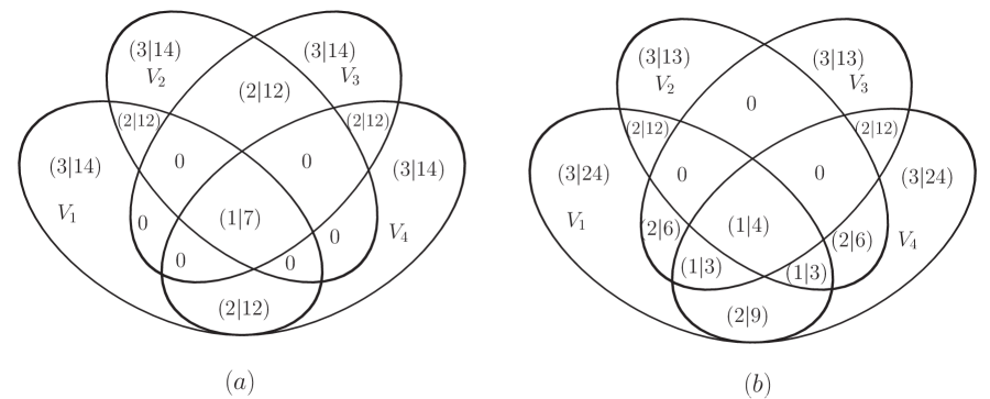
Figure 9: Venn diagrams for intersections of four branches, where each ellipse represents one branch. Venn diagram (a) is for $\mbox{B22}_{(K_{3},K_{4})}^{(m,m)}$, and Venn diagram (b) is for $\mbox{B22}_{(K_{3}/K_{4},\oslash)}^{(m,M)}$, $\mbox{B22}_{(K_{3}/K_{4},\oslash)}^{(M,m)}$. Number 0 means that there is no intersection and $(d|n)$ represents that the dimension of that intersection is $d$ and the number of coefficients detected in that intersection is $n$.

Variety with six branches: For kinematic configuration

$$\mbox{B22}_{(K_{3}/K_{4},\oslash)}^{(m,m)}~{},~{}~{}~{}$$ (119)

the variety is given by six branches $V_{1},V_{2},V_{3},V_{4},V_{5},V_{6}$. Among these six branches, four $V_{i},i=1,2,3,4$ can detect 29 coefficients and the other two $V_{5},V_{6}$ can detect 45 coefficients. All six branches intersect at a single point, and intersection of every five branches is also the same single point. For intersections of every four branches, most of them are the same single point inherit from intersections of every five branches except for the following two combinations of branches $(V_{1},V_{3},V_{5},V_{6})$ and $(V_{2},V_{4},V_{5},V_{6})$, which intersect at 1-dimensional variety detecting $4$ coefficients. For intersections of every three branches, besides the ones that are inherited from intersections of four branches, there are also four pairs $(V_{1},V_{2},V_{5})$, $(V_{1},V_{2},V_{6})$ and $(V_{3},V_{4},V_{5})$, $(V_{3},V_{4},V_{6})$ that intersect at one-dimensional variety detecting 4 coefficients. Intersections of every two branches could be 2-dimensional, 1-dimensional, or single point, and they are summarized as

$$(2|13) = V_{1}\cap V_{2}=V_{1}\cap V_{5}=V_{2}\cap V_{6}=V_{3}\cap V_{4}=V_{3}\cap V_{6}=V_{4}\cap V_{5}~{},~{}~{}~{}$$

$$(2|10) = V_{2}\cap V_{5}=V_{1}\cap V_{6}=V_{4}\cap V_{6}=V_{3}\cap V_{5}~{},~{}~{}~{}$$

$$(1|4) = V_{1}\cap V_{3}=V_{2}\cap V_{4}~{}~{},~{}~{}(0|1)=V_{1}\cap V_{4}=V_{2}\cap V_{3}~{}~{},~{}~{}(1_{2}|7)=V_{5}\cap V_{6}~{}.~{}~{}~{}$$ (120)

One interesting point is that intersection of $(V_{5},V_{6})$ is two 1-dimensional varieties, and to emphasize this subtlety we have used $(1_{2})$ notation.

7.7 The topology (B21): planar triangle-bubble

For this topology we could have two cases $\mbox{B21}_{(K_{2},K_{3})}$ and $\mbox{B21}_{(K_{2}/K_{3},\oslash)}$. For $\mbox{B21}_{(K_{2},K_{3})}$, since there are three external momenta, we can use $K_{1},K_{3}$ to construct momentum basis. For $\mbox{B21}_{(K_{2}/K_{3},\oslash)}$, there are only two external legs, and only one of them is independent. So we need another auxiliary momentum together with $K_{1}$ to construct momentum basis. We do not consider $\mbox{B21}_{(\oslash,\oslash)}$ since it requires $K_{1}=0$, which is tadpole-like structure. For $\mbox{B21}_{(K_{2}/K_{3},\oslash)}$ we also assume that both external momenta are massive for non-vanishing result and do not consider the kinematic configurations where any momentum is massless.

From four propagators we can reduce 8 variables to 7 ISPs, for example, $(x_{2},x_{3},x_{4},y_{1},y_{2},y_{3},y_{4})$. Using Gröbner basis that generated from the three quadratic equations with ordering $(y_{1},x_{2},y_{2},x_{3},y_{3},x_{4},y_{4})$, under the renormalization conditions for monomials

$$\sum_{\mbox{\tiny{all~{}ISPs~{}of~{}x}}}d(x_{i})\leq 3~{},~{}\sum_{\mbox{\tiny{all~{}ISPs~{}of~{}y}}}d(y_{i})\leq 2~{},~{}\sum_{\mbox{\tiny{all~{}ISPs~{}of~{}x}}}d(x_{i})+\sum_{\mbox{\tiny{all~{}ISPs~{}of~{}y}}}d(y_{i})\leq 3~{},~{}~{}~{}$$ (121)

we can get integrand basis for different kinematic configurations. The elements of integrand basis depends on the kinematics of $K_{1}$. For $\mbox{B21}_{(K_{2},K_{3})}$ and $\mbox{B21}_{(K_{2}/K_{3},\oslash)}$, if $K_{1}$ is massive, the integrand basis contains 80 elements given by

$${\cal B}_{B21}^{I} = \{1,x_{2},x_{3},x_{2}x_{3},x_{3}^{2},x_{2}x_{3}^{2},x_{3}^{3},x_{4},x_{2}x_{4},x_{3}x_{4},x_{2}x_{3}x_{4},x_{3}^{2}x_{4},x_{4}^{2},x_{2}x_{4}^{2},x_{3}x_{4}^{2},x_{4}^{3},y_{1},$$ (122)

$$x_{3}y_{1},x_{3}^{2}y_{1},x_{4}y_{1},x_{4}^{2}y_{1},y_{1}^{2},x_{3}y_{1}^{2},x_{4}y_{1}^{2},y_{2},x_{2}y_{2},x_{3}y_{2},x_{2}x_{3}y_{2},x_{3}^{2}y_{2},x_{4}y_{2},x_{2}x_{4}y_{2},$$

$$x_{3}x_{4}y_{2},x_{4}^{2}y_{2},y_{2}^{2},x_{3}y_{2}^{2},x_{4}y_{2}^{2},y_{3},x_{2}y_{3},x_{3}y_{3},x_{2}x_{3}y_{3},x_{3}^{2}y_{3},x_{4}y_{3},x_{2}x_{4}y_{3},x_{3}x_{4}y_{3},$$

$$x_{4}^{2}y_{3},y_{1}y_{3},x_{3}y_{1}y_{3},x_{4}y_{1}y_{3},y_{2}y_{3},x_{2}y_{2}y_{3},x_{3}y_{2}y_{3},x_{4}y_{2}y_{3},y_{3}^{2},x_{2}y_{3}^{2},x_{3}y_{3}^{2},x_{4}y_{3}^{2},y_{4},$$

$$x_{2}y_{4},x_{3}y_{4},x_{2}x_{3}y_{4},x_{3}^{2}y_{4},x_{4}y_{4},x_{2}x_{4}y_{4},x_{3}x_{4}y_{4},x_{4}^{2}y_{4},y_{1}y_{4},x_{3}y_{1}y_{4},x_{4}y_{1}y_{4},y_{2}y_{4},$$

$$x_{2}y_{2}y_{4},x_{3}y_{2}y_{4},x_{4}y_{2}y_{4},y_{3}y_{4},x_{2}y_{3}y_{4},x_{3}y_{3}y_{4},x_{4}y_{3}y_{4},y_{4}^{2},x_{2}y_{4}^{2},x_{3}y_{4}^{2},x_{4}y_{4}^{2}\}~{}.~{}~{}~{}$$

If $K_{1}$ is massless for $\mbox{B21}_{(K_{2},K_{3})}$, integrand basis is given by replacing 8 elements from ${\cal B}_{B21}^{I}$

$${\cal B}_{B21}^{II} = {\cal B}_{B21}^{I}-\{x_{3}x_{4},x_{2}x_{3}x_{4},x_{3}^{2}x_{4},x_{3}x_{4}^{2},x_{3}x_{4}y_{2},x_{3}x_{4}y_{3},x_{3}x_{4}y_{4},x_{2}\ y_{3}y_{4}\}$$ (123)

$$+\{x_{2}^{2},x_{2}^{3},x_{2}^{2}x_{3},x_{2}^{2}x_{4},x_{2}^{2}y_{2},x_{2}y_{2}^{2},x_{2}^{2}y_{3},x_{2}^{2}y_{4}\}~{}.~{}~{}~{}$$

The variety defined by the three quadratic equations is irreducible with dimension four for $\mbox{B21}_{(K_{2},K_{3})}$ with $K_{1}$ massive. If $K_{1}$ is massless, the variety will split into two branches, and each branch can detect 54 coefficients. Intersection of these two branches is an irreducible 3-dimensional variety, and it can detect 28 coefficients. So using both branches, we can detect $54+54-28=80$ coefficients. For $\mbox{B21}_{(K_{2}/K_{3},\oslash)}$, $K_{1}$ should be massive, and the variety has two branches. Each branch can detect 64 coefficients, and intersection of these two branches is an irreducible 3-dimensional variety, which can detect 48 coefficients. Using these two branches we can detect $64+64-48=80$ coefficients of integrand basis.

7.8 The topology (B11): planar sun-set

For this topology, since $K_{1}=-K_{2}$, we use $K_{1}$ and another auxiliary momentum to construct momentum basis. The only possible kinematic configuration is both $K_{1},K_{2}$ massive. There are only three propagators and we can not construct linear equation from on-shell equations, thus there are 8 ISPs. The three quadratic equations can be expressed as

$$D_{0} = x_{1}x_{2}+x_{3}x_{4}~{},~{}\widetilde{D}_{0}=y_{1}y_{2}+y_{3}y_{4}~{},~{}~{}~{}$$

$$\widehat{D}_{0} = x_{2}y_{1}+x_{1}y_{2}+x_{4}y_{3}+x_{3}y_{4}+(x_{1}+y_{1}){\alpha}_{11}+(x_{2}+y_{2}){\alpha}_{12}+{\alpha}_{11}{\alpha}_{12}~{}.~{}~{}~{}$$ (124)

Using Gröbner basis with ordering $(y_{4},y_{3},x_{4},x_{3},y_{2},y_{1},x_{2},x_{1})$, under the renormalization conditions for monomials

$$\sum_{\mbox{\tiny{all~{}ISPs~{}of~{}x}}}d(x_{i})\leq 2~{},~{}\sum_{\mbox{\tiny{all~{}ISPs~{}of~{}y}}}d(y_{i})\leq 2~{},~{}\sum_{\mbox{\tiny{all~{}ISPs~{}of~{}x}}}d(x_{i})+\sum_{\mbox{\tiny{all~{}ISPs~{}of~{}y}}}d(y_{i})\leq 2~{},~{}~{}~{}$$ (125)

we can get 42 elements for integrand basis as

$${\cal B}_{B11} = \{1,x_{1},x_{1}^{2},x_{2},x_{1}x_{2},x_{2}^{2},x_{3},x_{1}x_{3},x_{2}x_{3},x_{3}^{2},x_{4},x_{1}x_{4},x_{2}x_{4},x_{4}^{2},y_{1},x_{1}y_{1},x_{2}y_{1},$$ (126)

$$x_{3}y_{1},x_{4}y_{1},y_{1}^{2},y_{2},x_{1}y_{2},x_{2}y_{2},x_{3}y_{2},x_{4}y_{2},y_{1}y_{2},y_{2}^{2},y_{3},x_{1}y_{3},x_{2}y_{3},x_{3}y_{3},x_{4}y_{3},$$

$$y_{1}y_{3},y_{2}y_{3},y_{3}^{2},y_{4},x_{1}y_{4},x_{2}y_{4},x_{4}y_{4},y_{1}y_{4},y_{2}y_{4},y_{4}^{2}\}~{}.~{}~{}~{}$$

The variety defined by the three quadratic equations is irreducible with dimension five.

8 Conclusion

In this paper, we use the new technique developed in [27, 28, 29] to classify the two-loop integrand basis in pure four dimension space-time. Although there are only small number of topologies for planar and non-planar two-loop diagrams, the diverse external momentum configurations greatly increase the number of integrand basis that we need to discuss. Because the integrand basis and branch structure of variety will depend on the topology as well as external kinematics, it is necessary to classify possible sets of integrand basis and study the evolution of variety under various kinematic limits.

The algebraic geometry methods, such as Gröbner basis method and multivariate polynomial division, play a crucial role in our discussion. Using these methods, we are able to present explicit form of integrand basis as well as detailed study of varieties, such as branch structures and their intersections. The same methods also allow us to determine coefficients of integrand basis.

We must emphasize that our result is only a small step towards the practical evaluation of general two-loop amplitudes. As we have mentioned in the introduction, the number of two-loop integrand basis is much more than the number of two-loop integral basis and it is highly desirable to reduce integrand basis further. One way to do so is to use the IBP-method [18]. However, with the time consuming, it is not feasible at this moment.

Although our results are for two-loop diagrams in pure four-dimension space-time, the same analysis can be applied to $(4-2\epsilon)$-dimension for complete answer, or three and higher loop amplitudes as demonstrated in [29]. It is also an interesting problem to apply these general analysis to real processes.

Appendix A Some mathematical backgrounds

In this section, we present several mathematical facts that may be useful for determining branch structure of non-linear on-shell equations. First let us consider the quadratic equation of two variables defined by equation

$$Ax^{2}+Bxy+Cy^{2}+Dx+Ey+F=0~{},~{}~{}~{}$$ (127)

with $A,B,C$ not all zero. This equation is usually called conic section. In general, the conic is an irreducible one-dimensional variety, however, when the determinant $\Delta$ of following $3\times 3$ matrix

$$\Delta={\rm det}\left(\begin{array}[]{ccc}A&B/2&D/2\\ B/2&C&E/2\\ D/2&E/2&F\\ \end{array}\right)={-(B^{2}-4AC)F+BDE-CD^{2}-AE^{2}\over 4}~{}~{}~{}~{}$$ (131)

is zero, the conic splits to two branches.

Next let us consider the roots of a polynomial

$$f(z)=\sum_{i=0}^{n}a_{i}z^{i}~{}.~{}~{}~{}$$ (132)

One can use discriminant to determine whether if this polynomial has repeated roots or not. If discriminant equals to zero, then there are repeated roots. The simplest example is quadratic equation $a_{2}z^{2}+a_{1}z+a_{0}=0$ whose discriminant is $D=a_{1}^{2}-4a_{0}a_{2}$. If $D=0$, then this equation has double roots, and the polynomial can be written as a perfect square of one factor. The discriminant of $n=2,3$ can be found in many other references, and using it we can tell the properties of roots just from coefficients of variable. A special interesting example is the quartic function

$$f(z)=Az^{4}+Bz^{3}+Cz^{2}+Dz+E~{},~{}~{}~{}$$ (133)

which can be factorized as

$$f(z)\sim(z-z^{(+,+)})(z-z^{(+,-)})(z-z^{(-,+)})(z-z^{(-,+)})~{},~{}~{}~{}$$ (134)

where $z^{\pm,\pm}$ are four roots. We want to know if it can be expressed as perfect square terms such as

$$f(z)=(az+b)^{2}(cz+d)^{2}~{}.~{}~{}~{}$$ (135)

In other words, we want to know if there are repeated roots or not. Defining

$$\mathcal{A}=-{3B^{2}\over 8A^{2}}+{C\over A}~{}~{},~{}~{}\mathcal{B}={B^{3}\over 8A^{3}}-{BC\over 2A^{2}}+{D\over A}~{}~{},~{}~{}\mathcal{C}=-{3B^{4}\over 256A^{4}}+{CB^{2}\over 16A^{3}}-{BD\over 4A^{2}}+{E\over A}~{},~{}~{}~{}$$ (136)

then when $\mathcal{B}=0$, the quartic equation has following solution

$$z=-{B\over 4A}\pm_{s}\sqrt{{-\mathcal{A}\pm_{t}\sqrt{\mathcal{A}^{2}-4\mathcal{C}}\over 2}}~{},~{}~{}~{}$$ (137)

where $\pm_{s}$ and $\pm_{t}$ can take plus and minus sign independently. If the coefficients further satisfy $\mathcal{A}^{2}-4\mathcal{C}=0$, then $x^{(s,+)}=x^{(s,-)}$, and $f(x)$ can be expressed as products of two perfect squares.

Using above results, we can check whether variety defined by following equations is reducible

$$Ax^{2}+Bxy+Cy^{2}+Dx+Ey+F=0~{},~{}~{}~{}$$ (138)

$$a(\tau)x+b(\tau)y+c(\tau)=0~{},~{}~{}~{}$$ (139)

where $a(\tau),b(\tau),c(\tau)$ are linear functions of (possible free parameter) $\tau$. After solving the linear equation of $x,y$ and substituting the result into quadratic equation we get

$$(a^{2}C-abB+b^{2}A)y^{2}+(a^{2}E-abD-acB+2bcA)y+(a^{2}F-acD+c^{2}A)=0~{},~{}~{}~{}$$ (140)

where the coefficients $A^{\prime}(\tau)=(a^{2}C-abB+b^{2}A)$, $B^{\prime}(\tau)=(a^{2}E-abD-acB+2bcA)$ and $C^{\prime}(\tau)=(a^{2}F-acD+c^{2}A)$ are now quadratic functions of $\tau$. The solution of $y$ is given by

$$y={-B^{\prime}(\tau)\pm\sqrt{B^{\prime}(\tau)^{2}-4A^{\prime}(\tau)C^{\prime}(\tau)}\over 2A^{\prime}(\tau)}~{},~{}~{}~{}$$ (141)

thus $y$ is a rational function of $\tau$ when and only when terms inside the square root is perfect square, i.e., the quartic function $(B^{\prime}(\tau)^{2}-4A^{\prime}(\tau)C^{\prime}(\tau))$ of $\tau$ is a perfect square.

References

- [1] J. Alcaraz Maestre et al. [SM AND NLO MULTILEG and SM MC Working Groups Collaboration], arXiv:1203.6803 [hep-ph].
- [2] J. R. Andersen et al. [SM and NLO Multileg Working Group Collaboration], arXiv:1003.1241 [hep-ph].
- [3] G. Passarino and M. J. G. Veltman, “One Loop Corrections For E+ E- Annihilation Into Mu+ Mu- In The Weinberg Model,” Nucl. Phys. B 160, 151 (1979).
- [4] L. D. Landau, Nucl. Phys. 13, 181 (1959); S. Mandelstam, Phys. Rev. 112, 1344 (1958); S. Mandelstam, Phys. Rev. 115, 1741 (1959); R. E. Cutkosky, J. Math. Phys. 1, 429 (1960).
- [5] Z. Bern, L. J. Dixon, D. C. Dunbar and D. A. Kosower, Nucl. Phys. B 435, 59 (1995) [hep-ph/9409265].
- [6] Z. Bern, L. J. Dixon, D. C. Dunbar and D. A. Kosower, Nucl. Phys. B 425, 217 (1994) [hep-ph/9403226].
- [7] C. Anastasiou, R. Britto, B. Feng, Z. Kunszt and P. Mastrolia, Phys. Lett. B 645, 213 (2007) [hep-ph/0609191].
- [8] C. Anastasiou, R. Britto, B. Feng, Z. Kunszt and P. Mastrolia, JHEP 0703, 111 (2007) [hep-ph/0612277].
- [9] R. Britto, F. Cachazo and B. Feng, Nucl. Phys. B 725, 275 (2005) [hep-th/0412103].
- [10] R. Britto, E. Buchbinder, F. Cachazo and B. Feng, Phys. Rev. D 72, 065012 (2005) [hep-ph/0503132].
- [11] G. Ossola, C. G. Papadopoulos and R. Pittau, Nucl. Phys. B 763, 147 (2007) [hep-ph/0609007].
- [12] D. Forde, Phys. Rev. D 75, 125019 (2007) [arXiv:0704.1835 [hep-ph]].
- [13] R. K. Ellis, W. T. Giele and Z. Kunszt, JHEP 0803, 003 (2008) [arXiv:0708.2398 [hep-ph]].
- [14] W. B. Kilgore, arXiv:0711.5015 [hep-ph].
- [15] W. T. Giele, Z. Kunszt and K. Melnikov, JHEP 0804, 049 (2008) [arXiv:0801.2237 [hep-ph]].
- [16] G. Ossola, C. G. Papadopoulos and R. Pittau, JHEP 0805, 004 (2008) [arXiv:0802.1876 [hep-ph]].
- [17] S. D. Badger, JHEP 0901, 049 (2009) [arXiv:0806.4600 [hep-ph]].
-
[18]
F. V. Tkachov, Phys. Lett. B 100, 65 (1981);
K. G. Chetyrkin and F. V. Tkachov, Nucl. Phys. B 192, 159 (1981).
S. Laporta, Phys. Lett. B 504, 188 (2001) [hep-ph/0102032].
S. Laporta, Int. J. Mod. Phys. A 15, 5087 (2000) [hep-ph/0102033]. - [19] P. Mastrolia and G. Ossola, JHEP 1111, 014 (2011) [arXiv:1107.6041 [hep-ph]].
- [20] S. Badger, H. Frellesvig and Y. Zhang, JHEP 1204, 055 (2012) [arXiv:1202.2019 [hep-ph]].
- [21] J. Gluza, K. Kajda and D. A. Kosower, Phys. Rev. D 83, 045012 (2011) [arXiv:1009.0472 [hep-th]].
- [22] D. A. Kosower and K. J. Larsen, Phys. Rev. D 85, 045017 (2012) [arXiv:1108.1180 [hep-th]].
- [23] K. J. Larsen, arXiv:1205.0297 [hep-th].
- [24] S. Caron-Huot and K. J. Larsen, arXiv:1205.0801 [hep-ph].
- [25] R. H. P. Kleiss, I. Malamos, C. G. Papadopoulos and R. Verheyen, arXiv:1206.4180 [hep-ph].
- [26] H. Johansson, D. A. Kosower and K. J. Larsen, arXiv:1208.1754 [hep-th].
- [27] Y. Zhang, arXiv:1205.5707 [hep-ph].
- [28] P. Mastrolia, E. Mirabella, G. Ossola and T. Peraro, arXiv:1205.7087 [hep-ph].
- [29] S. Badger, H. Frellesvig and Y. Zhang, JHEP 1208, 065 (2012) [arXiv:1207.2976 [hep-ph]].
- [30] D. Mehta, Y. -H. He and J. D. Hauenstein, JHEP 1207, 018 (2012) [arXiv:1203.4235 [hep-th]].
- [31] D. R. Grayson and M. E. Stillman, Macaulay2, a software system for research in algebraic geometry. Available at http://www.math.uiuc.edu/Macaulay2/.