Calculation of the melting point of alkali halides by means of computer simulations

Abstract

In this manuscript we study the liquid-solid coexistence of NaCl-type alkali halides, described by interaction potentials such as Tosi-Fumi (TF), Smith-Dang (SD) and Joung-Cheatham (JC), and compute their melting temperature (T_m) at 1 bar via three independent routes: 1) liquid/solid direct coexistence, 2) free-energy calculations and 3) Hamiltonian Gibbs-Duhem integration. The melting points obtained by the three routes are consistent with each other. The calculated T_m of the Tosi-Fumi model of NaCl is in good agreement with the experimental value as well as with other numerical calculations. However, the other two models considered for NaCl, SD and JC, overestimate the melting temperature of NaCl by more than 200 K. We have also computed the melting temperature of other alkali halides using the Tosi-Fumi interaction potential and observed that the predictions are not always as close to the experimental values as they are for NaCl. It seems that there is still room for improvement in the area of force-fields for alkaline halides, given that so far most models are still unable to describe a simple yet important property such as the melting point.

I Introduction

Alkali halides are inorganic compounds composed of an alkali metal and a halogen. The most abundant by far in Nature is Sodium Chloride (NaCl). NaCl in its solid form has a cubic structure (usually denoted as NaCl structure) and melts at a relatively high temperature (around 1070 K at ambient pressure) as a consequence of its high lattice energy. NaCl dissolves in polar solvents, such as water, to give ionic solutions that contain highly solvated anions and cations, relevant for the functioning of biological organisms.

In the last century, there have been many thorough studies aimed at quantitatively describing the physical properties of alkali halides. To a first approximation alkali halides are two-component mixtures of atomic anions and cations which interact through a spherically symmetrical potential. The two unusual features of ionic crystals are the slow decay of the interaction potential, which causes long-range structural correlations, and the strength of the attractive cation-anion interactions. The simplest model for a molten salt is the restricted primitive model (RPM) , in which ions are modelled by hard spheres with positive and negative unit charges. The RPM has been studied by a number of groupsGroth et al. (1998); Orkoulas and Panagiotopoulos (1999); Ciach and Stell (2004); Hynninen et al. (2006); Gonzalez-Melchor et al. (2003); Vega et al. (1996, 2003). Back in 1919, Born developed a numerical model to estimate the energy of an ionic crystal Born and Verh (1919). Pauling, based on Born’s primitive model, studied the effect of the ions’ sizes on ionic salts Pauling (1928a, b) and Mayer evaluated the role of polarizability and dispersive forces on alkali halides Mayer (1933) and proposed, together with Huggins, a generalization of Born’s repulsive energy Huggins and Mayer (1933). More recently, several ion-ion interaction potentials have been developed in order to numerically simulate alkali halides. In 1962 Tosi and Fumi, fitting the Huggins-Mayer dispersive energy to crystallographic data, proposed an empirical potential parameterizing the repulsive part of the NaCl alkali halide interactions Fumi and Tosi (1964) and including the dipole-quadrupole van der Waals term, that imitated the polarization distortion of the electronic cloud. The advantages and disadvantages of the Tosi-Fumi (TF) potential have been later underlined by Lewis and coworkers Lewis et al. (1975). The model in general predicts good densities and lattice energies of alkaline halides. However it is unable to reproduce dynamical features of ionic crystals such as the phonon dispersion curves. Also the model predicts incorrectly the similarity of like pair distribution functions $g^{--}$ and $g^{++}$ which is absent in the experiments Wilson and Madden (1992). The TF model was used for the first time in a numerical simulation by Adams and McDonald Adams and McDonald (1974), who obtained a remarkably good agreement between numerical and experimental results. In recent years, the Tosi-Fumi potential has also been used to study liquid/solid phase transitions in alkali halides: Valeriani et al. studied homogeneous crystal nucleation in molten NaCl Valeriani et al. (2005) and Chen and Zhu carried out homogeneous nucleation studies of other alkali halides, such as KBr Chen et al. (2004) and NaBr Zhu (2004). Zykova-Timan et al. studied packing issues related to the interfacial free-energy between the liquid and solid phases Zykova-Timan et al. (2004); T.Zykova-Timan et al. (2008). In all these works knowledge of the melting temperature $T_{m}$ was needed. In fact, the melting point of NaCl has been estimated for the TF model by several groups. In 2003, Anwar et al. determined by free-energy calculations the melting temperature of NaCl for the Tosi-Fumi model Anwar et al. (2003). Later on similar results were obtained by Eike et al. Eike et al. (2005) and Mastny et al. Mastny and de Pablo (2005) and by Zykova-Timan et al. Zykova-Timan et al. (2005). Molecular simulations have also been performed to analyze experimental results Boehler et al. (1997, 1996). In some works the melting temperature was calculated by direct heating of the solid, hence the thermal instability limit rather that the melting temperature was calculated Belonoshko et al. (2000). More recently in order to compute T_m Belonoshko et al. performed two-phase simulations of NaCl and LiF  Belonoshko and Dubrovinsky (1996); Belonoshko et al. (2000).

Besides TF, another popular model used to describe NaCl was proposed more recently by Smith and Dang (SD) Smith and Dang (1994); Dang and Smith (1993) who presented an interaction potential where the ion-ion interactions were Lennard-Jones like. This model potential has become quite popular when studying NaCl in water solutions, even though the properties of its solid phase are still unknown. Similar to the SD potential, Joung-Cheatham (JC) presented another interaction potential for NaCl where the ion-ion interactions were Lennard-Jones like and proposed several NaCl force-fields tailored to be used in a water solution Joung and Cheatham (2008). Somewhat surprisingly the melting point of the SD and JC/NaCl potentials are still unknown.

Good model potentials for alkali halides are also useful to study ionic solutions. Simulations of alkali halides dissolved in water have proved useful to study thermodynamic mixing properties, such as the cryoscopic descent of the melting temperature Vrbka and Jungwirth (2007). The properties of alkali halides solutions have been studied at low temperatures in order to localize the hypothesised second critical point of water Corradini et al. (2010, 2011); Poole et al. (1992). The solubility of NaCl in water has also received certain interest Moucka et al. (2011); Sanz and Vega (2007); Aragones et al. (2012); Joung and Cheatham (2009); Lisal et al. (2005); Paluch et al. (2010); Moucka et al. (2012). However we should underline that in order to determine the solubility of a salt, the chemical potential of the solid should be known.

Thus, it is relevant to quantitatively compare several interaction potentials in order to estimate their efficiency in mimicking the properties of NaCl-type alkali halides. To this aim, in this manuscript we evaluate the liquid-solid equilibrium of such systems. We have computed the melting temperature (at normal pressure) for three alkali halides, emphasizing NaCl, for three interaction models: the Born-Mayer-Huggins-Tosi-Fumi (TF) Mayer (1933); Huggins and Mayer (1933); Fumi and Tosi (1964); Adams and McDonald (1975), the Smith-Dang (SD) Smith and Dang (1994) and the Joung-Cheatham (JC) potential Joung and Cheatham (2008). The three potentials are two-body and non-polarizable model potentials, characterized by a repulsive term, a short-range attraction and a long-range Coulombic interaction term. To calculate the melting temperature (T_m) we used three independent routes: 1) liquid/solid direct coexistence 2) free-energy calculations and 3) Hamiltonian Gibbs-Duhem integration. We have found that the value obtained for the T_m of the TF/NaCl is in good agreement with the experiment, in contrast with the results obtained for the SD/NaCl and JC/NaCl models. Therefore, we conclude that the TF/NaCl model is the most suitable for studies of pure NaCl. Using Hamiltonian Gibbs-Duhem integration we have also evaluated T_m for other TF/alkali halides and concluded that the quality of the results obtained with the TF potential depends on the alkali halide chosen. The TF model provides good predictions for alkali halides that involve K⁺, Cl^-, Na⁺, Br^- and Li⁺ ions, whereas it performs much worse for alkali halides involving Rb⁺ or F^- ions.

The manuscript is organized as follows: we first introduce the interaction potentials of the alkali halides under study, i.e. Born-Mayer-Huggins-Tosi-Fumi potential (TF), the Smith-Dang potential (SD) and the Joung-Cheatham (JC) potential. Then we describe the three simulation routes followed to compute their melting temperature: 1) the liquid/solid direct coexistence 2) the Einstein crystal/molecule for the solid and the thermodynamic integration for the liquid and 3) the Hamiltonian Gibbs-Duhem integration. To conclude we will present our results obtained for different alkali halides.

II Simulation methods

The interaction potentials we used are two-body and non-polarizable model potentials, each of them characterized by a repulsive term, a short-range attractive and a long-range Coulomb interaction term. The TF model potential has the following form:

$$U(r_{ij})=A_{ij}e^{-r_{ij}/\rho_{ij}}-\frac{C_{ij}}{r_{ij}^{6}}-\frac{D_{ij}}{r_{ij}^{8}}+\frac{q_{i}q_{j}}{4\pi\epsilon_{o}r_{ij}}$$ (1)

where $r_{ij}$ is the distance between two ions with charge $q_{i,j}$, the first term is the Born-Mayer repulsive term, $-\frac{C_{ij}}{r_{ij}^{6}}$ and $-\frac{D_{ij}}{r_{ij}^{8}}$ are the Van der Waals attractive interaction terms and the last term corresponds to the Coulomb interaction. The parameters $A_{ij}$, $\rho_{ij}$, $C_{ij}$ and $D_{ij}$ for the TF/alkali halides are given as Supplementary Materialmat .

Both the SD and the JC model potentials can be written using the following expression:

$$U(r_{ij})=4\epsilon\left[\left(\frac{\sigma_{ij}}{r_{ij}}\right)^{12}-\left(\frac{\sigma_{ij}}{r_{ij}}\right)^{6}\right]+\frac{q_{i}q_{j}}{4\pi\epsilon_{o}r_{ij}}$$ (2)

where $r_{ij}$ is the distance between two ions with charge $q_{i,j}$. The first term is Lennard-Jones-like, and its parameters are given in the Supplementary Information filemat . The last term in Eq. 2 corresponds to the Coulomb interaction. For the JC potential, we are going to use the parameters introduced to simulate NaCl in SPC/E water Joung and Cheatham (2008).

For the SD and JC the crossed interaction parameters are obtained using the Lorentz-Berthelot combining rules Lorentz (1881); Berthelot (1898). It is interesting to point out that the TF model was developed to study ionic crystals and pure alkali halides in the solid phase whereas the SD was obtained to model Na⁺ and Cl^- in water. The JC was fitted to model NaCl both in the solid phase and in aqueous solutions. In what follows, we shall refer to ions as particles.

When computing T_m for the TF/NaCl interaction potential, we follow three independent routes: 1) liquid/solid direct coexistence, 2) free-energy calculations and 3)Hamiltonian Gibbs-Duhem integration. For the SD/NaCl and JC/NaCl and for other TF/alkali halides we use the first and the third route.

II.1 Route 1. Liquid/solid direct coexistence

The first route we follow to compute the melting temperature is by means of the liquid/solid direct coexistence, originally proposed in Ref. Ladd and Woodcock (1977, 1978); Morris and Song (2002); Yoo et al. (2004); Karim and Haymet (1988). To start with, we generate an equilibrated configuration of the NaCl solid phase in contact with its liquid. After having prepared the liquid-solid configuration, we run several NpT simulations (with anisotropic scaling, so that each side of the simulation box changes independtly) at different temperatures and always at a pressure of 1 bar. Direct coexistence simulations should be performed in the Np_zT ensemble, where z is the axis perpendicular to the fluid-solid interface and $x$ and $y$ have been chosen carefully to avoid the presence of stress. However, we have recently shown that NpT simulations (with anisotropic scaling) provide proper results for sufficiently large systems Noya et al. (2008a); Fernandez et al. (2006). Depending on the temperature, the system evolves towards complete freezing or melting of the sample. Since we do not know the location of the melting temperature, we simulate the system in a wide range of temperatures and identify the melting temperature $T_{m}$ as the average of the highest temperature at which the liquid freezes and the lowest temperature at which the solid melts. A more elaborate procedure would require to estimate the slope of the growth rate of the solid-fluid interface ( which is positive at temperatures below the melting point and negative at temperatures above the melting point) and to locate the temperature at which the growth rate of interface is zero (i.e the melting point). Since the growth of the solid is a stochastic process the determination of the growth rate requires to accumulate statistics over many different trajectories making the calculations quite expensiveRozmanov and Kusalik (2011); Weiss et al. (2011). The procedure used here is simpler and has provided reliable results for other systems as hard spheresNoya et al. (2008a); Fernandez et al. (2006) or waterFernandez et al. (2006) although admittedly it yields a somewhat larger error in the estimate of the melting point temperature obtained from direct coexistence simulations (of about 5K).

II.2 Route 2. Free-energy calculations

In this route, we first compute the Helmholtz free-energy of both the solid and the liquid phase; next, we estimate the Gibbs free-energy ($G$) by simply adding $pV$. To compute the melting temperature we perform thermodynamic integration as a function of temperature at constant pressure to evaluate where the chemical potentials ($\mu=G/N$) of both phases coincides. To estimate the free-energy of the bulk solid phase we use the Einstein crystal Frenkel and Ladd (1984) and the Einstein molecule methods Vega and Noya (2007); Noya et al. (2008b). Both methods are based on the calculation of the free-energy difference between the target solid and a reference system at the solid equilibrium-density for the given thermodynamic conditions (obtained with an NpT simulation). The reference system of the Einstein crystal method consists of an ideal solid whose free-energy can be analytically computed (an “Einstein crystal” with the center of mass fixed, where the inter-molecular interactions are neglected and particles are bound to their lattice equilibrium positions by a harmonic potential with strength $\Lambda_{E}$). The Einstein molecule method differs from the previous one due to the fact that we now fix only the position of one particle instead of the center of mass.

Thermodynamic integration is performed in two steps Vega et al. (2008): 1) we evaluate the free-energy difference ($\Delta$ A₁) between the ideal Einstein crystal and the Einstein crystal in which particles interact through the Hamiltonian of the original solid (“interacting” Einstein crystal). 2) Next we calculate the free-energy difference ($\Delta$ A₂) between the interacting Einstein crystal and the original solid, by means of thermodynamic integration: $U(\lambda)=\lambda U_{sol}+(1-\lambda)(U_{Ein-id}+U_{sol})$), where $U_{Ein-id}$ represents the energy of the interacting Einstein crystal, $U_{sol}$ the one of the original solid, and $\lambda$ is the coupling parameter that allows us to integrate from the interacting Einstein crystal ($\lambda=0$) to the desired solid ($\lambda=1$). The final expression of the Helmholtz free-energy $A^{NaCl}_{sol}(T,V)$ coming from the Einstein crystal/molecule calculations is Vega et al. (2008):

$$A_{sol}^{NaCl}(T,V)=A_{0}(T,V)+\Delta A_{1}(T,V)+\Delta A_{2}(T,V)$$ (3)

where A₀ is the free energy of the reference system, whose analytical expression is slightly different in the Einstein crystal and Einstein molecule (see Ref. Vega et al. (2008)). $\Delta$A₁ and $\Delta$A₂ are computed in the same way in the Einstein crystal and Einstein molecule methods (the only difference being the choice of the point that remains fixed in the simulations, whether the system’s center of mass or a reference particle’s center of mass). It has been shown that, since the free energy of a solid is uniquely defined, its value does not depend on the method used to compute it and the two methodologies give exactly the same results Vega et al. (2008). It is convenient to set the thermal De Broglie wave length of all species to 1 Å, and the internal partition functions of all species to one. These arbitrary choices affect the value of the free energy but does not affect phase equilibria (provided the same choice is adopted in all phases).

To estimate the free-energy of the bulk liquid we use Hamiltonian thermodynamic integration as in Ref. Anwar et al. (2003), calculating the free-energy difference between the liquid alkali halide and a reference Lennard-Jones (LJ) liquid for which the free-energy is known. Starting from an equilibrated NaCl liquid, we perturb the Hamiltonian of the system so that each ion is gradually transformed into a LJ atom. The path connecting both states is given by:

$$U(\lambda)=\lambda U^{LJ}+(1-\lambda)U^{NaCl}$$ (4)

where $U^{LJ}$/$U^{NaCl}$ are the total energies of the Lennard Jones and NaCl fluids, respectively, and $\lambda$ is the coupling parameter ($\lambda=0$ corresponds to NaCl whereas $\lambda$=1 to a LJ fluid). The Helmholtz free-energy of a NaCl (A${}^{NaCl}_{liq}$) is computed as:

$$A_{liq}^{LJ}(T,V) = A_{liq}^{NaCl}(T,V)+\int_{\lambda=0}^{\lambda=1}\langle U^{LJ}-U^{NaCl}\rangle_{N,V,T,\lambda}d\lambda$$ (5)

$$= A_{liq}^{NaCl}(T,V)+\Delta A_{liq}^{LJ}(T,V)$$

Given that the Lennard-Jones free-energy (A${}_{liq}^{LJ}$) is already known Kolafa and Nezbeda (1994) and the integral in the Eq. 5 ($\Delta A_{liq}^{LJ}$) can be numerically evaluated, we can determine the free-energy A${}^{NaCl}_{liq}$ of the liquid alkali halide. In order to estimate the integral in Eq. 5, we choose 20 values of $\lambda$ between 0 and 1, 10 of them equally spaced from 0.000 to 0.95 and the remaining 10 from 0.95 to 1.000, and integrate each region using the Simpson integration method. This choice originated from then fact that when $\lambda$ has a value close to 1.0, the integrand changes abruptly, dropping to the dispersive energy of a LJ. The Lennard-Jones free-energy consists of two terms: $A_{liq}^{LJ}(T,V)=A_{liq}^{LJ,id}(T,V)+A_{liq}^{LJ,res}(T,V)$, where A${}_{liq}^{LJ,res}(T,V)$ is the excess and A${}_{liq}^{LJ,id}(T,V)$ the ideal part. A${}_{liq}^{LJ,res}$ for a Lennard-Jones fluid has been already computed for a broad range of temperatures and densities in Ref. Johnson et al. (1993); Kolafa and Nezbeda (1994). The free energy of the ideal gas of a mixture of N_Na and N_Cl is given by

$$\frac{1}{k_{B}T}A_{liq}^{LJ,id}(T,V) = N_{Na}ln(\rho_{Na}\Lambda^{3}_{{Na}})-N_{Na}$$ (6)

$$+ N_{Cl}ln(\rho_{Cl}\Lambda^{3}_{Cl})-N_{Cl}$$

$$= N[ln(\rho/2)-1]$$

where N = N_Na+ N_Cl is the total number of particles in the system with density $\rho=\frac{N}{V}$ (and $\rho_{Na}=\frac{N_{Na}}{V}$ = $\rho_{Cl}=\frac{N_{Cl}}{V}$ = $\rho$/2) and $\Lambda_{i}$ is the De Broglie thermal length ($\Lambda$_i = h / $\sqrt{2\pi m_{i}k_{B}T}$), that we arbitrarily set to 1 Å, to be consistent with our choice for the solid phase.

II.3 Route 3. Hamiltonian Gibbs-Duhem integration

The third route we follow to compute the melting temperature is by means of Hamiltonian Gibbs-Duhem thermodynamic integration as in Ref. Agrawal and Kofke (1995a, b); Vega et al. (2005). Starting from the liquid-solid coexistence point of a reference system ($A$), the Hamiltonian Gibbs-Duhem thermodynamic integration allows one to compute the coexistence point of the system of interest (whose Hamiltonian is $B$) by resolving a Clapeyron-like differential equation. In more detail, the Hamiltonian of the initial system (with energy $U_{A}$), whose two-phases coexistence point is known, is connected to the one of the final system of interest (with energy $U_{B}$), via the following expression:

$$U(\lambda)=\lambda U_{B}+(1-\lambda)U_{A}$$ (7)

where $\lambda$ is the coupling parameter. When two phases coexist (labeled as I and II): $\mu_{I}(T,p,\lambda)=\mu_{II}(T,p,\lambda)$, being $\mu=G/N$ the Gibbs free-energy per particle (the chemical potential of each phase). Therefore, differentiating $\mu$ in both phases, we can write generalized Clapeyron equations for two coexisting phases as

$$v_{I}(T,p)dp-s_{I}(T,p)dT+\left(\frac{\partial\mu_{I}(T,p,\lambda)}{\partial\lambda}\right)d\lambda=$$

$$=v_{II}(T,p)dp-s_{II}(T,p)dT+\left(\frac{\partial\mu_{II}(T,p,\lambda)}{\partial\lambda}\right)d\lambda$$ (8)

where $v$ and $s$ are the volume and entropy per particle. If $\lambda$ is constant we recover the well known Clapeyron equation. If the pressure is constant we obtain the slope of the coexistence line in the $\lambda$-T plane:

$$\frac{dT}{d\lambda}=\frac{T[(\partial\mu_{II}/\partial\lambda)-(\partial\mu_{I}/\partial\lambda)]}{h_{II}-h_{I}}=$$

$$=\frac{T[(\partial\mu_{II}/\partial\lambda)-(\partial\mu_{I}/\partial\lambda)]}{\Delta h}$$ (9)

knowing that, at coexistence

$$s_{II}-s_{I}=\frac{h_{II}-h_{I}}{T}.$$ (10)

When a liquid coexists with a solid, ($s_{II}-s_{I}$) is the melting entropy difference $\Delta s_{m}$, that can be easily computed as $\frac{\Delta h_{m}}{T_{m}}$. $\Delta$h is obtained from the NpT simulations at (p,$\lambda$,T) constants, whereas $\frac{\partial\mu}{\partial\lambda}=\langle\frac{\partial u(\lambda)}{\partial\lambda}\rangle_{N,p,T,\lambda}$, computed with an NpT simulation at different values of $\lambda$ in each phase.

Therefore, using Eq. 7, the generalized Clapeyron equation can be written as:

$$\frac{dT}{d\lambda}=\frac{T[\langle u_{B}-u_{A}\rangle^{II}_{N,p,T,\lambda}-\langle u_{B}-u_{A}\rangle^{I}_{N,p,T,\lambda}]}{\Delta h}$$ (11)

where $u_{B}/u_{A}$ is the internal energy per particle when the interaction between particles is described by $U_{B}/U_{A}$. The numerical integration of the generalized Clapeyron equation in Eq. 11 yields the change of the coexistence temperature (at constant pressure) due to the change in the Hamiltonian of the system, starting from the initial coexistence point (where interactions are described by $U_{A}$) to the final coexistence point (where interactions are described by $U_{B}$).

III Simulation Details

When using the liquid/solid direct coexistence route to compute the melting temperature we choose systems containing either 1024 [512 solid/512 liquid], 2000 [1000solid/1000liquid] or 4000 ions [2000 solid/2000 liquid]. When using the free-energy calculations route to compute the melting temperature, we simulate systems of 1000 ions (the unit cell of NaCl contains 8 particles). For the Hamiltonian Gibbs-Duhem integration route we simulate systems of 1000 ions.

We simulated NaCl using the TF, the SD and the JC interaction potentials. For the other alkali halides considered in this work we used only the TF potential. In this work we truncated the non-Coulomb part of the potential at r_c=14 Å  and added tail corrections. We used Ewald sums to deal with Coulombic interactions, truncating the real part of the Ewald sums at the same cut-off as the non-Coulombic interactions and chose the parameters of the Fourier part of the Ewald sums so that $\alpha\cdot r_{c}=2.98$ Frenkel and Smit (2002); Allen and Tildesley (1987). To calculate T_m for the SD and JC models via direct coexistence we performed NpT molecular dynamic simulations (MD) of systems containing 2000 particles with the Gromacs package der Spoel et al. (2005), where we kept the temperature constant with a Nose-Hoover thermostat Nosé (1984); Hoover (1985) with a relaxation time of 2 ps, and the pressure constant at 1 bar with a Parrinello-Rahman barostat Parrinello and Rahman (1981) with a relaxation time of 2 ps. In our MD simulations, we allowed the different box lengths to fluctuate independently. For the TF alkali halides direct coexistence simulations we used NpT Monte Carlo simulations.

In the free-energy calculations, we used the Einstein Crystal and the Einstein Molecule methods to compute the free-energy of the solid phase. We performed an initial equilibration run of the solid in the NpT ensemble of about 10⁵ Monte Carlo (MC) cycles to obtain the equilibrium density at the given thermodynamic conditions. We define a MC cycle as a translational trial-move per particle and a trial-volume change. For the thermodynamic integration in the NVT ensemble we carried out 2x10⁴ equilibration and 8x10⁴ production cycles for every value of $\lambda$ and simulated 20 values of $\lambda$ per thermodynamic state. We also used thermodynamic integration to compute the free-energy of the liquid phase. We carried out 8x10⁴ equilibration and 18x10⁴ production cycles for every value of $\lambda$ and simulated 21 values of $\lambda$ per thermodynamic state. Free-energy calculations were performed at 1083 K and 1 bar. To obtain the equilibrium densities at these thermodynamic conditions, we run NpT MC simulations of the liquid and solid phases. Once equilibrated, we used those densities in the free energy calculations.

When performing the thermodynamic integration to compute the free-energy of the liquid phase (route 2), we tested the dependence of our results on the choice of the reference system by performing the thermodynamic integration to two Lennard-Jones models with different parameters: the parameters set $LJ1$ used by Anwar et al. Anwar et al. (2003) and another set of parameters denoted as $LJ2$. Both sets of parameters are represented in Table 1.

$\epsilon$/kB [LJ1]	$\sigma$	$\rho$*	T*	$\epsilon$/kB [ LJ2]	$\sigma$	$\rho$*	T*
537.01	2.32	0.3766	2.02	358.00	3.00	0.8143	3.03

Table 1: $LJ1$ and $LJ2$ sets of parameter with units $\epsilon$/k_B($[K]$) and $\sigma$([$\AA$]). $\rho$*=$\rho\sigma^{3}$ and T*=$k_{B}$T/$\epsilon$.

The values of $\rho$* and T* shown in Table 1 are obtained by scaling the density and temperature of the liquid phase of the TF/NaCl at 1083 K and 1 bar to LJ reduced units. The free-energy should be independent of the choice of the LJ reference system. Notice that the free-energy of the LJ system given by the Nezbeda equation of state (EOS)  Kolafa and Nezbeda (1994) has a lower error when using LJ2 (at $\rho$*=0.8143 and T*=3.03) rather than at $\rho$*=0.3766 and T*=2.02 (when using LJ1) due to the proximity of the LJ fluid critical point.

When using the third route to compute the melting temperature, we integrated the Hamiltonian in Eq. 7 from the TF/NaCl to the SD and JC potentials and from the TF/NaCl potential to other alkali halides potentials parameterized using TF. In all cases, we simulated 5 values of $\lambda$ per Hamiltonian Gibbs-Duhem integration.

IV Results

Let us start by presenting the results for the melting point of NaCl for the models and routes considered in this work.

IV.1 Route 1. Liquid/solid direct coexistence

Using the liquid/solid direct coexistence technique Ladd and Woodcock (1977, 1978) we determined the melting temperature at 1 bar not only of the TF/NaCl but also of the other NaCl potentials (the Smith-Dang and Joung-Cheatham). After having prepared the equilibrated liquid-solid configuration we performed several anisotropic NpT Monte Carlo simulations (in the case of TF/NaCl) for two different system sizes, N=1024 and N=4000, to analyze the finite-size effects. For SD/NaCl and JC/NaCl we used molecular dynamics simulations with an anisotropic barostat in systems containing 2000 particles. In Fig. 1 we plot the time evolution of the total energy of the TF/NaCl system equilibrated at 1 bar and at different temperatures for the two system sizes.

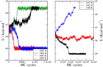
Figure 1: Total energy (in kcal per ion mol) versus MC cycles for the Tosi-Fumi NaCl at T= 1085 K, 1084 K, 1083 K and 1082 K for the 1024 particles system (left-hand side) and T= 1100 K, 1082 K and 1075 K for the 4000 particles system.

After an equilibration interval of about 10⁴ MC cycles (where the energy stays constant), we observed that when the temperature is below melting the energy decreases until it reaches a plateau with a sudden change of slope, corresponding to the situation where the liquid has fully crystallized. When the temperature is above melting, the energy increases until it reaches a plateau and stays constant: at this stage, the solid has completely melted. The results obtained for the 1024 particles system (left-hand side of Fig. 1) show that when T=1083 K the liquid crystallizes, whereas when T $>$ 1084 K the solid melts: therefore, the estimated melting temperature for the 1024 particles system is $T_{m}$=1083(5) K. The results obtained for the 4000 particles system (right-hand side of Fig. 1) show that when T $<$ 1075 K the liquid crystallizes, whereas when T $>$ 1100 K the solid melts. At T=1082K the energy remains approximately constant. From this we conclude that for the 4000 particles system $T_{m}$=1082(13) K. Thus finite size effects on the melting point of NaCl seems to be small once the system has at least 1000 particles.

Hence, when computing $T_{m}$ for the remaining interaction potentials, we chose a large enough system with 2000 particles. In Fig. 2, we present the time evolution of the total energy of the NaCl/SD and NaCl/JC 2000 particles systems, at 1 bar and at different temperatures.

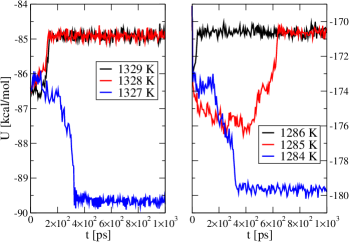
Figure 2: Total energy (in kcal per ion mol) versus time (in picoseconds) for the NaCl/SD system (left-hand side) at T=1329 K, 1328 K and 1327 K, and for the SD/NaCl system (right-hand side) at T= 1284 K, 1285 K and 1286 K. Note the different $y$-axis of both plots.

The results obtained for the 2000 particles system show that the estimated melting temperature is $T_{m}$= 1327(5) K for the NaCl/SD and $T_{m}$=1285(5) K for the NaCl/JC, respectively.

From these results, we can already conclude that the potential that gives the melting temperature closest to the experimental one (1074 K) is the Tosi-Fumi. For this reason the TF/NaCl model is the most suitable for simulations of pure NaCl. This conclusion is further confirmed when calculating the melting curve for both TF/NaCl and JC/NaCl potentials. Using Gibbs Duhem integration Kofke (1993) we calculated the $p-T$ melting curve of the TF/NaCl and the JC/NaCl, presented in Fig. 3.

Figure 3: Melting curve for the TF/NaCl (open diamonds) and JC/NaCl (open circles). Experimental results are from Ref. Boehler et al. (1997) (open squares) and Ref. Akella et al. (1969) (open triangles).

Concerning the results of the TF/NaCl, we observe that at low pressure our calculations recover the experimental slope of the melting curve ($\frac{dp}{dT}=30.6(5)$ bar/K), in good agreement with previous calculations Anwar et al. (2003); Mastny and de Pablo (2005), whereas at higher pressures the slope of the melting line is lower than the experimental one. On the other hand, concerning the results for the JC/NaCl, we observe that not only the melting temperature, but also the slope of the melting curve does not reproduce the experimental one. The same conclusions can be drawn for the melting enthalpy ($\Delta h_{m}$). The calculated melting enthalpies for the TF/NaCl, SD/NaCl and JC/NaCl are 3.36 kcal/mol, 4.8 kcal/mol and 4.6 kcal/mol, respectively, that compared to the experimental value (3.35 kcal/mol), confirms the better performance of the TF/NaCl model with respect to the other models.

IV.2 Route 2. Free-energy calculations

According to the second route, we first computed the Helmholtz free-energy of the solid and liquid phase of the TF/NaCl, and then estimated the Gibbs free-energy of each phase ($G$) by adding the $pV$ term. After that, we performed thermodynamic integration of $G$ in the (p,T) plane at constant pressure as in Eq. 12.

$$\frac{G(T_{2},p)}{Nk_{B}T_{2}}=\frac{G(T_{1},p)}{Nk_{B}T_{1}}-\int_{T_{1}}^{T_{2}}\frac{H(T)}{Nk_{B}T^{2}}dT$$ (12)

where the enthalpy $H(T)=U(T)+pV(T)$ can be easily obtained in NpT simulations at each temperature. The melting point is defined as the state point where the two phases have the same chemical potentials ($\mu=G/N$).

We computed the free-energy of the NaCl solid phase at 1083 K and 1 bar with Einstein crystal (EC) Frenkel and Ladd (1984) and Einstein molecule (EM) Vega and Noya (2007) algorithms. Our results are summarized in Table 2, where we present free-energies in $Nk_{B}T$ units. To determine the normal melting point any temperature could have been selected, the choice of 1083 K is convenient from a practical point of view since it is expected to be close to the T_m of the model, so that to reduce the contribution of the second term on the right side of the Eq. 12.

	$T$[K]	N	$\rho$ (N/Å3)	$\Lambda_{E}[k_{B}T\AA^{-2}]$	A0[NkBT]	$\Delta$ A1[NkBT]	$\Delta$ A2[NkBT]	A${}^{NaCl}_{sol}$[NkBT]
TF/EC	1083	1000	0.03856	500	7.583	-42.73	-6.33	-41.481(9)
TF/EM	1083	1000	0.03856	500	7.594	-42.73	-6.34	-41.477(9)

Table 2: Free energy from the Einstein Crystal/Einstein Molecule for the TF/NaCl solid phase at 1 bar and different temperatures ($T$) and system size ($N$ being the total number of particles). $\rho$ the number density ($N/V$), $\Lambda_{E}$ the spring constant, $A_{0}$, $\Delta A_{1}$, $\Delta A_{2}$ are the terms in Eq. 3 and the free energy of the solid $A^{NaCl}_{sol}$ is represented in the last column and corresponds to Eq.3.

In Table 2, we observe a perfect agreement between the free-energy computed with the Einstein Crystal and the one compute with the Einstein Molecule at the same pressure, temperature and system size (1000 particles).

Having computed the chemical potential of the solid phase, we calculated the Helmholtz free-energy of the liquid phase using two Lennard-Jones reference systems $LJ1$ and $LJ2$ in order to study the uncertainties associated to the choice of the reference system. Results are summarized in Table 3.

	$\Delta$ A${}_{liq}^{LJ}$[NkBT]	A${}_{liq}^{LJ,id}$[NkBT]	A${}_{liq}^{LJ,res}$[NkBT]	A${}_{liq}^{NaCl}$[NkBT]
TF/LJ1	35.95	-5.19	-0.327	-41.47(2)
TF/LJ2	37.12	-5.19	0.837	-41.48(2)

Table 3: TF/NaCl free energy of the liquid phase (A${}_{liq}^{NaCl}$) as in Eq. 5 at 1 bar and T=1083 K. The results presented in the table refer to a system with $N=1000$ particles and number density of $\rho=0.03016$ Å^-3. $\Delta$A^LJ is the integral in Eq. 5. $\frac{A_{liq}^{LJ,id}}{Nk_{B}T}=ln(\rho/2)-1.00$. A${}_{liq}^{LJ,res}$ is obtained from the EOS of Ref. Kolafa and Nezbeda (1994).

As shown in Table 3, the value of the integral ($\Delta$A${}_{liq}^{LJ}$) depends on the choice of the LJ parameters of the reference LJ system. In Fig. 4 the integrand of Eq. 5 is shown when carrying out the thermodynamic integration from the liquid TF/NaCl to both LJ reference systems $LJ1$ and $LJ2$. It is relevant to stress that, due to the abrupt change of $\langle U^{LJ}-U^{NaCl}\rangle_{N,V,T,\lambda}$ for values of $\lambda$ close to 1, many points were used in the integration between $\lambda=0.95$ and $\lambda=1.00$.

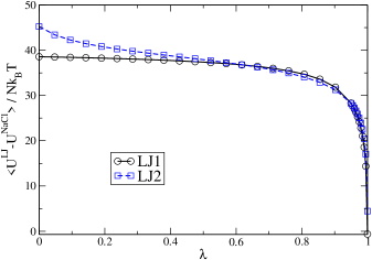
Figure 4: $\langle U^{LJ}-U^{NaCl}\rangle_{N,V,T,\lambda}$ from Eq. 5 at 1083 K and 1 bar. The two curves correspond to a different set of Lennard-Jones parameters for the reference system: $LJ1$ (open circles) and $LJ2$ (open squares).

To calculate the residual free energy of the reference LJ fluid at our thermodynamic conditions, we used the equation of state (EOS) for the LJ system proposed by Nezbeda et al. Kolafa and Nezbeda (1994, 2010). Independently on the chosen reference system (whether $LJ1$ or $LJ2$), the two free-energies A${}_{liq}^{NaCl}$[Nk_BT] coincide (last column in Table 3).

After having computed the Helmholtz free-energy, we estimated the Gibbs free-energy ($G$) by adding the $pV$ term and performed thermodynamic integration of $G$ at constant pressure (see Eq. 12) where we used NpT MC simulations to compute enthalpy $H(T)$ and to estimate the equation of state of the liquid and solid phases (where a typical MC run consists of 3x10⁴ equilibration and 7x10⁴ production cycles). The chemical potential of one phase is $\mu=G/N$ and the melting temperature is given by the point at which the two phases have the same chemical potentials. Our results for the TF/NaCl are presented in Table 4.

	Tm[K]		Tm[K]
TF/LJ1	1083(3)	TF/LJ2	1084(3)

Table 4: Melting temperature at 1 bar of the TF/NaCl model. The results presented in the table refer to a system with $N=1000$ particles. The parameters for the interaction potentials of the reference systems ($LJ1$ and $LJ2$) are given in Table 1.

Both results are in perfect agreement with the T_m calculated by direct coexistence. Other EOS could be used to calculate the residual free energy of the reference LJ fluid, such as the one proposed by Johnson et al. Johnson et al. (1994). When the LJ residual contribution is taken from Johnson et al., the melting temperature turns out to be about 6 K higher than when it is taken from Nezbeda et al. However, it is likely that the EOS proposed by Nezbeda is slightly more accurate than that by Johnson et al. Kolafa and Nezbeda (1994). In any case, the differences are small.

IV.3 Route 3. Hamiltonian Gibbs-Duhem integration

The third route we followed to compute the melting temperature of several alkali halides at 1 bar is by means of the Hamiltonian Gibbs-Duhem thermodynamic integration. We used the TF/NaCl as the reference Hamiltonian ($U_{A}$ in Eq. 7) and integrated the generalized Clapeyron equation (Eq. 11) using a 1000-particle system. From the $\lambda=1$ point of the Hamiltonian Gibbs-Duhem integration, we could compute the melting entropy $\Delta S_{m}$ (being $\Delta S_{m}=N\Delta s_{m}$, see Eq. 10) and the melting enthalpy ($\Delta H_{m}=N\Delta h_{m}$) at coexistence. In the Table 5 we present our results for the melting temperature, $\Delta S_{m}$, reporting also the experimental values of both for each alkali halide, and for $\Delta H_{m}$. We checked our Hamiltonian Gibbs Duhem calculations by computing the melting temperature of TF/KF at 1 bar by means of liquid/solid direct coexistence. Figure 5 represents the time evolution of the total energy of the TF/KF 2000-particle systems, equilibrated at 1 bar and at different temperatures. From these results we estimate T_m to be 860(5) K, that corroborates the result obtained with the Hamiltonian Gibbs Duhem integration in Table 5 (i.e. 859(15)K).

Alkali halide	Tm	T${}^{exp}_{m}$	$\Delta S_{m}$	$\Delta$S${}_{m}^{exp}$	$\Delta H_{m}$	$\Delta$H${}_{m}^{exp}$
NaCl	1082(13)	1074	3.10	3.12	3.36	3.35
KF	859(15)	1131	2.77	2.98	2.39	3.37
KBr	1043(15)	1003	3.14	3.03	3.29	3.04
KCl	1039(15)	1049	3.12	3.04	3.25	3.19
RbBr	1047(15)	955	3.34	2.88	3.51	2.75
RbCl	1092(15)	988	3.18	2.88	3.48	2.85
RbF	996(15)	1048	3.03	2.88	3.03	3.02
NaF	611(15)	1266	2.10	3.09	1.29	3.91
NaBr	1022(15)	1028	3.10	3.06	3.18	3.70
LiCl	780(15)	887	2.46	2.70	1.93	2.39
LiF	1010(15)	1118	2.93	2.88	2.97	3.22

Table 5: Melting temperatures, $\Delta S_{m}$ and $\Delta H_{m}$ at 1 bar for several alkali halides simulated using the TF interaction potential with units T_m($[K]$), $\Delta S_{m}$($[cal/(Kmol)]$) and $\Delta H_{m}$($[kcal/mol]$). The experimental values of $\Delta S_{m}$ are from Ref. Ubbelohde (1978); March and Tosi (1984); Wunderlich (2005). The bold fonts represent alkali halides for which there are good agreement with the experimental melting temperatures.

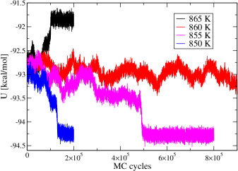
Figure 5: Total energy versus MC cycles for TF/KF at T = 865 K, 860 K, 855 K and 850 K (from top to bottom).

While the Tosi-Fumi potential predicts the NaCl melting temperature in good agreement with its experimental value, the results for the other alkali halides are not as accurate. The predictions for KCl and NaBr are reasonable (differing only about 15 K and 10 K from the experiments). Whereas for alkali halides involving Rb or F ions (such as KF, RbBr, RbCl, RbF, LiF and NaF) the calculated values strongly differ from the experimental ones (with deviations of up to 100 K). From this we conclude that the TF model potential, being non-polarizable, fails when describing alkali halides that involve big cations (such as Rb⁺) and small anions (such as F^-). In general, when T_m of a given TF/alkali halide is lower/higher than the experimental value, also $\Delta H_{m}$ is smaller/larger than the experiments, so that the predicted $\Delta S_{m}$ is in reasonable agreement with the experimental value for most of the studied alkali halides.

V Discussions

We now compare our data for the melting temperature of NaCl at 1 bar with other values taken from the literature (see Table 6).

	Tm[K]	N	$\rho_{liq}$	$\rho_{sol}$
TF/Anwar Anwar et al. (2003)	1064(14)	512	–	–
TF/Anwar* Anwar et al. (2003)	1084(14)	512	–	–
TF/Zykova-Timan Zykova-Timan et al. (2005)	1066(20)	5760	–	–
TF/Mastny Mastny and de Pablo (2005)	1050(3)	512	–	–
TF/Eike Eike et al. (2005)	1089(8)	512	–	–
TF/An An et al. (2006)	1063(13)	4096	–	–
TF/this work	1083(5)	1024	1.465	1.876
TF/this work	1082(13)	4000	1.465	1.876
SD/this work	1327(10)	2000	1.216	1.668
JC/this work	1286(10)	2000	1.283	1.746
Experiments/Janz Janz (1967)	1074	-	1.54	1.98

Table 6: Melting temperature of the NaCl computed using TF, SD and JC interaction potentials at 1 bar. N represents de number of ions of each study. $\rho_{liq}$ and $\rho_{sol}$ are the liquid and solid densities in $gcm^{-3}$, respectively. The * represents the recalculated T_m at 1 bar using the values given by Anwar (p_coex=-300 bar at 1074 K and $\frac{dp}{dT}=30~{}{\rm bar}~{}K^{-1}$).

Concerning the calculations of the melting temperature with the Tosi-Fumi, we observe that $T_{m}$ calculated in this work is in good agreement (within the error bar) with the one reported by Anwar et al. Anwar et al. (2003). They calculated the coexistence pressure at 1074 K and $-300$ bar. Then, they evaluated the slope of the coexistence curve, $\frac{dp}{dT}=30~{}{\rm bar}~{}K^{-1}$, and recalculated the melting temperature at 1 bar obtaining 1064(14) K (nonetheless, using their values, we have obtained the NaCl melting temperature at 1084(14) K, in perfect agreement with our results). Zykova-Timan et al. Zykova-Timan et al. (2005) computed the melting temperature via liquid/solid direct coexistence and obtained a value for T_m in good agreement with the one obtained in this work (taking into account that in their NVE runs they obtained the melting temperature for a pressure of about +- 500 bar and since the slope of the melting curve is of about 30K/bar the value at $p=1bar$ could be modified by up to 17K ). In general, the agreement with data in the literature is satisfactory. The TF slightly underestimates the experimental values of the coexistence densities, whereas both SD and JC underestimate them considerably, in agreement with the results of Alejandre and Hansen for the SD model Alejandre and Hansen (2007).

When computing the melting temperature of the TF/NaCl model potential via liquid/solid direct coexistence and free-energy calculations we have studied finite-size effects and observed that the value of the melting temperature did not change much for systems having more than 1000 particles. Thus we take T_m=1082(13) K (i.e the melting point of the 4000 particle system ) as our estimate of the melting point of the TF/NaCl model potential in the thermodynamic limit ( where the error bar now includes the possible contribution to the error of the extrapolation to infinite size). When calculating T_m via Hamiltonian Gibbs-Duhem integration, we have used the value of T_m=1082(13) K as the initial point for the Hamiltonian Gibbs Duhem integration at coexistence.

Concerning the calculation of the melting temperature with the Smith-Dang and Joung-Cheatham potentials, we computed these values via two independent routes (liquid/solid direct coexistence and Hamiltonian Gibbs-Duhem integration) and obtained the same results. The T_m of both models is reported here. From our calculations we conclude that these models overestimate the melting temperature of NaCl, being about 200-250 K higher than the experimental value of 1074 K. Therefore, it is clear that the melting temperature that most resembles the experimental one at 1 bar is the one calculated using the TF/NaCl. Although JC/NaCl or SD/NaCl would work for NaCl solutions in water, they seem to be unsuitable for simulations of pure NaCl.

VI Conclusions

In this manuscript, we have computed the melting temperature at 1 bar for different NaCl-type alkali halides. When computing T_m for the Tosi Fumi NaCl interaction potential, we have followed three independent routes: 1) liquid/solid direct coexistence, 2) free-energy calculations and 3) Hamiltonian Gibbs-Duhem integration. For the Smith Dang /NaCl and Joung Cheatham NaCl, we have used the first and third route, whereas for other Tosi Fumi alkali halides we have applied only the third route.

The results obtained for the T_m of TF/NaCl are in good agreement with other numerical Anwar et al. (2003); Zykova-Timan et al. (2004) and with experimental results Janz (1967), giving T_m= 1082(13) K at 1 bar. When computing T_m for the SD/NaCl and JC/NaCl, we find a perfect agreement between the calculations obtained via liquid/solid direct coexistence and Hamiltonian Gibbs-Duhem integration. However, both models overestimate the melting temperature of NaCl by more than 200 K. We have also determined the melting curve for the Tosi-Fumi and Joung-Cheatham models and found that the Tosi-Fumi correctly predicts the behavior of the curve ($\frac{dp}{dT}$) at low pressures, but does not capture the experimental behavior when the pressure increases. Therefore, we conclude that the SD/JC models are unable to reproduce the properties of pure NaCl.

We have also computed the melting temperature of other alkali halides using the Tosi-Fumi interaction potential and observed that this model gives good predictions for NaCl, NaBr, KCl and KBr, whereas for the other alkali halides the predictions are not as good, especially when it concerns Rb⁺ and F^- ions. The reason for this probably being that the Tosi-Fumi interaction potential is not polarizable and cannot capture the highly polarizable character of these ions. Neglecting the polarization terms causes an incorrect description of these salts. In the past polarization effects were normally incorporated into the simulations of ionic systems via the shell model Sangster and Dixon (1976). More elaborate models developed recently employ potentials which include the polarization effects using either multipole expansions Wilson and Madden (1992) or the distortable ion model Tangney and Scandolo (2003). The TF/alkali halide potentials have a serious transferability problem: the same ions present different potential parameters depending on the alkali halide (i.e. the Na-Na interaction is different in NaCl and NaF). In the case of LJ-like models, it seems that it is not possible to describe NaCl accurately with a model consisting of point charges and a Lennard-Jones interaction site for each ion where Lorentz-Berthelot rules are used to describe the interaction between cations and anions. The same conclusion was obtained by Cavallari et al. Cavallari et al. (2004) who showed how the ion-ion interaction reconstructed from standard LB rules fail to correctly account for the structure of the concentrated solutions model with ab-initio calculations. An interesting possibility would be incorporating deviations to the Lorentz-Berthelot combining rules to obtain the crossed interactions between the ions or adjusting these interactions as in the TF model, although probably the use of a Van der Waals r^-6 term would not capture the underlying physics. Thus, it seems there is still room for improvement in the area of alkali-halides salt models.

VII acknowledgments

This work was funded by grants FIS2010-16159. from the DGI (Spain), MODELICO-P2009/ESP/1691 from the CAM, and 910570 from the UCM. J. L. Aragones would like to thank the MEC by the award of a pre-doctoral grant. C.Valeriani acknowledgments financial support from a Juan de la Cierva Fellowship and from a PCIG-GA-2011-303941 Marie Curie Integration Grant. E. Sanz acknowledgments financial support from a Ramon y Cajal Fellowship. We would like to thank the referees for their helpful comments.

References

- Groth et al. (1998) B. Groth, R. Evans, and S. Dietrich, Phys. Rev. E 57, 6944 (1998).
- Orkoulas and Panagiotopoulos (1999) G. Orkoulas and A. Z. Panagiotopoulos, J. Chem. Phys. 110 (1999).
- Ciach and Stell (2004) A. Ciach and G. Stell, Phys. Rev. E 70, 016114 (2004).
- Hynninen et al. (2006) A. P. Hynninen, M. E. Leunissen, A. van Blaaderen, and M. Dijkstra, Phys. Rev. Lett. 96, 018303 (2006).
- Gonzalez-Melchor et al. (2003) M. Gonzalez-Melchor, J. Alejandre, and F. Bresme, Phys. Rev. Lett. 90, 135506 (2003).
- Vega et al. (1996) C. Vega, F. Bresme, and J. L. F. Abascal, Phys. Rev. E 54, 2746 (1996).
- Vega et al. (2003) C. Vega, J. L. F. Abascal, C. McBride, and F. Bresme, J. Chem. Phys. 119, 964 (2003).
- Born and Verh (1919) M. Born and D. Verh, Verhandl. Deut. Physik. Ges. 21, 13 (1919).
- Pauling (1928a) L. Pauling, Zeitschrift für Kristallographie 67, 377 (1928a).
- Pauling (1928b) L. Pauling, J. Am. Chem. Soc. 50, 1036 (1928b).
- Mayer (1933) J. E. Mayer, J. Chem. Phys. 1, 270 (1933).
- Huggins and Mayer (1933) M. L. Huggins and J. E. Mayer, J. Chem. Phys. 1, 643 (1933).
- Fumi and Tosi (1964) F. Fumi and M. Tosi, Journal of Physics and Chemistry of Solids 25, 31 (1964).
- Lewis et al. (1975) J. Lewis, K. Singer, and L. Woodcock, J. Chem. Soc. Faraday Trans. 71, 301 (1975).
- Wilson and Madden (1992) M. Wilson and P. Madden, J. Phys. Cond. Mat. 5, 2687 (1992).
- Adams and McDonald (1974) D. Adams and I. McDonald, J. Phys. C: Solid State Phys. 7, 2761 (1974).
- Valeriani et al. (2005) C. Valeriani, E. Sanz, and D. Frenkel, J. Chem. Phys. 122, 194501 (2005).
- Chen et al. (2004) K. Chen, X. Zhu, and J. Wang, Chinese journal of Inorganic Chemistry 20, 1050 (2004).
- Zhu (2004) X. Zhu, J. Molec. Structure-Theochem. 680, 137 (2004).
- Zykova-Timan et al. (2004) T. Zykova-Timan, U. Tartaglino, D. Ceresoli, W. Sekkal-Zaoui, and E. Tosatti, Surf. Sci. 566-568, 794 (2004).
- T.Zykova-Timan et al. (2008) T.Zykova-Timan, C.Valeriani, E.Sanz, D.Frenkel, and E.Tosatti, Phys. Rev. Lett. 100, 036103 (2008).
- Anwar et al. (2003) J. Anwar, D. Frenkel, and M. G. Noro, J. Chem. Phys. 118, 728 (2003).
- Eike et al. (2005) D. M. Eike, J. F. Brennecke, and E. J. Maginn, J. Chem. Phys. 122, 014115 (2005).
- Mastny and de Pablo (2005) E. Mastny and J. de Pablo, J. Chem. Phys. 122, 124109 (2005).
- Zykova-Timan et al. (2005) T. Zykova-Timan, D.Ceresoli, U. Tartaglino, and E. Tosatti, J. Chem. Phys. 125, 164701 (2005).
- Boehler et al. (1997) R. Boehler, M. Ross, and D. Boercker, Phys. Rev. Lett. 78, 4589 (1997).
- Boehler et al. (1996) R. Boehler, M. Ross, and D. Boercker, Phys. Rev. B 53, 556 (1996).
- Belonoshko et al. (2000) A. Belonoshko, R. Ahuja, and B. Johansson, Phys. Rev. B 61, 11928 (2000).
- Belonoshko and Dubrovinsky (1996) A. Belonoshko and L. Dubrovinsky, Am. Mineral. 81, 303 (1996).
- Smith and Dang (1994) D. E. Smith and L. X. Dang, J. Chem. Phys. 100, 3757 (1994).
- Dang and Smith (1993) L. Dang and D. E. Smith, J. Chem. Phys. 99, 6950 (1993).
- Joung and Cheatham (2008) I. Joung and T. Cheatham, J. Phys. Chem. B 112, 9020 (2008).
- Vrbka and Jungwirth (2007) L. Vrbka and P. Jungwirth, J. Molec. Liq. 134, 64 (2007).
- Corradini et al. (2010) D. Corradini, M. Rovere, and P. Gallo, J. Chem. Phys. 132, 134508 (2010).
- Corradini et al. (2011) D. Corradini, M. Rovere, and P. Gallo, J. Phys. Chem. B 115, 1461 (2011).
- Poole et al. (1992) P. H. Poole, F. Sciortino, U. Essmann, and H. E. Stanley, Nature 360, 324 (1992).
- Moucka et al. (2011) F. Moucka, M. Lisal, J. Skvor, J. Jirsak, I. Nezbeda, and W. Smith, J. Phys. Chem. B 115, 7849 (2011).
- Sanz and Vega (2007) E. Sanz and C. Vega, J. Chem. Phys. 126, 014507 (2007).
- Aragones et al. (2012) J. L. Aragones, E. Sanz, and C. Vega, J. Chem. Phys. 136, 244508 (2012).
- Joung and Cheatham (2009) I. Joung and T. Cheatham, J. Phys. Chem. B 113, 13279 (2009).
- Lisal et al. (2005) M. Lisal, W. Smith, and J. Kolafa, J. Phys. Chem. B 109, 12956 (2005).
- Paluch et al. (2010) A. S. Paluch, S. Jayaraman, J. K. Shah, and E. J. Maginn, J. Chem. Phys. 133, 124505 (2010).
- Moucka et al. (2012) F. Moucka, M. Lisal, and W. R. Smith, J. Phys. Chem. B 116, 5468 (2012).
- Adams and McDonald (1975) D. Adams and I. McDonald, Physica B 79, 159 (1975).
- (45) See EPAPS Document No. E-JCPS for a complete description of the parameters of the Tosi-Fumi potential for alkali halides, and for the parameters of the Smith-Dang and Joung-Cheatam models of NaCl. (????).
- Lorentz (1881) H. A. Lorentz, Annalen der Physik 12 pp, 127 (1881).
- Berthelot (1898) D. Berthelot, Comptes rendus 126, 1703 (1898).
- Ladd and Woodcock (1977) A. J. C. Ladd and L. V. Woodcock, Chem. Phys. Lett. 51, 155 (1977).
- Ladd and Woodcock (1978) A. J. C. Ladd and L. V. Woodcock, Molec. Phys. 36, 611 (1978).
- Morris and Song (2002) J. R. Morris and X. Song, J. Chem. Phys. 116, 9352 (2002).
- Yoo et al. (2004) S. Yoo, X. C. Zeng, and J. R. Morris, J. Chem. Phys. 120, 1654 (2004).
- Karim and Haymet (1988) O. A. Karim and A. D. J. Haymet, J. Chem. Phys. 89, 6889 (1988).
- Noya et al. (2008a) E. G. Noya, C. Vega, and E. de Miguel, J. Chem. Phys. 128, 154507 (2008a).
- Fernandez et al. (2006) R. G. Fernandez, J. L. F. Abascal, and C. Vega, J. Chem. Phys. 124, 144506 (2006).
- Rozmanov and Kusalik (2011) D. Rozmanov and P. G. Kusalik, Phys. Chem. Chem. Phys. 13, 15501 (2011).
- Weiss et al. (2011) V. C. Weiss, M. Rullich, C. Kohler, and T. Frauenheim, J. Chem. Phys. 135, 034701 (2011).
- Frenkel and Ladd (1984) D. Frenkel and A. J. C. Ladd, J. Chem. Phys. 81, 3188 (1984).
- Vega and Noya (2007) C. Vega and E. G. Noya, J. Chem. Phys. 127, 154113 (2007).
- Noya et al. (2008b) E. G. Noya, M. M. Conde, and C. Vega, J. Chem. Phys. 129, 104704 (2008b).
- Vega et al. (2008) C. Vega, E. Sanz, E. G. Noya, and J. L. F. Abascal, J. Phys. Condens. Matter 20, 153101 (2008).
- Kolafa and Nezbeda (1994) J. Kolafa and I. Nezbeda, Fluid Phase Equilibria 100, 1 (1994).
- Johnson et al. (1993) J. K. Johnson, J. A. Zollweg, and K. E. Gubbins, Molec. Phys. 78, 591 (1993).
- Agrawal and Kofke (1995a) R. Agrawal and D. A. Kofke, Phys. Rev. Lett. 74, 122 (1995a).
- Agrawal and Kofke (1995b) R. Agrawal and D. A. Kofke, Molec. Phys. 85, 23 (1995b).
- Vega et al. (2005) C. Vega, E. Sanz, and J. L. F. Abascal, J. Chem. Phys. 122, 114507 (2005).
- Frenkel and Smit (2002) D. Frenkel and B. Smit, Understanding Molecular Simulation (Academic Press, London, 2002).
- Allen and Tildesley (1987) M. P. Allen and D. J. Tildesley, Computer Simulation of Liquids (Oxford University Press, 1987).
- der Spoel et al. (2005) D. V. der Spoel, E. Lindahl, B. Hess, G. Groenhof, A. E. Mark, and H. J. C. Berendsen, J. Comput. Chem. 26, 1701 (2005).
- Nosé (1984) S. Nosé, Molec. Phys. 52, 255 (1984).
- Hoover (1985) W. G. Hoover, Phys. Rev. A 31, 1695 (1985).
- Parrinello and Rahman (1981) M. Parrinello and A. Rahman, J. Appl. Phys. 52, 7182 (1981).
- Kofke (1993) D. A. Kofke, J. Chem. Phys. 98, 4149 (1993).
- Akella et al. (1969) J. Akella, S. Vaidya, and G. Kennedy, Phys. Rev. 185, 1135 (1969).
- Kolafa and Nezbeda (2010) J. Kolafa and I. Nezbeda, Sklogwiki www.sklogwiki.org (2010).
- Johnson et al. (1994) J. K. Johnson, E. A. Muller, and K. E. Gubbins, J. Phys. Chem. 98, 6413 (1994).
- Ubbelohde (1978) A. Ubbelohde, in The molten state of matter melting and crystal structure (John Wiley and Sons, 1978).
- March and Tosi (1984) N. March and M. Tosi, in Coulomb liquids (Academic Press, 1984).
- Wunderlich (2005) B. Wunderlich, in Thermal analysis of polymeric materials (Springer, 2005).
- An et al. (2006) Q. An, L. Zheng, R. Fu, S. Ni, and S.Luo, J. Chem. Phys. 125, 154510 (2006).
- Janz (1967) G. Janz, in Molten Salts Handbook (Academic Press, 1967).
- Alejandre and Hansen (2007) J. Alejandre and J. Hansen, Phys. Rev. E 76, 061505 (2007).
- Sangster and Dixon (1976) M. Sangster and M. Dixon, Adv. Phys. 23, 247 (1976).
- Tangney and Scandolo (2003) P. Tangney and S. Scandolo, J. Chem. Phys. 119, 9673 (2003).
- Cavallari et al. (2004) M. Cavallari, C. Cavazzoni, and M. Ferrario, Molec. Phys. 102, 959 (2004).