Active Learning for Crowd-Sourced Databases

Abstract

Crowd-sourcing has become a popular means of acquiring labeled data for many tasks where humans are more accurate than computers, such as image tagging, entity resolution, or sentiment analysis. However, due to the time and cost of human labor, solutions that solely rely on crowd-sourcing are often limited to small datasets (i.e., a few thousand items). This paper proposes algorithms for integrating machine learning into crowd-sourced databases in order to combine the accuracy of human labeling with the speed and cost-effectiveness of machine learning classifiers. By using active learning as our optimization strategy for labeling tasks in crowd-sourced databases, we can minimize the number of questions asked to the crowd, allowing crowd-sourced applications to scale (i.e, label much larger datasets at lower costs).

Designing active learning algorithms for a crowd-sourced database poses many practical challenges: such algorithms need to be generic, scalable, and easy-to-use for a broad range of practitioners, even those who are not machine learning experts. We draw on the theory of nonparametric bootstrap to design, to the best of our knowledge, the first active learning algorithms that meet all these requirements.

Our results, on $3$ real-world datasets collected with Amazon’s Mechanical Turk, and on $15$ UCI datasets, show that our methods on average ask $1$–$2$ orders of magnitude fewer questions than the baseline, and $4.5$–$44\times$ fewer than existing active learning algorithms.

1 Introduction

Crowd-sourcing marketplaces, such as Amazon’s Mechanical Turk, have made it easy to recruit a crowd of people to perform tasks that are difficult for computers, such as entity resolution [5, 7, 35, 42, 53], image annotation [51], and sentiment analysis [37]. Many of these tasks can be modeled as database problems, where each item is represented as a row with some missing attributes (labels) that the crowd workers supply. This has given rise to a new generation of database systems, called crowd-sourced databases [23, 26, 35, 39], that enable users to issue more powerful queries by combining human-intensive tasks with traditional query processing techniques. Figure 1 provides a few examples of such queries, where part of the query is processed by the machine (e.g., whether the word “iPad” appears in a tweet) while the human-intensive part is sent to the crowd for labeling (e.g., to decide if the tweet has a positive sentiment).

While query optimization techniques [23, 34, 38, 39] can reduce the number of items that need to be labeled, any crowd-sourced database that solely relies on human-provided labels will eventually suffer from scalability issues when faced with web-scale datasets and problems (e.g., daily tweets or images). This is because labeling each item by humans can cost several cents and take several minutes. For instance, given the example of Figure 1, even if we filter out tweets that do not contain “iPad”, there could still be millions of tweets with “iPad” that require sentiment labels (‘positive’ or ‘non-positive’).

To enable crowd-sourced databases to scale up to large datasets, we advocate combining humans and machine learning algorithms (e.g., classifiers), where (i) the crowd labels items that are either inherently difficult for the algorithm, or if labeled, will form the best training data for the algorithm, and (ii) the (trained) algorithm is used to label the remaining items much more quickly and cheaply. In this paper, we focus on labeling algorithms (classifiers) that assign one of several discrete values to each item, as opposed to predicting numeric values (i.e., regression), or finding missing items [48], leaving these other settings for future work.

Specifically, given a large, unlabeled dataset (say, millions of images) and a classifier that can attach a label to each unlabeled item (after sufficient training), our goal is to determine which questions to ask the crowd in order to (1) achieve the best training data and overall accuracy, given time or budget constraints, or (2) minimize the number of questions, given a desired level of accuracy.

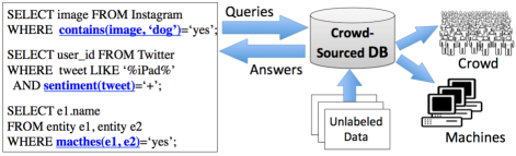
Figure 1: Examples of Labeling Queries in a Crowd-sourced DB.

Our problem is closely related to the classical problem of active learning (AL), where the objective is to select statistically optimal training data [15]. However, in order for an AL algorithm to be a practical optimization strategy for labeling tasks in a crowd-sourced database, it must satisfy a number of systems challenges and criteria that have not been a focal concern in traditional AL literature, as described next.

1.1 Design Criteria

An AL algorithm must meet the following criteria to be used as the default optimization strategy in a crowd-sourced database:

• 1. Generality. Our system must come with a few built-in AL algorithms that are applicable to arbitrary classification and labeling tasks, as crowd-sourced systems are used in a wide range of different domains. In Figure 1, for example, one query involves sentiment analysis while another seeks images containing a dog. Clearly, these tasks require drastically different classifiers. Although our system allows expert users to provide their own custom-designed AL that works for their classification algorithm, most users may only have a classifier. Thus, to support general queries, our AL algorithm should make minimal or no assumptions about the classifiers that users provide with their labeling tasks.

• 2. Black-box treatment of the classifier. Many AL algorithms that provide theoretical guarantees, need to access and modify the internal logic of the given classifier (e.g., adding constraints to the classifier’s internal loss-minimization step [8]). Such modifications are acceptable in theoretical settings but not in real-world applications, as state-of-the-art classifiers used in science and industry are rarely a straightforward implementation of textbook algorithms. Rather, these finely-tuned classifiers typically use thousands of lines of code to implement many intertwined steps (e.g., data cleaning, feature selection, parameter tuning, heuristics, etc.). In some cases, moreover, these codebases use proprietary libraries that cannot be modified. Thus, to make our crowd-sourcing system useful to a wide range of practitioners and scientists (who are not necessarily machine learning experts), we need an AL algorithm that treats the classifier as a black-box, i.e., no modifications to the internals of the classifier.

• 3. Batching. Many (theoretical) AL algorithms are designed for online (a.k.a. streaming) scenarios in which items are revealed one at a time. This means that the AL algorithm decides whether to request a label for the current item, and if so, awaits the label before proceeding to the next item. While these settings are attractive for theoretical reasons, they are unrealistic in practice. First, we often have access to a large pool of unlabeled data to choose from (not just the next item), which should allow us to make better choices. Second, online AL settings typically perform an (expensive) analysis for each item [8, 9, 16], rendering them computationally prohibitive. Thus, for efficiency and practicality, the AL algorithm must support batching, so that (i) the analysis is done only once per each batch of multiple items, and (ii) items are sent to the crowd in batches (to be labeled in parallel).

• 4. Parallelism. We aim to achieve human-scalability (i.e., asking the crowd fewer questions) through AL. However, we are also concerned with machine-scalability, because AL often involves repeatedly training a classifier and can thus be computationally expensive. While AL has been historically applied to small datasets, increasingly massive datasets (such as those motivating this paper) pose new computational challenges. Thus, a design criterion in our system is that our AL algorithm must be amenable to parallel execution on modern many-core processors and distributed clusters.

• 5. Noise management. AL has traditionally dealt with expert-provided labels that are often taken as ground truth (notable exceptions are agnostic AL approaches [16]). In contrast, crowd-provided labels are subject to a greater degree of noise, e.g., innocent errors, typos, lack of domain knowledge, and even deliberate spamming.

AL has a rich literature in machine learning [43]. However, the focus has been largely theoretical, with concepts from learning theory used to establish bounds on sample complexity, but leaving a significant gap between theory and practice. Rather than aiming at such theoretical bounds, this paper focuses on a set of practical design criteria and provides sound heuristics for the AL problem; the origin of these criteria is in real-world and systems considerations (in particular, issues of scale and ease-of-use).

To the best of our knowledge, no existing AL algorithm satisfies all of the aforementioned requirements. For example, those AL algorithms that are general [8, 9, 16] do not support batching or parallelism and often require modifications to the classifier. (See Section 7 for a detailed literature review.) In this paper, we design the first AL algorithms that meet all these design criteria, paving the way towards a scalable and generic crowd-sourcing system that can be used by a wide range of practitioners.

1.2 Our Contributions

Our main contributions are two AL algorithms, called MinExpError and Uncertainty, along with a noise-management technique, called partitioning-based allocation (PBA). The Uncertainty algorithm requests labels for the items that the classifier is most uncertain about. We also design a more sophisticated algorithm, called MinExpError, that combines the current quality (say, accuracy) of the classifier with its uncertainty in a mathematically sound way, in order to choose the best questions to ask. Uncertainty is faster than MinExpError, but it also has lower overall accuracy, especially in the upfront scenario, i.e., where we request all labels in a single batch. We also study the iterative scenario, i.e., where we request labels in multiple batches and refine our decisions after receiving each batch.

A major novelty of our AL algorithms is in their use of bootstrap theory, which yields several key advantages. First, bootstrap can deliver consistent estimates for a large class of estimators, making our AL algorithms general and applicable to nearly any classification task. Second, bootstrap-based estimates can be obtained while treating the classifier as a complete black-box. Finally, the required bootstrap computations can be performed independently from each other, hence, allowing for an embarrassingly parallel execution.

Once MinExpError or Uncertainty decides which items to send to the crowd, dealing with the inherent noise in crowd-provided labels is the next challenge. A common practice is to use redundancy, i.e., to ask each question to multiple workers. However, instead of applying the same degree of redundancy to all items, we have developed a novel technique based on integer linear programming, called PBA, which dynamically partitions the unlabeled items based on their degree of difficulty for the crowd and determines the required degree of redundancy for each partition.

Thus, with a careful use of bootstrap theory as well as our batching and noise-management techniques, our AL algorithms meet all our requirements for building a practical crowd-sourced system, namely generality, scalability (batching and parallelism), and ease-of-use (black-box view and automatic noise-management).

We have evaluated the effectiveness of our algorithms on $18$ real-world datasets ($3$ crowd-sourced using Amazon Mechanical Turk, and $15$ well-known datasets from the UCI KDD repository). Experiments show that our AL algorithms achieve the same quality as several existing approaches while significantly reducing the number of questions asked of the crowd. Specifically, on average, we reduce the number of questions asked by:

• $100\times$ ($7\times$) in the upfront (iterative) scenario, compared to passive learning, and

• $44\times$ ($4.5\times$) in the upfront (iterative) scenario, compared to IWAL [2, 8, 9] which is the state-of-the-art general-purpose AL algorithm.

Interestingly, we also find that our algorithms (which are general-purpose) are still competitive with, and sometimes even superior to, some of the state-of-the-art domain-specific (i.e., less general) AL techniques. For example, our algorithms ask:

• $7\times$ fewer questions than CrowdER [53] and an order of magnitude fewer than CVHull [7], which are among the most recent AL algorithms for entity resolution in database literature,

• $2$–$8\times$ fewer questions than Bootstrap-LV [41] and MarginDistance [49], and

• $5$–$7\times$ fewer questions for SVM classifiers than AL techniques that are specifically designed for SVM [49].

2 Overview of Approach

Our approach in this paper is as follows. The user provides (i) a pool of unlabeled items (possibly with some labeled items as initial training data), (ii) a classifier (or “learner”) that improves with more and better training data, and a specification as to whether learning should be upfront or iterative, and (iii) a budget or goal, in terms of time, quality, or cost (and a pricing scheme for paying the crowd).

Our system can operate in two different scenarios, upfront or iterative, to train the classifier and label the items (Section 2.2). Our proposed AL algorithms, Uncertainty and MinExpError, can be used in either scenario (Section 3). Acquiring labels from a crowd raises interesting issues, such as how best to employ redundancy to minimize error, and how many questions to asked the crowd (Sections 4 and 5). Finally, we empirically evaluate our algorithms (Section 6).

2.1 Active Learning Notation

An active learning algorithm is typically composed of (i) a ranker $\mathcal{R}$, (ii) a selection strategy $\mathcal{S}$, and (iii) a budget allocation strategy $\Gamma$. The ranker $\mathcal{R}$ takes as input a classification algorithm $\theta$, a set of labeled items $L$, and a set of unlabeled items $U$, and returns as output an “effectiveness” score $w_{i}$ for each unlabeled item $u_{i}\in U$. Our proposed algorithms in Section 3 are essentially ranking algorithms that produce these scores. A selection strategy then uses the scores returned from the ranker to choose a subset $U^{\prime}\subseteq U$ which will be sent for human labeling. For instance, one selection strategy is picking the top $k$ items with the largest (or smallest) scores, where $k$ is determined by the budget or quality requirements. In this paper, we use weighted sampling to choose $k$ unlabeled items, where the probability of choosing each item is proportional to its score. Finally, once $U^{\prime}$ is chosen, a budget allocation strategy $\Gamma$ decides how to best acquire labels for all the items in $U^{\prime}$: $\Gamma(U^{\prime},B)$ for finding the most accurate labels given a fixed budget $B$, or $\Gamma(U^{\prime},Q)$ for the cheapest labels given a minimum quality requirement $Q$. For instance, to reduce the crowd noise, a common strategy is to ask each question to multiple labelers and take the majority vote. In Section 4, we introduce our Partitioning Based Allocation (PBA) algorithm, which will be our choice of $\Gamma$ in this paper.

2.2 Active Learning Scenarios

This section describes how learning works in the upfront and the iterative scenarios. Suppose we have a given budget $B$ for asking questions (e.g., in terms of money, time, or number of questions) or a quality requirement $Q$ (e.g., required accuracy or F1-measure) that our classifier must achieve.

The choice of the scenario depends on user’s preference and needs. Figure 2 is the pseudocode of the upfront scenario. In this scenario, the ranker computes effectiveness scores solely based on the initial labeled data, $L_{0}$. Then, a subset $U^{\prime}\subseteq U$ is chosen and sent to the crowd (based on $\mathcal{S}$ and, $B$ or $Q$). While waiting for the crowd to label $U^{\prime}$ (based on $\Gamma$ and, $B$ or $Q$), we train our classifier $\theta$ on $L_{0}$ to label the remaining items, namely $U-U^{\prime}$, and immediately send their labels back to the user. Once crowd-provided labels arrive, they are also sent to the user. Thus, the final result consists of the union of these two labeled sets.

Figure 3 shows the pseudocode of the iterative scenario. In this scenario, we ask for labels in several iterations. We ask the crowd to label a few items, adding those labels to the existing training set, and retrain. Then, we choose a new set of unlabeled items and iterate until we have exhausted our budget $B$ or met our quality goal $Q$. At each iteration, our allocation strategy ($\Gamma$) seeks the cheapest or most accurate labels for the chosen items ($U^{\prime}$), then our ranker uses the original training data $L_{0}$ as well as the crowd labels $CL$ collected thus far to decide how to score the remaining unlabeled items.

Note that the upfront scenario is not an iterative scenario with a single iteration, because the former does not use the crowd-sourced labels in training the classifier. This difference is important as different applications may call for different scenarios. When early answers are strictly preferred, say in an interactive search interface, the upfront scenario can immediately feed users with model-provided labels until the crowd’s answers arrive for the remaining items. The upfront scenario is also preferred when the project has a stringent accuracy requirement that only gold data (here, $L_{0}$) be used for training the classifier, say to avoid the potential noise of crowd labels in the training phase. In contrast, the iterative scenario is computationally slower, as it has to repeatedly retrain a classifier and wait for crowd-sourced labels. However, it can adaptively adjust its scores in each iteration, thus achieving a smaller error for the same budget than the upfront one. This is because the upfront scenario must choose all the items it wants labeled at once, based only on a limited set of initial labels.

Upfront Active Learning ($B$ or $Q$, $L_{0},U,\theta,\mathcal{R},\mathcal{S},\Gamma$)
Input: $B$ is the total budget (money, time, or number of questions),
		$Q$ is the quality requirement (e.g., minimum accuracy, F1-measure),
		$L_{0}$ is the initial labeled data,
		$U$ is the unlabeled data,
		$\theta$ is a classification algorithm to (imperfectly) label the data,
		$\mathcal{R}$ is a ranker that gives “effectiveness” scores to unlabeled items,
		$\mathcal{S}$ is a selection strategy (specifying which items should be labeled
		by the crowd, given their effectiveness scores).
		$\Gamma$ is a budget allocation strategy for acquiring labels from the crowd
Output: $L$ is the labeled version of $U$
1:	$W\leftarrow\mathcal{R}(\theta,L_{0},U)$    //$w_{i}\in W$ is the effectiveness score for $u_{i}\in U$
2:	Choose $U^{\prime}\subseteq U$ based on $\mathcal{S}(U,W)$ such that $U^{\prime}$ can be labeled with
3:			budget $B$  or  $\theta^{L_{0}}(U-U^{\prime})$ satisfies $Q$
4:	$M$$L$$\leftarrow\theta^{L_{0}}(U-U^{\prime})$    //train $\theta$ on $L_{0}$ to automatically label $U-U^{\prime}$
5:	Immediately display $ML$ to the user    //Early query results
6:	$CL\leftarrow\Gamma(U^{\prime},B$ or $Q)$    //Ask (and wait for) the crowd to label $U^{\prime}$
7:	$L\leftarrow CL\cup ML$    //combine crowd and machine provided labels
Return $L$

Figure 2: The upfront scenario in active learning.

Iterative Active Learning ($B$ or $Q$, $L_{0},U,\theta,\mathcal{R},\mathcal{S},\Gamma$)
Input: Same as those in Figure 2)
Output: $L$ is the labeled version of $U$
1:	$CL\leftarrow\emptyset$    // labeled data acquired from the crowd
2:	$L\leftarrow\theta^{L_{0}}(U)$    //train $\theta$ on $L_{0}$ & invoke it to label $U$
3:	While our budget $B$ is not exhausted or $L$’s quality does not meet $Q$:
4:		$W\leftarrow\mathcal{R}(\theta,L_{0}\cup CL,U)$    //$w_{i}\in W$ is the effective score for $u_{i}\in U$
5:		Choose $U^{\prime}\subseteq U$ based on $\mathcal{S}(U,W)$   (subject to $B$ or $Q$)
6:		$L^{\prime}\leftarrow\Gamma(U^{\prime},B$ or $Q)$    //Ask (and wait for) the crowd to label $U^{\prime}$
7:		$CL\leftarrow CL\cup L^{\prime}$,   $U\leftarrow U-U^{\prime}$ //remove crowd labels from $U$
8:		$L\leftarrow CL\cup\theta^{L_{0}\cup CL}(U)$   //train $\theta$ on $L_{0}\cup CL$ to label remaining $U$
Return $L$

Figure 3: The iterative scenario in active learning.

3 Ranking Algorithms

This paper proposes two novel AL algorithms, Uncertainty and MinExpError. AL algorithms consist of (i) a ranker $\mathcal{R}$ that assigns scores to unlabeled items, (ii) a selection strategy $\mathcal{S}$ that uses these scores to choose which items to label, and (iii) a budget allocation strategy $\Gamma$ to decide how to acquire crowd labels for those chosen items. As explained in Section 2.1, our AL algorithms use weighted sampling and PBA (introduced in Section 4) as their selection and budget allocation strategies, respectively. Thus, for simplicity, we use Uncertainty and MinExpError to refer to both our AL algorithms and their corresponding rankers. Both rankers can be used in either upfront or iterative scenarios. Section 3.1 provides brief background on nonparametric bootstrap theory, which we use in our rankers. Our rankers are introduced in Sections 3.2 and 3.3.

3.1 Background: Nonparametric Bootstrap

Our ranking algorithms rely on nonparametric bootstrap (or simply the bootstrap) to assess the benefit of acquiring labels for different unlabeled items. Bootstrap [20] is a powerful statistical technique traditionally designed for estimating the uncertainty of estimators. Consider an estimator $\theta$ (say, a classifier) that can be learned from data $L$ (say, some training data) to estimate some value of interest for a data point $u$ (say, the class label of $u$). This estimated value, denoted as $\theta^{L}(u)$, is a point-estimate (i.e., a single value), and hence, reveals little information about how this value would change if we used a different data $L^{\prime}$. This information is critical as most real-world datasets are noisy, subject-to-change, or incomplete. For example, in our active learning context, missing data means that we can only access part of our training data. Thus, $L$ should be treated a random variable drawn from some (unknown) underlying distribution $\mathbb{D}$. Consequently, statisticians are often interested in measuring distributional information about $\theta^{L}(u)$, such as variance, bias, etc. Ideally, one could measure such statistics by (i) drawing many new datasets, say $L_{1},\cdots,L_{k}$ for some large $k$, from the same distribution $\mathbb{D}$ that generated the original $L$, (ii) computing $\theta^{L_{1}}(u),\cdots,\theta^{L_{k}}(u)$, and finally (iii) inducing a distribution for $\theta(u)$ based on the observed values of $\theta^{L_{i}}(u)$. We call this true distribution $D^{\theta}(u)$ or simply $D(u)$ when $\theta$ is understood. Figure 4(a) illustrates this computation. For example, when $\theta$ is a binary classifier, $D(u)$ is simply a histogram with two bins ($0$ and $1$), where the value of the $i$’th bin for $i\in\{0,1\}$ is $Pr[\theta^{L}(u)=i]$ when $L$ is drawn from $\mathbb{D}$. Given $D(u)$, any distributional information (e.g., variance) can be obtained.

Unfortunately, in practice the underlying distribution $\mathbb{D}$ is often unknown, and hence, direct computation of $D(u)$ using the procedure of Figure 4(a) is impossible. This is where bootstrap [20] becomes useful. The main idea of bootstrap is simple: treat $L$ as a proxy for its underlying distribution $\mathbb{D}$. In other words, instead of drawing $L_{i}$’s directly from $\mathbb{D}$, generate new datasets $S_{1},\cdots,S_{k}$ by resampling from $L$ itself. Each $S_{i}$ is called a (bootstrap) replicate or simply a bootstrap. Each $S_{i}$ is generated by drawing $n=|L|$ I.I.D. samples with replacement from $L$, and hence, some elements of $L$ might be repeated or missing in $S_{i}$. Note that all bootstraps have the same cardinality as $L$, i.e. $|S_{i}|=|L|$ for all $i$. By computing $\theta$ on these bootstraps, namely $\theta^{S_{1}}(u),\cdots,\theta^{S_{k}}(u)$, we can create an empirical distribution $\hat{D}(u)$. This is the bootstrap computation, which is visualized in Figure 4(b).

The theory of bootstrap guarantees that for a large class of estimators $\theta$ and sufficiently large $k$, we can use $\hat{D}(u)$ as a consistent approximation of $D(u)$. The intuition is that, by resampling from $L$, we emulate the original distribution $\mathbb{D}$ that generated $L$. Here, it is sufficient (but not necessary) that $\theta$ be relatively smooth (i.e., Hadamard differentiable [20]) which holds for a large class of machine learning algorithms [30] such as $M$-estimators, themselves including maximum likelihood estimators and most classification techniques. In our experiments (Section 6), $k$=$100$ or even $10$ have yielded reasonable accuracy ($k$ can also be tuned automatically; see [20]).

Both of our AL algorithms use bootstrap to estimate the classifier’s uncertainty in its predictions (say, to stop asking the crowd once we are confident enough). Employing bootstrap has several key advantages. First, as noted, bootstrap delivers consistent estimates for a large class of estimators, making our AL algorithms general and applicable to nearly any classification algorithm. Second, the bootstrap computation uses a “plug-in” principle; that is, we simply need to invoke our estimator $\theta$ with $S_{i}$ instead of $L$. Thus, we can treat $\theta$ (here, our classifier) as a complete black-box since its internal implementation does not need to be modified. Finally, individual bootstrap computations $\theta^{S_{1}}(u),\cdots,\theta^{S_{k}}(u)$ are independent from each other, and hence can be executed in parallel. This embarrassingly parallel execution model enables scalability by taking full advantage of modern many-core and distributed systems.

Thus, by exploiting powerful theoretical results from classical nonparametric statistics, we can estimate the uncertainty of complex estimators and also scale up the computation to large volumes of data. Aside from Provost et al. [41] (which is limited to probabilistic classifiers and is less effective than our algorithms; see Sections 6 and 7), no one has exploited the power of bootstrap in AL, perhaps due to bootstrap’s computational overhead. However, with recent advances in parallelizing and optimizing bootstrap computation [3, 27, 55, 56] and increases in RAM sizes and the number of CPU cores, bootstrap is now a computationally viable approach, motivating our use of it in this paper.

3.2 Uncertainty Algorithm

Our Uncertainty algorithm aims to ask the crowd the questions that are hardest for the classifier. Specifically, we (i) find out how uncertain (or certain) our given classifier $\theta$ is in its label predictions for different unlabeled items, and (ii) ask the crowd to label items for which the classifier is least certain. The intuition is that, the more uncertain the classifier, the more likely it will mislabel the item.

Note that focusing on most uncertain items is one of the oldest ideas in AL literature [15, 47]. The novelty and power of our Uncertainty algorithm is in its use of bootstrap for obtaining an unbiased estimate of uncertainty, while making almost no assumptions about the classification algorithm. Previous proposals that capture uncertainty either (i) require a probabilistic classifier that can produce highly accurate class probability estimates along with its label predictions [41, 51], or (ii) are limited to a particular classifier. For example, the standard way of performing uncertainty-based sampling is by using the entropy of the class distribution in the case of probabilistic classifiers [40, 57]. Although entropy-based AL can be effective in some situations [21, 40, 57], in many other situations, when the classifiers do not produce accurate probabilities, entropy does not guarantee an unbiased estimate of the uncertainty (see Section 6.3). For non-probabilistic classifiers, other heuristics such as the distance from the separator is taken as a measure of uncertainty (e.g., SVM classifiers [49, 52]). However, these heuristics cannot be applied to arbitrary classifiers. In contrast, our Uncertainty algorithm applies to both probabilistic and non-probabilistic classifiers, and is also guaranteed by bootstrap theory to produce unbiased estimates. (In Section 6, we also empirically show that our algorithm is more effective.) Next, we describe how Uncertainty uses bootstrap to estimate the classifier’s uncertainty.

Let $l$ be the predicted label for item $u$ when we train $\theta$ on our labeled data $L$, i.e., $\theta^{L}(u)=l$. As explained in Section 3.1, $L$ is often a random variable, and hence, $\theta^{L}(u)$ has a distribution (and variance). We use the variance of $\theta$ in its prediction, namely $Var[\theta^{L}(u)]$, as our formal notion of uncertainty. Our intuition behind this choice is as follows. A well-established result from Kohavi and Wolpert [28] has shown that the classification error for item $u$, say $e_{u}$, can be decomposed into a sum of three terms:

$$e_{u}=\mbox{Var}[\theta^{L}(u)]+bias^{2}[\theta^{L}(u)]+\sigma^{2}(u)$$

where $bias[.]$ is the bias of the classifier and $\sigma^{2}(u)$ is a noise term. Our ultimate goal in AL is to reduce the sum of $e_{u}$ for all $u$. The $\sigma^{2}(u)$ is an error inherent to the data collection process, and thus cannot be eliminated through AL. Thus, by requesting labels for $u$’s that have a large variance, we indirectly reduce $e_{u}$ for $u$’s that have a large classification error. Hence, our Uncertainty algorithm assigns $\mbox{Var}[\theta^{L}(u)]$ as the score for each unlabeled item $u$, to ensure that items with larger variance are sent to the crowd for labels. Thus, in Uncertainty algorithm, our goal is to measure $\mbox{Var}[\theta^{L}(u)]$.

Since the underlying distribution of the training data ($\mathbb{D}$ in Figure 5) is unknown to us, we use bootstrap. In other words, we bootstrap our current set of labeled data $L$, say $k$ times, to obtain $k$ different classifiers that are then invoked to generate labels for each item $u$. This is shown in Figure 4(b). The output of these classifiers form an empirical distribution $\hat{D}(u)$ that approximates the true distribution of $\theta^{L}(u)$. We can then estimate $\mbox{Var}[\theta^{L}(u)]$ using $\hat{D}(u)$ which is guaranteed, by bootstrap theory [20], to quickly converge to the true value of $\mbox{Var}[\theta^{L}(u)]$ as we increase $k$.

Let $S_{i}$ denote the $i$’th bootstrap, and $\theta^{S_{i}}(u)=l^{i}_{u}$ be the prediction of our classifier for $u$ when trained on this bootstrap. Define $X(u):=\sum_{i=1}^{k}l^{i}_{u}/k$, i.e., the fraction of classifiers in Figure 4(b) that predict a label of $1$ for $u$. Since $l^{i}_{u}\in\{0,1\}$, the uncertainty score for instance $u$ is given by its variance, which can be computed as:

$$Uncertainty(u)=\mbox{Var}[\theta^{L}(u)]=X(u)(1-X(u))$$ (1)

We evaluate our Uncertainty algorithm in Section 6.

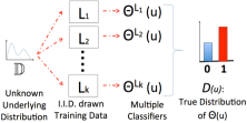
(a) Ideal computation of $D(u)$

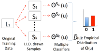
(b) Bootstrap computation

Figure 4: Bootstrap approximation $\hat{D}(u)$ of true distribution $D(u)$.

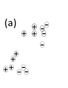
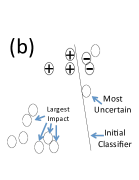
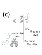
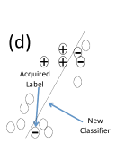
Figure 5: (a) Fully labeled dataset, (b) initial labels, (c) asking hardest
questions, and (d) asking questions with high impact.

3.3 MinExpError Algorithm

Consider the toy dataset of Figure 5. Initially, only a few labels ($+$ or $-$) are revealed to us, as shown in Figure 5. With these initial labels we train a classifier, say a linear separator (shown as a solid line). The Uncertainty algorithm would ask the crowd to label the items with the most uncertainty, here being those closer to the separator. The intuition behind Uncertainty is that, by measuring the uncertainty (and requesting labels for the most uncertain items), the crowd essentially handles items that are hardest (or ambiguous) for the classifier. However, this might not always be the best strategy. By acquiring a label for the item closest to the separator and training a new classifier, as shown in Figure 5, our overall accuracy does not change much: despite acquiring a new label, the new classifier still misclassifies three of the items at the lower-left corner of Figure 5. This observation shows that labeling items with most uncertainty (i.e., asking the hardest questions) may not have the largest impact on the classifier’s prediction power for other data points. In other words, another great strategy would be to acquire human labels for items that, if their labels differ from what the current classifier thinks, would have a huge impact on the classifier’s future decisions. In Figure 5, the lower-left points exemplify such items. We say that such items have a potential for largest impact on the classifier’s accuracy.

Note that we cannot completely ignore uncertainty and choose items only based on their potential impact on the classifier. When the classifier is highly confident of its predicted label, no matter how much impact an opposite label could have on the classifier, acquiring a label for that item wastes resources because the crowd label will most likely agree with that of the classifier anyway. Thus, our MinExpError algorithm combines these two strategies in a mathematically sound way, described next.

Let $l=\theta^{L}(u)$ be the current classifier’s predicted label for $u$. If we magically knew that $l$ was the correct label, we could simply add $\langle u,l\rangle$ to $L$ and retrain the classifier. Let $e_{\textrm{right}}$ be this new classifier’s error. On the other hand, if we somehow knew that $l$ was the incorrect label, we would instead add $\langle u,1-l\rangle$ to $L$ and retrain the classifier accordingly. Let $e_{\textrm{wrong}}$ denote the error of this new classifier. The problem is that (i) we do not know what the true label is, and (ii) we do not know the classifier’s error in either case.

Solving (ii) is relatively easy: in each case we assume those labels and use cross validation on $L$ to estimate both errors, say $\hat{e}_{\textrm{right}}$ and $\hat{e}_{\textrm{wrong}}$. To solve problem (i), we can again use bootstrap to estimate the probability of our prediction $l$ being correct (or incorrect), say $p(u):=Pr[l=l_{u}|u]$, where $l_{u}$ is $u$’s true label. Since we do not know $l_{u}$ (or its distribution), we bootstrap $L$ to train $k$ different classifiers (following Figure 5’s notation). Let $l_{1},\cdots,l_{k}$ be the labels predicted by these classifiers for $u$. Then, $p(u)$ can be approximated as

$$\hat{p}(u)=\frac{\sum_{i=1}^{k}1(l_{i}=l)}{k}$$ (2)

Here, $1(c)$ is the decision function which evaluates to $1$ when condition $c$ holds and to zero otherwise. Intuitively, equation (2) says that the probability of the classifier’s prediction being correct can be estimated by the fraction of classifiers that agree on that prediction, if those classifiers are each trained on a bootstrap of the training set $L$.

Our MinExpError algorithm aims to compute the classifier’s expected error if we use the classifier itself to label each item, and ask the crowd to label those items for which this expected error is larger. This way, the overall expected error will be minimized. To compute the classifier’s expected error, we can average over different label choices:

$$MinExpError(u) = \hat{p}(u)\hat{e}_{\textrm{right}}+(1-\hat{p}(u))\hat{e}_{\textrm{wrong}}$$ (3)

We can break down equation (3) as:

$$MinExpError(u) = \hat{e}_{\textrm{wrong}}-\hat{p}(u)(\hat{e}_{\textrm{wrong}}-\hat{e}_{\textrm{right}})$$ (4)

Assume that $\hat{e}_{\textrm{wrong}}-\hat{e}_{\textrm{right}}\geq 0$ (an analogous decomposition is possible when it is negative). Eq. (4) tells us that if the question is too hard (small $\hat{p}(u)$), we may still ask for a crowd label to avoid a high risk of misclassification on $u$. On the other hand, we may ask a question for which our model is fairly confident (large $\hat{p}(u)$), but having its true label can still make a big difference in classifying other items ($\hat{e}_{\textrm{wrong}}$ is too large). This means that, however unlikely, if our classifier happens to be wrong, we will have a higher overall error if we do not ask for the true label of $u$. Thus, our MinExpError scores naturally combine both the difficulty of the question and how much knowing its answer can improve our classifier.

3.4 Complexity and Scalability

Besides its generality, a major benefit of bootstrap is that each replicate can be shipped to a different node or processor, performing training in parallel. The time complexity of each iteration of Uncertainty is $O(k\cdot T(|U|))$, where $|U|$ is the number of unlabeled items in that iteration, $T(.)$ is the classifier’s training time (e.g., this is cubic in the input size for SVMs), and $k$ is the number of bootstraps. Thus, we only need $k$ nodes to achieve the same run-time as training a single classifier.

MinExpError is more expensive than Uncertainty as it requires a case analysis for each unlabeled item. The time complexity for each iteration of MinExpError is $O((k+|U|)\cdot T(|U|))$. Since unlabeled items can be independently analyzed, the algorithm is still parallelizable. However, MinExpError requires more nodes (i.e., $O(|U|)$ nodes) to achieve the same performance as Uncertainty. As we show in Section 6, this additional overhead is justified in the upfront scenario, given MinExpError’s superior performance at deciding which questions to ask based on a limited set of initially labeled data.

4 Handling Crowd Uncertainty

Crowd-provided labels are subject to a great degree of uncertainty: humans may give incorrect answers due to ambiguity of the question and innocent (or deliberate) errors. This section proposes an algorithm called Partitioning Based Allocation (PBA) that manages and reduces this uncertainty by strategically allocating different degrees of redundancy to different subgroups of the unlabeled items. PBA is our proposed instantiation of $\Gamma$ in the upfront and iterative scenarios (Figures 2 and 3) which given a fixed budget $B$ maximizes the labels’ accuracy, or given a required accuracy, minimizes cost.

Optimizing Redundancy for Subgroups. Most previous AL approaches assume that labels are provided by domain experts and thus perfectly correct (see Section 7). In contrast, incorrect labels are common in a crowd database — an issue conventionally handled by using redundancy, e.g., asking each question to multiple workers and combining their answers for the best overall result. Standard techniques, such as asking for multiple answers and using majority vote or the techniques of Dawid and Skene (DS) [17] can improve answer quality when the crowd is mostly correct, but will not help much if users do not converge to the right answer or converge too slowly. In our experience, crowd workers can be quite imprecise for certain classification tasks. For example, we removed the labels from $1000$ tweets with hand-labeled (“gold data”) sentiment (dataset details in Section 6.1.3), and asked Amazon Mechanical Turk workers to label them again, then measured the workers’ agreement. We used different redundancy ratios ($1,3,5$) and different voting schemes (majority and DS) and computed the crowd’s ability to agree with the hand-produced labels. The results are shown in Table 1.

Voting Scheme	Majority Vote	Dawid & Skene
1 worker/label	67%	51%
3 workers/label	70%	69%
5 workers/label	70%	70%

Table 1: The effect of redundancy (using both majority voting and Dawid and Skene voting) on the accuracy of crowd labels.

In this case, increasing redundancy from $3$ to $5$ labels does not significantly increase the crowd’s accuracy. Secondly, we have noticed that crowd accuracy varies for different subgroups of the unlabeled data. For example, in a different experiment, we asked Mechanical Turk workers to label facial expressions in the CMU Facial Expression dataset, and measured agreement with hand-supplied labels. This dataset consists of $585$ head-shots of $20$ users, each in $32$ different combinations of head positions (straight, left, right, and up), sunglasses (with and without), and facial expressions (neutral, happy, sad, and angry). The crowd’s accuracy was significantly worse when the faces were looking up versus other positions:

Facial orientation	Avg. accuracy
straight	0.6335%
left	0.6216%
right	0.6049%
up	0.4805%

Similar patterns appear in several other datasets, where crowd accuracy is considerably lower for certain subgroups. To exploit these two observations, we developed our PBA algorithm which computes the optimal number of questions to ask about each subgroup by estimating the probability $p_{g}$ with which the crowd correctly classifies items of a given subgroup $g$, and then solves an integer linear program (ILP) to choose the optimal number of questions (i.e., degree of redundancy) for labeling each item from that subgroup, given these probabilities.

Before introducing our algorithm, we make the following observation. To combine answers using majority voting and an odd number of votes, say $2v+1$, for an unlabeled item $u$ with a true label $l$, the probability of the crowd’s combined answer $l^{*}$ being correct is the probability that at most $v$ or fewer workers get the answer wrong. Denoting this probability with $P_{g,(2v+1)}$, we have:

$$\vspace*{-0.1in}P_{g,(2v+1)}=Pr(l=l^{*}|2v+1\text{ votes})=$$

$$\sum_{i=0}^{v}\binom{2v+1}{i}\cdot p_{g}^{2v+1-i}\cdot(1-p_{g})^{i}$$ (5)

where $p_{g}$ is the probability that a crowd worker will correctly label an item in group $g$.

Next, we describe our PBA algorithm, which partitions the items into subgroups and optimally allocates the budget to different subgroups by computing the optimal number of votes per item, $V_{g}$, for each subgroup $g$. PBA consists of three steps:

Step 1. Partition the dataset into $G$ subgroups. This can be done either by partitioning on some low-cardinality field that is already present in the dataset to be labeled (for example, in an image recognition dataset, we might partition by photographer ID or the time of day when the picture was shot), or by using an unsupervised clustering algorithm such as $k$-means. For instance, in the CMU facial expression dataset, we partitioned the images based on user IDs, leading to $G=20$ subgroups, each with roughly $32$ images.

Step 2. Randomly pick $n_{0}$$>$$1$ different data items from each subgroup, and obtain $v_{0}$ labels for each one of them. Estimate $p_{g}$ for each subgroup $g$, either by choosing data items for which the label is known and computing the fraction of labels that are correct, or by taking the majority vote for each of the $n_{0}$ items, assuming it is correct, and then computing the fraction of labels that agree with the majority vote. For example, for the CMU dataset, we asked for $v_{0}=9$ labels for $n_{0}=2$ random images from each subgroup, and hand-labeled those $n_{0}$$*$$G=40$ images to estimate $p_{g}$ for $g=1,\dots,20$.

Step 3. Solve an ILP to find the optimal $V_{g}$ for every group $g$. We use $b_{g}$ to denote the budget allocated to subgroup $g$, and create a binary indicator variable $x_{gb}$ whose value is 1 iff subgroup $g$ is allocated a budget of $b$. Also, let $f_{g}$ be the number of items that our leaner has chosen to label from subgroup $g$. Our ILP formulation depends on the user’s goal:

Goal 1. Suppose we are given a budget $B$ (in terms of the number of questions) and our goal is to acquire the most accurate labels for the items requested by the learner. We can then formulate an ILP to minimize the following objective function:

$$\sum_{g=1}^{G}\sum_{b=1}^{b^{max}}x_{gb}\cdot(1-P_{g,b})\cdot f_{g}$$ (6)

where $b^{max}$ is the maximum number of votes that we are willing to ask per item. This goal function captures the expected weighted error of the crowd, i.e., it has a lower value when we allocate a larger budget ($x_{gb}$=$1$ for a large $b$ when $P_{g}$$>$$0.5$) to subgroups whose questions are harder for the crowd ($P_{g,b}$ is small) or the learner has chosen more items from that group ($f_{g}$ is large). This optimization is subject to the following constraints:

$$\forall 1\leq g\leq G,~{}~{}~{}\sum_{b=1}^{b^{max}}x_{gb}=1$$ (7)

$$\sum_{g=1}^{G}\sum_{b=1}^{b^{max}}x_{gb}\cdot b\cdot f_{g}\leq B-v_{0}\cdot n_{0}\cdot G$$ (8)

Here, constraint (7) ensures that we pick exactly one $b$ value for each subgroup and (8) ensures that we stay within our  labeling budget (we subtract the initial cost of estimating $p_{g}$’s from $B$).

Goal 2. If we are given a minimum required accuracy $Q$, and our goal is to minimize the total number of questions asked, we modify the formulation above by turning (8) into a goal and (6) into a constraint, i.e., minimizing $\sum_{g=1}^{G}\sum_{b=1}^{b^{max}}x_{gb}\cdot b\cdot f_{g}$ while ensuring that $\sum_{g=1}^{G}\sum_{b=1}^{b^{max}}x_{gb}\cdot(1-P_{g,b})\cdot f_{g}\leq 1-Q$.

Note that one could further improve the $p_{g}$ estimates and the expected error estimate in (6) by incorporating the past accuracy of individual workers [6]. Such extensions are omitted here due to lack of space and left to future work. We evaluate PBA in Section 6.2.

Balancing Classes. Our final observation about the crowd’s accuracy is that crowd workers perform better at classification tasks when the number of instances from each class is relatively balanced. For example, given a face labeling task asking the crowd to tag each face as “man” or “woman” where only $0.1\verb=$ of images are of men, crowd workers will have a higher error rate when labeling men (i.e., the rarer class). Perhaps workers become conditioned to answering “woman”. (Psychological studies report the same effect [54].)

Interestingly, both our Uncertainty and MinExpError algorithms naturally tend to increase the fraction of labels they obtain for rare classes. Since our algorithms tend to have more uncertainty about items with rare labels (due to insufficient examples in their training set), they are more likely to ask users to label those items. Thus, our algorithms naturally improve the “balance” in the questions they ask about different classes, which in turn improves crowd labeling performance. We show this effect in Section 6.2 as well.

5 Optimizing for the Crowd

The previous section described our algorithm for handling noisy labels. There are other optimization questions that arise in practice. How should we decide when our accuracy is “good enough”? (Section 5.1) Given that a crowd can label multiple items in parallel, what is the the effect of batch size (number of simultaneous questions) on our learning performance? (Section 5.2)

5.1 When To Stop Asking

As mentioned in Section 2.2, users may either provide a fixed budget $B$ or a minimum quality requirement $Q$ (e.g., F1-measure). Given a fixed budget, we can ask questions until the budget is exhausted. However, to achieve a quality level $Q$, we must estimate the current error of the trained classifier. The easiest way to do this is to measure the trained classifier’s ability to accurately classify the gold data according to the desired quality metric. We can then continue to ask questions until a specific accuracy on the gold data is achieved (or until the rate of improvement of accuracy levels off).

In the absence of (sufficient) gold data, we adopt the standard $k$-fold cross validation technique, randomly partitioning the crowd-labeled data into test and training sets, and measuring the ability of a model learned on training data to predict test values. We repeat this procedure $k$ times and take the average as an overall assessment of the model’s quality. Section 6.2 shows that this method provides more reliable estimates of the model’s current quality than relying on a small amount of gold data.

5.2 Effect of Batch Sizes

At each iteration of the iterative scenario, we must choose a subset of the unlabeled items according to their effectiveness scores, and send them to the crowd for labeling. We call this subset a “batch” (denoted as $U^{\prime}$ in Line 5 of Figure 3). An interesting question is how to set this batch size, say $\beta$.

Intuitively, a smaller $\beta$ increases opportunities to improve the AL algorithm’s effectiveness by incorporating previously requested labels before deciding which labels to request next. For instance, best results are achieved when $\beta$$=$$1$. However, larger batch sizes reduce the overall run-time substantially by (i) allowing several workers to label items in parallel, and (ii) reducing the number of iterations. This is confirmed by our experiments in Section 6.2, which show that the impact of increasing $\beta$ on the effectiveness of our algorithms is not as dramatic as its impact on the overall run-time. Thus, to find the optimal $\beta$, a reasonable choice is to start from a smaller batch size and continuously increase it (say, double it) until the run-time becomes reasonable, or the quality metric falls below the minimum requirement.

6 Experimental Results

This section evaluates the effectiveness of our AL algorithms in practice by comparing the speed, cost, and accuracy with which our AL algorithms can label a dataset compared to state-of-the-art AL algorithms.

Overview of the Results. Overall, our experiments show the following: (i) our AL algorithms require several orders of magnitude fewer questions to achieve the same quality than the random baseline, and substantially fewer questions ($4.5\times$–$44\times$) than the best general-purpose AL algorithm (IWAL [2, 8, 9]), (ii) our MinExpError algorithm works better than Uncertainty in the upfront setting, but the two are comparable in the iterative setting, (iii) Uncertainty has a much lower computational overhead than MinExpError, and (iv) surprisingly, even though our AL algorithms are generic and widely applicable, they still perform comparably to and sometimes much better than AL algorithms designed for specific tasks, e.g., $7\times$ fewer questions than CrowdER [53] and an order of magnitude fewer than CVHull [7] (two of the most recent AL algorithms for entity resolution), competitive results to Brew et al [13], and also $2$–$8\times$ fewer questions than less general AL algorithms (Bootstrap-LV [41] and MarginDistance [49]).

Experimental Setup. All algorithms were tested on a Linux server with dual-quad core Intel Xeon 2.4 GHz processors and 24GB of RAM. Throughout this section, unless stated otherwise, we repeated each experiment $20$ times and reported the average result, every task cost 1¢, and the size of the initial training and the batch size were $0.03\verb=$ and $10\verb=$ of the unlabeled set, respectively.

Methods Compared. We ran experiments on the following learning algorithms in both the upfront and iterative scenarios:

1. Uncertainty: Our method from Section 3.2.

2. MinExpError: Our method from Section 3.3.

3. IWAL: A popular AL algorithm [9] that follows Importance Weighted Active Learning [8], recently extended with batching [2].

4. Bootstrap-LV: Another bootstrap-based AL that uses the model’s class probability estimates to measure uncertainty [41]. This method only works for probabilistic classifiers, e.g., we exclude this in experiments with SVMs.

5. CrowdER: One of the most recent AL techniques specifically designed for entity resolution tasks [53].

6. CVHull: Another state-of-the-art AL specifically designed for entity resolution [7].

7. MarginDistance: An AL algorithm specifically designed for SVM classifiers, which picks items that are closer to the margin [49].

8. Entropy: A common AL strategy [43] that picks items for which the entropy of different class probabilities is higher, i.e., the more uncertain the classifier, the more similar the probabilities of different classes, and the higher the entropy.

9. Brew et al. [13]: a domain-specific AL designed for sentiment analysis, which uses clustering to select an appropriate subset of articles (or tweets) to be tagged by users.

10. Baseline: A passive learner that randomly selects unlabeled items to send to the crowd.

In the plots, we prepend the scenario name to the algorithm names, e.g., UpfrontMinExpError or IterativeBaseline. We have repeated our experiments with different classifiers as the underlying learner, including SVM, Naïve-Bayes classifier, neural networks, and decision trees. For lack of space, we only report each experiment for one type of classifier. When not specified, we used linear SVM.

Evaluation Metrics. AL algorithms are usually evaluated based on their learning curve, which plots the quality measure of interest (e.g., accuracy or F1-measure) as a function of the number of data items that are labeled [43]. To compare different learning curves quantitatively, the following metrics are typically used:

1. Area under curve (AUC) of the learning curve.

2. AUCLOG, which is the AUC of the learning curve when the X-axis is in log-scale.

3. Questions saved, which is the ratio of number of questions asked by an active learner to those asked by the baseline to achieve the same quality.

Higher AUCs indicate that the learner achieves a higher quality for the same cost/number of questions. Due to the diminishing-return of learning curves, the average quality improvement is usually in a $0$–$16\verb=$ range.

AUCLOG favors algorithms that improve the metric of interest early on (e.g., with few examples). Due to the logarithm, the improvement of this measure is typically in the $0$–$6\verb=$ range.

To compute question savings, we average over all the quality levels that are achievable by both AL and baseline curves. For competent active learners, this measure should (greatly) exceed $1$, as a ratio $<1$ indicates a performance worse than that of the random baseline.

6.1 Crowd-sourced Datasets

We experiment with several datasets labeled using Amazon Mechanical Turk. In this section, we report the performance of our algorithms on each of them.

6.1.1 Entity Resolution

Entity resolution (ER) involves finding different records that refer to the same entity, and is an essential step in data integration/cleaning [5, 7, 35, 42, 53]. Humans are typically more accurate at ER than classifiers, but also slower and more expensive [53].

We used the Product (http://dbs.uni-leipzig.de/file/Abt-Buy.zip) dataset, which contains product attributes (name, description, and price) of items listed on the abt.com and buy.com websites. The task is to detect pairs of items that are identical but listed under different descriptions on the two websites (e.g., “iPhone White 16 GB” vs “Apple 16GB White iPhone 4”). We used the same dataset as [53], where the crowd was asked to label $8315$ pairs of items as either identical or non-identical. This dataset consists of $12\verb=$ identical pairs and $88\verb=$ non-identical pairs. In this dataset, each pair has been labeled by $3$ different workers, with an average accuracy of $89\verb=$ and an F1-measure of $56\verb=$. We also used the same classifier used in [53], namely a linear SVM where each pair of items is represented by their Levenshtein and Cosine similarities. When trained on $3\verb=$ of the data, this classifier has an average accuracy of $80\verb=$ and an F1-measure of $40\verb=$. Figure 8 shows the results of using different AL algorithms. As expected, while all methods eventually improve with more questions, their overall F1-measures improve at different rates. MarginDistance, MinExpError, and CrowdER are all comparable, while Uncertainty improves much more quickly than the others. Here, Uncertainty can identify the items about which the model has the most uncertainty and get the crowd to label those earlier on. Interestingly, IWAL, which is a generic state-of-the-art AL, performs extremely poorly in practice. CVHull performs equally poorly, as it internally relies on IWAL as its AL subroutine. This suggests opportunities for extending CVHull to rely on other AL algorithms in future work.

This result is highly encouraging: even though CrowdER and CVHull are recent AL algorithms highly specialized for improving the recall (and indirectly, F1-measure) of ER, our general-purpose AL algorithms are still quite competitive. In fact, Uncertainty uses $6.6\times$ fewer questions than CrowdER and an order of magnitude fewer questions than CVHull to achieve the same F1-measure.

6.1.2 Image Search

Vision-related problems also utilize crowd-sourcing heavily, e.g., in tagging pictures, finding objects, and identifying bounding boxes [51]. In all of our vision experiments, we employed a relatively simple classifier where the PHOW features (a variant of dense SIFT descriptors commonly used in vision tasks [11]) of a set of images are first extracted as a bag of words, and then a linear SVM is used for their classification. Even though this is not the state-of-the-art image detection algorithm, we show that our AL algorithms still greatly reduce the cost of many challenging vision tasks.

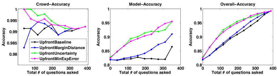
Figure 6: The object detection task (detecting the gender of the person in an image): accuracy of the (a) crowd, (b) model, (c) overall.

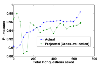
Figure 7: Estimating quality with $k$-fold cross validation.

Gender Detection. We used the faces from Caltech101 dataset [22] and manually labeled each image with its gender (266 males, 169 females) as our ground truth. We also gathered crowd labels by asking the gender of each image from $5$ different workers. We started by training the model on a random set of $11\verb=$ of the data. In Figure 6, we show the accuracy of the crowd, the accuracy of our machine learning model, and the overall accuracy of the model plus crowd data. For instance, when a fraction $x$ of the labels were obtained from the crowd, the other $1-x$ labels were determined from the model, and thus, the overall accuracy was $x*a_{c}+(1-x)*a_{m}$, where $a_{c}$ and $a_{m}$ are the crowd and model’s accuracy, respectively. As in our entity resolution experiments, our algorithms improve the quality of the labels provided by the crowd, i.e., by asking questions for which the crowd tends to be more reliable. Here, though, the crowd produces higher overall quality than in the entity resolution case and therefore its accuracy is improved only from $98.5$% to $100\verb=$. Figure 6 shows that both MinExpError and Uncertainty perform well in the upfront scenario, respectively improving the baseline accuracy by $4\verb=$ and $2\verb=$ on average, and improving its AUCLOG by $2$-$3\verb=$. Here, due to the upfront scenario, MinExpError saves the most number of questions. The baseline has to ask $4.7\times$ ($3.7\times$) more questions than MinExpError (Uncertainty) to achieve the same accuracy. Again MarginDistance, although specifically designed for SVM, achieves little improvement over the baseline.

Object Containment. We again mixed $50$ human faces and $50$ background images from Caltech101 [22]. Because differentiating human faces from background clutter is easy for humans, we used the crowd labels as ground truth in this experiment. Figure 11 shows the upfront scenario with an initial set of $10$ labeled images, where both Uncertainty and MinExpError lift the baseline’s F1-measure by $16\verb=$, while MarginDistance provides a lift of 13%. All three algorithms increase the baseline’s AUCLOG by $5$-$6\verb=$. Note that the baseline’s F1-measure degrades slightly as it reaches higher budgets, since the baseline is forced to give answers to hard-to-classify questions, while the AL algorithms avoid such questions, leaving them to the last batch (which is answered by the crowd).

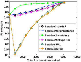
Figure 8: Comparison of different AL algorithms for entity resolution: the overall F1-measure in the iterative scenario.

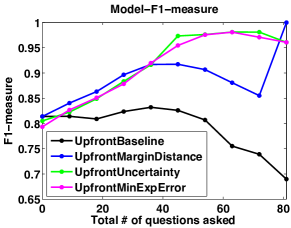
Figure 9: Image search task (whether a scene contains a human): F1-measure of the model.

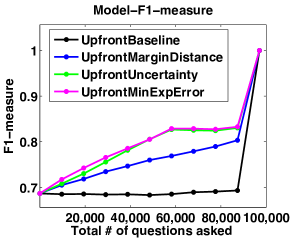
Figure 10: Sentiment analysis task: F1-measure of the model for $100$K tweets.

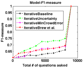
Figure 11: Sentiment analysis task: F1-measure of the model for $10$K tweets.

6.1.3 Sentiment Analysis

Microblogging sites such as Twitter provide rich datasets for sentiment analysis [37], where analysts can ask questions such as “how many of the tweets mentioning iPhone have a positive or negative sentiment?” Training accurate classifiers requires sufficient accurately labeled data, and with millions of daily tweets, it is too costly to ask the crowd to label all of them. In this experiment, we show that our AL algorithms, with as few as $1$K-$3$K crowd-labeled tweets, can achieve very high accuracy and F1-measure on a corpus of $10$K-$100$K unlabeled tweets. We randomly chose these tweets from an online corpus that provides ground truth labels for the tweets, with equal numbers of positive and negative-sentiment tweets. We obtained crowd labels (positive, negative, neutral, or vague/unknown) for each tweet from $3$ different workers.

Figure 11 shows the results for using $1$K initially labeled data points with the $100$K dataset in the upfront setting. The results confirm that the upfront scenario is best handled by our MinExpError Algorithm. Here, the MinExpError, Uncertainty and MarginDistance algorithms improve the average F1-measure of the baseline model by $11\verb=$, $9\verb=$ and $5\verb=$, respectively. Also, MinExpError increases baseline’s AUCLOG by $4\verb=$. All three AL algorithms dramatically reduce the number of questions required to achieve a given accuracy or F1-measure. In comparison to the baseline, MinExpError, Uncertainty, and MarginDistance reduce the number of questions by factors of $46\times$, $32\times$, and $27\times$, respectively.

Figure 11 shows similar results for using $1$K initially labeled tweets with the $10$K dataset but in the iterative setting. The results confirm that the iterative scenario is best handled by our Uncertainty algorithm, which even improves on Brew et al. algorithm [13], which is a domain-specific AL designed for sentiment analysis. Here, the Uncertainty, MinExpError, and Brew et al. algorithms improve the average F1-measure of the baseline model by $9\verb=$, $4\verb=$ and $4\verb=$, respectively. Also, Uncertainty increases baseline’s AUCLOG by $4\verb=$. In comparison to the baseline, Uncertainty, MinExpError, and Brew et al. reduce the number of questions by factors of $5.38\times$, $1.76\times$, and $4.87\times$, respectively. Again, the savings are expectedly modest compared to the upfront scenario.

6.2 PBA and other Crowd Optimizations

In this section, we present results for our crowd-specific optimizations described in Section 5.

PBA Algorithm: We first report experiments on the PBA algorithm. Recall that this algorithm partitions the items into subgroups and optimally allocates the budget amongst them. In the CMU facial expressions dataset, the crowd had a particularly hard time telling the facial expression of certain individuals, so we created subgroups based on the user column of the dataset, and asked the crowd to label the expression on each face. By choosing $v_{0}$=$9$ and $b^{max}$=$9$, we varied $n_{0}=2,4,8,16,32$ and measured the point-wise error of our $P_{g,b}$ estimates. Figure 16 shows that the average error of our estimates drops quickly as the sample size $n_{0}$ increases: the error is $0.22$ for $n_{0}$=$2$ and goes down to $0.13$ with only $n_{0}$=$8$. Also, curve fitting shows that the error is proportional to $O(1/n_{0})$ (like most aggregates).

Choosing $v_{0}=9$, $b^{max}=9$, and $n_{0}=2$, we also compared PBA against a uniform budget allocation scheme, where the same number of questions are asked about all items uniformly, as done in previous research (see 7). The results are shown in Figure 17. Here, the X axis shows the normalized budget, e.g., a value of $2$ means the budget was twice the total number of unlabeled items. The Y axis shows the overall (classification) error of the crowd using majority voting under different allocations. Here, the solid lines show the actual error achieved under both strategies, while the blue and green dotted lines show our estimates of their performance before running the algorithms. From Figure 17, we see that although our estimates of the actual error are not highly accurate, since we only use them to solve an ILP that would favor harder subgroups, our PBA algorithm (solid green) still reduces the overall crowd error by about $10\verb=$ (from $45\verb=$ to $35\verb=$). We also show how PBA would perform if it had an oracle that provided access to exact values of $P_{g,b}$ (red line).

Figure 12: Improving the crowd’s F1-measure for entity resolution in the iterative scenario.

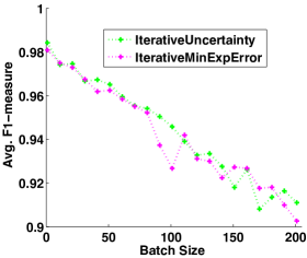
Figure 13: Effect of batch size on our algorithms’ F1-measure (vehicle dataset, w/ a budget of 400 questions).

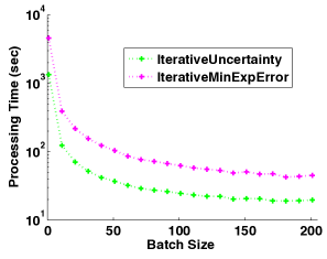
Figure 14: Effect of batch size on our algorithms’ processing times (vehicle dataset, w/ a budget of 400 questions).

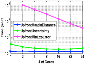
Figure 15: Effect of parallelism on processing time: 100K tweets.

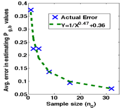
Figure 16: The effect of sample size on the accuracy of $P_{g,b}$ estimates in the PBA algorithm.

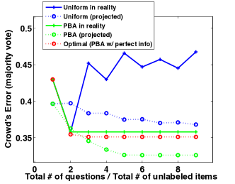
Figure 17: Reducing the crowd’s noise under different budget allocation schemes.

Balancing Classes: Recall from Section 4 that our algorithms tend to ask more questions about rare classes than common classes, which can improve the overall performance. Figure 14 reports the crowd’s F1-measure in an entity resolution task under different AL algorithms. The dataset used in this experiment has many fewer positive instances ($11\verb=$) than negative ones ($89\verb=$). The main observation here is that although the crowd’s average F1-measure for the entire dataset is $56\verb=$ (this is achieved by the baseline), our Uncertainty algorithm can lift this up to $62\verb=$, mainly because the questions posed to the crowd have a balanced mixture of positive and negative labels.

k-Fold Cross Validation for Estimating Accuracy: We use k-fold cross validation to estimate the current quality of our model. Figure 7 shows our estimated F1-measure for an SVM classifier on UCI’s cancer dataset. Our estimates are reasonably close to the true F1 values, especially as more labels are obtained from the crowd. This suggests that k-fold cross validation allows us to effectively estimate current model accuracy, and to stop acquiring more data once model accuracy has reached a reasonable level.

The Effect of Batch Size: We now study the effect of batch size on result quality, based on the observations in Section 5.2. The effect is typically moderate (and often linear), as shown in Figure 14. Here we show that the F1-measure gains can be in the 8–10% range (see Section 5.2). However, larger batch sizes reduce runtime substantially, as Figure 14 shows. Here, going from batch size $1$ to $200$ significantly reduces the time to train a model, by about two orders of magnitude (from $1000$’s of seconds to $10$’s of seconds).

6.3 UCI Classification Datasets

In Section 6.1, we validated our algorithms on crowd-sourced datasets. This section also compares our algorithms on datasets from the UCI KDD [1], where labels are provided by experts; that is, ground truth and crowd labels are the same. Thus, by excluding the effect of noisy labels, we can compare different AL strategies in isolation. We have chosen $15$ well-known datasets, as shown in Figures 18 and 19. To avoid bias, we have avoided any dataset-specific tuning or preprocessing steps, and applied the same classifier with the same settings to all datasets. In each case, we experimented with $10$ different budgets of $10\verb=$ (of total number of labels), each repeated $10$ times, and reported the average. Also, to compute the F1-measure for datasets with more than $2$ classes, we have either grouped all non-majority classes into a single class, or arbitrarily partitioned all the classes into two new ones.

Here, besides the random baseline, we compare Uncertainty and MinExpError against four other AL techniques, namely IWAL,
MarginDistance, Bootstrap-LV, and Entropy. IWAL is as general as our algorithms, MarginDistance only applies to SVM classification, and Bootstrap-LV and Entropy are only applicable to probabilistic classifiers. For all methods (except for MarginDistance) we used MATLAB’s decision trees as the classifier, with its default parameters except for the following: no pruning, no leaf merging, and a ‘minparent’ of $1$ (impure nodes with $1$ or more items can be split).

Figures 18 and 19 show the reduction in the number of questions under both upfront and iterative settings for Entropy, Bootstrap-LV, Uncertainty, and MinExpError, while Table 2 shows the average AUCLOG, F1, and reduction in the number of questions asked across all 15 datasets for all AL methods. The two figures omit detailed results for MarginDistance and IWAL, as they performed poorly (as indicated in Table 2). We report all the measures of different AL algorithms in terms of their performance improvement relative to the baseline (so higher numbers are better). For instance, consider Figure 18. On the yeast dataset, MinExpError reduces the number of questions asked by $84\times$, while Uncertainty and Bootstrap-LV reduce it by about $38\times$ and Entropy does not improve the baseline.

In summary, these results are consistent with those observed with crowd-sourced datasets. In the upfront setting, MinExpError significantly outperforms other AL techniques, with more than $104\times$ savings in the total number of questions on average. MinExpError also improves the AUCLOG and average F1-measure of the baseline on average by $5\verb=$ and $15\verb=$, respectively. After MinExpError, the Uncertainty and Bootstrap-LV are most effective with a comparable performance, i.e. $55$-$69\times$ savings, improving the AUCLOG by $3\verb=$, and lifting the average F1-measure by $11$-$12\verb=$. Bootstrap-LV performs well here, which we expect is due to its use of bootstrap (similar to our algorithms). However, recall that Bootstrap-LV only works for probabilistic classifiers (e.g., decision trees). Here, MarginDistance is only moderately effective, providing around $13\times$ savings. Finally, the least effective algorithms are IWAL and Entropy, which perform quite poorly across almost all datasets. IWAL uses learning theory to establish worst-case bounds on sample complexity (based on VC-dimensions), but these bounds are known to leave a significant gap between theory and practice, as seen here. Entropy relies on the classifier’s own class probability estimates [43], and thus can be quite ineffective when these estimates are highly inaccurate. To confirm this, we used bootstrap to estimate the class probabilities more accurately (similarly to our Uncertainty algorithm), and then computed the entropy of these estimates. The modified version, denoted as Uncertainty (Entropy), is significantly more effective than the baseline ($73\times$), which shows that our idea of using bootstrap in AL not only achieves generality (beyond probabilistic classifiers) but can also improve traditional AL strategies by providing more accurate probability estimates.

For the iterative scenario, Uncertainty actually works better than MinExpError, with an average saving of $7\times$ over the baseline in questions asked and an increase in AUCLOG and average F1-measure by $1\verb=$ and $3\verb=$, respectively. Note that savings are generally more modest than in the upfront case because the baseline receives much more labeled data in the iterative setting and therefore, its average performance is much higher, leaving less room for improvement. However, given the comparable (and even slightly better) performance of Uncertainty compared to MinExpError in the iterative scenario, Uncertainty becomes a preferable choice for this scenario due to its considerably smaller processing overhead (see Section 6.4).

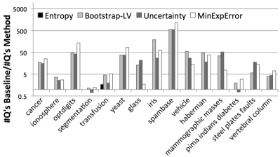
Figure 18: The ratio of the num. of questions asked by the random baseline to those asked by different AL algorithms in the Upfront scenario.

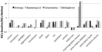
Figure 19: The ratio of the num. of questions asked by the random baseline to those asked by different AL algorithms in the Iterative scenario.

Upfront
Method	AUCLOG(F1)	Avg(Q’s Saved)	Avg(F1)
Uncertainty	1.03x	55.14x	1.11x
MinExpError	1.05x	104.52x	1.15x
IWAL	1.05x	2.34x	1.07x
MarginDistance	1.00x	12.97x	1.05x
Bootstrap-LV	1.03x	69.31x	1.12x
Entropy	1.00x	1.05x	1.00x
Uncertainty (Entropy)	1.03x	72.92x	1.13x
Iterative
Method	AUCLOG(F1)	Avg(Q’s Saved)	Avg(F1)
Uncertainty	1.01x	6.99x	1.03x
MinExpError	1.01x	6.95x	1.03x
IWAL	1.01x	1.53x	1.01x
MarginDistance	1.01x	1.47x	1.00x
Bootstrap-LV	1.01x	4.19x	1.03x
Entropy	1.01x	1.46x	1.01x
Uncertainty (Entropy)	1.01x	1.48x	1.00x

Table 2: Average improvement in AUCLOG, Questions Saved, and Average F1, across all 15 UCI datasets, by different AL algorithms.

6.4 Run-time and Scalability

To measure algorithm runtime, we experimented with multiple datasets. Here, we only report the results for the vehicle dataset. Figure 14 shows that training runtimes range from about $5,000$ seconds to a few seconds and depend heavily on batch size, which determines how many times the model is re-trained.

We also studied the effect of parallelism on our algorithms’ runtimes. Here, we compared different AL algorithms in the upfront scenario on Twitter dataset ($10K$ tweets) as we enabled cores on a multicore machine. The results are shown in Figure 15. Here, for Uncertainty, the run-time only improves until we have as many cores as we have bootstrap replicas (here, 10). After that, improvement is marginal. In contrast, MinExpError scales extremely well, achieving nearly linear speedup because it re-runs the model once for every training point.

Finally, we perform a monetary comparison between our AL algorithms and two different baselines. Figure 20 shows the combined monetary cost (crowd+machines) of achieving different levels of quality (i.e., the Model’s F1-measure for Twitter dataset from Section 6.1.3). The crowd cost is ($0.01$+$0.005$)*$3$ per labeled item, which includes $3\times$ redundancy and Amazon’s commission. The machine cost for the baseline (passive learner) only consists of training a classifier while for our algorithms we have also included the computation of the AL scores. To compute the machine cost, we measured the running time in core-hours using c3.8xlarge instances of Amazon EC2 cloud, which is currently $\$1.68$/hour. The overall cost is clearly dominated by crowd cost, which is why our AL learners can achieve the same quality with a much lower cost (since they ask much fewer questions to the crowd). We also compared against a second baseline where all the items are labeled by the crowd (i.e., no classifiers). As expected, this ‘Crowd Only’ approach is significantly more expensive than our AL algorithms. Figure 21 shows that the crowd can label all the items for $\$363$ with an accuracy of $88.1$–$89.8\verb=$, while we can easily achieve a close accuracy of $\$87.9\verb=$ with only $\$36$ (for labeling $807$ items and spending less than $\$0.00014$ on machine computation). This order of magnitude in saved dollars will only become more dramatic over time, as we expect machine costs to continue dropping according to Moore’s law, while human worker costs will presumably remain the same or even increase.

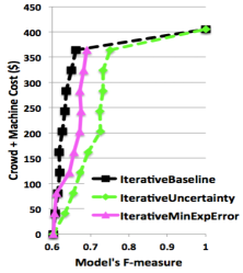
Figure 20: The combined monetary cost of crowd and machines for Twitter dataset.

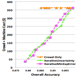
Figure 21: The monetary cost of AL vs. using crowd for all labels.

7 Related Work

Crowd-sourced Databases. These systems [23, 26, 32, 34, 35, 39, 48] use optimization techniques to reduce the number of unnecessary questions asked to humans (e.g., number of pair-wise comparisons in a join or sort query). However, the crowd must still provide at least as many labels as there are unlabeled items directly requested by the user. It is simply unfeasible to label millions of items in this fashion. To scale up to large datasets, we use machine learning to avoid obtaining crowd labels for a significant portion of the data.

Active Learning. AL has been a rich literature in machine learning (see [43]). However, to the best of our knowledge, no existing AL algorithm satisfies all of the desiderata required for a practical crowd-sourced system, namely generality, black-box approach, batching, parallelism, and label-noise management. For example, many AL algorithms are designed for a specific classifier (e.g. neural networks [15] or SVM [49]) or a specific domain (e.g., entity resolution [5, 7, 42, 53], vision [51], or medical imaging [24]). However, our algorithms work for general classification tasks and do not require any domain knowledge. The popular IWAL algorithm [8] is generic (except for hinge-loss classifiers such as SVM), but does not support batching or parallelism, and requires adding new constraints to the classifier’s internal loss-minimization step. In fact, most AL proposals that provide theoretical guarantees (i) are not black-box, as they need to know and shrink the classifier’s hypothesis space at each step, and (ii) do not support batching, as they rely on IID-based analysis. Notable exceptions are [16] and its IWAL variant [9]; they are black-box but they do not support batching or parallelism. Bootstrap-LV [41] and ParaActive [2] support parallelism and batching, but both [2, 9] are based on VC-dimension bounds [10], which are known to be too loose in practice. They cause the model to request many more labels than needed, leading to negligible savings over passive learning (as shown in Section 6). Bootstrap-LV also uses bootstrap, but unlike our algorithms, it is not general. Noisy labelers are handled in [19, 34, 38, 44], but [34, 38, 44] assume the same quality for all labelers and [19] assumes that each labeler’s quality is the same across all items. Moreover, in Section 6, we empirically showed that our algorithms are superior to generic AL algorithms (IWAL +ParaActive [2, 8, 9] and Bootstrap-LV [41]).

AL has been applied to many specific domains (some using crowd-sourcing): machine translation [4], entity resolution [12, 18, 25, 29, 53, 7], and SVM classification [49]. Also, [31] assumes a probabilistic classifier and [13] assumes access to a clustering algorithm for selecting subsets of articles. Our algorithms can handle arbitrary classifiers and do not make any of these assumptions. Also, surprisingly, we are still competitive with (and sometimes even superior to) some of these domain-specific algorithms (e.g., we compared against MarginDistance [49], CrowdER [53], CVHull [7], and Brew et al. [13]).

Semi-supervised Learning. AL and semi-supervised learning (SSL) [33, 46, 50] are closely related. SSL exploits the latent structure of unlabeled data. E.g., [46] combines labeled and unlabeled examples to infer more accurate labels from the crowd. To achieve generality, our PBA algorithm does not assume any prior knowledge of the unlabeled data. Another common SSL technique is to train multiple (ensemble) models with the labeled data to classify the unlabeled data independently, and then use each model’s most confident predictions to train the rest [33, 50]. This is similar to our Uncertainty algorithm, but we use bootstrap, providing a generic way for obtaining multiple predictions and unbiased estimates of uncertainty. Also, we treat the classifier as a black-box, whereas some of these methods do not. However, SSL and AL can be complementary [45], and thus combining them can be an interesting future work to further improve the scalability of crowd-sourced systems.

8 Conclusions

In this paper, we proposed two AL algorithms, Uncertainty and MinExpError, to enable crowd-sourced databases to scale up to large datasets. To broaden their applicability to different classification tasks, we designed these algorithms based on the theory of nonparametric bootstrap and evaluated them in two different settings. In the upfront setting, we ask all questions to the crowd in one go. In the iterative setting, the questions are adaptively picked and added to the labeled pool. Then, we retrain the model and repeat this process. While iterative retraining is more expensive, it also has a higher chance of learning a better model. Additionally, we proposed algorithms for choosing the number of questions to ask different crowd-workers, based on the characteristics of the data being labeled. We also studied the effect of batching on the overall runtime and quality of our AL algorithms. Our results, on three data sets collected with Amazon’s Mechanical Turk, and with $15$ datasets from the UCI KDD archive, show that our algorithms make substantially fewer label requests than state-of-the-art AL techniques. We believe that these algorithms would prove to be immensely useful in crowd-sourced database systems.

References

- [1] D. N. A. Asuncion. UCI machine learning repository, 2007.
- [2] A. Agarwal, L. Bottou, M. Dudík, and J. Langford. Para-active learning. CoRR, abs/1310.8243, 2013.
- [3] S. Agarwal, H. Milner, A. Kleiner, A. Talwalkar, M. Jordan, S. Madden, B. Mozafari, and I. Stoica. Knowing when you’re wrong: Building fast and reliable approximate query processing systems. In SIGMOD Conference, 2014.
- [4] V. Ambati, S. Vogel, and J. Carbonell. Active learning and crowd-sourcing for machine translation. In LREC, volume 1, 2010.
- [5] A. Arasu, M. Götz, and R. Kaushik. On active learning of record matching packages. In SIGMOD, 2010.
- [6] Y. Bachrach, T. Graepel, G. Kasneci, M. Kosinski, and J. Van Gael. Crowd iq: aggregating opinions to boost performance. In AAMS, 2012.
- [7] K. Bellare, S. Iyengar, A. G. Parameswaran, and V. Rastogi. Active sampling for entity matching. In KDD, 2012.
- [8] A. Beygelzimer, S. Dasgupta, and J. Langford. Importance weighted active learning. In ICML, 2009.
- [9] A. Beygelzimer, D. Hsu, J. Langford, and T. Zhang. Agnostic active learning without constraints. In NIPS, 2010.
- [10] C. M. Bishop. Pattern Recognition and Machine Learning. Springer-Verlag New York, Inc., 2006.
- [11] A. Bosch, A. Zisserman, and X. Mu oz. Image classification using random forests and ferns. In ICCV, 2007.
- [12] K. Braunschweig, M. Thiele, J. Eberius, and W. Lehner. Enhancing named entity extraction by effectively incorporating the crowd. In BTW Workshops, 2013.
- [13] A. Brew, D. Greene, and P. Cunningham. Using crowdsourcing and active learning to track sentiment in online media. In ECAI, 2010.
- [14] A. Chatterjee and S. N. Lahiri. Bootstrapping lasso estimators. Journal of the American Statistical Association, 106(494):608–625, 2011.
- [15] D. A. Cohn, Z. Ghahramani, and M. I. Jordan. Active learning with statistical models. J. Artif. Int. Res., 4, 1996.
- [16] S. Dasgupta, D. Hsu, and C. Monteleoni. A general agnostic active learning algorithm. In ISAIM, 2008.
- [17] A. Dawid and A. Skene. Maximum likelihood estimation of observer error-rates using the em algorithm. Applied Statistics, 1979.
- [18] G. Demartini, D. Difallah, and P. Cudré-Mauroux. Large-scale linked data integration using probabilistic crowdsourcing. VLDBJ, 22, 2013.
- [19] P. Donmez, J. G. Carbonell, and J. Schneider. Efficiently learning the accuracy of labeling sources for selective sampling. In KDD, 2009.
- [20] B. Efron and R. J. Tibshirani. An Introduction to the Bootstrap. Chapman & Hall, 1993.
- [21] J. Fan, M. Lu, B. C. Ooi, W.-C. Tan, and M. Zhang. A hybrid machine-crowdsourcing system for matching web tables. In ICDE, 2014.
- [22] L. Fei-Fei, R. Fergus, and P. Perona. Learning generative visual models from few training examples. In WGMBV, 2004.
- [23] M. J. Franklin, D. Kossmann, T. Kraska, S. Ramesh, and R. Xin. Crowddb: answering queries with crowdsourcing. In SIGMOD, 2011.
- [24] S. Hoi, R. Jin, J. Zhu, and M. Lyu. Batch mode active learning and its application to medical image classification. In ICML, 2006.
- [25] L. Jiang, Y. Wang, J. Hoffart, and G. Weikum. Crowdsourced entity markup. In CrowdSem, 2013.
- [26] A. Kittur, B. Smus, S. Khamkar, and R. E. Kraut. Crowdforge: crowdsourcing complex work. In UIST, 2011.
- [27] A. Kleiner and et al. The big data bootstrap. In ICML, 2012.
- [28] R. Kohavi and D. H. Wolpert. Bias plus variance decomposition for zero-one loss functions. In ICML, 1996.
- [29] H. Kopcke, A. Thor, and E. Rahm. Learning-based approaches for matching web data entities. Internet Computing, 14(4), 2010.
- [30] S. Lahiri. On bootstrapping -estimators. Sankhyā. Series A. Methods and Techniques, 54(2), 1992.
- [31] F. Laws, C. Scheible, and H. Schütze. Active learning with amazon mechanical turk. In EMNLP, 2011.
- [32] X. Liu, M. Lu, B. C. Ooi, Y. Shen, S. Wu, and M. Zhang. Cdas: a crowdsourcing data analytics system. PVLDB, 2012.
- [33] P. K. Mallapragada, R. Jin, A. K. Jain, and Y. Liu. Semiboost: Boosting for semi-supervised learning. PAMI, 31, 2009.
- [34] A. Marcus, D. R. Karger, S. Madden, R. Miller, and S. Oh. Counting with the crowd. PVLDB, 2012.
- [35] A. Marcus, E. Wu, D. Karger, S. Madden, and R. Miller. Human-powered sorts and joins. PVLDB, 5, 2011.
- [36] B. Mozafari, P. Sarkar, M. J. Franklin, M. I. Jordan, and S. Madden. Scaling up crowd-sourcing to very large datasets: A case for active learning. PVLDB, 8(2):125–136, 2014.
- [37] A. Pak and P. Paroubek. Twitter as a corpus for sentiment analysis and opinion mining. In Proceedings of LREC, 2010.
- [38] A. G. Parameswaran, H. Garcia-Molina, H. Park, N. Polyzotis, A. Ramesh, and J. Widom. Crowdscreen: algorithms for filtering data with humans. In SIGMOD, 2012.
- [39] H. Park and et al. Deco: A system for declarative crowdsourcing. PVLDB, 5, 2012.
- [40] V. C. Raykar and S. Yu. An entropic score to rank annotators for crowdsourced labeling tasks. In NCVPRIPG, 2011.
- [41] M. Saar-Tsechansky and F. Provost. Active sampling for class probability estimation and ranking. Mach. Learn., 54, 2004.
- [42] S. Sarawagi and A. Bhamidipaty. Interactive deduplication using active learning. In SIGKDD, 2002.
- [43] B. Settles. Active learning literature survey. Computer Sciences Technical Report 1648, University of Wisconsin–Madison, 2010.
- [44] V. Sheng, F. Provost, and P. Ipeirotis. Get another label? In KDD, 2008.
- [45] M. Song, H. Yu, and W.-S. Han. Combining active learning and semi-supervised learning techniques to extract protein interaction sentences. BMC bioinformatics, 12(Suppl 12), 2011.
- [46] W. Tang and M. Lease. Semi-supervised consensus labeling for crowdsourcing. In CIR, 2011.
- [47] S. Tong and D. Koller. Support vector machine active learning with applications to text classification. J. Mach. Learn. Res., 2, 2002.
- [48] B. Trushkowsky, T. Kraska, M. J. Franklin, and P. Sarkar. Crowdsourced enumeration queries. In ICDE, 2013.
- [49] M.-H. Tsai, C.-H. Ho, and C.-J. Lin. Active learning strategies using svms. In IJCNN, 2010.
- [50] H. Valizadegan, R. Jin, and A. K. Jain. Semi-supervised boosting for multi-class classification. In ECML, 2008.
- [51] S. Vijayanarasimhan and K. Grauman. Cost-sensitive active visual category learning. Int. J. Comput. Vision, 91, 2011.
- [52] A. Vlachos. A stopping criterion for active learning. Comput. Speech Lang., 22(3), 2008.
- [53] J. Wang, T. Kraska, M. J. Franklin, and J. Feng. CrowdER: Crowdsourcing entity resolution. PVLDB, 5, 2012.
- [54] J. Wolfe and et al. Low target prevalence is a stubborn source of errors in visual search tasks. Experimental Psychology, 136(4), 2007.
- [55] K. Zeng, S. Gao, J. Gu, B. Mozafari, and C. Zaniolo. Abs: a system for scalable approximate queries with accuracy guarantees. In SIGMOD Conference, 2014.
- [56] K. Zeng, S. Gao, B. Mozafari, and C. Zaniolo. The analytical bootstrap: a new method for fast error estimation in approximate query processing. In SIGMOD Conference, 2014.
- [57] D. Zhou, S. Basu, Y. Mao, and J. C. Platt. Learning from the wisdom of crowds by minimax entropy. In Advances in Neural Information Processing Systems, 2012.