Gas fraction and star formation efficiency at z $<$ 1.0

After new observations of 39 galaxies at z $\sim$ 0.6-1.0 obtained at the IRAM 30m telescope, we present our full CO line survey covering the redshift range 0.2 $<$ z $<$ 1. Our aim is to determine the driving factors accounting for the steep decline in the star formation rate during this epoch. We study both the gas fraction, defined as M_gas/(M_gas+M_star), and the star formation efficiency (SFE) defined by the ratio between far-infrared luminosity and molecular gas mass (L_FIR/M(H₂)), i.e. a measure for the inverse of the gas depletion time. The sources are selected to be ultra-luminous infrared galaxies (ULIRGs), with L_FIR greater than 10¹² L_⊙  and experiencing starbursts. When we adopt a standard ULIRG CO-to-H₂ conversion factor, their molecular gas depletion time is less than 100 Myr. Our full survey has now filled the gap of CO observations in the 0.2$<$z$<$1 range covering almost half of cosmic history. The detection rate in the 0.6 $<$ z $<$ 1 interval is 38% (15 galaxies out of 39), compared to 60% for the 0.2$<$z$<$0.6 interval. The average CO luminosity is L’_CO = 1.8$\times$10¹⁰ K  km s^-1  pc², corresponding to an average H₂  mass of 1.45$\times$10¹⁰ M_⊙. From observation of 7 galaxies in both CO(2-1) and CO(4-3), a high gas excitation has been derived; together with the dust mass estimation, this supports the choice of our low ULIRG conversion factor between CO luminosity and H₂  for our sample sources. We find that both the gas fraction and the SFE significantly increase with redshift, by factors of $3\pm 1$ from z=0 to 1, and therefore both quantities play an important role and complement each other in cosmic star formation evolution.

1 Introduction

The star formation history (SFH) of the Universe shows a steep decline by a factor 10 between z=1 and 0, after a peak of activity around z=1-1.5, well within the first half of the Universe’s age (Madau et al 1998, Hopkins & Beacom 2006). During the second half of the Universe, fundamental changes occur not only in the star formation rate, but also in both the galaxy interaction/merger rate (Le Fèvre et al. 2000, Conselice et al. 2009, Kartaltepe et al. 2010) and the galaxy morphology (Sheth et al. 2008, Conselice et al. 2011), as the well known local Hubble sequence is just now assembling.

The main physical processes causing the decline in the SFH are not well understood. One frequently invoked factor is the gas content, or gas fraction at a given stellar mass, since gas is the fuel for star formation. Locally, the gas fraction for giant spirals is about 7-10% (Leroy et al. 2008, Saintonge et al. 2011a), while at z$\sim$1.2 it increases to 34$\pm$5% and at z$\sim$2.3 to 44$\pm 6$% (Tacconi et al. 2010, Daddi et al. 2010). However, the average surface and volume gas densities should be more relevant factors, and there is evidence of a wide range in gas properties of galaxies at each redshift: molecular gas extents, mean gas densities and star formation efficiencies (Daddi et al. 2008). The average molecular gas density can be traced by the CO excitation, measured from line ratios of the CO ladder (e.g. Weiss et al. 2007). Another intervening factor is an external dynamical trigger of star formation, such as galaxy interactions or accretion by cold gas. Both effects are expected to increase with redshift, up to z=2-3.

Galaxy mergers provide the violent gravity torques able to drive the gas quickly to galaxy centers and to trigger starbursts. Locally Ultra-Luminous Infra-Red Galaxies (ULIRGs), with L${}_{\rm FIR}>$ 10¹² L_⊙, are in the majority starbursts caused by galaxy major mergers (e.g. Sanders & Mirabel 1996, Veilleux et al. 2009). The overall gas fraction in those systems is not high, and they are expected to sustain such a high rate of star formation for only a short duration, on the order of 100Myr. The depletion time scale of massive star-forming galaxies, with a high gas fraction but low star formation efficiency (SFE), is on the other hand on the order of one Gyr or more (Leroy et al. 2008, Bigiel et al. 2008). These galaxies are dubbed as falling on the “main sequence” (as defined below) of star-forming galaxies (Noeske et al. 2007), or in a “normal” star formation phase.

These two modes of star formation: main sequence (MS) and merger-induced starbursts (SB) have been been discussed as a function of stellar mass. At both high- and low-z, several studies (Noeske 2009; Rodighiero et al. 2011; Wuyts et al. 2011 ) have shown a broad correlation between the star formation rate (SFR) and the stellar mass (M_∗). The bulk of star-forming galaxies follow the “normal” mode of star formation in the center of correlation, and define the SFR-M_∗ as “main sequence”. The galaxies in the upper envelope of this main sequence have higher SFR at a given mass. These starbursts are rather rare, and represent only 10% of the cosmic SFR density at z $\sim$ 2 (Rodighiero et al. 2011). They could be either a common phase of “normal” galaxy life, or the end phase leading to a massive early-type galaxy, where star formation is quenched.

The specific SFR (i.e. star formation per unit mass) sSFR is found either to decrease slightly with $M_{*}$ ($\propto M_{*}^{-0.2}$, Noeske et al. 2007), or to be a constant with $M_{*}$ (Wuyts et al. 2011). The global SFR decreases with cosmic time as SFR $\propto$ (1+z)^2.7 out to z=1-2. At each epoch, there is a population of non-star-forming (quiescent) galaxies of high mass and high Sersic index. These galaxies might correspond to quenched galaxies and their average stellar mass increases with z. The starbursts at the top of the main sequence have a morphology intermediate between the MS and quiecent objects (Wuyts et al. 2011).

To better clarify the role of each physical process in the SFH decline in the second half of the Universe’s history, it is of prime importance to determine the gas content, spatial extent and surface density of star-forming objects between redshifts 0.2 and 1. To do so we have begun a CO line survey of ULIRGs in this still unexplored redshift range (e.g. Combes et al. 2011, hereafter Paper II, where we focused on objects in the redshift range 0.2$<$z$<$0.6), and we now complement it with 0.6 $<$ z $<$ 1 objects.

Very little is known about the molecular gas content of galaxies in this redshift range because of observational difficulties. Paradoxically, it is often easier to study higher redshift galaxies, because the global CO line flux increases almost like the square of frequency for high-J lines (Combes et al. 1999). In the most favorable 3mm atmospheric window, between 81 and 115 GHz, all redshifts can be observed with at least one line of the CO rotational ladder, except between z=0.4 and 1. For galaxies in this range, CO lines must be searched for in the 2mm or 1mm range, and several CO lines are out of reach.

In this paper we focus on a sample of 39 IR-luminous galaxies in the range 0.6 $<$ z $<$ 1 and detected either by IRAS or Spitzer. From their stellar mass and derived sSFR, these objects are mostly in the starburst phase on the upper envelope of the main sequence. Their sSFR helps us to determine which CO-to-H₂ conversion ratio to use, and therefore provides the best estimates of the true star formation efficiency. There appears to be a variation in conversion ratios by a factor $\sim$ 6 between the two extreme classes of objects. In local ULIRGs where a compact nuclear starburst is typically mapped, the CO emission is much stronger for a given H₂ mass, and the generally adopted ratio between M(H₂) and L’_CO, expressed in units of M_⊙ (K  km s^-1  pc²)^-1, is $\alpha$=0.8 instead of the adopted Milky Way ratio of $\alpha$=4.6 (Solomon et al. 1997). However, it is still possible that this ratio underestimates the molecular mass in ULIRG (e.g. Papadopoulos et al. 2012).

To determine the extent of the molecular gas, interferometric maps are required, and we are also mapping some of the detected galaxies with the IRAM Plateau de Bure interferometer (PdBI) (Combes et al. 2006, Paper I). This first map of a galaxy at z=0.223 revealed that at least half of the emission is extended on scales of 25-30kpc. We will present other PdBI maps in a future article, so the focus of the present paper is the second part of our survey. The sample is described in Sect. 2 and the observations in Sect. 3. Results are presented in Sect. 4 and discussed in Sect. 5.

Figure 1: Redshift histogram of the presented sample (see Table 1) at redshifts between 0.6 $<$ z $<$ 1.0. The sources have been selected based on their 60 $\mu$m  flux from IRAS, or 70 $\mu$m  flux from Spitzer-MIPS. The open histogram indicates CO-undetected sources, while the filled histogram shows detections.

2 The sample

We used the same criteria as in Paper II (except for the redshift range), and selected ULIRG galaxies with log $L_{\rm FIR}/{{\rm L}_{\odot}}>$ 12.45, between 0.6 $<$ z $<$ 1, with a declination greater than -12^∘, a spectroscopic redshift, and detected at 60$\mu$m  (IRAS) or at 70$\mu$m  (Spitzer). Our initial sample during the first run contained 39 objects; however, observations of some galaxies could not be used because of baseline oscillations caused by their strong continuum flux, or because of noisy spectral parts of the receivers. We have therefore removed those galaxies from our sample and replaced them with slightly lower far-infrared luminosities, but keeping the ULIRG (L${}_{\rm FIR}>10^{12}{{\rm L}_{\odot}}$) criterion. Among the 39 sources, 32 have SDSS images; they often appear to be point sources and, in a few cases, show perturbed and interacting systems. Ten sources have been imaged in the near-infrared with sub-arcsec seeing by Stanford et al. (2000). HST images are available for about half of the sample (17 objects). From the available imaging, it is possible to identify morphological perturbations or minor companions in about 20% of the cases, and obvious strong interactions in about 30%. The remaining half of the objects appear unperturbed. This high frequency of unperturbed morphologies, in comparison with our sample between 0.2 $<$ z $<$ 0.6, is at least in part due to the lack of high spatial resolution and high sensitivity optical imaging for the higher-z sample.

The name of the sources, their coordinates and redshifts are given in Table 1. Out of the 39 objects in the sample, 15 were detected, corresponding to a detection rate of 38%. Figure 1 displays their distribution in redshift.

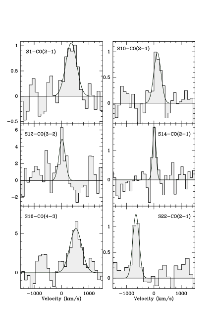
Figure 2: CO spectra of the detected galaxies. Zero velocity corresponds to the optically determined redshift, listed in Table 1. According to the redshift, the lowest frequency observable is either the CO(2-1) or CO(3-2) line. One source (S16) is detected in CO(4–3) but not in CO(2-1), as indicated in Table 2. The vertical scale is T_mb in mK.

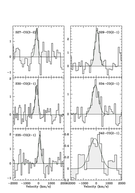
Figure 3: Same as Fig. 2 for additional galaxies.

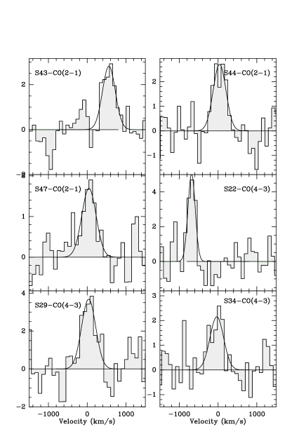
Figure 4: Same as Fig. 2 for the remaining 3 galaxies. The final 3 plots are CO(4-3) spectra from some sources already shown in CO(2-1).

The majority of the sources have IRAS fluxes at 60 and 100$\mu$m, and their far-infrared fluxes F_FIR are computed as 1.26 x 10^-14 (2.58 S₆₀+S₁₀₀) W m^-2 (Sanders & Mirabel 1996). The far-infrared luminosity between 40 and 500$\mu$m is then L_FIR = 4 $\pi$ D${}_{L}^{2}$ CC F_FIR, where D_L is the luminosity distance, and CC the color correction, CC=1.42. Some of the sources instead have Spitzer-MIPS fluxes at 70 and 160$\mu$m. We chose to compute their F_FIR fluxes similarly, with a linear combination of these two fluxes, since all sources are ultraluminous objects; i.e., their SEDs fall into the same category, and this gives comparable results to those of SED fitting (e.g. Symeonidis et al. 2008). The FIR-to-radio ratio $q$=log([F_FIR/(3.75 10¹² Hz)]/[f_ν(1.4 GHz)]) has been computed for sources where radio data are available; the radio fluxes are listed in Table 2. If excluding the radio galaxies 3C280 and 3C289 (S18 and S20), the average is $q$=1.7, close to the nominal value for ULIRGs (Sanders & Mirabel 1996). The SFRs are all above 200 $\rm M_{\odot}yr^{-1}$, and the sample average is 1200 $\rm M_{\odot}yr^{-1}$, as estimated from the infrared luminosity (e.g. Kennicutt 1998).

In this article, we adopt a standard flat cosmological model, with $\Lambda$ = 0.73, and a Hubble constant of 71 km s^-1 Mpc^-1 (Hinshaw et al. 2009).

Table 1: Definition of the sample, selected by FIR luminosity

S	Source	RA(2000)	DEC(2000)	z
S1	aJ005009.81-003900.5	00:50:09.8	-00:39:01	0.727
S2	FF J0139+0115	01:39:27.4	+01:15:52	0.612
S3	IRAS Z02317-0152	02:34:21.8	-01:39:01	0.645
S4	aJ014612.79+005112.4	01:46:12.8	00:51:12	0.622
S5	IRAS Z02433+0110	02:45:55.5	+01:23:29	0.798
S8	aJ080430.99+360718.1	08:04:31.0	+36:07:18	0.656
S9	aJ081929.48+522345.2	08:19:29.5	+52:23:45	0.624
S10	aJ084846.34+022034.1	08:48:46.3	+02:20:34	0.627
S11	aJ091501.71+241812.1	09:15:01.7	+24:18:12	0.840
S12	aJ092527.80+001837.1	09:25:27.8	+00:18:37	0.812
S13	aJ093741.65+385752.6	09:37:41.6	+38:57:53	0.621
S14	IRAS F10398+3247	10:42:40.8	+32:31:31	0.633
S16	SBS 1148+549	11:51:20.4	+54:37:33	0.975
S18	3C 280	12:56:57.1	+47:20:20	0.996
S20	3C 289	13:45:26.4	+49:46:33	0.967
S21	aJ144642.28+011303.0	14:46:42.3	+01:13:03	0.725
S22	aJ144953.69+444150.3	14:49:53.7	+44:41:50	0.670
S23	IRAS F14537+1950	14:56:04.4	+19:38:46	0.640
S25	aJ153244.01+324246.6	15:32:44.0	+32:42:47	0.926
S26	aJ160222.38+164353.7	16:02:22.4	+16:43:54	0.672
S27	aJ160825.24+543809.8	16:08:25.2	+54:38:10	0.907
S28	CFN1 078	16:12:37.0	+54:28:51	0.910
S29	aJ161422.14+323403.6	16:14:22.1	+32:34:04	0.710
S30	aJ172507.39+370932.1	17:25:07.4	+37:09:32	0.689
S32	IRAS 17548+6706	17:54:49.6	+67:05:57	0.919
S34	IRAS Z21293-0154	21:31:53.5	-01:41:43	0.730
S35	PG 0044+030	00:47:05.9	+03:19:55	0.623
S36	bEGS70-158	14:21:37.5	+53:17:18	0.930
S37	bEGS70-124	14:22:39.2	+53:24:21	0.850
S38	aJ142301.15+532419.2	14:23:01.1	+53:24:19	0.660
S39	aJ142348.80+533006.3	14:23:48.8	+53:30:06	0.770
S40	bEGS70-067	14:24:30.1	+53:35:43	0.960
S41	bEGS70-058	14:25:02.8	+53:31:25	0.690
S42	aJ143047.32+602304.4	14:30:47.3	+60:23:04	0.607
S43	aJ143151.84+324327.9	14:31:51.8	+32:43:28	0.660
S44	aJ143820.76+340234.3	14:38:20.7	+34:02:34	0.670
S45	aJ172228.04+601526.0	17:22:28.0	+60:15:26	0.742
S46	aJ171302.41+593611.1	17:13:02.4	+59:36:11	0.668
S47	aJ171312.08+600840.4	17:13:12.0	+60:08:40	0.759

[^a] SDSS source; [^b] [SWR2008]. Redshifts are taken from the NED data base.

3 Observations

The observations were carried out with the IRAM 30m telescope at Pico Veleta, Spain, in two periods, January and June 2011, with a few remaining sources observed in the pool between November 2011 and February 2012. According to their redshifts, sources were observed in their CO(2-1), CO(3-2) or CO(4-3) lines, either with the 3mm, 2mm or 1mm receivers. Often only one line was observable. When possible and when the atmosphere was favorable, we simultaneously observed two CO lines. This was possible for seven galaxies (see Table 2).

The broadband EMIR receivers were tuned in single sideband mode, with a total bandwidth of 4 GHz per polarization. This covers a velocity range of $\sim$ 12,000  km s^-1at 3mm and $\sim$ 8,000  km s^-1at 2mm. The observations were carried out in wobbler switching mode, with reference positions offset by $2\arcmin$ in azimuth. Several backends were used in parallel, the WILMA autocorrelator with $2$ MHz channel width, covering 4$\times$4 GHz, and the $4$ MHz filterbanks, covering 2$\times$4 GHz.

We spent on average three hours on each galaxy, and reached a noise level between 0.7 and 2 mK (main beam temperature), smoothed over $30$ km s^-1 channels for all sources. Pointing measurements were carried out every two hours on continuum sources and the derived pointing accuracy was 3^′′ rms. The temperature scale used is main beam temperature $T_{\rm mb}$. At 3mm, 2mm and 1mm, the telescope half-power beam width is 27^′′, 17^′′ and 10^′′, respectively. The main-beam efficiencies are $\eta$${}_{\rm mb}=T_{\rm A}^{*}/T_{\rm mb}$=0.85, 0.79 and 0.67, respectively, and $S/T_{\rm mb}$ = 5.0 Jy/K for all bands. Spectra were reduced with the CLASS/GILDAS software, and the spectra were smoothed up to $\sim 60$ km s^-1 channels for the plots.

Table 2: Observed line parameters

Gal	Line	$\nu_{\rm obs}$	S(CO)a	$V^{b}$	$\Delta V_{\rm FWHM}$	L’CO/1010	S60	S${}_{100}^{c}$	log LFIR	F(1.4GHz)d	log M${}_{*}^{f}$
		[GHz]	[Jy  km s-1]	[ km s-1]	[ km s-1]	[K  km s-1  pc2]	[Jy]	[Jy]	[L⊙]	[mJy]	[M⊙]
S1	CO(21)	133.490	2.1 $\pm$ 0.3	354. $\pm$ 37.	469. $\pm$ 73.	1.53	0.26	0.44	13.09	4.3	10.84g
	CO(43)	266.960	4.1 $\pm$ 1.1	428. $\pm$ 96.	702. $\pm$ 208.	0.74
S2	CO(21)	143.014	$<$ 1.2			$<$ 0.6	0.23	0.21	12.77	9.0	10.58
S3	CO(21)	140.145	$<$ 1.0			$<$ 0.6	0.14	0.03	12.51	70.3	9.58
S4	CO(43)	284.242	$<$ 1.0			$<$ 0.1	0.06	$<$0.12	12.32	–	11.55
S5	CO(43)	256.419	$<$ 3.0			$<$ 0.7	0.21	0.40	13.12	2.0	10.84g
S8	CO(21)	139.196	$<$ 1.2			$<$ 0.7	0.03	0.36	12.58	73.7	10.71
S9	CO(21)	141.957	$<$ 1.0			$<$ 0.5	0.25	0.03	12.72	2.6	10.20
S10	CO(21)	141.698	1.3 $\pm$ 0.2	132. $\pm$ 27.	291. $\pm$ 64.	0.68	0.15	0.03	12.51	1.1	10.59
S11	CO(43)	250.566	$<$ 4.1			$<$ 1.0	0.25	0.03	13.03	9.3	11.01h
S12	CO(32)	190.837	4.8 $\pm$ 1.4	20. $\pm$ 36.	271. $\pm$ 102.	1.93	0.15	0.03	12.79	–	10.42
S13	CO(21)	142.220	$<$ 0.8			$<$ 0.4	0.22	0.32	12.83	0.7	11.43
S14	CO(21)	141.175	1.1 $\pm$ 0.2	1. $\pm$ 15.	122. $\pm$ 29.	0.61	0.22	0.54	12.94	6.3	10.62
	CO(43)	282.327	3.7 $\pm$ 0.9	-82. $\pm$ 65.	493. $\pm$ 99.	0.49
S16	CO(21)	116.704	$<$ 3.2			$<$ 4.2	0.20	0.41	13.33	4.5	12.66gh
	CO(43)	233.389	10.3 $\pm$ 1.6	521. $\pm$ 31.	483. $\pm$ 103.	3.36
S18	CO(43)	230.982	$<$ 2.0			$<$ 0.7	0.12	0.06	12.95	5100.0	10.33
S20	CO(43)	234.340	$<$ 1.8			$<$ 0.6	0.10	0.03	12.82	2400.0	11.66g
S21	CO(21)	133.614	$<$ 0.8			$<$ 0.6	0.08	0.15	12.60	5.9	11.54
S22	CO(21)	138.047	1.8 $\pm$ 0.4	-656. $\pm$ 25.	249. $\pm$ 57.	1.11	0.19	0.03	12.68	11.0	10.04
	CO(43)	276.072	6.0 $\pm$ 0.9	-685. $\pm$ 16.	214. $\pm$ 33.	0.91
S23	CO(21)	140.572	$<$ 1.0			$<$ 0.6	0.28	0.03	12.79	–	10.29
S25	CO(43)	239.415	$<$ 3.0			$<$ 0.9	0.28	0.50	13.40	5.9	11.36g
S26	CO(21)	137.882	$<$ 1.2			$<$ 0.7	0.15	0.03	12.59	1.9	11.85h
S27	CO(32)	181.330	1.5 $\pm$ 0.3	-128. $\pm$ 28.	211. $\pm$ 60.	0.77	0.03	0.26	12.82	0.2	11.25
S28	CO(43)	241.383	$<$ 2.2			$<$ 0.6	0.03	0.24	12.80	–	10.14
S29	CO(21)	134.818	4.4 $\pm$ 0.5	68. $\pm$ 18.	373. $\pm$ 48.	3.02	0.17	0.21	12.84	1.2	11.39g
	CO(43)	269.614	8.4 $\pm$ 1.6	40. $\pm$ 38.	421. $\pm$ 85.	1.43
S30	CO(21)	136.494	2.4 $\pm$ 0.4	-133. $\pm$ 21.	267. $\pm$ 43.	1.52	0.24	0.23	12.92	2.3	11.04g
	CO(43)	272.967	1.3 $\pm$ 0.4	-32. $\pm$ 6.	44. $\pm$ 26.	0.21
S32	CO(43)	240.251	$<$ 1.8			$<$ 0.5	0.40	0.47	13.48	–	10.72
S34	CO(21)	133.259	3.6 $\pm$ 0.5	-60. $\pm$ 41.	569. $\pm$ 96.	2.58	0.19	0.56	13.07	2.7	10.84g
	CO(43)	266.498	4.8 $\pm$ 1.1	-34. $\pm$ 52.	414. $\pm$ 104.	0.87
S35	CO(21)	142.022	1.8 $\pm$ 0.5	93. $\pm$ 19.	182. $\pm$ 70.	0.93	0.07	0.16	12.41	166.4	11.79h
S36	CO(43)	238.881	$<$ 3.6			$<$ 1.1	0.03e	0.14e	12.66	–	11.62
S37	CO(43)	249.211	$<$ 2.8			$<$ 0.7	0.01e	0.06e	12.21	–	11.29
S38	CO(21)	138.878	$<$ 1.4			$<$ 0.8	0.02e	0.08e	12.04	–	10.83
S39	CO(21)	130.247	$<$ 1.2			$<$ 1.0	0.01e	0.10e	12.25	–	12.19h
S40	CO(43)	235.225	$<$ 1.8			$<$ 0.6	0.01e	0.09e	12.42	–	11.69
S41	CO(21)	136.413	$<$ 1.0			$<$ 0.7	0.01e	0.12e	12.15	–	11.77
S42	CO(21)	143.472	2.3 $\pm$ 0.4	-98. $\pm$ 93.	1001. $\pm$ 244.	1.12	0.06	0.20	12.41	15.0	11.86
S43	CO(21)	138.878	4.7 $\pm$ 0.6	560. $\pm$ 23.	385. $\pm$ 49.	2.75	0.05e	0.14e	12.38	–	11.05g
S44	CO(21)	138.047	5.9 $\pm$ 1.0	60. $\pm$ 36.	415. $\pm$ 72.	3.59	0.07e	0.25e	12.57	–	11.38g
S45	CO(21)	132.345	$<$ 1.8			$<$ 1.4	0.04e	$<$0.15e	12.47	1.2	11.67
S46	CO(21)	138.212	$<$ 1.4			$<$ 0.9	0.04e	$<$0.16e	12.39	4.6	10.72
S47	CO(21)	131.030	3.1 $\pm$ 0.7	46. $\pm$ 46.	437. $\pm$ 153.	2.45	0.03e	$<$0.11e	12.34	0.5	11.31

• Quoted errors are statistical errors from Gaussian fits. The systematic calibration uncertainty is 10%.

• The derivation of L_FIR is described in Sec. 2, and log SFR(M_⊙/yr) = log L_FIR(L_⊙) - 9.76 (cf Sec.4.2).

• The upper limits are at 3$\sigma$ with an assumed $\Delta$V = 300  km s^-1, except for S16, where $\Delta$V is known.

• The velocity is relative to the optical redshift given in Table 1.

• The 60 and 100$\mu$m  fluxes are from NED (http://nedwww.ipac.caltech.edu/) or Stanford et al. (2000)

• From the FIRST catalog (http://sundog.stsci.edu/). Errors are typically 0.14 mJy

• For these objects, the Spitzer 70 and 160$\mu$m fluxes replace the IRAS 60 and 100$\mu$m ones.

• Stellar masses were obtained through SED fitting (see Sec. 4.6), with SDSS fluxes for all galaxies, and in addition, with Spitzer-IRAC data for galaxies with [^g] and 2MASS for galaxies with [^h] in the last column.

4 Results

4.1 CO detection in z=0.6-1.0 ULIRGs

Figures 2, 3 and 4 display the CO-detected sources, in their lower-J CO spectrum. For three galaxies, S22, S29 and S34, their higher-J lines are also plotted. Table 2 reports all line parameters, and also the upper limits for the non detections. Integrated signals and velocity widths have been computed from Gaussian fits. These also give the central velocities, with respect to the optical redshift of Table 1. There are some offsets between the CO and optical velocities, always lower than 700 km s^-1. These offsets might be due to the accuracy of the optical determination, or be intrinsic due to an outflow of ionized gas. The upper limits are computed at 3$\sigma$, assuming a common line width of 300 km s^-1and getting the rms of the signal over 300 km s^-1. Lines are considered detected when the integrated signal is more than 3$\sigma$. All spectra above 3$\sigma$ are shown in the figures.

The detection rate of 38% in this z=0.6–1 sample is lower than the value of 60% found in the lower-z counterpart at z=0.2-0.6 (Paper II); however, this can already be explained by the reduced sensitivity for the more distant objects. Indeed, the lines detected are now CO(2-1) instead of CO(1-0), and for excited point sources the flux could be up to about four times larger; however, the average luminosity distance at 0.6 $<$ z $<$ 1.0 weakens the signal by about a factor 5.5 with respect to the previous closer sample, and this outweighs the gain by climbing up the CO ladder. At 0.6 $<$ z $<$ 1.0, the average angular distance is 1550 Mpc; i.e., the beam of 17^′′ corresponds to 127 kpc, so the sources can all be considered as point-like at this resolution.

The line widths detected are compatible with what is expected from massive galaxies of ULIRG type, and quite comparable to what was found in our lower-z sample. Their average is $\Delta$V_FWHM= 370  km s^-1, compared to 348 km s^-1 in Paper II. Some galaxies have somewhat different widths in their two detected CO lines, but this is likely due to the noise intrinsic to the data.

4.2 CO luminosity and H₂  mass

Since we have not observed the fundamental CO(1-0) line, which is a direct measure of the total H₂  mass, but mostly CO(2-1), it is interesting to compute L’_CO, the special unit CO luminosity, through integrating the CO intensity over the velocity profile. This luminosity, expressed in units of K  km s^-1pc², will give the same value irrespective of J, if the CO lines are saturated and have the same brightness temperature.

This CO luminosity is given by

$$L^{\prime}_{CO}=23.5I_{CO}\Omega_{B}{{D_{L}^{2}}\over{(1+z)^{3}}}\hskip 6.0pt\rm{K\hskip 3.0ptkm\hskip 3.0pts^{-1}\hskip 3.0ptpc^{2}}$$

where $I_{CO}$ is the intensity in K  km s^-1, $\Omega_{B}$ the area of the main beam in square arcseconds, and $D_{L}$ the luminosity distance in Mpc. As mentioned above, all sources can be considered to be unresolved, since our beam is typically 130kpc in size. We here assume a ratio of 1 between the CO(2-1) and CO(1-0) luminosities (or brightness temperatures), as expected for a warm optically thick, and thermally excited medium. In Paper II, we found some sources with lower excitation, but the excitation appears higher in the present sample, as discussed in section 4.3. In any case, our hypothesis of a CO(2-1)/CO(1-0) ratio equal to unity can only underestimate the CO(1-0) luminosity and thus the molecular masses. Under this assumption, we compute H₂ masses using M${}_{\rm H_{2}}=\alpha$ L’_CO, with $\alpha=0.8$ M_⊙ (K  km s^-1  pc²)^-1, the appropriate factor for ULIRGs. The molecular gas masses are listed in Table 3. The choice of a common conversion factor might not be realistic, but it is a first approximation before knowing more physical quantities about each source, and adapting an individual factor for each, based on observation of more CO lines and of the gas spatial extent. In the following, CO luminosities are often used instead of H₂ masses, to remind the reader of this uncertainty.

The average CO luminosity for the 15 galaxies detected is L’_CO = 1.8 10¹⁰ K  km s^-1  pc², corresponding to an average H₂  mass of 1.5 10¹⁰ M_⊙. The star formation efficiency (SFE), also listed in Table 3, is defined as L_FIR/M(H₂) in L_⊙/M_⊙. The SFR is related to the FIR luminosity, where we adopt the relation SFR= L_FIR /(5.8 10⁹L_⊙) compiled by Kennicutt (1998). The gas consumption time scale can then be derived as $\tau$ = 5.8/SFE Gyr, where SFE is in units of L_⊙/M_⊙.

Table 3: Molecular gas mass, star formation efficiency, dust temperature and dust mass, half-light radius and galaxy type of the sample

S	M(H2)	SFE	Td	Md	R1/2	Type
	109 M⊙	L⊙/M⊙	K	108 M⊙	kpc
S 1	12.3	1003.	58.7	1.4	1.1a	S2,Q,wi
S 2	$<$4.9	$>$1205.	70.1	0.3	2.9a	wi
S 3	$<$4.5	$>$713.	66.5	0.2	0.5a
S 4	$<$1.1	$>$1978.	$>$ 52.0	$<$0.5	3.9	S2,Q,si
S 5	$<$5.3	$>$2504.	58.6	1.6	3.1a	si
S 8	$<$5.6	$>$674.	33.4	20.7	7.3	S2,Q
S 9	$<$4.2	$>$1238.	68.2	0.3	4.2	S1
S10	5.4	597.	67.7	0.2	8.5	S2
S11	$<$7.8	$>$1375.	76.0	0.4	1.1a	Q,si
S12	15.4	400.	75.4	0.2	5.0	S2
S13	$<$3.4	$>$2012.	58.2	0.8	2.2a
S14	4.9	1776.	49.0	3.0	0.9a	si
S16	21.0	1016.	62.4	1.8	2.9a	Q
S18	$<$5.5	$>$1624.	81.0	0.2	3.4a
S20	$<$4.7	$>$1419.	69.0	0.4	3.3a	si
S21	$<$4.6	$>$861.	56.5	0.6	6.4	S2,Q
S22	8.8	541.	77.2	0.2	1.5a	S2
S23	$<$4.5	$>$ 1381.	72.2	0.3	3.5
S25	$<$7.1	$>$3536.	64.2	1.8	1.3a	S2,si
S26	$<$5.9	$>$656.	70.2	0.2	6.2	wi
S27	6.2	1070.	41.3	9.4	7.9
S28	$<$5.0	$>$1254.	42.2	7.7	–
S29	24.1	286.	65.4	0.4	1.6a	si
S30	12.2	683.	71.8	0.3	1.1a	wi
S32	$<$4.2	$>$7190.	74.8	0.9	4.0
S34	20.7	569.	49.1	4.2	7.8a	si
S35	7.4	346.	50.0	0.8	2.8a	S2,Q,wi
S36	$<$8.6	$>$ 531.	35.1	18.6	6.4
S37	$<$5.6	$>$ 284.	34.2	7.0	–
S38	$<$6.7	$>$ 161.	30.4	9.1	2.2	wi
S39	$<$7.8	$>$222.	29.9	23.5	11.	wi
S40	$<$4.6	$>$574.	33.1	20.5	–
S41	$<$5.2	$>$265.	26.3	55.6	–
S42	8.9	287.	44.0	1.7	7.8	Q,si
S43	22.0	109.	34.1	6.9	5.6	wi
S44	28.7	129.	31.9	21.1	5.6	wi
S45	$<$10.9	$>$265.	$>$32.8	$<$14.8	4.0	si
S46	$<$6.8	$>$343.	$>$31.3	$<$15.8	5.5
S47	19.6	112.	$>$33.1	$<$10.9	3.1a	si

M(H₂) and SFE are defined in Sec. 4.8, T_d and M_d in Sec. 4.5
R_1/2 is defined from red images either from SDSS, or HST for the galaxies with index [^a]
The latter images were used to determine the morphological class: wi, si= weak & strong interaction. The nuclear activity type is derived from NED: S1, S2= Seyfert 1 & 2, Q= QSO

4.3 Molecular gas excitation

Seven sources have been observed in two CO lines, CO(2-1) and CO(4-3), and six have been detected in both, as listed in Table 4. One has an upper limit, in the CO(2-1) line. To compare the two lines, and derive the excitation, we computed both the total and the peak flux ratio S₄₃/S₂₁ since the CO(4-3) and CO(2-1) lines have sometimes different measured linewidths, which we attribute to noise. The corresponding ratios between the peak brightness temperatures are also displayed in Table 4, to allow for easy comparison with the predictions of excitation models. The temperature ratio is corrected for the different beam sizes, assuming that the sources are unresolved in all our observations.

The excitation essentially depends on two parameters, the H₂  volume density, and the kinetic temperature. In ultraluminous objects, the column densities of the molecular gas are high enough (N(H₂) $>$ 10²⁴ cm^-2) that the CO lines are always optically thick in the low-J lines. This result was reached through mapping the gas content of local ULIRGs, where the gas is very concentrated (e.g. Solomon et al. 1997). Depending on the velocity width of the lines, the CO column density per unit velocity width (km/s) is higher than 10¹⁷ cm^-2. To constrain the kinetic temperature of the gas, we computed the dust temperature deduced from the far-infrared fluxes (see Table 3), assuming $\kappa_{\nu}\propto\nu^{\beta}$, where $\kappa_{\nu}$ is the mass opacity of the dust at frequency $\nu$, and $\beta$ = 1.5. The average dust temperature for our 0.6$<$z$<$1.0 sample is $54\pm 5$ K, higher than the average dust temperature for the 0.2$<$z$<$0.6 sample of $46\pm 5$ K (Paper II). This is also higher than what is obtained for local starburst galaxies, which have dust temperatures $\approx 40$ K (e.g. Sanders & Mirabel 1996, Elbaz et al. 2010). Yang et al. (2007) have observed seven of our objects at 350$\mu$m and derive more precise temperatures, which are very similar to the values computed above. We note a clear increase in the dust temperatures with respect to our 0.2 $<$ z $<$ 0.6 sample in Paper II. This could be caused by selection effects, and also be due to the frequency used to measure the temperature. The 60 and 100$\mu$m bands correspond to rest-frame 45 and 76$\mu$m at z$\sim$ 0.32, and to rest-frame 35 and 58$\mu$m at z$\sim$ 0.72, the median redshift of the two samples.

As in Paper II, we assume that the gas is predominantly heated by collisions with the dust grains. Indeed, there could be small regions that are heated by the UV photons of young massive stars or by shocks, but our beam encompasses kpc scales, and these would be spatially diluted. The gas kinetic temperature should be at most equal to the dust temperature, and this is the constraint used in our LVG modeling. We compare the CO-based molecular masses and dust masses in section 4.5.

Using the Radex code (van der Tak et al. 2007), we computed the predicted main beam temperature ratio between the CO(4-3) and CO(2-1) lines, for several kinetic temperatures and as a function of H₂  densities, and CO column densities. Figure 5 shows these predictions for T_k=60 K and 30 K. The black contours delineate the range of observed values. In Table 4 we list the derived values for the n(H₂) densities, for two values of the kinetic temperatures (60 and 30K), and for a fixed column density per velocity width.

We adopted a column density of N(CO)/$\Delta V$ of 7$\times$10¹⁶ cm^-2/( km s^-1), which corresponds to what is expected if the high molecular gas masses derived in Table 2 are highly concentrated in the few central kpc. For M(H₂) = 3 10¹⁰ M_⊙, a typical CO abundance of CO/H₂  = 10^-4, and a linewidth of 300  km s^-1, this column density corresponds to a homogenous disk of 3 kpc in size. This average column density would be a lower limit, if the gas inside 3kpc is clumpy.

The excitation of the CO gas is in general higher than in our lower-z sample. In Paper II, the CO(3-2)/CO(1-0) ratio was found to be $\sim$ 3 times lower than the CO(4-3)/CO(2-1) ratio derived here, and the H₂  volumic densities were on the order of 100, while they are $\sim$ 10³ cm^-3 in the present analysis. In four out of the seven sources where we have excitation constraints through measurements of two lines, the CO emission ladder should be populated well above the J=4 line. In the three remaining sources, the excitation is typical of “normal” or weakly interacting galaxies, like the Milky Way or the Antennae (e.g. Weiss et al. 2007).

We note that these conclusions on the excitation are preliminary. Observations of several lines for more sources are required, as there are large variations from source to source. In addition, the spatial extent of the emission needs to be obtained through interferometric measurements.

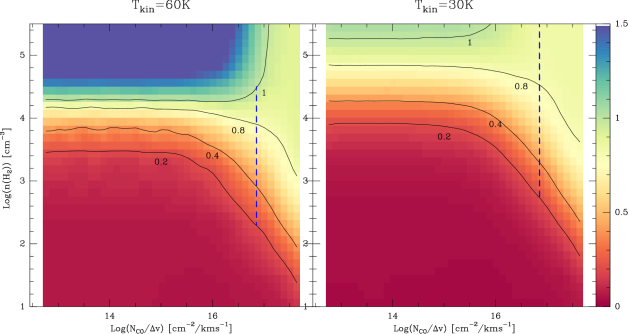
Figure 5: Peak T_b ratio between the CO(4-3) and CO(2-1) lines versus H₂  density, and the CO column density per unit velocity width (N${}_{\rm CO}/\Delta V$) for two values of the kinetic temperature: T_k = 60K, the dust temperature (left), and T_k = 30K (right). The black contours are underlining the values obtained in the data. In both panels, the vertical line corresponding to (N${}_{\rm CO}/\Delta V$)= 7$\times$10¹⁶ cm^-2/( km s^-1), value chosen in Table 4, has been emphasized with blue dashes. The predictions come from the LVG models that are part of the Radex code (van der Tak 2007).

4.4 CO luminosity and redshift

As in Paper II, we can now investigate the evolution of the molecular gas content of galaxies with redshift. The CO luminosity of our sample objects, selected to be bright with high masses, is now compared to data reported in the literature at different redshifts, also selected with high masses, in Figure 6. The local sample is the compilation of 65 infrared galaxies by Gao & Solomon (2004), including nine ULIRGs (L${}_{\rm FIR}>$10¹²L_⊙), 22 luminous infrared galaxies LIGs (10¹¹L_⊙$<$L${}_{\rm FIR}<$10¹²L_⊙), and 34 large spiral galaxies. We include 37 ULIRGs from the study by Solomon et al. (1997) up to z=0.3, and 29 ULIRGs from Chung et al. (2009) up to z=0.1. At intermediate redshift of 0.4, we include five massive star-forming galaxies selected at 24$\mu$m, and detected by Geach et al. (2009, 2011). They are compared with the compilation by Iono et al. (2009) of 43 low and high-redshift U/LIRGs, submm selected galaxies (SMGs), quasars, and Lyman Break Galaxies (LBGs), 19 high-z SMG from Greve et al. (2005), massive star-forming galaxies at high-z from Daddi et al. (2010), Genzel et al. (2010) and Solomon & van den Bout (2005). Our full sample (filled black circles, Paper II and this work) now fills in the CO redshift desert, between z=0.2 and 1. The average CO luminosity over our 33 detected galaxies is L’_CO = 1.9$\times$10¹⁰ K  km s^-1  pc², while the average over the local star-forming galaxies (Gao & Solomon 2004) is 0.36$\times$10¹⁰ K  km s^-1  pc², a factor 5 lower. It has been already established that galaxies have more molecular gas at high redshift, z $\sim$ 1-2 (Tacconi et al. 2010, Daddi et al. 2010), while the abundance of HI is not thought to have varied significantly since z = 1.5 (e.g. Obreschkow & Rawlings 2009). Now it is possible to determine that the rise is gradual, and it already starts at z=0.2-0.3. This trend is also discussed for the gas fraction (M_gas/(M_gas+M_∗) in Section 4.6.

Obviously, such a trend is only indicative and should be confirmed by the study of a large number of galaxies in the main sequence of star formation, and by sampling a larger part of the luminosity function. Here we focus on the most luminous objects, and the evolution we observed is only that of most actively starforming galaxies. We expect that this evolution in L’_CO probably underestimates the evolution in molecular mass: at higher z, the CO luminosity has been measured in higher-J lines, and because of likely subthermal excitation, those lines must have lower luminosity than the CO(1-0) line.

Theoretically, it is expected that galaxies are richer in molecular gas at high redshift. Indeed, galaxies at a given mass should be smaller (Somerville et al. 2008), which is confirmed by observations (e.g. Nagy et al. 2011). As a consequence, the gas component was more compact and thus denser, and the higher gas pressure transforms the HI into a molecular gas phase, increasing the H₂/H I  ratio. Since the abundance of HI is not predicted to vary significantly since z=1.5, the H₂/H I  ratio reflects the evolution of the molecular gas content, traced by CO luminosity. Obreschkow et al. (2009) and Obreschkow & Rawlings (2009) followed the H₂/H I  ratio statistically over 30 million simulated galaxies, and predicted its cosmic decline as $\Omega_{{\rm H}_{2}}$/$\Omega_{{\rm H}{\rm\small I}}\propto(1+z)^{1.6}$. To guide the eye, we have reproduced this behavior through a red line in Figure 6. The amplitude of variation in the L’_CO envelope appears to approximately follow the line.

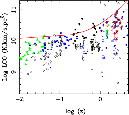
Figure 6: Measured CO luminosities, corrected for amplification when known, but not for gas excitation, as a function of redshift. We compare our points (filled black circles, and arrows as upper limits) with a compilation of high-z molecular gas surveys, and local ones: green filled triangles are from Gao & Solomon (2004), filled blue squares from Solomon et al. (1997), open circles from Chung et al. (2009), open blue diamonds from Geach et al. (2009, 2011), black crosses from Iono et al. (2009), red stars from Greve et al. (2005), green filled circles from Daddi et al. (2010), blue asterisks from Genzel et al. (2010), and blue filled circles from Solomon & vanden Bout (2005). For illustration purposes only, the red curve is the power law in (1+z)^1.6 for $\Omega_{{\rm H}_{2}}$/$\Omega_{{\rm H}{\rm\small I}}$ proposed by Obreschkow & Rawlings (2009).

4.5 Correlation between FIR and CO luminosities

It is now well-known that a good correlation exists between FIR and CO luminosities (e.g. Young & Scoville 1991). It holds for star-forming galaxies, either in the main sequence or in the starbursting phase, and even for quasars, implying that their FIR luminosity is dominated by star formation (Iono et al. 2009, Xia et al. 2012). The correlation is slightly non linear, and Xia et al. (2012) found a power law of slope 1.4 as their best-fit, which is confirmed in Figure 7: this means that ultra-luminous sources are forming stars at higher efficiency, and with a depletion time as low as $\sim$ 10 Myr.

In Figure 7, we draw three lines corresponding to three orders of magnitude of the ratio L_FIR/M(H₂), if the CO-to-H₂  conversion factor adapted for ULIRG is used. Within this hypothesis, all galaxies in our sample are located above the curve L_FIR/M(H₂)=100 L_⊙/M_⊙  (corresponding to a consumption time scale of $\tau$ =58 Myr). However, all detected galaxies at high z in the literature are also in this regime, including the main-sequence star-forming galaxies at high redshift studied by Genzel et al. (2010) or Daddi et al. (2010). In those objects, gas excitation and spatial extent argue in favor of a more “normal” conversion factor, as for the Milky Way. If we adopt a MW-like conversion factor, the H₂  mass then moves to the right by a factor 5.75 (or 0.76 in log), and these objects will fall in the range of L_FIR/M(H₂) between 10 and 100 L_⊙/M_⊙  with a depletion time scale approaching the Gyr. In such conditions, star formation could be sustained continuously, given the frequent cold gas accretion from the intergalactic medium.

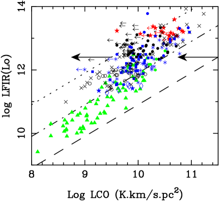
Figure 7: Correlation between FIR and CO luminosities, for our sample (filled black circles, and arrows for upper limits) and other galaxies from the literature (same symbols as in Fig 6). The 3 lines are for L_FIR/M(H₂)=10, 100 and 1000 L_⊙/M_⊙  from bottom to top, assuming a conversion factor $\alpha$ = 0.8 M_⊙ (K  km s^-1  pc²)^-1. The same lines correspond to gas depletion time scales of 580 (bottom), 58 (middle) and 5.8 Myr (top). The arrows indicate the direction and amount by which these lines would move if the Milky Way CO-to-H₂  conversion factor was used.

To better constrain the correct conversion factor to apply to each object, we derive the dust mass from the far-infrared measurements, and compare it with the gas mass. Given the already derived dust temperature T_d and the observed 100 $\mu$m  flux S₁₀₀, we can estimate the dust mass as

$$\begin{array}[]{lcl}{\rm M}_{d}&=&4.8\times 10^{-11}\,{{S_{\nu o}\,D_{\rm Mpc}^{\,2}}\over{(1+z)\kappa_{\nu r}\,B_{\nu r}(T_{d})}}\ {{\rm M}_{\odot}}\\ &=&5(1+z)^{-(4+\beta)}\,S_{100\mu{\rm m}}\,D_{\rm Mpc}^{\,2}\,\left\{\exp(144(1+z)/T_{d})-1\right\}\ {{\rm M}_{\odot}}\\ \end{array}$$

where $S_{\nu o}$ is the observed FIR flux measured in Jy, $D_{\rm Mpc}^{\,2}$ the luminosity distance in Mpc, $B_{\nu r}$ the Planck function at the rest frequency $\nu r=\nu o(1+z)$, and we use a mass opacity coefficient of $25$ cm² g^-1 at rest frame 100 $\mu$m (Hildebrand 1983, Dunne et al. 2000, Draine 2003), with a frequency dependence of $\beta$=1.5. Estimated dust masses are displayed in Table 3. If we adopt the low conversion factor of $\alpha$ = 0.8 M_⊙ (K  km s^-1  pc²)^-1, the average gas-to-dust mass ratio is 206 for the detected galaxies. The gas-to-dust mass ratio would increase up to 1200 if the standard (MW) conversion factor is used. Since the Milky Way gas-to-dust ratio is 150, which is also a value typically found in nearby galaxies in the SINGS sample (Draine et al. 2007), while values higher than 1000 are only found in elliptical galaxies, or in low-metallicity dwarfs (Wiklind et al. 1995, Leroy et al. 2011), we conclude that the ULIRG conversion factor is not far from being adequate for our sample. We note that for the high stellar masses of the sample galaxies, when using the mass metallicity relation, and its evolution by a factor 2-3 with redshift up to z=0.75 (Moustakas et al. 2012), we could expect an average gas-to-dust mass ratio of no more than 500 for our sample.

Table 4: CO gas excitation

S	S43/S21	S43/S21	Tb43/Tb21	n(H2)	n(H2)
	[total]	[peak]	[peak]	[cm-3]	[cm-3]
				60K	30K
S1	2.0	1.3 $\pm$ 0.3	0.3 $\pm$ 0.07	4.E2	1.2E3
S14	3.4	1.0 $\pm$ 0.3	0.25 $\pm$ 0.07	3.E2	1.E3
S16	$>$3.2	$>$3.0	$>$ 0.75	$>$6.E3	$>$2.E4
S22	3.3	3.9 $\pm$ 0.8	1.0 $\pm$ 0.2	2.5E4	1.E6
S29	1.9	1.7 $\pm$ 0.3	0.4 $\pm$ 0.07	1.E3	2.E3
S30	0.5	3.2 $\pm$ 1.0	0.8 $\pm$ 0.2	8.E3	3.E4
S34	1.3	1.8 $\pm$ 0.4	0.4 $\pm$ 0.1	1.E3	2.E3

The gas excitation is discussed in Sec 4.3, n(H₂) is given for T_k=60K and 30K, and N${}_{\rm CO}/\Delta V$=7$\times$10¹⁶ cm^-2/( km s^-1)

4.6 Stellar mass and gas fraction

The redshift evolution of the CO luminosity envelope found in section 4.4 suggests that the declining gas content of galaxies could be an important driver of the decline in the cosmic star formation density since z=1. To better quantify this, we now measure the gas fraction of all systems at different redshifts, and estimate their stellar masses.

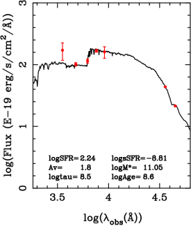
Figure 8: Spectral energy distribution (SED) of S43 (shown here as a representative example), based on optical/near-IR broadband photometry. The red points with error bars represent the observations of SDSS (ugriz bands), and of Spitzer/IRAC 3.6 and 4.5$\mu$m observations. The black curve is the overplotted best-fit stellar synthesis model, obtained with the FAST code (see text). An exponential star-formation history, where time scale tau is assumed, with a Salpeter IMF. Values for tau and population age are given in yr, as well as stellar mass (M_⊙), visual extinction (mag) SFR (M_⊙/yr), or specific SFR (yr^-1). All values are in log, except A_v.

To compute stellar masses from observed optical and near infrared (NIR) magnitudes, standard relations exist as a function of colors, derived from stellar populations models (see e.g. Bell et al. 2003). We used them for the local z=0 galaxies. For higher redshift objects, K-corrections need to be applied, and we used the analytical approximations from Chilingarian et al. (2010) in Paper II. However, for z$>$0.5, these are no longer valid, and for the present sample we estimated the stellar mass from SED-fitting of the optical and near-infrared luminosities taken from public catalogs, mainly the SDSS, 2MASS and Spitzer/IRAC fluxes. Most galaxies have only SDSS-DR8 fluxes, but ten have in addition 2MASS photometry, and another ten have Spitzer-IRAC fluxes. The broadband photometry were fitted using the code FAST (Fitting and Assessment of Synthetic Templates) described in Kriek et al. (2009). We selected the library of stellar population synthesis models of Bruzual & Charlot (2003), and adopted an exponential SFR $\propto$ exp(-t/tau), with a Salpeter initial mass function (IMF, Salpeter 1955). We used the extinction law by Calzetti et al. (2000), and metallicity was assumed to be solar. As for the IRAC fluxes, only the first two channels (3.6 and 4.5 $\mu$m) are relevant for the stellar component at the redshifts under consideration, so they were used for the fit. The visual extinction A_v was allowed to vary between 0 and 9, but the best fits were obtained for values always lower than three. The model fitting also gives an estimation of the SFRs, which frequently agrees within a factor 2-3 with what is derived from the far-infrared luminosities, except in a few cases (where it can be an order of magnitude different). The time scale for star formation is also derived, between the two limits that we set for the model fitting 10 Myr $<$ tau $<$ 300 Myr. We imposed the latter upper limit, to be consistent with the starburst nature of the objects. The parameters of the fit were selected such that the inverse of the specific SFR is always greater than tau. An example fit for the source S43 is presented in Figure 8. There is a certain degeneracy between the physical parameters, since the tau values are not tightly constrained; however, the stellar mass is more robust, depending on the SED fit and magnitudes observed. The derived masses are listed in Table 2.

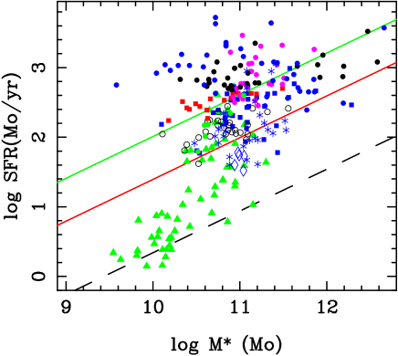
Figure 9: The star formation rate (SFR) obtained from the far infrared luminosity, versus stellar mass of galaxies in our sample (filled black circles for 0.2 $<$ z $<$ 0.6, and filled blue circles for 0.6 $<$ z $<$ 1.0), compared to the sample of Da Cunha et al. (2010, filled red squares), Fiolet et al. (2009, filled magenta circles), Gao & Solomon (2004, filled green triangles), Solomon et al. (1997, filled blue squares), Chung et al. (2009, open circles), Geach et al. (2009, 2011, blue diamonds), Daddi et al. (2010, filled green circles), and Genzel et al. (2010, blue asterisks). The black dashed line represents the star-forming galaxy main sequence at z=0, the red filled line the main sequence at z=1, and the green filled line the main sequence at z=2. All three lines have an adopted slope of 0.6 (Karim et al. (2011).

Stellar masses lie between 4$\times$10⁹ and 4$\times$10¹² M_⊙, with a median value of 1.1$\times$10¹¹ M_⊙. Figure 9 displays the SFR, derived from the infrared luminosity, versus stellar mass, in comparison with some other samples considered before, and adding the ULIRG samples of Da Cunha et al (2010) and Fiolet et al (2009). It is interesting to locate the position on the graph of the main sequence of star-forming galaxies, as defined by Noeske et al. (2007) and Daddi et al. (2007). We adopt the power laws of slope 0.6, and redshift evolution, as SFR$\propto$ M${}_{*}^{0.6}$(1+z)^3.5 as found by Karim et al. (2011). Our galaxy points sample the region significantly above the main sequence, with however some scatter, so that some galaxies reach the center of the main sequence. The star-forming galaxies at z=0, i.e. green triangles in Fig. 9 whose FIR luminosities are not all ULIRG, are also somewhat above the z=0 main sequence.

The gas fractions F_gas=MH₂/(M(H₂)+M_∗) derived from our stellar masses show large variations (see Figure 10). To obtain the gas fractions, we converted the CO luminosity to a gas mass using the ULIRG factor ($\alpha$=0.8). For the high-z samples, i.e. blue asterisks and green dots where the standard MW conversion has been selected by the authors, we extended in addition the points by a dotted line joining the two extreme values of gas fraction, obtained with $\alpha$=0.8 and 4.6 (the MW value). The gas fraction is well correlated with CO luminosity. The average gas fraction in our galaxies is 15% for the 0.2$<$z$<$0.4 sample, and 24% for the 0.6$<$z$<$1.0 sample. For the low-z samples by Gao & Solomon (2004), Solomon et al. (1997) and Chung et al. (2009), the averages are 5%, 6% and 7%, respectively, while they are 23% and 10% for the samples of Daddi et al. (2010) at z=1.5 and Genzel et al. (2010), at z=1-2. Assuming a standard MW conversion factor, the two last values become 63% and 35%. The increase in the gas fraction with z is clearly apparent, as shown in Figure 11. To guide the eye, we have indicated the z-evolution of the cosmic star formation history in this figure, as compiled by Hopkins & Beacom (2006), from different works in the literature, and complemented at very high redshift by the gamma-ray burst (GRB) data of Kistler et al. (2009) and the optical data (LBG) from Bouwens et al. (2008). In this approximate comparison, it is interesting to note that the rise in the SFR has only slightly higher amplitude than the rise of gas fraction, supporting the hypothesis of the large role of the gas in this evolution.

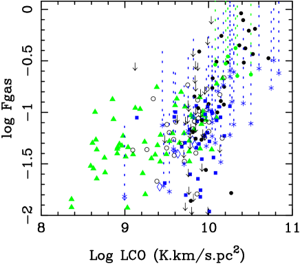
Figure 10: Gas fraction=MH₂/(M(H₂)+M_∗) versus CO luminosity, assuming the same CO-to-H₂  conversion factor $\alpha$ = 0.8 M_⊙ (K  km s^-1  pc²)^-1. The points of the high-z samples (blue asterisks and green dots), have been continued by a dotted line joining the two extreme values of gas fraction, obtained with $\alpha$=0.8 and 4.6. We indicate these lines only for the points in the high-z samples for which the MW conversion factor was selected by the authors. All symbols are as defined in Fig 6.

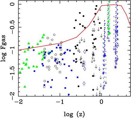
Figure 11: The gas fraction as in Figure 10, but versus redshift z. The red curve is a schematic line summarizing the evolution of cosmic star formation density, from the compilation by Hopkins & Beacom (2006), complemented with the GRB data by Kistler et al. (2009) and the optical data from Bouwens et al. (2008). The red curve is logarithmic and only indicative of relative variations of the SFR per cubic Mpc as a function of redshift, and can be translated vertically.

4.7 Activity of the galaxies

To determine what is triggering and regulating the starburst activity in our sample galaxies, it is interesting to try to determine which galaxies are morphologically perturbed or interacting, and to infer the activity status of their nucleus. The last column of Table 3 indicates the classification of nuclear AGN activity and/or possible minor or major interactions. The latter have been derived from the available images, either from HST, or presented by Stanford et al. (2000), or SDSS images. Some of the HST images of galaxies detected in CO are shown in Figure 12, the rest in the Appendix. The strong or weak interactions were determined from the relative fraction of the light in the tidal tails or perturbed features. No interaction means that the galaxy image looks unperturbed.

At high infrared luminosities, the fraction of Seyfert is about 50% in local ULIRGs, and their fraction increases steeply with L_FIR (Veilleux et al. 1999). The tight link between CO and infrared luminosities, however, shows that the dust heating is dominated by the starburtst in these objects (Iono et al. 2009). Among our 39 objects, 13 are known as AGN, and seven of these are detected in CO, implying a detection rate of more than 50%, higher than that of the whole sample. The percentage of weak and strong interactions in the whole sample are 23% and 28%, respectively, while in the detected object sample they are both 33%. There is thus a slight correlation between CO detection and interactions, however not at high significance. For more stringent conclusions, higher spatial resolution images need to be obtained for the half of the sample without HST data.

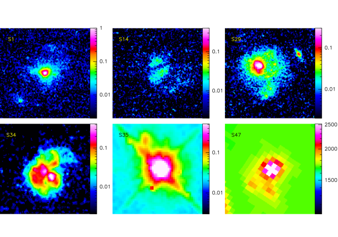
Figure 12: Optical or NIR images from HST. Most images are ACS-F814W, except S35 (WFPC2-702W) and S47 (WFC3-160W). All sources are detected in CO. Each panel is 5^′′x5^′′ in size, and is centered on the galaxy coordinates given in Table 1. The brightness scale is logarithmic (except for S47). North is up and east to the left in all panels. S14, S29, S34 and S47 were classified as strongly interacting, while S1 and S35 are weakly interacting.

4.8 Star formation efficiency

As in Paper II, we define the star formation efficiency as SFE = L_FIR/M(H₂), assuming a constant CO-to-H₂  conversion factor. The average SFE in our 0.6 $<$ z $<$ 1 sample is 595 L_⊙/M_⊙, comparable to that of the 0.2$<$z$<$0.6 sample. We plot SFE versus L_FIR in Figure 13, and versus redshift in Figure 14.

Our intermediate-z sample shows some of the highest efficiencies in star formation. The most extreme objects, with SFE $>$ 1000 L_⊙/M_⊙  are mostly interacting or perturbed, such as S1, S2, S4, S5, S11, S14, S20 and S25. While there is a relatively good correlation between SFE and L_FIR, it is not the case for L’_CO. The last shows only two populations of objects, with the local starbursts at low efficiency and gas content, separated from the higher-z samples. The SFE correlates much better with the dust temperature. This was also found in Paper II, so we do not reproduce the figure here.

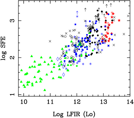
Figure 13: Star formation efficiency SFE=L_FIR/M(H₂), versus far-infrared luminosity L_FIR, assuming a single CO-to-H₂  conversion factor of $\alpha$ = 0.8 M_⊙ (K  km s^-1  pc²)^-1. All symbols are as defined in Fig 6.

Finally, the evolution of SFE with redshift is shown in Figure 14. There is an obvious rise of the envelope between z=0.2 and 1, precisely in the range of our sample. The amplitude of the rise appears, however, lower than that of the cosmic star formation history, as compiled by Hopkins & Beacom (2006). Figure 11 shows that the redshift variations of the gas fraction have a larger amplitude. The star formation evolution is certainly due to a combination of factors, essentially the gas fraction and the efficiency. Both vary with redshift in a similar manner, and it cannot be concluded which is the most determinant parameter

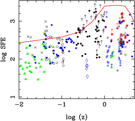
Figure 14: Same as Figure 13, but versus redshift. The red line is the same as in Figure 11. The SFE shows comparable evolution with z as the gas fraction shows.

To search for a possible correlation between the SFE and the compactness of the starburst, we computed the half-light radii of galaxies in our sample, using the GALFIT software version 3.0.4 (Peng et al. 2002, 2010). Red images in the I-band were used at intermediate z, with the highest possible angular resolution: HST images when available, and SDSS images for the remaining galaxies. A single-component Sersic model was fit to all images, giving an effective radius, which is displayed in Table 3. With respect to compactness, it is interesting to compare our sample with local star-forming galaxies. For that, we obtained the effective radii in the B-band for some local galaxies, from HyperLeda (Paturel et al. 2003). This band is the best at z=0 to correspond with the I-band at intermediate redshift. The SFE is plotted versus the half-light radii of galaxies R_1/2, when available, in Figure 15. There is only a slight trend for SFE to be anticorrelated to R_1/2, or correlated to the compactness of the blue light distribution, which reflects the star formation. The compactness of the starburst might be better traced by the molecular gas distribution, but this requires high resolution mapping of the high-z galaxies.

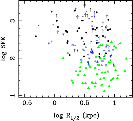
Figure 15: Same as Figure 13, but versus half-light radius.

5 Discussion and conclusions

We have presented the completion of our survey of the gas content in galaxies at intermediate redshift, through CO observations in a sample of 39 ULIRGs with redshifts between 0.6 and 1.0. Together with our earlier work (Paper II), this eliminates the CO desert in this highly relevant epoch (0.2$<$z$<$1), in which the SFR in the universe decreased by a factor 10. The CO detection rate between z=0.6 and 1 is 38%, significantly lower than between z=0.2 and 0.6 (60%, cf Paper II). The CO luminosity and, therefore, the derived H₂  mass are increasing with redshift by about a factor 4 up to z=1. We estimated the stellar mass of all sample objects through SED fitting of the optical and near-infrared fluxes and derived gas fractions. The evolution of the gas fraction with redshift is very pronounced, with a behavior reminiscent of the SFR evolution, suggesting that the gas fraction plays a large role in determining the star formation history.

We also checked the evolution of star formation efficiency with redshift, and found a trend comparable to that of the gas fraction. We concluded that both parameters play a significant role in setting the SFH. This can be seen in the envelope traced by the most extreme objects, but also in the averages over all detected objects, with or without taking the upper limits into account (Figure 16). To quantify this important point better, we averaged all SFE values and gas-to-stellar mass ratios over the redshift ranges z$<$0.2, and 0.2$<$ z $<$ 1.0, and computed the ratio between the two averaged values. The latter depend on whether the averages include the upper limits. The SFE at intermediate redshifts experiences a jump by a factor 2.1 (with detections only) and 3.8 (taking upper limits into account), while the ratio of M_gas/M_∗ rises by a factor 3.2 (with detections only) and 2.5 (taking upper limits into account). Given all these values, we can conclude that both SFE and the gas-to-stellar mass ratio were higher by a factor $3\pm 1$ at 0.2$<$z$<$1.0.

We checked whether the SFE is related to the compactness of the starburst, but found only a slight trend by SFE to decrease with half-light radius (Figure 15).

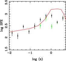
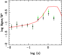
Figure 16: Evolution with redshift of averaged quantities, SFE to the left, and gas-to-stellar mass ratio to the right. The average of only detected points is plotted in green, and with the 3$\sigma$ upper limits in black (for high-z samples only). The error bars are the statistical ones following the square root of the number of points averaged. The red line is the same as in Figures 11 and 14.

Since the gas fraction depends on the CO-to-H₂ conversion ratio adopted, we observed a number of galaxies in both the CO(2-1) and CO(4-3) transitions to derive the gas excitation. The latter varies from source to source, but we find that in the majority the gas is significantly excited up to J=4, suggesting a high H₂  volume density and/or temperature. The comparison between the CO-derived gas mass and the dust mass derived from the far infrared fluxes supports the choice of the ULIRG conversion factor for our sources. This does not exclude some of the sources having low excitation, and their total gas mass has been underestimated. Spatial information on the CO emission is needed to better constrain this issue, and we will report the results of PdB interferometer imaging in a subsequent paper.

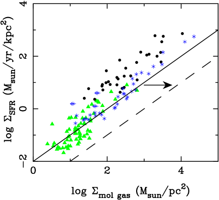
Figure 17: The Kennicutt-Schmidt relation between the gas surface density and the SFR surface density for the galaxies of our sample (filled black dots), compared to the galaxies from Gao & Solomon (2004, filled green triangles), and from Genzel et al (2010, blue asterisks). The full line corresponds to a depletion time of 100 Myr, and the dash line to 1 Gyr. A common conversion factor of $\alpha$ = 0.8 has been adopted here. The arrow indicates the direction and extent that all points will move, were an MW conversion factor to be used.

One caveat could be the bias introduced by selecting ULIRGs in our sample. It is true that our galaxies occupy the upper envelope of the SFR diagrams, either as a function of stellar mass, as in Fig. 9, or as a function of molecular gas, as in Fig. 17. There is, however, a continuity in the various categories, and the depletion time scales are progressive and overlapping, especially if the uncertainty on the CO-to-H₂  conversion factor is taken into account. This factor could vary smoothly across the observed galaxies, according to the kinetic temperature of the gas, its volume density, and its velocity dispersion. All these quantities could depend on the SFR, but also on its distribution and compactness (e.g. Shetty et al. 2011, Narayanan & Hopkins 2012, Feldmann et al. 2012).

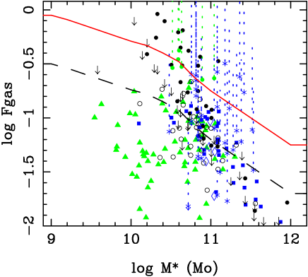
Figure 18: The gas fraction as in Figure 10, but versus stellar mass. The red line represents the predictions of cosmological simulations at z=1, and the black dashed line at z=0 from Davé et al. (2011).

Several physical parameters may intervene to account for the evolution of galaxies since z=1. First the gas fraction is a key parameter, and we have shown that indeed, its evolution in this redshift range is significant. The fueling of galaxies could be quenched by environmental effects, such as gas stripping and strangulation of star formation, through group and cluster formation during these epochs (e.g. Kimm et al. 2009). Also quenching could be morphological, due to the growth of spheroids (Martig et al. 2009). In addition to supernovae, or galactic winds, local photoionization of stars could regulate star formation above a critical SFR, which depends on mass and redshift, such as to explain the decline of cosmic SFR between z=1 and 0 (Cantalupo 2010). Second is the star formation efficiency, which could be higher, because triggered either by galaxy interactions and mergers, which have been more frequent in the past, but also through cold gas accretion, which is also thought to be efficient at these epochs (Keres et al. 2005). The last mechanism can also produce high gas fraction, resulting in instability-driven turbulence, perturbed disks, and clumpy gas distributions. This could mimick galaxy interactions in the observable morphology. Between z=1 and 0, hydrodynamical and semi-analytic studies predict a quenching of star formation, beginning at high stellar mass, and progressively involving lower masses (e.g. Gabor et al. 2010, Davé et al. 2011). It is interesting to compare observations of the gas fraction versus mass, to better constrain the models, since they have not yet reached coherence with observations. Figure 18 displays this relation, with the model lines superposed for z=0 and 1. They represent the best-fit models, corresponding to the no-wind simulation from Davé et al. (2011). Even if winds are neglected, the gas fraction slowly decreases with time because the intergalactic gas accretion rate decreases faster than the gas consumption rate in star formation. The consideration of stellar winds and, in particular, the momentum-driven winds are necessary to reproduce metallicity evolution, but all wind models lead to an under prediction of the gas fraction in small galaxies. Other quenching mechanisms are also necessary for massive galaxies, such as the influence of AGN feedback (Di Matteo et al. 2005).

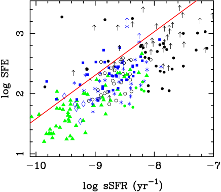
Figure 19: The star formation efficiency SFE (which varies as the inverse of the depletion time scale for the molecular gas) versus the specific star formation rate sSFR, in yr^-1. The red line is the fit from the COLD GASS sample of star-forming galaxies at z=0, from Saintonge et al. (2011b).

Another interesting parameter is the specific SFR, or SFR normalized by the stellar mass, which gives the time scale of formation of all the stellar mass in a galaxy at the given present SFR. We observe a good correlation with the star formation efficiency, in Figure 19. We note, however, that the quantities on the vertical and horizontal axes are not independent, since they both contain SFR. This correlation has been studied, in particular, by Saintonge et al. (2011b), who interpret the SFE as the depletion time scale for the molecular gas. With respect to our definition of SFE, the depletion time scale t_dep in yr is such that log(t_dep) = 9.76 -log(SFE). The diagram helps to clearly identify the main sequence of star formation, where galaxies have a continuous SFR, and the depletion time scale should be comparable to the stellar-mass forming time scale. We have superposed the best fit line for the sample COLD GASS of 222 normal star-forming galaxies at z=0. Our galaxies are generally below the line, because of their larger gas content.

The observations discussed in this work cover most of the age of the universe (out to $z=1$) and virtually all of the increase in the cosmic SFR. Both an increase in gas-to-stellar mass ratio and an increase in the SFE are responsible for the high cosmic SFR observed at earlier epochs. Depending on whether upper limits are taken into account, the M_gas/M_∗ ratio increases by a factor 3.2 (with detections only) and 2.5 (taking upper limits into account) and the SFE rises by factors of 2.1 and 3.8, respectively. The two factors are therefore equally significant, and only the combination of the two can explain the large increase in star formation between z=0 and 1.

Appendix A Available images for more sources

We present in this Appendix the remaining HST images of the sources, which give insight into their morphology.

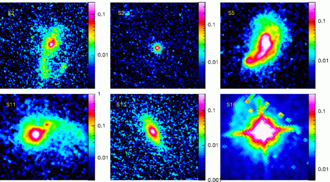
Figure 20: Optical red (F814W) HST-ACS images of six more sources. Only S16 is detected in the CO line. Each panel is 5^′′x5^′′ in size, and is centered on the galaxy coordinates of Table 1. The brightness scale is logarithmic. North is up and east to the left in all panels.

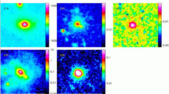
Figure 21: Same as in Fig 20, except for S18, which is a NICMOS-F160W image. S22 and S30 are detected in CO.