Universal non-adiabatic holonomic gates in quantum dots and single-molecule magnets

Abstract

Geometric manipulation of a quantum system offers a method for fast, universal, and robust quantum information processing. Here, we propose a scheme for universal all-geometric quantum computation using non-adiabatic quantum holonomies. We propose three different realizations of the scheme based on an unconventional use of quantum dot and single-molecule magnet devices, which offer promising scalability and robust efficiency.

1 Introduction

Holonomic quantum computation (HQC), originally conceived by Zanardi and Rasetti [1], has become one of the key approaches to perform robust quantum computation. The idea of HQC is based on the Wilczek-Zee holonomy [2] that generalizes the Berry phase [3] to non-Abelian (non-commuting) geometric phases accompanying adiabatic evolution. It was shown in Ref. [1] that adiabatic quantum holonomies generically allow for universal quantum computation. Different physical settings for adiabatic HQC have been proposed [4, 5, 6].

Recently, universal HQC based on Anandan’s non-adiabatic non-Abelian geometric phase [7] has been proposed [8]. This scheme allows for high-speed implementations of quantum gates; a feature that can be particularly useful in solid-state devices, where qubits typically have short coherence time. Non-adiabatic HQC can be made robust to a wide class of errors, such as decay, dephasing, and fluctuations in control parameters [9], and can be realized in decoherence free subspaces and noiseless subsystems insensitive to various collective errors [10, 11]. First experimental demonstrations of the scheme for universal non-adiabatic HQC proposed in Ref. [8] have been carried out for a superconducting qubit [12] and in an NMR system [13].

Here, we develop a setting for conditional holonomic gates in a four-level configuration. We illustrate how non-adiabatic holonomic gates in our scheme can be implemented in solid state devices consisting of few-electron quantum dots [14] and single-molecule magnets (SSMs) [15], which are promising candidates for quantum computation [16, 17, 18, 19]. By utilizing the scalability of these systems, the geometric nature of the proposed holonomic gates is a feature that may allow for robust and fast manipulations of a large number of qubits.

The outline of the paper is as follows. In the next section, we demonstrate one- and two-qubit quantum gates based on non-adiabatic quantum holonomies. The scheme is based on a generic four-level model with off-diagonal $2\times 2$ couplings. Realizations of the model in various kinds of solid-state devices are identified and examined in Sec. 3. The paper ends with the conclusions.

2 Non-adiabatic quantum holonomy

The general structure of our system is described by a four-dimensional effective state space whose dynamics is governed by a Hamiltonian of the form

$$H(t)=\hbar\Omega(t)\left(\begin{array}[]{rr}0&T\\ T^{\dagger}&0\end{array}\right),$$ (3)

in the ordered orthonormal basis $\mathcal{M}=\{|a\rangle,|b\rangle,|c\rangle,|d\rangle\}$. We assume that $T$ is a complex-valued and time-independent $2\times 2$ matrix that satisfies $\det T\neq 0$, where the latter ensures that $T$ is invertible. The Hamiltonian is turned on and off as described by the time-dependent scaling function $\Omega(t)$. We demonstrate in the following how $H(t)$ can be used for universal non-adiabatic HQC and how it can be realized in systems of four coupled quantum dots or in triangular molecular antiferromagnets.

The Hamiltonian in Eq. (3) naturally splits the state space into two subspaces spanned by $\mathcal{M}_{0}=\{|a\rangle,|b\rangle\}$ and $\mathcal{M}_{1}=\{|c\rangle,|d\rangle\}$. Non-adiabatic holonomy transformations are realized if (i) the Hamiltonian vanishes on each evolving subspace, and (ii) the projection operators $P_{0}=|a\rangle\langle a|+|b\rangle\langle b|$ and $P_{1}=|c\rangle\langle c|+|d\rangle\langle d|$ move in a cyclic fashion. Condition (i) is satisfied since $P_{l}(t)H(t)P_{l}(t)=U(t,0)P_{l}H(t)P_{l}U^{\dagger}(t,0)=0$, $l=0,1$, where the first equality follows from the fact that $H(t)$ commutes with the time evolution operator $U(t,0)=e^{-(i/\hbar)\int_{0}^{t}H(s)ds}$. For condition (ii), we first note that since $T$ is assumed to be invertible, there is a unique singular value decomposition $T=U_{0}DU_{1}^{\dagger}$, where $D={\textrm{diag}}\{\alpha,\beta\}$ and $U_{0},U_{1}$ are the positive and unitary parts, respectively. By using the singular value decomposition, the time evolution operator can be expressed as

$$U(t,0) = \left(\begin{array}[]{cc}U_{0}\cos\left(a_{t}D\right)U_{0}^{\dagger}&-iU_{0}\sin\left(a_{t}D\right)U_{1}^{\dagger}\\ -iU_{1}\sin\left(a_{t}D\right)U_{0}^{\dagger}&U_{1}\cos\left(a_{t}D\right)U_{1}^{\dagger}\end{array}\right)\hskip 14.22636pt$$ (6)

where $a_{t}=\int_{0}^{t}\Omega(s)ds$. The evolution of the $P_{l}$’s is thus cyclic provided there is a $t=\tau$ such that $\sin\left(a_{\tau}D\right)={\textrm{diag}}\{\sin(a_{\tau}\alpha),\sin(a_{\tau}\beta)\}=0$. Under this condition the holonomy matrices for the two subspaces $l=0,1$ read

$$U(\mathcal{C}_{l}) = U_{l}Z^{n}U_{l}^{\dagger},\ n=0,1,$$ (7)

where $\cos\left(a_{\tau}D\right)=Z^{n}$ with $Z={\textrm{diag}}\{1,-1\}$. $\mathcal{C}_{0}$ and $\mathcal{C}_{1}$ are the paths of the two subspaces spanned by $\mathcal{M}_{0}$ and $\mathcal{M}_{1}$, respectively. These paths reside in the Grassmannian manifold $G(4;2)$, being the space of all two-dimensional subspaces of the four-dimensional state space. One can see from Eq. (7) that the holonomy is non-trivial if and only if $n=1$.

Next, we encode the basis states in $\mathcal{M}$ into the computational two-qubit states $|a\rangle\rightarrow|00\rangle$, $|b\rangle\rightarrow|01\rangle$, $|c\rangle\rightarrow|10\rangle$, and $|d\rangle\rightarrow|11\rangle$. Running the Hamiltonian $H(t)$ along certain time intervals for appropriate choices of $T$ provides a realization of holonomic conditional gates of the form

$$U(\mathcal{C}_{0},\mathcal{C}_{1})=|0\rangle\langle 0|\otimes U(\mathcal{C}_{0})+|1\rangle\langle 1|\otimes U(\mathcal{C}_{1}),$$ (8)

where the holonomies $U(\mathcal{C}_{0})$ and $U(\mathcal{C}_{1})$ act on the target qubit conditionalized on the states $|0\rangle$ and $|1\rangle$, respectively, of the control qubit. One can see that by switching the roles of control and target qubits, which can be done by swapping the encoding of states $|b\rangle$ and $|c\rangle$, holonomic conditional two-qubit gate of the form $U(\mathcal{C}_{0})\otimes|0\rangle\langle 0|+U(\mathcal{C}_{1})\otimes|1\rangle\langle 1|$ can be carried out.

We now verify that $U(\mathcal{C}_{0},\mathcal{C}_{1})$ is sufficient for implementing a universal set of one- and two-qubit gates. The key observation is that any triplet $U_{0},U_{1},$ and $D$ can be realized since $T$ is arbitrary up to the condition $\det T\neq 0$. First, by choosing $T>0$ such that $\cos\left(a_{\tau}D\right)=Z$, it follows that $U_{1}=U_{0}$ and $U(\mathcal{C}_{0},\mathcal{C}_{1})$ reduces to the one-qubit holonomic gate $U_{0}ZU_{0}^{\dagger}={\bf n}\cdot{\bf R}$ with ${\bf R}=(X,Y,Z)$ the Pauli operators acting on the target qubit and ${\bf n}$ a unit vector. Any given ${\bf n}$, characterized by the spherical polar angles $\theta,\phi$, can for instance be realized by choosing $T=U_{0}DU_{0}^{\dagger}$ and $a_{\tau}$, such that $a_{\tau}D=\pi{\textrm{diag}}\{2,1\}$ and $U_{0}=e^{-i\phi Z/2}e^{-i\theta Y/2}$. By applying sequentially two such gates with different $T$’s corresponding to ${\bf n}$ and ${\bf m}$ yields $({\bf m}\cdot{\bf R})({\bf n}\cdot{\bf R})={\bf n}\cdot{\bf m}-i({\bf n}\times{\bf m})\cdot{\bf R}$, which is an arbitrary SU(2) transformation acting on the target qubit. Thus, our setup allows for arbitrary holonomic one-qubit gates. Secondly, by choosing $T$ with $U_{1}\neq U_{0}$ and $\cos\left(a_{\tau}D\right)=Z$ implements the holonomic conditional gate $U(\mathcal{C}_{0},\mathcal{C}_{1})=|0\rangle\langle 0|\otimes U_{0}ZU_{0}^{\dagger}+|1\rangle\langle 1|\otimes U_{1}ZU_{1}^{\dagger}$ that may entangle the qubits. Any entangling two-qubit gate is universal when assisted by arbitrary single-qubit transformations [20]. In other words, our scheme is universal.

Conceptually, the proposed holonomic conditional gate $U(\mathcal{C}_{0},\mathcal{C}_{1})$ can be viewed as a non-Abelian version of the Abelian geometric phase shift gate developed in Ref. [21, 22, 23]. In the Abelian case, evolution is chosen such that two orthogonal qubit states $|0\rangle$ and $|1\rangle$, say, pick up zero dynamical phases (for instance, by parallel transporting $|0\rangle$ and $|1\rangle$), which implies that $|0\rangle\rightarrow e^{i\gamma_{g}}|0\rangle$ and $|1\rangle\rightarrow e^{-i\gamma_{g}}|1\rangle$, $\gamma_{g}=\frac{1}{2}\Omega$ being the Aharonov-Anandan (AA) geometric phase [24] with $\Omega$ the solid angle enclosed on the Bloch sphere. This defines the AA geometric phase gate $|k\rangle\rightarrow e^{i(1-2k)\gamma_{g}}|k\rangle$, $k=0,1$. In our non-Abelian scheme, conditional two-qubit gate is implemented if there exist pair of loops $\mathcal{C}_{0}$ and $\mathcal{C}_{1}$ in the Grassmannian manifold $G(4;2)$ of the target qubit along which there is no dynamical phase. Note that the orthogonal subspaces $\mathcal{M}_{0}$ and $\mathcal{M}_{1}$ correspond to the state space of the target qubit when the control qubit is in the state $|0\rangle$ or $|1\rangle$, respectively. Zero dynamical contribution to the evolution of these two orthonormal subspaces is a signature of the geometric nature of our holonomic conditional two-qubit gate, just as zero dynamical phase in the Abelian schemes [21, 22, 23] is a signature of the geometric nature of the above AA gates.

3 Physical implementations

3.1 Coupled quantum dots

3.1.1 Tight-binding model

As possible physical implementations of the holonomic gates, we here discuss two settings involving four coupled quantum dots arranged in closed ring geometry. The first setting involves the well-known two-dimensional electron gas supported, e.g., by a GaAs/AlGaAs heterostructure, depleted by a convenient set of top gate electrodes to form four quantum dots where electrons are confined. Devices of this type can be routinely fabricated nowadays with state of the art electron beam lithography [25]. In this system, electrons can tunnel from one dot to another with a tunnel coupling controlled individually by inter-dot gates. We also assume that the local potential, and hence the available single-particle energy levels in each quantum dot, can be individually manipulated with back gates. HQC is realized when this four-quantum-dot device contains just a single electron. If only one single-particle orbital in each quantum dot is relevant, the system can be described by a four-site tight-binding model, forming a closed ring. The second-quantized Hamiltonian reads

$$H=\sum_{k=1,\sigma}^{4}\epsilon_{k}c_{k,\sigma}^{\dagger}c_{k,\sigma}^{\phantom{\dagger}}+\sum_{k=1}^{4}\left[t_{k,k+1}c_{k,\sigma}^{\dagger}c_{k+1,\sigma}^{\phantom{\dagger}}+h.c.\right],\ \$$ (9)

where $c_{k\sigma}^{\dagger}$ ($c_{k\sigma}^{\phantom{\dagger}}$) are electron creation (annihilation) operators for Wannier orbitals localized at dot-site $k$, with on-site energy $\epsilon_{k}$ and spin quantum number $\sigma=\uparrow,\downarrow$; we assume periodic boundary conditions $c_{5,\sigma}=c_{1,\sigma}$. The $t_{k,k+1}$ are nearest-neighbor hopping parameters, which can be controlled by gate voltages.

In the presence of an external magnetic field $B$, the Hamiltonian in Eq. (9) acquires the Zeeman term $-gB\sum_{k\sigma}\sigma c_{k\sigma}^{\dagger}c_{k\sigma}^{\phantom{\dagger}}$, where the Bohr magneton has been absorbed into $g$. Furthermore, the magnetic field generates a gauge-invariant modification of the tight-binding hopping parameters via the Peierls phase factors [26, 27, 28]

$$t_{k,k+1}\rightarrow J_{k,k+1}=t_{k,k+1}e^{-i\frac{e}{\hbar}{\alpha_{k,k+1}}}\;,$$ (10)

where $\alpha_{k,k+1}=\int_{k\rightarrow k+1}\mathbf{A}\cdot d\mathbf{l}$ is the integral of the vector potential along the hopping path from site $k$ to site $k+1$.

We fix the on-site energies $\epsilon_{k}=0$ by adjusting the voltage on the back gates of the device. We now assume that hopping parameters can be turned on and off with the same time-dependent scaling function $\Omega(t)$ by sweeping the top gates. In the invariant Fock subspace spanned by the four (spin-polarized) one-electron states $\{|\uparrow\!000\rangle,|00\!\uparrow\!0\rangle,|0\!\uparrow\!00\rangle,|000\!\uparrow\rangle\}$, the time dependent Hamiltonian in this ordered basis has the form of Eq. (3), with the time-independent $2\times 2$ submatrix

$$T=\left(\begin{array}[]{cc}\mathcal{J}_{1,2}&\mathcal{J}_{4,1}^{\ast}\\ \mathcal{J}_{2,3}^{\ast}&\mathcal{J}_{3,4}\\ \end{array}\right),$$ (13)

where we have put $J_{k,k+1}=\hbar\Omega(t)\mathcal{J}_{k,k+1}$. Note that for a given magnetic field we must choose the complex-valued hopping parameters so that their phases $\alpha_{k,k+1}$ add up to the total magnetic flux $\Phi=\oint\mathbf{A}\cdot d\mathbf{l}={\cal A}B$, where $\cal A$ is the area enclosed by the four-dot ring. A change of these phases corresponds to a gauge transformation $\mathbf{A}\rightarrow\mathbf{A}+\nabla\Lambda$ under which the holonomies of the two subspaces $l=0,1$ transform into $U(\mathcal{C}_{l})\rightarrow\Gamma_{l}U(\mathcal{C}_{l})\Gamma_{l}^{\dagger}$, where $\Gamma_{l}={\textrm{diag}}\{e^{-i\frac{e}{\hbar}\Lambda(l+1)},e^{-i\frac{e}{\hbar}\Lambda(l+3)}\}$ with $\Lambda(k)$ indicating the value of $\Lambda$ at site $k$. This shows the holonomies associated with this field-dependent tight-binding Hamiltonian are gauge covariant quantities.

In order to take advantage of non-adiabaticity to control decoherence effects, the typical switching time $\tau$ should be as short as possible. At the same time, the action of the Hamiltonian must be ”adiabatic” enough to prevent transitions to higher orbital levels not included in Eq. (9). This requirement is expressed by the condition $\tau\gg\hbar/\Delta\epsilon$, where $\Delta\epsilon$ is the single-particle level spacing. For a quantum dot with a size of 100 nm, typically $\Delta\epsilon\sim 1{\rm meV}$, which would permit $\tau$ to be as fast as 10 ps. This time is considerably shorter than the phase coherence time for charge qubits in quantum dots ($\sim$ 1-10 ns [25]).

3.1.2 Spin model

As the second setting to realize our scheme, we start again with the four-dot system introduced above, but we consider the case where four electrons are confined in the device. Now, electron-electron interactions must be included and we can do so by adding to the Hamiltonian of Eq. (9) an onsite Hubbard repulsion term $U\sum_{k}n_{k\uparrow}n_{k\downarrow}$, where $n_{k\sigma}=c_{k\sigma}^{\dagger}c_{k\sigma}^{\phantom{\dagger}}$. In the limit $t_{k,k+1}/U\ll 1$ double occupancy in each dot is suppressed and the low-energy physics of the system can be described by the spin Hamiltonian [29]

$$\tilde{H}_{\textrm{s}} = \sum_{k=1}^{4}\tilde{J}_{k,k+1}{\bf s}_{k}\cdot{\bf s}_{k+1}+\sum_{k=1}^{4}{\bf s}_{k}\cdot\Theta_{k,k+1}{\bf s}_{k+1}$$ (14)

$$+\sum_{k=1}^{4}\tilde{{\bf D}}_{k,k+1}\cdot\left({\bf s}_{k}\times{\bf s}_{k+1}\right),$$

where ${\bf s}_{k}$ is a spin$-\frac{1}{2}$ vector operator localized at site $k$. In Eq. (14), the first term is an isotropic Heisenberg interaction, with antiferromagnetic exchange coupling $\tilde{J}_{k,k+1}$, the second term is an anisotropic exchange described by second rank symmetric tensors $\Theta_{k,k+1}$, and the last term is an antisymmetric Dzialoshinski-Moriya (DM) interaction. The general exchange coupling arises from the interplay between the electron-electron repulsion and spin-orbit interaction. For the geometry of four coplanar quantum dots in the $xy$ plane only $z$ components of the DM exchange vectors $\tilde{{\bf D}}_{k,k+1}$ are relevant. In an in-plane electric field, the parameters in Eq. (14) can be modified so that the effective Hamiltonian of the spin-model is given by

$$H_{\textrm{s}}=\sum_{k=1}^{4}{\bf s}_{k}\cdot\bar{\bar{J}}_{k,k+1}{\bf s}_{k+1}+\sum_{k=1}^{4}D_{k,k+1}^{z}\cdot\left({\bf s}_{k}\times{\bf s}_{k+1}\right)_{z}.\hskip 14.22636pt$$ (15)

Here, we have $\bar{\bar{J}}_{k,k+1}=\textrm{diag}\{J_{k,k+1},J_{k,k+1},0\}$ with $J_{k,k+1}\sim t_{k,k+1}^{2}/U$ and ${D}^{z}_{k,k+1}\sim t_{k,k+1}\lambda_{k,k+1}/U$, where $\lambda_{k,k+1}$ is a spin-dependent hopping term describing the spin-orbit interaction.

Let $|\uparrow\rangle_{k}$ $(|\downarrow\rangle_{k})$ be the eigenvector of the $z$ component of the spin operator at site $k$ corresponding to the eigenvalue $\frac{1}{2}$ $(-\frac{1}{2})$. The four-dimensional subspace with $S_{\rm total}^{z}=1$, spanned by the ordered basis $\mathcal{M}=\{|\downarrow\uparrow\uparrow\uparrow\rangle,|\uparrow\uparrow\downarrow\uparrow\rangle,|\uparrow\downarrow\uparrow\uparrow\rangle,|\uparrow\uparrow\uparrow\downarrow\rangle\}$ is an invariant subspace [30]. To realize the HQC scheme, the parameters $J_{k,k+1}$ and $D_{k,k+1}^{z}$ have to be turned on and off with the same time-dependent function $\Omega(t)$. Under this condition, the Hamiltonian in the ordered basis $\mathcal{M}$ has exactly the form of Eq. (3) with the time-independent submatrix

$$T=\left(\begin{array}[]{cc}\mathcal{J}_{1,2}-i\mathcal{D}_{1,2}^{z}&\mathcal{J}_{4,1}+i\mathcal{D}_{4,1}^{z}\\ \mathcal{J}_{2,3}+i\mathcal{D}_{2,3}^{z}&\mathcal{J}_{3,4}-i\mathcal{D}_{3,4}^{z}\\ \end{array}\right),$$ (18)

where we have put $J_{k,k+1}=\hbar\Omega(t)\mathcal{J}_{k,k+1}$ and $D^{z}_{k,k+1}=\hbar\Omega(t)\mathcal{D}^{z}_{k,k+1}$. It is important to stress that since both $J_{k,k+1}$ and $D^{z}_{k,k+1}$ are proportional to the inter-dot tunneling constants, they can be efficiently manipulated with time-dependent gate voltages.

3.2 Single-molecule magnet

The spin Hamiltonian in Eq. (14) also describes the magnetic properties of a class of single-molecule magnets (SSMs) composed of antiferromagnetic spin rings [15]. Such systems would in principle be more scalable, compact, and reproducible than the devices based on quantum dots, since their exchange constants and spin coherence properties are controlled by the molecular structure of the molecule, which can be chemically engineered [31].

The systems that we are interested in are triangular SMMs such as $\textrm{Cu}_{3},\textrm{V}_{15},\textrm{Co}_{3}$ [32, 33]. Their magnetic core consists of three $s=1/2$ spins positioned at the vertexes of an equilateral triangle and coupled by an antiferromagnetic Heisenberg exchange interaction. The ground state (GS) manifold of these frustrated SMMs is given by two degenerate total spin $S=1/2$ doublets ($M=\pm 1/2$) of opposite spin chirality $\chi=\pm 1$. The energy gap $\Delta_{J}$ to the first excited $S=3/2$ quadruplet is typically in the order of 1 meV. A spin-orbit induced DM interaction lifts the degeneracy between the two chiral doublets with a splitting $\Delta_{\textrm{SO}}\leq 0.1\Delta_{J}$ [34, 35]. What makes these triangular SMMs interesting for quantum manipulation is that, due to the lack of inversion symmetry, an electric field in the $xy$-plane of the molecule couples the two GS doublets of opposite chirality [34, 29, 36]. In the four-dimensional GS manifold spanned by the states $|\chi=\pm 1,M=\pm 1/2\rangle$, the effective low-energy spin Hamiltonian in the presence of external electric $\bf E$ and magnetic $\bf B$ fields is [34]

$$H_{\textrm{eff}}=\Delta_{\textrm{SO}}C_{z}S_{z}+d\;\textbf{E}\cdot\textbf{C}_{\parallel}+\textbf{B}\cdot\bar{\bar{g}}\textbf{S},$$ (19)

where $\textbf{C}=(\{\textbf{C}_{\parallel}=C_{x},C_{y}\},C_{z})$ and $\textbf{S}=(S_{x},S_{y},S_{z})$ are respectively the chirality and spin operators. Due to the symmetry of the molecule $\bar{\bar{g}}=\textrm{diag}\{g_{\parallel},g_{\parallel},g_{\bot}\}$. The parameter $d$ is the effective electric dipole coupling, and it gives the strength of the coupling between the two states with opposite chirality brought about by the electric field. In Cu₃ SMMs $d$ is not small [36], and for typical electric fields generated by scanning tunneling microscope ($\approx 10^{2}$ kV/cm) the spin-chirality manipulation (Rabi) time is $10-10^{3}$ ps [34, 36].

To implement our holonomic scheme in this setting, we assume ${\bf B}$ and ${\bf E}$ are turned on and off by a common scaling function $\Omega(t)$ and that $B_{z}$ is negligibly small. Under these conditions, the Hamiltonian in Eq. (19) takes the form

$$H_{\textrm{eff}}=\hbar\Omega(t)\left(\begin{array}[]{cc}0&T\\ T^{\dagger}&0\\ \end{array}\right)+\frac{\Delta_{\textrm{SO}}}{2}\left(\begin{array}[]{cc}I&0\\ 0&-I\\ \end{array}\right)$$ (24)

in the ordered basis $\{|+1,+1/2\rangle$, $|-1,-1/2\rangle$, $|+1,-1/2\rangle$, $|-1,+1/2\rangle\}$ of the ground state subspace. Here, $T_{11}=T_{22}^{*}=\frac{1}{2}(\mathcal{B}_{x}-i\mathcal{B}_{y})$ and $T_{12}=T_{21}^{*}=(\mathcal{E}_{x}-i\mathcal{E}_{y})$, where we have put $g_{\parallel}B_{k}=\hbar\Omega(t)\mathcal{B}_{k}$ and $dE_{k}=\hbar\Omega(t)\mathcal{E}_{k}$, $k=x,y$. This expression of the Hamiltonian shows that triangular SMMs such as Cu₃ can be used to implement efficient and robust gates. Although the restricted form of $T$ associated with this system does not allow for universal computation, we would still be able to obtain some of the most important gates such as all the Pauli-matrices and the controlled-Z gate in a fashion that is highly resistant to errors. The crucial challenge relies on the ability of generating electric and magnetic fields characterized by time-dependence function $\Omega(t)$. Fig. 1 shows the fidelity $F$ of the Pauli-Y gate performed with a triangular SMM, as a function of the spin-orbit induced splitting $\Delta_{\textrm{SO}}$ and operation time $\tau$. Here, we have adopted the definition [37] $F=F(W,V)=\frac{1}{2}+\frac{1}{8}{\textrm{Re}}\Tr\left(W^{\dagger}V\right)$, where $W$ is the ideal gate and $V$ is the gate carried out by the perturbative Hamiltonian in Eq.  (24). The fidelity $F(W,V)$ determines the Hilbert-Schmidt distance between $W$ and $V$. For typical values of $\Delta_{\textrm{SO}}\approx 0.02$ meV [35] the fidelity is over $98\%$ for $\tau=10-100$ ps.

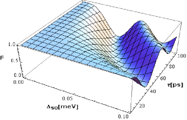
Figure 1: Fidelity $F$ of the holonomic Y-gate for a triangular SMM as a function of the spin-orbit induced splitting $\Delta_{\textrm{SO}}$ and operation time $\tau$. Here we have chosen $g_{\parallel}(B_{x}-iB_{y})=3\hbar\Omega(t)$, $d(E_{x}-iE_{y})=-\frac{i}{2}\hbar\Omega(t)$, where $\Omega(t)$ is a square pulse such that $\int_{0}^{\tau}\Omega(t)dt=\pi$.

It is worth mentioning that the spin model described by the Hamiltonian in Eq. (15) can be realized in other settings, such as magnetic impurities on the surface of topological insulators [38], cold atoms in a two-dimensional optical lattice [39], and nuclear spin qubits interacting via a semiconductor-heterojunction [40]. These systems may provide alternative platforms to implementing our holonomic gates.

3.3 Scalability

The four-level configuration presented above can be used in a scalable pattern necessary for universal quantum computation on any number of qubits. This can be achieved by implementing the Hamiltonian

$$\widetilde{H}(t) = \sum_{p<q}\hbar\Omega_{pq}(t)\left(\begin{array}[]{rr}0&T^{(pq)}\\ T^{(pq)\dagger}&0\end{array}\right),$$ (27)

where $p$ and $q$ label the qubits. Any gate acting on qubits $p$ and $q$ can be implemented by turning on and off $\Omega_{pq}(t)$ while the other terms are kept off. $\widetilde{H}(t)$ can be realized with the first two examples using the techniques introduced in Ref. [41] to design scalable architectures in quantum dot systems. This Hamiltonian would also be realized by arranging triangular SMMs on a surface in a way that each of them can be manipulated individually.

4 Conclusions

In conclusion, we have introduced a scheme to implement high-speed universal holonomic quantum gates that considerably differs from the other setups proposed for HQC. It allows for implementation of conditional gates using non-adiabatic quantum holonomies [7] acting on qubit pairs encoded in a four level structure. We make use of the two-qubit system as a unit cell for scalable all-geometric quantum computation. We propose three different realizations of our scheme based on an unconventional use of quantum dot and single-molecule magnet devices. We emphasize that the physical realizations of HQC presented here differ substantially from previous proposals of implementation of charge and spin qubits in quantum dots and single-molecule magnets. Finally, we would like to point out that the four level configuration proposed here is quite a general scheme that can be realized with other physical systems actively considered for quantum computer implementation [38, 39, 40].

References

- [1] Zanardi P and Rasetti M 1999 Holonomic quantum computation Phys. Lett. A 264 94
- [2] Wilczek F and Zee A 1984 Appearance of gauge structure in simple dynamical systems Phys. Rev. Lett. 52 2111
- [3] Berry M V 1984 Quantal phase factors accompanying adiabatic changes Proc. Roy. Soc. London Ser. A 392 45
- [4] Duan L M, Cirac J I and Zoller P 2001 Geometric manipulation of trapped ions for quantum computation Science 292 1695
- [5] Faoro L, Siewert J and Fazio R 2003 Non-Abelian holonomies, charge pumping, and quantum computation with Josephson junctions Phys. Rev. Lett. 90 028301
- [6] Solinas P, Zanardi P, Zanghì N and Rossi F 2003 Semiconductor-based geometrical quantum gates Phys. Rev. B 67 121307
- [7] Anandan J 1988 Non-adiabatic non-Abelian geometric phase Phys. Lett. A 133 171
- [8] Sjöqvist E, Tong D M, Andersson L M, Hessmo B and Singh K 2012 Non-adiabatic holonomic quantum computation New J. Phys. 14 103035
- [9] Johansson M, Sjöqvist E, Andersson L M, Ericsson M, Hessmo B, Singh K and Tong D M 2012 Robustness of nonadiabatic holonomic gates Phys. Rev. A 86 062322
- [10] Xu G F, Zhang J, Tong D M, Sjöqvist E and Kwek L C 2012 Nonadiabatic holonomic quantum computation in decoherence-free subspaces Phys. Rev. Lett. 109 170501
- [11] Zhang J, Kwek L C, Sjöqvist E, Tong D M and Zanardi P 2013 Quantum computation in noiseless subsystems with fast non-Abelian holonomies arXiv:1308.1919 [quant-ph]
- [12] Abdumalikov A A, Fink J M, Juliusson K, Pechal M, Berger S, Wallraff A and Filipp S 2013 Experimental realization of non-Abelian non-adiabatic geometric gates Nature 496 482
- [13] Feng G, Xu G and Long G 2013 Experimental realization of nonadiabatic holonomic quantum computation Phys. Rev. Lett. 110 190501
- [14] Kouwenhoven L P, Austing D G and Tarucha S 2001 Few-electron quantum dots Rep. Prog. Phys. 63 701
- [15] Gatteschi D, Sessoli R and Villain J 2006 Molecular Nanomagnets (Oxford University Press, Oxford)
- [16] Leuenberger M N and Loss D 2001 Quantum computing in molecular magnets Nature 410 789
- [17] Tejada J, Chudnovsky E M, del Barco E, Hernandez J M and Spiller T P 2001 Magnetic qubits as hardware for quantum computers Nanotechnology 12 181
- [18] Hanson R, Kouwenhoven L P, Petta J R, Tarucha S and Vandersypen L M K 2007 Spins in few-electron quantum dots Rev. Mod. Phys. 79 1217
- [19] Żac R A, Röthlisberger B, Chesi S and Loss D 2010 Quantum computing with electron spins in quantum dots Riv. Nuovo Cimento 033 345
- [20] Bremner M J, Dawson C M, Dodd J L, Gilchrist A, HarrowA W, Mortimer D, Nielsen M A and Osborne T J 2002 Practical scheme for quantum computation with any two-qubit entangling gate Phys. Rev. Lett. 89 247902
- [21] Wang X B and Keiji M 2001 Phys Rev. Lett. 87 097901
- [22] Zhu S-L and Wang Z D 2002 Implementation of universal quantum gates based on nonadiabatic geometric phases Phys. Rev. Lett. 89 097902
- [23] Zhu S-L and Wang Z D 2003 Universal quantum gates based on a pair of orthogonal cyclic states: application to NMR systems Phys. Rev. A 67 022319
- [24] Aharonov Y and Anandan J 1987 Phase change during a cyclic quantum evolution Phys. Rev. Lett. 58 1593
- [25] Petersson K D, Petta J R, Lu H and Gossard A C 2010 Quantum coherence in a one-electron semiconductor charge qubit Phys. Rev. Lett. 105 246804
- [26] Graf M and Vogl P 1995 Electromagnetic fields and dielectric response in empirical tight-binding theory Phys. Rev. B 51 4940
- [27] Ismail-Beigi S, Chang E K and Louie S G 2001 Coupling of nonlocal potentials to electromagnetic fields Phys. Rev. Lett. 87 087402
- [28] Cehovin A, Canali C M and MacDonald A H 2004 Orbital and spin contributions to the g tensors in metal nanoparticles Phys. Rev. B 69 045411
- [29] Trif M, Troiani F, Stepanenko D and Loss D 2010 Spin electric effects in molecular antiferromagnets Phys. Rev. B 82 045429
- [30] Note that this subspace involves the excited states with of the spin Hamiltonian.
- [31] Wedge C J, Timco G A, Spielberg E T, George R E, Tuna F, Rigby S, McInnes E J L, Winpenny R E P, Blundell S J and Ardavan A 2012 Chemical engineering of molecular qubits Phys. Rev. Lett. 108 107204
- [32] Kortz U, Al-Kassem N K, Savelieff M G, Al Kadi N A and Sadakane M 2001 Synthesis and characterization of copper-, zinc-, manganese-, and cobalt-substituted dimeric heteropolyanions, [(-XW9O33)2 M3 (H2O)3]n- (n = 12, X = As, Sb, M = Cu2+, Zn2+; n = 10, X = Se, Te, M = Cu2+) and [(-As W9 O33)2 WO (H2O) M2 (H2 O)2]10- (M = Zn2+, Mn2+, Co2+) Inorg. Chem. 40 4742
- [33] Choi K-Y, Matsuda Y H, Nojiri H, Kortz U, Hussain F, Stowe A C, Ramsey C and Dalal N S 2006 Observation of a Half step magnetization in the Cu3-type triangular spin ring Phys. Rev. Lett. 96 107202
- [34] Trif M, Troiani F, Stepanenko D and D. Loss D 2008 Spin-electric coupling in molecular magnets Phys. Rev. Lett. 101 217201
- [35] Nossa J F, Islam M F, Canali C M and Pederson M R 2012 First-principles studies of spin-orbit and Dzyaloshinskii-Moriya interactions in the Cu3 single-molecule magnet Phys. Rev. B 85 085427
- [36] Islam M F, Nossa J F, Canali C M and Pederson M R 2010 First-principles study of spin-electric coupling in a Cu3 single molecular magnet Phys. Rev. B 82 155446
- [37] Our fidelity is the linear function of the scalar cost function introduced in [Cabrera R, Shir O M, Wu R and Rabitz H 2011 Fidelity between unitary operators and the generation of robust gates against off-resonance perturbations J. Phys. A: Math. Theor. 44 095302].
- [38] Zhu J-J, Yao D-X, Zhang S-C and Chang K 2011 Electrically controllable surface magnetism on the surface of topological insulators Phys. Rev. Lett. 106 097201
- [39] Radić J, Di Ciolo A, Sun K and Galitski V 2012 Exotic quantum spin models in spin-orbit-coupled Mott insulators Phys. Rev. Lett. 109 085303
- [40] Mozyrsky D, Privman V and Glasser M L 2001 Indirect interaction of solid-state qubits via two-dimensional electron gas Phys. Rev. Lett. 86 5112
- [41] Trifunovic L, Dial O, Trif M, Wootton J R, Abebe R, Yacoby A and Loss D 2012 Long-distance spin-spin coupling via floating gates Phys. Rev. X 2 011006