I Introduction
Directed polymers in a quenched random potential have
been the subject of intense investigations during the past two
decades (see e.g. hh_zhang_95 ; burgers_74 ; hhf_85 ; numer1 ; numer2 ; kardar_87 τ 𝜏 \tau [ 0 , t ] 0 𝑡 [0,t] V [ ϕ ( τ ) , τ ] 𝑉 italic-ϕ 𝜏 𝜏 V[\phi(\tau),\tau]
H [ ϕ ( τ ) , V ] = ∫ 0 t 𝑑 τ { 1 2 [ ∂ τ ϕ ( τ ) ] 2 + V [ ϕ ( τ ) , τ ] } ; 𝐻 italic-ϕ 𝜏 𝑉 superscript subscript 0 𝑡 differential-d 𝜏 1 2 superscript delimited-[] subscript 𝜏 italic-ϕ 𝜏 2 𝑉 italic-ϕ 𝜏 𝜏 H[\phi(\tau),V]=\int_{0}^{t}d\tau\Bigl{\{}\frac{1}{2}\bigl{[}\partial_{\tau}\phi(\tau)\bigr{]}^{2}+V[\phi(\tau),\tau]\Bigr{\}}; (1)
where the disorder potential V [ ϕ , τ ] 𝑉 italic-ϕ 𝜏 V[\phi,\tau] V ( ϕ , τ ) ¯ = 0 ¯ 𝑉 italic-ϕ 𝜏 0 \overline{V(\phi,\tau)}=0 δ 𝛿 \delta
V ( ϕ , τ ) V ( ϕ ′ , τ ′ ) ¯ = u δ ( τ − τ ′ ) δ ( ϕ − ϕ ′ ) ¯ 𝑉 italic-ϕ 𝜏 𝑉 superscript italic-ϕ ′ superscript 𝜏 ′ 𝑢 𝛿 𝜏 superscript 𝜏 ′ 𝛿 italic-ϕ superscript italic-ϕ ′ {\overline{V(\phi,\tau)V(\phi^{\prime},\tau^{\prime})}}=u\delta(\tau-\tau^{\prime})\delta(\phi-\phi^{\prime}) (2)
Here the parameter u 𝑢 u KPZ
In what follows we consider the problem in which the polymer is fixed
at the origin, ϕ ( 0 ) = 0 italic-ϕ 0 0 \phi(0)=0 τ = t 𝜏 𝑡 \tau=t V 𝑉 V
Z = ∫ − ∞ + ∞ 𝑑 x Z ( x ) = exp { − β F } 𝑍 superscript subscript differential-d 𝑥 𝑍 𝑥 𝛽 𝐹 Z=\int_{-\infty}^{+\infty}dx\;Z(x)\;=\;\exp\{-\beta F\} (3)
where
Z ( x ) = ∫ ϕ ( 0 ) = 0 ϕ ( t ) = x 𝒟 ϕ ( τ ) e − β H [ ϕ ] 𝑍 𝑥 superscript subscript italic-ϕ 0 0 italic-ϕ 𝑡 𝑥 𝒟 italic-ϕ 𝜏 superscript e 𝛽 𝐻 delimited-[] italic-ϕ Z(x)=\int_{\phi(0)=0}^{\phi(t)=x}{\cal D}\phi(\tau)\;\mbox{\Large e}^{-\beta H[\phi]} (4)
is the partition function of the system with the fixed boundary conditions,
ϕ ( 0 ) = 0 italic-ϕ 0 0 \phi(0)=0 ϕ ( t ) = x italic-ϕ 𝑡 𝑥 \phi(t)=x F 𝐹 F f 0 t subscript 𝑓 0 𝑡 f_{0}t f 0 subscript 𝑓 0 f_{0} F 𝐹 F F ~ ~ 𝐹 \tilde{F} t 𝑡 t t 𝑡 t F ~ ∝ t 1 / 3 proportional-to ~ 𝐹 superscript 𝑡 1 3 \tilde{F}\propto t^{1/3} hhf_85 ; numer1 ; numer2 ; kardar_87
F = f 0 t + c t 1 / 3 f 𝐹 subscript 𝑓 0 𝑡 𝑐 superscript 𝑡 1 3 𝑓 F\;=\;f_{0}t\;+\;c\,t^{1/3}\;f (5)
where c 𝑐 c f 𝑓 f t → ∞ → 𝑡 t\to\infty P ( f ) 𝑃 𝑓 P(f) 3 5 f 0 t subscript 𝑓 0 𝑡 f_{0}t
Z = exp { − β f 0 t } Z ~ 𝑍 𝛽 subscript 𝑓 0 𝑡 ~ 𝑍 Z\;=\;\exp\{-\beta f_{0}t\}\,\tilde{Z} (6)
so that
Z ~ = exp { − λ f } ~ 𝑍 𝜆 𝑓 \tilde{Z}\;=\;\exp\{-\lambda f\} (7)
where
λ = β c t 1 / 3 𝜆 𝛽 𝑐 superscript 𝑡 1 3 \lambda\;=\;\beta\,c\,t^{1/3} (8)
For the similar problem with the zero boundary conditions, ϕ ( 0 ) = ϕ ( t ) = 0 italic-ϕ 0 italic-ϕ 𝑡 0 \phi(0)=\phi(t)=0 KPZ-TW1 ; KPZ-TW2 ; BA-replicas ; LeDoussal1 BA-replicas ; LeDoussal1 Prolhac-Spohn 1 4 LeDoussal2 P ( f ) 𝑃 𝑓 P(f) LeDoussal2
Let us introduce the function
W ( f ) ≡ ∫ f ∞ 𝑑 f ′ P ( f ′ ) 𝑊 𝑓 superscript subscript 𝑓 differential-d superscript 𝑓 ′ 𝑃 superscript 𝑓 ′ W(f)\;\equiv\;\int_{f}^{\infty}\;df^{\prime}\;P(f^{\prime}) (9)
which gives the probability that the random free energy
is bigger that a given value f 𝑓 f t → ∞ → 𝑡 t\to\infty
W ( f ) = det ( 1 − K ^ − f ) ≡ F 1 ( − f ) 𝑊 𝑓 1 subscript ^ 𝐾 𝑓 subscript 𝐹 1 𝑓 W(f)\;=\;\det(1-\hat{K}_{-f})\;\equiv\;F_{1}(-f) (10)
with the kernel
K − f ( ω , ω ′ ) = Ai ( ω + ω ′ − f ) ; ( ω , ω ′ > 0 ) subscript 𝐾 𝑓 𝜔 superscript 𝜔 ′ Ai 𝜔 superscript 𝜔 ′ 𝑓 𝜔 superscript 𝜔 ′
0
K_{-f}(\omega,\omega^{\prime})\;=\;\operatorname{Ai}(\omega+\omega^{\prime}-f)\;;\;\;\;\;\;\;\;\;\;(\omega,\omega^{\prime}\;>0) (11)
which is the GOE Tracy-Widom distribution TW2 ; Ferrari-Spohn
F 1 ( s ) = exp [ − 1 2 ∫ s + ∞ 𝑑 ξ ( ξ − s ) q 2 ( ξ ) − 1 2 ∫ s + ∞ 𝑑 ξ q ( ξ ) ] subscript 𝐹 1 𝑠 1 2 superscript subscript 𝑠 differential-d 𝜉 𝜉 𝑠 superscript 𝑞 2 𝜉 1 2 superscript subscript 𝑠 differential-d 𝜉 𝑞 𝜉 F_{1}(s)\;=\;\exp\Biggl{[}-\frac{1}{2}\int_{s}^{+\infty}d\xi\;(\xi-s)\;q^{2}(\xi)\;-\frac{1}{2}\int_{s}^{+\infty}d\xi\;q(\xi)\Biggr{]} (12)
where q ( ξ ) 𝑞 𝜉 q(\xi) q ′′ ( ξ ) = ξ q ( ξ ) + 2 q 3 ( ξ ) superscript 𝑞 ′′ 𝜉 𝜉 𝑞 𝜉 2 superscript 𝑞 3 𝜉 q^{\prime\prime}(\xi)=\xi q(\xi)+2q^{3}(\xi) q ( ξ → + ∞ ) = Ai ( ξ ) 𝑞 → 𝜉 Ai 𝜉 q(\xi\to+\infty)=\operatorname{Ai}(\xi)
It should be noted that the present paper is rather technical. The main message of this
work is not the final result itself (which is well known anyway) but the presentation
of the general method and new technical tricks used in the derivation.
Section II is devoted to the standard reformulation of the considered problem in terms of
one-dimensional N 𝑁 N δ 𝛿 \delta kardar_87 9 N 𝑁 N t → ∞ → 𝑡 t\to\infty 10 11
II Mapping to quantum bosons
In terms of the partition function Z ~ ~ 𝑍 \tilde{Z} 7 W ( f ) 𝑊 𝑓 W(f) 9
W ( f ) = lim λ → ∞ ∑ N = 0 ∞ ( − 1 ) N N ! exp ( λ N f ) Z ~ N ¯ 𝑊 𝑓 subscript → 𝜆 superscript subscript 𝑁 0 superscript 1 𝑁 𝑁 𝜆 𝑁 𝑓 ¯ superscript ~ 𝑍 𝑁 W(f)=\lim_{\lambda\to\infty}\sum_{N=0}^{\infty}\frac{(-1)^{N}}{N!}\exp(\lambda Nf)\;\overline{\tilde{Z}^{N}} (13)
where ( … ) ¯ ¯ … \overline{(...)} 7
W ( f ) 𝑊 𝑓 \displaystyle W(f) = \displaystyle= lim λ → ∞ ∑ N = 0 ∞ ( − 1 ) N N ! ∫ − ∞ + ∞ 𝑑 f ′ P ( f ′ ) exp { λ N ( f − f ′ ) } subscript → 𝜆 superscript subscript 𝑁 0 superscript 1 𝑁 𝑁 superscript subscript differential-d superscript 𝑓 ′ 𝑃 superscript 𝑓 ′ 𝜆 𝑁 𝑓 superscript 𝑓 ′ \displaystyle\lim_{\lambda\to\infty}\sum_{N=0}^{\infty}\frac{(-1)^{N}}{N!}\int_{-\infty}^{+\infty}\;df^{\prime}\;P(f^{\prime})\exp\{\lambda N(f-f^{\prime})\}
= \displaystyle= lim λ → ∞ ∫ − ∞ + ∞ 𝑑 f ′ P ( f ′ ) exp [ − exp { λ ( f − f ′ ) } ] subscript → 𝜆 superscript subscript differential-d superscript 𝑓 ′ 𝑃 superscript 𝑓 ′ 𝜆 𝑓 superscript 𝑓 ′ \displaystyle\lim_{\lambda\to\infty}\int_{-\infty}^{+\infty}\;df^{\prime}\;P(f^{\prime})\exp\bigl{[}-\exp\{\lambda(f-f^{\prime})\}\bigr{]}
= \displaystyle= ∫ − ∞ + ∞ 𝑑 f ′ P ( f ′ ) θ ( f − f ′ ) superscript subscript differential-d superscript 𝑓 ′ 𝑃 superscript 𝑓 ′ 𝜃 𝑓 superscript 𝑓 ′ \displaystyle\int_{-\infty}^{+\infty}\;df^{\prime}\;P(f^{\prime})\;\theta\bigl{(}f-f^{\prime}\bigr{)}
which coincides with the definition, eq.(9
Later on we will see that the integration over x 𝑥 x 3 ± ∞ plus-or-minus \pm\infty
Z = ∫ − ∞ 0 𝑑 x Z ( x ) + ∫ 0 + ∞ 𝑑 x Z ( x ) ≡ Z ( − ) + Z ( + ) 𝑍 superscript subscript 0 differential-d 𝑥 𝑍 𝑥 superscript subscript 0 differential-d 𝑥 𝑍 𝑥 subscript 𝑍 subscript 𝑍 Z\;=\;\int_{-\infty}^{0}dx\;Z(x)\;+\;\int_{0}^{+\infty}dx\;Z(x)\;\equiv\;Z_{(-)}\;+\;Z_{(+)} (15)
Thus, taking into account the definition
eq.(6
W ( f ) 𝑊 𝑓 \displaystyle W(f) = \displaystyle= lim λ → ∞ ∑ N = 0 ∞ ( − 1 ) N N ! exp { λ N f + β N f 0 t } ( Z ( − ) + Z ( + ) ) N ¯ subscript → 𝜆 superscript subscript 𝑁 0 superscript 1 𝑁 𝑁 𝜆 𝑁 𝑓 𝛽 𝑁 subscript 𝑓 0 𝑡 ¯ superscript subscript 𝑍 subscript 𝑍 𝑁 \displaystyle\lim_{\lambda\to\infty}\sum_{N=0}^{\infty}\frac{(-1)^{N}}{N!}\exp\{\lambda Nf+\beta Nf_{0}t\}\overline{\bigl{(}Z_{(-)}\;+\;Z_{(+)}\bigr{)}^{N}} (16)
= \displaystyle= lim λ → ∞ ∑ K , L = 0 ∞ ( − 1 ) K + L K ! L ! exp { λ ( K + L ) f + β ( K + L ) f 0 t } Z ( − ) K Z ( + ) L ¯ subscript → 𝜆 superscript subscript 𝐾 𝐿
0 superscript 1 𝐾 𝐿 𝐾 𝐿 𝜆 𝐾 𝐿 𝑓 𝛽 𝐾 𝐿 subscript 𝑓 0 𝑡 ¯ superscript subscript 𝑍 𝐾 superscript subscript 𝑍 𝐿 \displaystyle\lim_{\lambda\to\infty}\sum_{K,L=0}^{\infty}\frac{(-1)^{K+L}}{K!\,L!}\exp\{\lambda(K+L)f+\beta(K+L)f_{0}t\}\;\overline{Z_{(-)}^{K}Z_{(+)}^{L}}
= \displaystyle= lim λ → ∞ ∑ K , L = 0 ∞ ( − 1 ) K + L K ! L ! exp { λ ( K + L ) f + β ( K + L ) f 0 t } × \displaystyle\lim_{\lambda\to\infty}\sum_{K,L=0}^{\infty}\frac{(-1)^{K+L}}{K!\,L!}\exp\{\lambda(K+L)f+\beta(K+L)f_{0}t\}\times
× \displaystyle\times ∫ − ∞ 0 𝑑 x 1 … 𝑑 x K ∫ 0 + ∞ 𝑑 y 1 … 𝑑 y L Ψ ( x 1 , … , x K , y L , … , y 1 ; t ) superscript subscript 0 differential-d subscript 𝑥 1 … differential-d subscript 𝑥 𝐾 superscript subscript 0 differential-d subscript 𝑦 1 … differential-d subscript 𝑦 𝐿 Ψ subscript 𝑥 1 … subscript 𝑥 𝐾 subscript 𝑦 𝐿 … subscript 𝑦 1 𝑡 \displaystyle\int_{-\infty}^{0}dx_{1}...dx_{K}\int_{0}^{+\infty}dy_{1}...dy_{L}\Psi(x_{1},...,x_{K},y_{L},...,y_{1};t)
where
Ψ ( x 1 , … , x N ; t ) ≡ Z ( x 1 ) Z ( x 2 ) … Z ( x N ) ¯ Ψ subscript 𝑥 1 … subscript 𝑥 𝑁 𝑡 ¯ 𝑍 subscript 𝑥 1 𝑍 subscript 𝑥 2 … 𝑍 subscript 𝑥 𝑁 \Psi(x_{1},...,x_{N};t)\;\equiv\;\overline{Z(x_{1})\,Z(x_{2})\,...\,Z(x_{N})} (17)
Using the relations, eqs.(1 2 4
Ψ ( x 1 , … , x N ; t ) = ∏ a = 1 N [ ∫ ϕ a ( 0 ) = 0 ϕ a ( t ) = x a 𝒟 ϕ a ( τ ) ] exp ( − β H N [ ϕ 1 , ϕ 2 , … , ϕ N ] ) Ψ subscript 𝑥 1 … subscript 𝑥 𝑁 𝑡 superscript subscript product 𝑎 1 𝑁 delimited-[] superscript subscript subscript italic-ϕ 𝑎 0 0 subscript italic-ϕ 𝑎 𝑡 subscript 𝑥 𝑎 𝒟 subscript italic-ϕ 𝑎 𝜏 𝛽 subscript 𝐻 𝑁 subscript italic-ϕ 1 subscript italic-ϕ 2 … subscript italic-ϕ 𝑁
\Psi(x_{1},...,x_{N};t)\;=\;\prod_{a=1}^{N}\Biggl{[}\int_{\phi_{a}(0)=0}^{\phi_{a}(t)=x_{a}}{\cal D}\phi_{a}(\tau)\Biggr{]}\;\exp\bigl{(}-\beta H_{N}[\phi_{1},\phi_{2},...,\phi_{N}]\bigr{)} (18)
where
H N [ ϕ 1 , ϕ 2 , … , ϕ N ] = 1 2 ∫ 0 t 𝑑 τ ( ∑ a = 1 N [ ∂ τ ϕ a ( τ ) ] 2 − β u ∑ a ≠ b N δ [ ϕ a ( τ ) − ϕ b ( τ ) ] ) subscript 𝐻 𝑁 subscript italic-ϕ 1 subscript italic-ϕ 2 … subscript italic-ϕ 𝑁
1 2 superscript subscript 0 𝑡 differential-d 𝜏 superscript subscript 𝑎 1 𝑁 superscript delimited-[] subscript 𝜏 subscript italic-ϕ 𝑎 𝜏 2 𝛽 𝑢 superscript subscript 𝑎 𝑏 𝑁 𝛿 delimited-[] subscript italic-ϕ 𝑎 𝜏 subscript italic-ϕ 𝑏 𝜏 H_{N}[\phi_{1},\phi_{2},...,\phi_{N}]\;=\;\frac{1}{2}\int_{0}^{t}d\tau\Biggl{(}\sum_{a=1}^{N}\bigl{[}\partial_{\tau}\phi_{a}(\tau)\bigr{]}^{2}-\beta u\sum_{a\not=b}^{N}\delta\bigl{[}\phi_{a}(\tau)-\phi_{b}(\tau)\bigr{]}\Biggr{)} (19)
The propagator Ψ ( 𝐱 ; t ) Ψ 𝐱 𝑡
\Psi({\bf x};t) 18 N 𝑁 N ϕ a ( τ ) subscript italic-ϕ 𝑎 𝜏 \phi_{a}(\tau) ϕ a ( 0 ) = 0 subscript italic-ϕ 𝑎 0 0 \phi_{a}(0)=0 N 𝑁 N { x 1 , … , x N } subscript 𝑥 1 … subscript 𝑥 𝑁 \{x_{1},...,x_{N}\} τ = t 𝜏 𝑡 \tau=t Ψ ( 𝐱 ; t ) Ψ 𝐱 𝑡
\Psi({\bf x};t)
β ∂ t Ψ ( 𝐱 ; t ) = 1 2 ∑ a = 1 N ∂ x a 2 Ψ ( 𝐱 ; t ) + 1 2 κ ∑ a ≠ b N δ ( x a − x b ) Ψ ( 𝐱 ; t ) 𝛽 subscript 𝑡 Ψ 𝐱 𝑡
1 2 superscript subscript 𝑎 1 𝑁 superscript subscript subscript 𝑥 𝑎 2 Ψ 𝐱 𝑡
1 2 𝜅 superscript subscript 𝑎 𝑏 𝑁 𝛿 subscript 𝑥 𝑎 subscript 𝑥 𝑏 Ψ 𝐱 𝑡
\beta\,\partial_{t}\Psi({\bf x};t)\;=\;\frac{1}{2}\sum_{a=1}^{N}\partial_{x_{a}}^{2}\Psi({\bf x};t)\;+\;\frac{1}{2}\,\kappa\sum_{a\not=b}^{N}\delta(x_{a}-x_{b})\Psi({\bf x};t) (20)
with the initial condition
Ψ ( 𝐱 ; 0 ) = Π a = 1 N δ ( x a ) Ψ 𝐱 0
superscript subscript Π 𝑎 1 𝑁 𝛿 subscript 𝑥 𝑎 \Psi({\bf x};0)=\Pi_{a=1}^{N}\delta(x_{a}) (21)
and the interaction parameter κ = β 3 u 𝜅 superscript 𝛽 3 𝑢 \kappa=\beta^{3}u 20
− β ∂ t Ψ ( 𝐱 ; t ) = H ^ Ψ ( 𝐱 ; t ) 𝛽 subscript 𝑡 Ψ 𝐱 𝑡
^ 𝐻 Ψ 𝐱 𝑡
-\beta\,\partial_{t}\Psi({\bf x};t)=\hat{H}\Psi({\bf x};t) (22)
with the Hamiltonian
H ^ = − 1 2 ∑ a = 1 N ∂ x a 2 − 1 2 κ ∑ a ≠ b N δ ( x a − x b ) ^ 𝐻 1 2 superscript subscript 𝑎 1 𝑁 superscript subscript subscript 𝑥 𝑎 2 1 2 𝜅 superscript subscript 𝑎 𝑏 𝑁 𝛿 subscript 𝑥 𝑎 subscript 𝑥 𝑏 \hat{H}=-\frac{1}{2}\sum_{a=1}^{N}\partial_{x_{a}}^{2}-\frac{1}{2}\,\kappa\sum_{a\not=b}^{N}\delta(x_{a}-x_{b}) (23)
which describes N 𝑁 N attractive two-body potential − κ δ ( x ) 𝜅 𝛿 𝑥 -\kappa\delta(x) N 𝑁 N { q a } ( a = 1 , … , N ) subscript 𝑞 𝑎 𝑎 1 … 𝑁
\{q_{a}\}\;(a=1,...,N) M 𝑀 M 1 ≤ M ≤ N 1 𝑀 𝑁 1\leq M\leq N q α subscript 𝑞 𝛼 q_{\alpha} ( α = 1 , … , M ) 𝛼 1 … 𝑀
(\alpha=1,...,M) n α subscript 𝑛 𝛼 n_{\alpha} Lieb-Liniger ; McGuire ; Yang ; Calabrese ; BA-replicas ; rev-TW
q a ≡ q r α = q α − i κ 2 ( n α + 1 − 2 r ) ; ( r = 1 , … , n α ) formulae-sequence subscript 𝑞 𝑎 subscript superscript 𝑞 𝛼 𝑟 subscript 𝑞 𝛼 𝑖 𝜅 2 subscript 𝑛 𝛼 1 2 𝑟 𝑟 1 … subscript 𝑛 𝛼
q_{a}\;\equiv\;q^{\alpha}_{r}\;=\;q_{\alpha}-\frac{i\kappa}{2}(n_{\alpha}+1-2r)\;\;;\;\;\;\;\;\;\;\;\;\;(r=1,...,n_{\alpha}) (24)
with the constraint
∑ α = 1 M n α = N superscript subscript 𝛼 1 𝑀 subscript 𝑛 𝛼 𝑁 \sum_{\alpha=1}^{M}n_{\alpha}=N (25)
A generic solution Ψ ( 𝐱 , t ) Ψ 𝐱 𝑡 \Psi({\bf x},t) 20 21 Ψ 𝐪 ( M ) ( 𝐱 ) superscript subscript Ψ 𝐪 𝑀 𝐱 \Psi_{\bf q}^{(M)}({\bf x})
Ψ ( x 1 , … , x N ; t ) = ∑ M = 1 N 1 M ! [ ∫ 𝒟 ( M ) ( 𝐪 , 𝐧 ) ] | C M ( 𝐪 , 𝐧 ) | 2 Ψ 𝐪 ( M ) ( 𝐱 ) Ψ 𝐪 ( M ) ∗ ( 𝟎 ) exp { − E M ( 𝐪 ) t } Ψ subscript 𝑥 1 … subscript 𝑥 𝑁 𝑡 superscript subscript 𝑀 1 𝑁 1 𝑀 delimited-[] superscript 𝒟 𝑀 𝐪 𝐧 superscript subscript 𝐶 𝑀 𝐪 𝐧 2 subscript superscript Ψ 𝑀 𝐪 𝐱 superscript subscript superscript Ψ 𝑀 𝐪 0 subscript 𝐸 𝑀 𝐪 𝑡 \Psi(x_{1},...,x_{N};t)=\sum_{M=1}^{N}\frac{1}{M!}\Biggl{[}\int{\cal D}^{(M)}({\bf q},{\bf n})\Biggr{]}\;|C_{M}({\bf q},{\bf n})|^{2}\;\Psi^{(M)}_{{\bf q}}({\bf x}){\Psi^{(M)}_{{\bf q}}}^{*}({\bf 0})\;\exp\bigl{\{}-E_{M}({\bf q})t\bigr{\}} (26)
where we have introduced the notation
∫ 𝒟 ( M ) ( 𝐪 , 𝐧 ) ≡ ∏ α = 1 M [ ∫ − ∞ + ∞ d q α 2 π ∑ n α = 1 ∞ ] 𝜹 ( ∑ α = 1 M n α , N ) superscript 𝒟 𝑀 𝐪 𝐧 superscript subscript product 𝛼 1 𝑀 delimited-[] superscript subscript 𝑑 subscript 𝑞 𝛼 2 𝜋 superscript subscript subscript 𝑛 𝛼 1 𝜹 superscript subscript 𝛼 1 𝑀 subscript 𝑛 𝛼 𝑁 \int{\cal D}^{(M)}({\bf q},{\bf n})\equiv\prod_{\alpha=1}^{M}\Biggl{[}\int_{-\infty}^{+\infty}\frac{dq_{\alpha}}{2\pi}\sum_{n_{\alpha}=1}^{\infty}\Biggr{]}{\boldsymbol{\delta}}\Bigl{(}\sum_{\alpha=1}^{M}n_{\alpha}\;,\;N\Bigr{)} (27)
and 𝜹 ( k , m ) 𝜹 𝑘 𝑚 {\boldsymbol{\delta}}(k,m) n α subscript 𝑛 𝛼 n_{\alpha} BA-replicas ; rev-TW
Ψ 𝐪 ( M ) ( 𝐱 ) = ∑ 𝒫 ∏ a < b N [ 1 + i κ sgn ( x a − x b ) q 𝒫 a − q 𝒫 b ] exp [ i ∑ a = 1 N q 𝒫 a x a ] subscript superscript Ψ 𝑀 𝐪 𝐱 subscript 𝒫 superscript subscript product 𝑎 𝑏 𝑁 delimited-[] 1 𝑖 𝜅 sgn subscript 𝑥 𝑎 subscript 𝑥 𝑏 subscript 𝑞 subscript 𝒫 𝑎 subscript 𝑞 subscript 𝒫 𝑏 𝑖 superscript subscript 𝑎 1 𝑁 subscript 𝑞 subscript 𝒫 𝑎 subscript 𝑥 𝑎 \Psi^{(M)}_{{\bf q}}({\bf x})=\sum_{{\cal P}}\;\prod_{a<b}^{N}\Biggl{[}1+i\kappa\frac{\operatorname{sgn}(x_{a}-x_{b})}{q_{{\cal P}_{a}}-q_{{\cal P}_{b}}}\Biggr{]}\;\exp\Bigl{[}i\sum_{a=1}^{N}q_{{\cal P}_{a}}x_{a}\Bigr{]} (28)
where the summation goes over N ! 𝑁 N! 𝒫 𝒫 {\cal P} N 𝑁 N q a subscript 𝑞 𝑎 q_{a} 24 N 𝑁 N x a subscript 𝑥 𝑎 x_{a}
| C M ( 𝐪 , 𝐧 ) | 2 = κ N N ! ∏ α = 1 M ( κ n α ) ∏ α < β M | q α − q β − i κ 2 ( n α − n β ) | 2 | q α − q β − i κ 2 ( n α + n β ) | 2 superscript subscript 𝐶 𝑀 𝐪 𝐧 2 superscript 𝜅 𝑁 𝑁 superscript subscript product 𝛼 1 𝑀 𝜅 subscript 𝑛 𝛼 superscript subscript product 𝛼 𝛽 𝑀 superscript subscript 𝑞 𝛼 subscript 𝑞 𝛽 𝑖 𝜅 2 subscript 𝑛 𝛼 subscript 𝑛 𝛽 2 superscript subscript 𝑞 𝛼 subscript 𝑞 𝛽 𝑖 𝜅 2 subscript 𝑛 𝛼 subscript 𝑛 𝛽 2 |C_{M}({\bf q},{\bf n})|^{2}=\frac{\kappa^{N}}{N!\prod_{\alpha=1}^{M}\bigl{(}\kappa n_{\alpha}\bigr{)}}\prod_{\alpha<\beta}^{M}\frac{\big{|}q_{\alpha}-q_{\beta}-\frac{i\kappa}{2}(n_{\alpha}-n_{\beta})\big{|}^{2}}{\big{|}q_{\alpha}-q_{\beta}-\frac{i\kappa}{2}(n_{\alpha}+n_{\beta})\big{|}^{2}} (29)
and the eigenvalues:
E M ( 𝐪 ) = 1 2 β ∑ α = 1 N q a 2 = 1 2 β ∑ α = 1 M n α q α 2 − κ 2 24 β ∑ α = 1 M ( n α 3 − n α ) subscript 𝐸 𝑀 𝐪 1 2 𝛽 superscript subscript 𝛼 1 𝑁 superscript subscript 𝑞 𝑎 2 1 2 𝛽 superscript subscript 𝛼 1 𝑀 subscript 𝑛 𝛼 superscript subscript 𝑞 𝛼 2 superscript 𝜅 2 24 𝛽 superscript subscript 𝛼 1 𝑀 superscript subscript 𝑛 𝛼 3 subscript 𝑛 𝛼 E_{M}({\bf q})\;=\;\frac{1}{2\beta}\sum_{\alpha=1}^{N}q_{a}^{2}\;=\;\frac{1}{2\beta}\sum_{\alpha=1}^{M}\;n_{\alpha}q_{\alpha}^{2}-\frac{\kappa^{2}}{24\beta}\sum_{\alpha=1}^{M}(n_{\alpha}^{3}-n_{\alpha}) (30)
Note that the eigenfunctions, eq.(28 x 1 , … , x N subscript 𝑥 1 … subscript 𝑥 𝑁
x_{1},...,x_{N}
Ψ 𝐪 ( M ) ( 𝟎 ) = N ! subscript superscript Ψ 𝑀 𝐪 0 𝑁 \Psi^{(M)}_{{\bf q}}({\bf 0})=N! (31)
In this way the problem of the calculation of the free energy probability
distribution function, eq.(16 N 𝑁 N { q 1 , … , q M } subscript 𝑞 1 … subscript 𝑞 𝑀 \{q_{1},...,q_{M}\} { n 1 , … , n M } ; ( M = 1 , … , N ) ; ( N = 1 , … , ∞ ) subscript 𝑛 1 … subscript 𝑛 𝑀 𝑀 1 … 𝑁
𝑁 1 …
\{n_{1},...,n_{M}\};\;(M=1,...,N);\;(N=1,...,\infty)
III Free energy probability distribution function
Substituting eqs.(26 31 16 f 0 = 1 24 β 4 u 2 subscript 𝑓 0 1 24 superscript 𝛽 4 superscript 𝑢 2 f_{0}=\frac{1}{24}\beta^{4}u^{2} f 0 subscript 𝑓 0 f_{0}
W ( f ) 𝑊 𝑓 \displaystyle W(f) = \displaystyle= 1 + lim λ → ∞ ∑ K + L ≥ 1 ∞ ( − 1 ) K + L e λ ( K + L ) f × \displaystyle 1+\lim_{\lambda\to\infty}\sum_{K+L\geq 1}^{\infty}\;(-1)^{K+L}\;\mbox{\LARGE e}^{\lambda(K+L)f}\times (32)
× \displaystyle\times ∑ M = 1 K + L 1 M ! ∏ α = 1 M [ ∑ n α = 1 ∞ ∫ − ∞ + ∞ d q α 2 π κ n α κ n α e − t 2 β n α q α 2 + κ 2 24 β n α 3 ] 𝜹 ( ∑ α = 1 M n α , N ) | C ~ M ( 𝐪 , 𝐧 ) | 2 I K , L ( 𝐪 , 𝐧 ) superscript subscript 𝑀 1 𝐾 𝐿 1 𝑀 superscript subscript product 𝛼 1 𝑀 delimited-[] superscript subscript subscript 𝑛 𝛼 1 superscript subscript 𝑑 subscript 𝑞 𝛼 2 𝜋 𝜅 subscript 𝑛 𝛼 superscript 𝜅 subscript 𝑛 𝛼 superscript e 𝑡 2 𝛽 subscript 𝑛 𝛼 superscript subscript 𝑞 𝛼 2 superscript 𝜅 2 24 𝛽 superscript subscript 𝑛 𝛼 3 𝜹 superscript subscript 𝛼 1 𝑀 subscript 𝑛 𝛼 𝑁 superscript subscript ~ 𝐶 𝑀 𝐪 𝐧 2 subscript 𝐼 𝐾 𝐿
𝐪 𝐧 \displaystyle\sum_{M=1}^{K+L}\frac{1}{M!}\prod_{\alpha=1}^{M}\Biggl{[}\sum_{n_{\alpha}=1}^{\infty}\int_{-\infty}^{+\infty}\frac{dq_{\alpha}}{2\pi\kappa n_{\alpha}}\kappa^{n_{\alpha}}\mbox{\LARGE e}^{-\frac{t}{2\beta}n_{\alpha}q_{\alpha}^{2}+\frac{\kappa^{2}}{24\beta}n_{\alpha}^{3}}\Biggr{]}\;{\boldsymbol{\delta}}\Bigl{(}\sum_{\alpha=1}^{M}n_{\alpha}\;,\;N\Bigr{)}\;|\tilde{C}_{M}({\bf q},{\bf n})|^{2}\;I_{K,L}({\bf q},{\bf n})
where
| C ~ M ( 𝐪 , 𝐧 ) | 2 = ∏ α < β M | q α − q β − i κ 2 ( n α − n β ) | 2 | q α − q β − i κ 2 ( n α + n β ) | 2 superscript subscript ~ 𝐶 𝑀 𝐪 𝐧 2 superscript subscript product 𝛼 𝛽 𝑀 superscript subscript 𝑞 𝛼 subscript 𝑞 𝛽 𝑖 𝜅 2 subscript 𝑛 𝛼 subscript 𝑛 𝛽 2 superscript subscript 𝑞 𝛼 subscript 𝑞 𝛽 𝑖 𝜅 2 subscript 𝑛 𝛼 subscript 𝑛 𝛽 2 |\tilde{C}_{M}({\bf q},{\bf n})|^{2}\;=\;\prod_{\alpha<\beta}^{M}\frac{\big{|}q_{\alpha}-q_{\beta}-\frac{i\kappa}{2}(n_{\alpha}-n_{\beta})\big{|}^{2}}{\big{|}q_{\alpha}-q_{\beta}-\frac{i\kappa}{2}(n_{\alpha}+n_{\beta})\big{|}^{2}} (33)
and
I K , L ( 𝐪 , 𝐧 ) subscript 𝐼 𝐾 𝐿
𝐪 𝐧 \displaystyle I_{K,L}({\bf q},{\bf n}) = \displaystyle= ∑ 𝒫 ( K , L ) ∑ 𝒫 ( K ) ∑ 𝒫 ( L ) ∏ a = 1 K ∏ c = 1 L [ q 𝒫 a ( K ) − q 𝒫 c ( L ) − i κ q 𝒫 a ( K ) − q 𝒫 c ( L ) ] × ∏ a < b K [ q 𝒫 a ( K ) − q 𝒫 b ( K ) − i κ q 𝒫 a ( K ) − q 𝒫 b ( K ) ] × ∏ c < d L [ q 𝒫 c ( L ) − q 𝒫 d ( L ) + i κ q 𝒫 c ( L ) − q 𝒫 d ( L ) ] × \displaystyle\sum_{{\cal P}^{(K,L)}}\sum_{{\cal P}^{(K)}}\sum_{{\cal P}^{(L)}}\;\prod_{a=1}^{K}\prod_{c=1}^{L}\Biggl{[}\frac{q_{{\cal P}_{a}^{(K)}}-q_{{\cal P}_{c}^{(L)}}-i\kappa}{q_{{\cal P}_{a}^{(K)}}-q_{{\cal P}_{c}^{(L)}}}\Biggr{]}\times\prod_{a<b}^{K}\Biggl{[}\frac{q_{{\cal P}_{a}^{(K)}}-q_{{\cal P}_{b}^{(K)}}-i\kappa}{q_{{\cal P}_{a}^{(K)}}-q_{{\cal P}_{b}^{(K)}}}\Biggr{]}\times\prod_{c<d}^{L}\Biggl{[}\frac{q_{{\cal P}_{c}^{(L)}}-q_{{\cal P}_{d}^{(L)}}+i\kappa}{q_{{\cal P}_{c}^{(L)}}-q_{{\cal P}_{d}^{(L)}}}\Biggr{]}\times (34)
× \displaystyle\times ∫ − ∞ < x 1 ≤ … ≤ x K ≤ 0 𝑑 x 1 … 𝑑 x K exp [ i ∑ a = 1 K ( q 𝒫 a ( K ) − i ϵ ) x a ] subscript subscript 𝑥 1 … subscript 𝑥 𝐾 0 differential-d subscript 𝑥 1 … differential-d subscript 𝑥 𝐾 𝑖 superscript subscript 𝑎 1 𝐾 subscript 𝑞 superscript subscript 𝒫 𝑎 𝐾 𝑖 italic-ϵ subscript 𝑥 𝑎 \displaystyle\int_{-\infty<x_{1}\leq...\leq x_{K}\leq 0}dx_{1}...dx_{K}\;\exp\Bigl{[}i\sum_{a=1}^{K}(q_{{\cal P}_{a}^{(K)}}-i\epsilon)x_{a}\Bigr{]}
× \displaystyle\times ∫ 0 ≤ y L ≤ … ≤ y 1 < + ∞ 𝑑 y L … 𝑑 y 1 exp [ i ∑ c = 1 L ( q 𝒫 c ( L ) + i ϵ ) y c ] subscript 0 subscript 𝑦 𝐿 … subscript 𝑦 1 differential-d subscript 𝑦 𝐿 … differential-d subscript 𝑦 1 𝑖 superscript subscript 𝑐 1 𝐿 subscript 𝑞 superscript subscript 𝒫 𝑐 𝐿 𝑖 italic-ϵ subscript 𝑦 𝑐 \displaystyle\int_{0\leq y_{L}\leq...\leq y_{1}<+\infty}dy_{L}...dy_{1}\;\exp\Bigl{[}i\sum_{c=1}^{L}(q_{{\cal P}_{c}^{(L)}}+i\epsilon)y_{c}\Bigr{]}
Here the summation over all permutations 𝒫 𝒫 {\cal P} ( K + L ) 𝐾 𝐿 (K+L) { q 1 , … , q K + L } subscript 𝑞 1 … subscript 𝑞 𝐾 𝐿 \{q_{1},...,q_{K+L}\} K 𝐾 K { x 1 , … , x K } subscript 𝑥 1 … subscript 𝑥 𝐾 \{x_{1},...,x_{K}\} L 𝐿 L { y L , … , y 1 } subscript 𝑦 𝐿 … subscript 𝑦 1 \{y_{L},...,y_{1}\} 𝒫 ( K ) superscript 𝒫 𝐾 {\cal P}^{(K)} K 𝐾 K { q 1 , … , q K + L } subscript 𝑞 1 … subscript 𝑞 𝐾 𝐿 \{q_{1},...,q_{K+L}\} K 𝐾 K 𝒫 ( L ) superscript 𝒫 𝐿 {\cal P}^{(L)} L 𝐿 L L 𝐿 L 𝒫 ( K , L ) superscript 𝒫 𝐾 𝐿 {\cal P}^{(K,L)} " K " " 𝐾 " "K" " L " " 𝐿 " "L" x a subscript 𝑥 𝑎 x_{a} y c subscript 𝑦 𝑐 y_{c} 34 − ∞ -\infty + ∞ +\infty ϵ italic-ϵ \epsilon
I K , L ( 𝐪 , 𝐧 ) subscript 𝐼 𝐾 𝐿
𝐪 𝐧 \displaystyle I_{K,L}({\bf q},{\bf n}) = \displaystyle= i − ( K + L ) ∑ 𝒫 ( K , L ) ∏ a = 1 K ∏ c = 1 L [ q 𝒫 a ( K ) − q 𝒫 c ( L ) − i κ q 𝒫 a ( K ) − q 𝒫 c ( L ) ] × \displaystyle i^{-(K+L)}\sum_{{\cal P}^{(K,L)}}\;\;\prod_{a=1}^{K}\prod_{c=1}^{L}\Biggl{[}\frac{q_{{\cal P}_{a}^{(K)}}-q_{{\cal P}_{c}^{(L)}}-i\kappa}{q_{{\cal P}_{a}^{(K)}}-q_{{\cal P}_{c}^{(L)}}}\Biggr{]}\times (35)
× \displaystyle\times ∑ 𝒫 ( K ) 1 q 𝒫 1 ( K ) ( − ) ( q 𝒫 1 ( K ) ( − ) + q 𝒫 2 ( K ) ( − ) ) … ( q 𝒫 1 ( K ) ( − ) + … + q 𝒫 K ( K ) ( − ) ) ∏ a < b K [ q 𝒫 a ( K ) ( − ) − q 𝒫 b ( K ) ( − ) − i κ q 𝒫 a ( K ) ( − ) − q 𝒫 b ( K ) ( − ) ] × \displaystyle\sum_{{\cal P}^{(K)}}\;\;\frac{1}{q^{(-)}_{{\cal P}_{1}^{(K)}}\bigl{(}q^{(-)}_{{\cal P}_{1}^{(K)}}+q^{(-)}_{{\cal P}_{2}^{(K)}}\bigr{)}...\bigl{(}q^{(-)}_{{\cal P}_{1}^{(K)}}+...+q^{(-)}_{{\cal P}_{K}^{(K)}}\bigr{)}}\prod_{a<b}^{K}\Biggl{[}\frac{q^{(-)}_{{\cal P}_{a}^{(K)}}-q^{(-)}_{{\cal P}_{b}^{(K)}}-i\kappa}{q^{(-)}_{{\cal P}_{a}^{(K)}}-q^{(-)}_{{\cal P}_{b}^{(K)}}}\Biggr{]}\times
× \displaystyle\times ∑ 𝒫 ( L ) ( − 1 ) L q 𝒫 1 ( L ) ( + ) ( q 𝒫 1 ( L ) ( + ) + q 𝒫 2 ( L ) ( + ) ) … ( q 𝒫 1 ( L ) ( + ) + … + q 𝒫 L ( L ) ( + ) ) ∏ c < d L [ q 𝒫 c ( L ) ( + ) − q 𝒫 d ( L ) ( + ) + i κ q 𝒫 c ( L ) ( + ) − q 𝒫 d ( L ) ( + ) ] subscript superscript 𝒫 𝐿 superscript 1 𝐿 subscript superscript 𝑞 superscript subscript 𝒫 1 𝐿 subscript superscript 𝑞 superscript subscript 𝒫 1 𝐿 subscript superscript 𝑞 superscript subscript 𝒫 2 𝐿 … subscript superscript 𝑞 superscript subscript 𝒫 1 𝐿 … subscript superscript 𝑞 superscript subscript 𝒫 𝐿 𝐿 superscript subscript product 𝑐 𝑑 𝐿 delimited-[] subscript superscript 𝑞 superscript subscript 𝒫 𝑐 𝐿 subscript superscript 𝑞 superscript subscript 𝒫 𝑑 𝐿 𝑖 𝜅 subscript superscript 𝑞 superscript subscript 𝒫 𝑐 𝐿 subscript superscript 𝑞 superscript subscript 𝒫 𝑑 𝐿 \displaystyle\sum_{{\cal P}^{(L)}}\;\;\frac{(-1)^{L}}{q^{(+)}_{{\cal P}_{1}^{(L)}}\bigl{(}q^{(+)}_{{\cal P}_{1}^{(L)}}+q^{(+)}_{{\cal P}_{2}^{(L)}}\bigr{)}...\bigl{(}q^{(+)}_{{\cal P}_{1}^{(L)}}+...+q^{(+)}_{{\cal P}_{L}^{(L)}}\bigr{)}}\prod_{c<d}^{L}\Biggl{[}\frac{q^{(+)}_{{\cal P}_{c}^{(L)}}-q^{(+)}_{{\cal P}_{d}^{(L)}}+i\kappa}{q^{(+)}_{{\cal P}_{c}^{(L)}}-q^{(+)}_{{\cal P}_{d}^{(L)}}}\Biggr{]}
where
q a ( ± ) ≡ q a ± i ϵ subscript superscript 𝑞 plus-or-minus 𝑎 plus-or-minus subscript 𝑞 𝑎 𝑖 italic-ϵ q^{(\pm)}_{a}\;\equiv\;q_{a}\pm i\epsilon (36)
Using the ”magic” Bethe ansatz combinatorial identity LeDoussal2
∑ P 1 q p 1 ( q p 1 + q p 2 ) … ( q p 1 + … + q p N ) ∏ a < b N [ q p a − q p b − i κ q p a − q p b ] = 1 ∏ a = 1 N q a ∏ a < b N [ q a + q b + i κ q a + q b ] subscript 𝑃 1 subscript 𝑞 subscript 𝑝 1 subscript 𝑞 subscript 𝑝 1 subscript 𝑞 subscript 𝑝 2 … subscript 𝑞 subscript 𝑝 1 … subscript 𝑞 subscript 𝑝 𝑁 superscript subscript product 𝑎 𝑏 𝑁 delimited-[] subscript 𝑞 subscript 𝑝 𝑎 subscript 𝑞 subscript 𝑝 𝑏 𝑖 𝜅 subscript 𝑞 subscript 𝑝 𝑎 subscript 𝑞 subscript 𝑝 𝑏 1 superscript subscript product 𝑎 1 𝑁 subscript 𝑞 𝑎 superscript subscript product 𝑎 𝑏 𝑁 delimited-[] subscript 𝑞 𝑎 subscript 𝑞 𝑏 𝑖 𝜅 subscript 𝑞 𝑎 subscript 𝑞 𝑏 \sum_{P}\frac{1}{q_{p_{1}}(q_{p_{1}}+q_{p_{2}})...(q_{p_{1}}+...+q_{p_{N}})}\prod_{a<b}^{N}\Biggl{[}\frac{q_{p_{a}}-q_{p_{b}}-i\kappa}{q_{p_{a}}-q_{p_{b}}}\Biggr{]}\;=\;\frac{1}{\prod_{a=1}^{N}q_{a}}\;\prod_{a<b}^{N}\Biggl{[}\frac{q_{a}+q_{b}+i\kappa}{q_{a}+q_{b}}\Biggr{]} (37)
(where the summation goes over all permutations P 𝑃 P N 𝑁 N { q 1 , … , q N } subscript 𝑞 1 … subscript 𝑞 𝑁 \{q_{1},...,q_{N}\}
I K , L ( 𝐪 , 𝐧 ) subscript 𝐼 𝐾 𝐿
𝐪 𝐧 \displaystyle I_{K,L}({\bf q},{\bf n}) = \displaystyle= i − ( K + L ) ∑ 𝒫 ( K , L ) ∏ a = 1 K ∏ c = 1 L [ q 𝒫 a ( K ) − q 𝒫 c ( L ) − i κ q 𝒫 a ( K ) − q 𝒫 c ( L ) ] × \displaystyle i^{-(K+L)}\sum_{{\cal P}^{(K,L)}}\;\;\prod_{a=1}^{K}\prod_{c=1}^{L}\Biggl{[}\frac{q_{{\cal P}_{a}^{(K)}}-q_{{\cal P}_{c}^{(L)}}-i\kappa}{q_{{\cal P}_{a}^{(K)}}-q_{{\cal P}_{c}^{(L)}}}\Biggr{]}\times (38)
× \displaystyle\times 1 ∏ a = 1 K q 𝒫 a ( K ) ( − ) ∏ a < b K [ q 𝒫 a ( K ) ( − ) + q 𝒫 b ( K ) ( − ) + i κ q 𝒫 a ( K ) ( − ) + q 𝒫 b ( K ) ( − ) ] × ( − 1 ) L ∏ c = 1 L q 𝒫 c ( L ) ( + ) ∏ c < d L [ q 𝒫 c ( L ) ( + ) + q 𝒫 d ( L ) ( + ) − i κ q 𝒫 c ( L ) ( + ) + q 𝒫 d ( L ) ( + ) ] 1 superscript subscript product 𝑎 1 𝐾 subscript superscript 𝑞 superscript subscript 𝒫 𝑎 𝐾 superscript subscript product 𝑎 𝑏 𝐾 delimited-[] subscript superscript 𝑞 superscript subscript 𝒫 𝑎 𝐾 subscript superscript 𝑞 superscript subscript 𝒫 𝑏 𝐾 𝑖 𝜅 subscript superscript 𝑞 superscript subscript 𝒫 𝑎 𝐾 subscript superscript 𝑞 superscript subscript 𝒫 𝑏 𝐾 superscript 1 𝐿 superscript subscript product 𝑐 1 𝐿 subscript superscript 𝑞 superscript subscript 𝒫 𝑐 𝐿 superscript subscript product 𝑐 𝑑 𝐿 delimited-[] subscript superscript 𝑞 superscript subscript 𝒫 𝑐 𝐿 subscript superscript 𝑞 superscript subscript 𝒫 𝑑 𝐿 𝑖 𝜅 subscript superscript 𝑞 superscript subscript 𝒫 𝑐 𝐿 subscript superscript 𝑞 superscript subscript 𝒫 𝑑 𝐿 \displaystyle\frac{1}{\prod_{a=1}^{K}q^{(-)}_{{\cal P}_{a}^{(K)}}}\prod_{a<b}^{K}\Biggl{[}\frac{q^{(-)}_{{\cal P}_{a}^{(K)}}+q^{(-)}_{{\cal P}_{b}^{(K)}}+i\kappa}{q^{(-)}_{{\cal P}_{a}^{(K)}}+q^{(-)}_{{\cal P}_{b}^{(K)}}}\Biggr{]}\times\frac{(-1)^{L}}{\prod_{c=1}^{L}q^{(+)}_{{\cal P}_{c}^{(L)}}}\prod_{c<d}^{L}\Biggl{[}\frac{q^{(+)}_{{\cal P}_{c}^{(L)}}+q^{(+)}_{{\cal P}_{d}^{(L)}}-i\kappa}{q^{(+)}_{{\cal P}_{c}^{(L)}}+q^{(+)}_{{\cal P}_{d}^{(L)}}}\Biggr{]}
Further simplification comes from one important property of the
Bethe ansatz wave function, eq.(28 x 1 < x 2 < … < x N subscript 𝑥 1 subscript 𝑥 2 … subscript 𝑥 𝑁 x_{1}<x_{2}<...<x_{N} q a subscript 𝑞 𝑎 q_{a} 24 α 𝛼 \alpha { q 1 α , q 2 α , … , q n α α } superscript subscript 𝑞 1 𝛼 superscript subscript 𝑞 2 𝛼 … superscript subscript 𝑞 subscript 𝑛 𝛼 𝛼 \{q_{1}^{\alpha},q_{2}^{\alpha},...,q_{n_{\alpha}}^{\alpha}\} { x i 1 < x i 2 < … < x i n α } subscript 𝑥 subscript 𝑖 1 subscript 𝑥 subscript 𝑖 2 … subscript 𝑥 subscript 𝑖 subscript 𝑛 𝛼 \{x_{i_{1}}<x_{i_{2}}<...<x_{i_{n_{\alpha}}}\} q r α superscript subscript 𝑞 𝑟 𝛼 q_{r}^{\alpha} q r ′ α superscript subscript 𝑞 superscript 𝑟 ′ 𝛼 q_{r^{\prime}}^{\alpha} ordered set gives zero contribution.
Thus, in order to perform the summation over the permutations 𝒫 ( K , L ) superscript 𝒫 𝐾 𝐿 {\cal P}^{(K,L)} 38 { q 1 α , … , q m α α | | q m α + 1 α … , q n α α } \{q_{1}^{\alpha},...,q_{m_{\alpha}}^{\alpha}||q_{m_{\alpha}+1}^{\alpha}...,q_{n_{\alpha}}^{\alpha}\} m α = 0 , 1 , … , n α subscript 𝑚 𝛼 0 1 … subscript 𝑛 𝛼
m_{\alpha}=0,1,...,n_{\alpha} q 1 α , … , q m α α superscript subscript 𝑞 1 𝛼 … superscript subscript 𝑞 subscript 𝑚 𝛼 𝛼
q_{1}^{\alpha},...,q_{m_{\alpha}}^{\alpha} " K " " 𝐾 " "K" q m α + 1 α … , q n α α superscript subscript 𝑞 subscript 𝑚 𝛼 1 𝛼 … superscript subscript 𝑞 subscript 𝑛 𝛼 𝛼
q_{m_{\alpha}+1}^{\alpha}...,q_{n_{\alpha}}^{\alpha} " L " " 𝐿 " "L"
Let us introduce the numbering of the momenta
of the sector " L " " 𝐿 " "L"
q n α α superscript subscript 𝑞 subscript 𝑛 𝛼 𝛼 \displaystyle q_{n_{\alpha}}^{\alpha} → → \displaystyle\to q ∗ 1 α superscript subscript superscript 𝑞 1 𝛼 \displaystyle{q^{*}}_{1}^{\alpha}
q n α − 1 α superscript subscript 𝑞 subscript 𝑛 𝛼 1 𝛼 \displaystyle q_{n_{\alpha}-1}^{\alpha} → → \displaystyle\to q ∗ 2 α superscript subscript superscript 𝑞 2 𝛼 \displaystyle{q^{*}}_{2}^{\alpha}
… … . . … … \displaystyle........
q m α + 1 α superscript subscript 𝑞 subscript 𝑚 𝛼 1 𝛼 \displaystyle q_{m_{\alpha}+1}^{\alpha} → → \displaystyle\to q ∗ s α α superscript subscript superscript 𝑞 subscript 𝑠 𝛼 𝛼 \displaystyle{q^{*}}_{s_{\alpha}}^{\alpha} (39)
where m α + s α = n α subscript 𝑚 𝛼 subscript 𝑠 𝛼 subscript 𝑛 𝛼 m_{\alpha}+s_{\alpha}=n_{\alpha} 24
q ∗ r α = q α + i κ 2 ( n α + 1 − 2 r ) = q α + i κ 2 ( m α + s α + 1 − 2 r ) superscript subscript superscript 𝑞 𝑟 𝛼 subscript 𝑞 𝛼 𝑖 𝜅 2 subscript 𝑛 𝛼 1 2 𝑟 subscript 𝑞 𝛼 𝑖 𝜅 2 subscript 𝑚 𝛼 subscript 𝑠 𝛼 1 2 𝑟 {q^{*}}_{r}^{\alpha}\;=\;q_{\alpha}+\frac{i\kappa}{2}(n_{\alpha}+1-2r)\;=\;q_{\alpha}+\frac{i\kappa}{2}(m_{\alpha}+s_{\alpha}+1-2r) (40)
By definition, the integer parameters { m α } subscript 𝑚 𝛼 \{m_{\alpha}\} { s α } subscript 𝑠 𝛼 \{s_{\alpha}\}
∑ α = 1 M m α superscript subscript 𝛼 1 𝑀 subscript 𝑚 𝛼 \displaystyle\sum_{\alpha=1}^{M}m_{\alpha} = \displaystyle= K 𝐾 \displaystyle K (41)
∑ α = 1 M s α superscript subscript 𝛼 1 𝑀 subscript 𝑠 𝛼 \displaystyle\sum_{\alpha=1}^{M}s_{\alpha} = \displaystyle= L 𝐿 \displaystyle L (42)
In this way the summation over permutations 𝒫 ( K , L ) superscript 𝒫 𝐾 𝐿 {\cal P}^{(K,L)} 38 { m α } subscript 𝑚 𝛼 \{m_{\alpha}\} { s α } subscript 𝑠 𝛼 \{s_{\alpha}\}
∑ 𝒫 ( K , L ) ( … ) → ∏ α = 1 M [ ∑ m α + s α ≥ 1 ∞ 𝜹 ( m α + s α , n α ) ] 𝜹 ( ∑ α = 1 M m α , K ) 𝜹 ( ∑ α = 1 M s α , L ) ( … ) → subscript superscript 𝒫 𝐾 𝐿 … superscript subscript product 𝛼 1 𝑀 delimited-[] superscript subscript subscript 𝑚 𝛼 subscript 𝑠 𝛼 1 𝜹 subscript 𝑚 𝛼 subscript 𝑠 𝛼 subscript 𝑛 𝛼 𝜹 superscript subscript 𝛼 1 𝑀 subscript 𝑚 𝛼 𝐾 𝜹 superscript subscript 𝛼 1 𝑀 subscript 𝑠 𝛼 𝐿 … \sum_{{\cal P}^{(K,L)}}\;\bigl{(}...\bigr{)}\;\to\;\prod_{\alpha=1}^{M}\Biggl{[}\sum_{m_{\alpha}+s_{\alpha}\geq 1}^{\infty}\;{\boldsymbol{\delta}}\Bigl{(}m_{\alpha}+s_{\alpha}\;,\;n_{\alpha}\Bigr{)}\Biggr{]}\;{\boldsymbol{\delta}}\Bigl{(}\sum_{\alpha=1}^{M}m_{\alpha}\;,\;K\Bigr{)}\;{\boldsymbol{\delta}}\Bigl{(}\sum_{\alpha=1}^{M}s_{\alpha}\;,\;L\Bigr{)}\;\bigl{(}...\bigr{)} (43)
which allows to lift the summations over K 𝐾 K L 𝐿 L { n α } subscript 𝑛 𝛼 \{n_{\alpha}\} 32 { m α } subscript 𝑚 𝛼 \{m_{\alpha}\} { s α } subscript 𝑠 𝛼 \{s_{\alpha}\} 38
∏ a = 1 K q 𝒫 a ( K ) ( − ) superscript subscript product 𝑎 1 𝐾 subscript superscript 𝑞 superscript subscript 𝒫 𝑎 𝐾 \displaystyle\prod_{a=1}^{K}q^{(-)}_{{\cal P}_{a}^{(K)}} = \displaystyle= ∏ α = 1 M ∏ r = 1 m α q r α ( − ) superscript subscript product 𝛼 1 𝑀 superscript subscript product 𝑟 1 subscript 𝑚 𝛼 superscript subscript superscript 𝑞 𝛼 𝑟 \displaystyle\prod_{\alpha=1}^{M}\prod_{r=1}^{m_{\alpha}}{q^{\alpha}_{r}}^{(-)} (44)
∏ a = 1 L q 𝒫 a ( L ) ( + ) superscript subscript product 𝑎 1 𝐿 subscript superscript 𝑞 superscript subscript 𝒫 𝑎 𝐿 \displaystyle\prod_{a=1}^{L}q^{(+)}_{{\cal P}_{a}^{(L)}} = \displaystyle= ∏ α = 1 M ∏ r = 1 s α q ∗ r α ( + ) superscript subscript product 𝛼 1 𝑀 superscript subscript product 𝑟 1 subscript 𝑠 𝛼 superscript subscript superscript superscript 𝑞 𝛼 𝑟 \displaystyle\prod_{\alpha=1}^{M}\prod_{r=1}^{s_{\alpha}}{{q^{*}}^{\alpha}_{r}}^{(+)} (45)
∏ a < b K [ q 𝒫 a ( K ) ( − ) + q 𝒫 b ( K ) ( − ) + i κ q 𝒫 a ( K ) ( − ) + q 𝒫 b ( K ) ( − ) ] superscript subscript product 𝑎 𝑏 𝐾 delimited-[] subscript superscript 𝑞 superscript subscript 𝒫 𝑎 𝐾 subscript superscript 𝑞 superscript subscript 𝒫 𝑏 𝐾 𝑖 𝜅 subscript superscript 𝑞 superscript subscript 𝒫 𝑎 𝐾 subscript superscript 𝑞 superscript subscript 𝒫 𝑏 𝐾 \displaystyle\prod_{a<b}^{K}\Biggl{[}\frac{q^{(-)}_{{\cal P}_{a}^{(K)}}+q^{(-)}_{{\cal P}_{b}^{(K)}}+i\kappa}{q^{(-)}_{{\cal P}_{a}^{(K)}}+q^{(-)}_{{\cal P}_{b}^{(K)}}}\Biggr{]} = \displaystyle= ∏ α = 1 M ∏ 1 ≤ r < r ′ m α [ q r α ( − ) + q r ′ α ( − ) + i κ q r α ( − ) + q r ′ α ( − ) ] × ∏ 1 ≤ α < β M ∏ r = 1 m α ∏ r ′ = 1 m β [ q r α ( − ) + q r ′ β ( − ) + i κ q r α ( − ) + q r ′ β ( − ) ] superscript subscript product 𝛼 1 𝑀 superscript subscript product 1 𝑟 superscript 𝑟 ′ subscript 𝑚 𝛼 delimited-[] superscript subscript superscript 𝑞 𝛼 𝑟 superscript subscript superscript 𝑞 𝛼 superscript 𝑟 ′ 𝑖 𝜅 superscript subscript superscript 𝑞 𝛼 𝑟 superscript subscript superscript 𝑞 𝛼 superscript 𝑟 ′ superscript subscript product 1 𝛼 𝛽 𝑀 superscript subscript product 𝑟 1 subscript 𝑚 𝛼 superscript subscript product superscript 𝑟 ′ 1 subscript 𝑚 𝛽 delimited-[] superscript subscript superscript 𝑞 𝛼 𝑟 superscript subscript superscript 𝑞 𝛽 superscript 𝑟 ′ 𝑖 𝜅 superscript subscript superscript 𝑞 𝛼 𝑟 superscript subscript superscript 𝑞 𝛽 superscript 𝑟 ′ \displaystyle\prod_{\alpha=1}^{M}\prod_{1\leq r<r^{\prime}}^{m_{\alpha}}\Biggl{[}\frac{{q^{\alpha}_{r}}^{(-)}+{q^{\alpha}_{r^{\prime}}}^{(-)}+i\kappa}{{q^{\alpha}_{r}}^{(-)}+{q^{\alpha}_{r^{\prime}}}^{(-)}}\Biggr{]}\times\prod_{1\leq\alpha<\beta}^{M}\prod_{r=1}^{m_{\alpha}}\prod_{r^{\prime}=1}^{m_{\beta}}\Biggl{[}\frac{{q^{\alpha}_{r}}^{(-)}+{q^{\beta}_{r^{\prime}}}^{(-)}+i\kappa}{{q^{\alpha}_{r}}^{(-)}+{q^{\beta}_{r^{\prime}}}^{(-)}}\Biggr{]} (46)
∏ c < d L [ q 𝒫 c ( L ) ( + ) + q 𝒫 d ( L ) ( + ) − i κ q 𝒫 c ( L ) ( + ) + q 𝒫 d ( L ) ( + ) ] superscript subscript product 𝑐 𝑑 𝐿 delimited-[] subscript superscript 𝑞 superscript subscript 𝒫 𝑐 𝐿 subscript superscript 𝑞 superscript subscript 𝒫 𝑑 𝐿 𝑖 𝜅 subscript superscript 𝑞 superscript subscript 𝒫 𝑐 𝐿 subscript superscript 𝑞 superscript subscript 𝒫 𝑑 𝐿 \displaystyle\prod_{c<d}^{L}\Biggl{[}\frac{q^{(+)}_{{\cal P}_{c}^{(L)}}+q^{(+)}_{{\cal P}_{d}^{(L)}}-i\kappa}{q^{(+)}_{{\cal P}_{c}^{(L)}}+q^{(+)}_{{\cal P}_{d}^{(L)}}}\Biggr{]} = \displaystyle= ∏ α = 1 M ∏ 1 ≤ r < r ′ s α [ q ∗ r α ( + ) + q ∗ r ′ α ( + ) − i κ q ∗ r α ( + ) + q ∗ r ′ α ( + ) ] × ∏ 1 ≤ α < β M ∏ r = 1 s α ∏ r ′ = 1 s β [ q ∗ r α ( + ) + q ∗ r ′ β ( + ) − i κ q ∗ r α ( + ) + q ∗ r ′ β ( + ) ] superscript subscript product 𝛼 1 𝑀 superscript subscript product 1 𝑟 superscript 𝑟 ′ subscript 𝑠 𝛼 delimited-[] superscript subscript superscript superscript 𝑞 𝛼 𝑟 superscript subscript superscript superscript 𝑞 𝛼 superscript 𝑟 ′ 𝑖 𝜅 superscript subscript superscript superscript 𝑞 𝛼 𝑟 superscript subscript superscript superscript 𝑞 𝛼 superscript 𝑟 ′ superscript subscript product 1 𝛼 𝛽 𝑀 superscript subscript product 𝑟 1 subscript 𝑠 𝛼 superscript subscript product superscript 𝑟 ′ 1 subscript 𝑠 𝛽 delimited-[] superscript subscript superscript superscript 𝑞 𝛼 𝑟 superscript subscript superscript superscript 𝑞 𝛽 superscript 𝑟 ′ 𝑖 𝜅 superscript subscript superscript superscript 𝑞 𝛼 𝑟 superscript subscript superscript superscript 𝑞 𝛽 superscript 𝑟 ′ \displaystyle\prod_{\alpha=1}^{M}\prod_{1\leq r<r^{\prime}}^{s_{\alpha}}\Biggl{[}\frac{{{q^{*}}^{\alpha}_{r}}^{(+)}+{{q^{*}}^{\alpha}_{r^{\prime}}}^{(+)}-i\kappa}{{{q^{*}}^{\alpha}_{r}}^{(+)}+{{q^{*}}^{\alpha}_{r^{\prime}}}^{(+)}}\Biggr{]}\times\prod_{1\leq\alpha<\beta}^{M}\prod_{r=1}^{s_{\alpha}}\prod_{r^{\prime}=1}^{s_{\beta}}\Biggl{[}\frac{{{q^{*}}^{\alpha}_{r}}^{(+)}+{{q^{*}}^{\beta}_{r^{\prime}}}^{(+)}-i\kappa}{{{q^{*}}^{\alpha}_{r}}^{(+)}+{{q^{*}}^{\beta}_{r^{\prime}}}^{(+)}}\Biggr{]} (47)
∏ a = 1 K ∏ c = 1 L [ q 𝒫 a ( K ) − q 𝒫 c ( L ) − i κ q 𝒫 a ( K ) − q 𝒫 c ( L ) ] superscript subscript product 𝑎 1 𝐾 superscript subscript product 𝑐 1 𝐿 delimited-[] subscript 𝑞 superscript subscript 𝒫 𝑎 𝐾 subscript 𝑞 superscript subscript 𝒫 𝑐 𝐿 𝑖 𝜅 subscript 𝑞 superscript subscript 𝒫 𝑎 𝐾 subscript 𝑞 superscript subscript 𝒫 𝑐 𝐿 \displaystyle\prod_{a=1}^{K}\prod_{c=1}^{L}\Biggl{[}\frac{q_{{\cal P}_{a}^{(K)}}-q_{{\cal P}_{c}^{(L)}}-i\kappa}{q_{{\cal P}_{a}^{(K)}}-q_{{\cal P}_{c}^{(L)}}}\Biggr{]} = \displaystyle= ∏ 1 ≤ α < β M { ∏ r = 1 m α ∏ r ′ = 1 s β [ q r α − q ∗ r ′ β − i κ q r α + q ∗ r ′ β ] × ∏ r = 1 s α ∏ r ′ = 1 m β [ q ∗ r α − q r ′ β − i κ q ∗ r α − q r ′ β ] } × \displaystyle\prod_{1\leq\alpha<\beta}^{M}\Biggl{\{}\prod_{r=1}^{m_{\alpha}}\prod_{r^{\prime}=1}^{s_{\beta}}\Biggl{[}\frac{q^{\alpha}_{r}-{q^{*}}^{\beta}_{r^{\prime}}-i\kappa}{q^{\alpha}_{r}+{q^{*}}^{\beta}_{r^{\prime}}}\Biggr{]}\times\prod_{r=1}^{s_{\alpha}}\prod_{r^{\prime}=1}^{m_{\beta}}\Biggl{[}\frac{{q^{*}}^{\alpha}_{r}-q^{\beta}_{r^{\prime}}-i\kappa}{{q^{*}}^{\alpha}_{r}-q^{\beta}_{r^{\prime}}}\Biggr{]}\Biggr{\}}\times (48)
× \displaystyle\times ∏ α = 1 M ∏ r = 1 m α ∏ r ′ = 1 s α [ q r α − q ∗ r ′ α − i κ q r α − q ∗ r ′ α ] superscript subscript product 𝛼 1 𝑀 superscript subscript product 𝑟 1 subscript 𝑚 𝛼 superscript subscript product superscript 𝑟 ′ 1 subscript 𝑠 𝛼 delimited-[] subscript superscript 𝑞 𝛼 𝑟 subscript superscript superscript 𝑞 𝛼 superscript 𝑟 ′ 𝑖 𝜅 subscript superscript 𝑞 𝛼 𝑟 subscript superscript superscript 𝑞 𝛼 superscript 𝑟 ′ \displaystyle\prod_{\alpha=1}^{M}\prod_{r=1}^{m_{\alpha}}\prod_{r^{\prime}=1}^{s_{\alpha}}\Biggl{[}\frac{q^{\alpha}_{r}-{q^{*}}^{\alpha}_{r^{\prime}}-i\kappa}{q^{\alpha}_{r}-{q^{*}}^{\alpha}_{r^{\prime}}}\Biggr{]}
Substituting eqs.(43 48 38 32
W ( f ) 𝑊 𝑓 \displaystyle W(f) = \displaystyle= lim λ → ∞ { 1 + ∑ M = 1 ∞ ( − 1 ) M M ! ∏ α = 1 M [ ∑ m α + s α ≥ 1 ∞ ( − 1 ) m α + s α − 1 ∫ − ∞ + ∞ d q α 𝒢 ( q α , m α , s α ) 2 π κ ( m α + s α ) × \displaystyle\lim_{\lambda\to\infty}\Biggl{\{}1+\sum_{M=1}^{\infty}\;\frac{(-1)^{M}}{M!}\;\prod_{\alpha=1}^{M}\Biggl{[}\sum_{m_{\alpha}+s_{\alpha}\geq 1}^{\infty}(-1)^{m_{\alpha}+s_{\alpha}-1}\int_{-\infty}^{+\infty}dq_{\alpha}\;\frac{{\cal G}\bigl{(}q_{\alpha},m_{\alpha},s_{\alpha}\bigr{)}}{2\pi\kappa(m_{\alpha}+s_{\alpha})}\times (49)
× \displaystyle\times e − t 2 β ( m α + s α ) q α 2 + κ 2 24 β ( m α + s α ) 3 + λ ( m α + s α ) f ] | C ~ M ( 𝐪 , 𝐦 + 𝐬 ) | 2 ∏ 1 ≤ α < β M 𝒢 α β ( 𝐪 , 𝐦 , 𝐬 ) } \displaystyle\mbox{\LARGE e}^{-\frac{t}{2\beta}(m_{\alpha}+s_{\alpha})q_{\alpha}^{2}+\frac{\kappa^{2}}{24\beta}(m_{\alpha}+s_{\alpha})^{3}+\lambda(m_{\alpha}+s_{\alpha})f}\Biggr{]}\;|\tilde{C}_{M}({\bf q},{\bf m+s})|^{2}\;\prod_{1\leq\alpha<\beta}^{M}\;{\cal G}_{\alpha\beta}\bigl{(}{\bf q},{\bf m},{\bf s}\bigr{)}\Biggr{\}}
where
| C ~ M ( 𝐪 , 𝐦 + 𝐬 ) | 2 = ∏ α < β M | q α − q β − i κ 2 ( m α + s α − m β − s β ) | 2 | q α − q β − i κ 2 ( m α + s α + m β + s β ) | 2 superscript subscript ~ 𝐶 𝑀 𝐪 𝐦 𝐬 2 superscript subscript product 𝛼 𝛽 𝑀 superscript subscript 𝑞 𝛼 subscript 𝑞 𝛽 𝑖 𝜅 2 subscript 𝑚 𝛼 subscript 𝑠 𝛼 subscript 𝑚 𝛽 subscript 𝑠 𝛽 2 superscript subscript 𝑞 𝛼 subscript 𝑞 𝛽 𝑖 𝜅 2 subscript 𝑚 𝛼 subscript 𝑠 𝛼 subscript 𝑚 𝛽 subscript 𝑠 𝛽 2 |\tilde{C}_{M}({\bf q},{\bf m+s})|^{2}\;=\;\prod_{\alpha<\beta}^{M}\frac{\big{|}q_{\alpha}-q_{\beta}-\frac{i\kappa}{2}(m_{\alpha}+s_{\alpha}-m_{\beta}-s_{\beta})\big{|}^{2}}{\big{|}q_{\alpha}-q_{\beta}-\frac{i\kappa}{2}(m_{\alpha}+s_{\alpha}+m_{\beta}+s_{\beta})\big{|}^{2}} (50)
𝒢 = ( − 1 ) s α ( − i κ ) ( m α + s α ) ∏ r = 1 m α q r α ( − ) ∏ r = 1 s α q ∗ r α ( + ) ∏ r < r ′ m α [ q r α ( − ) + q r ′ α ( − ) + i κ q r α ( − ) + q r ′ α ( − ) ] ∏ r < r ′ s α [ q ∗ r α ( + ) + q ∗ r ′ α ( + ) − i κ q ∗ r α ( + ) + q ∗ r ′ α ( + ) ] ∏ r = 1 m α ∏ r ′ = 1 s α [ q r α − q ∗ r ′ α − i κ q r α − q ∗ r ′ α ] 𝒢 superscript 1 subscript 𝑠 𝛼 superscript 𝑖 𝜅 subscript 𝑚 𝛼 subscript 𝑠 𝛼 superscript subscript product 𝑟 1 subscript 𝑚 𝛼 superscript subscript superscript 𝑞 𝛼 𝑟 superscript subscript product 𝑟 1 subscript 𝑠 𝛼 superscript subscript superscript superscript 𝑞 𝛼 𝑟 superscript subscript product 𝑟 superscript 𝑟 ′ subscript 𝑚 𝛼 delimited-[] superscript subscript superscript 𝑞 𝛼 𝑟 superscript subscript superscript 𝑞 𝛼 superscript 𝑟 ′ 𝑖 𝜅 superscript subscript superscript 𝑞 𝛼 𝑟 superscript subscript superscript 𝑞 𝛼 superscript 𝑟 ′ superscript subscript product 𝑟 superscript 𝑟 ′ subscript 𝑠 𝛼 delimited-[] superscript subscript superscript superscript 𝑞 𝛼 𝑟 superscript subscript superscript superscript 𝑞 𝛼 superscript 𝑟 ′ 𝑖 𝜅 superscript subscript superscript superscript 𝑞 𝛼 𝑟 superscript subscript superscript superscript 𝑞 𝛼 superscript 𝑟 ′ superscript subscript product 𝑟 1 subscript 𝑚 𝛼 superscript subscript product superscript 𝑟 ′ 1 subscript 𝑠 𝛼 delimited-[] subscript superscript 𝑞 𝛼 𝑟 subscript superscript superscript 𝑞 𝛼 superscript 𝑟 ′ 𝑖 𝜅 subscript superscript 𝑞 𝛼 𝑟 subscript superscript superscript 𝑞 𝛼 superscript 𝑟 ′ {\cal G}=\frac{(-1)^{s_{\alpha}}(-i\kappa)^{(m_{\alpha}+s_{\alpha})}}{\prod_{r=1}^{m_{\alpha}}{q^{\alpha}_{r}}^{(-)}\prod_{r=1}^{s_{\alpha}}{{q^{*}}^{\alpha}_{r}}^{(+)}}\prod_{r<r^{\prime}}^{m_{\alpha}}\Biggl{[}\frac{{q^{\alpha}_{r}}^{(-)}+{q^{\alpha}_{r^{\prime}}}^{(-)}+i\kappa}{{q^{\alpha}_{r}}^{(-)}+{q^{\alpha}_{r^{\prime}}}^{(-)}}\Biggr{]}\prod_{r<r^{\prime}}^{s_{\alpha}}\Biggl{[}\frac{{{q^{*}}^{\alpha}_{r}}^{(+)}+{{q^{*}}^{\alpha}_{r^{\prime}}}^{(+)}-i\kappa}{{{q^{*}}^{\alpha}_{r}}^{(+)}+{{q^{*}}^{\alpha}_{r^{\prime}}}^{(+)}}\Biggr{]}\prod_{r=1}^{m_{\alpha}}\prod_{r^{\prime}=1}^{s_{\alpha}}\Biggl{[}\frac{q^{\alpha}_{r}-{q^{*}}^{\alpha}_{r^{\prime}}-i\kappa}{q^{\alpha}_{r}-{q^{*}}^{\alpha}_{r^{\prime}}}\Biggr{]} (51)
and
𝒢 α β = ∏ r = 1 m α ∏ r ′ = 1 m β [ q r α ( − ) + q r ′ β ( − ) + i κ q r α ( − ) + q r ′ β ( − ) ] ∏ r = 1 s α ∏ r ′ = 1 s β [ q ∗ r α ( + ) + q ∗ r ′ β ( + ) − i κ q ∗ r α ( + ) + q ∗ r ′ β ( + ) ] ∏ r = 1 m α ∏ r ′ = 1 s β [ q r α − q ∗ r ′ β − i κ q r α + q ∗ r ′ β ] × ∏ r = 1 s α ∏ r ′ = 1 m β [ q ∗ r α − q r ′ β − i κ q ∗ r α − q r ′ β ] subscript 𝒢 𝛼 𝛽 superscript subscript product 𝑟 1 subscript 𝑚 𝛼 superscript subscript product superscript 𝑟 ′ 1 subscript 𝑚 𝛽 delimited-[] superscript subscript superscript 𝑞 𝛼 𝑟 superscript subscript superscript 𝑞 𝛽 superscript 𝑟 ′ 𝑖 𝜅 superscript subscript superscript 𝑞 𝛼 𝑟 superscript subscript superscript 𝑞 𝛽 superscript 𝑟 ′ superscript subscript product 𝑟 1 subscript 𝑠 𝛼 superscript subscript product superscript 𝑟 ′ 1 subscript 𝑠 𝛽 delimited-[] superscript subscript superscript superscript 𝑞 𝛼 𝑟 superscript subscript superscript superscript 𝑞 𝛽 superscript 𝑟 ′ 𝑖 𝜅 superscript subscript superscript superscript 𝑞 𝛼 𝑟 superscript subscript superscript superscript 𝑞 𝛽 superscript 𝑟 ′ superscript subscript product 𝑟 1 subscript 𝑚 𝛼 superscript subscript product superscript 𝑟 ′ 1 subscript 𝑠 𝛽 delimited-[] subscript superscript 𝑞 𝛼 𝑟 subscript superscript superscript 𝑞 𝛽 superscript 𝑟 ′ 𝑖 𝜅 subscript superscript 𝑞 𝛼 𝑟 subscript superscript superscript 𝑞 𝛽 superscript 𝑟 ′ superscript subscript product 𝑟 1 subscript 𝑠 𝛼 superscript subscript product superscript 𝑟 ′ 1 subscript 𝑚 𝛽 delimited-[] subscript superscript superscript 𝑞 𝛼 𝑟 subscript superscript 𝑞 𝛽 superscript 𝑟 ′ 𝑖 𝜅 subscript superscript superscript 𝑞 𝛼 𝑟 subscript superscript 𝑞 𝛽 superscript 𝑟 ′ {\cal G}_{\alpha\beta}=\prod_{r=1}^{m_{\alpha}}\prod_{r^{\prime}=1}^{m_{\beta}}\Biggl{[}\frac{{q^{\alpha}_{r}}^{(-)}+{q^{\beta}_{r^{\prime}}}^{(-)}+i\kappa}{{q^{\alpha}_{r}}^{(-)}+{q^{\beta}_{r^{\prime}}}^{(-)}}\Biggr{]}\prod_{r=1}^{s_{\alpha}}\prod_{r^{\prime}=1}^{s_{\beta}}\Biggl{[}\frac{{{q^{*}}^{\alpha}_{r}}^{(+)}+{{q^{*}}^{\beta}_{r^{\prime}}}^{(+)}-i\kappa}{{{q^{*}}^{\alpha}_{r}}^{(+)}+{{q^{*}}^{\beta}_{r^{\prime}}}^{(+)}}\Biggr{]}\prod_{r=1}^{m_{\alpha}}\prod_{r^{\prime}=1}^{s_{\beta}}\Biggl{[}\frac{q^{\alpha}_{r}-{q^{*}}^{\beta}_{r^{\prime}}-i\kappa}{q^{\alpha}_{r}+{q^{*}}^{\beta}_{r^{\prime}}}\Biggr{]}\times\prod_{r=1}^{s_{\alpha}}\prod_{r^{\prime}=1}^{m_{\beta}}\Biggl{[}\frac{{q^{*}}^{\alpha}_{r}-q^{\beta}_{r^{\prime}}-i\kappa}{{q^{*}}^{\alpha}_{r}-q^{\beta}_{r^{\prime}}}\Biggr{]} (52)
The product factors in eq.(51
∏ r = 1 m α q r α ( − ) superscript subscript product 𝑟 1 subscript 𝑚 𝛼 superscript subscript superscript 𝑞 𝛼 𝑟 \displaystyle\prod_{r=1}^{m_{\alpha}}{q^{\alpha}_{r}}^{(-)} = \displaystyle= ∏ r = 1 m α [ q α ( − ) − i κ 2 ( m α + s α + 1 ) + i κ r ] = ( i κ ) m α Γ ( 1 2 − s α − m α 2 − i q α ( − ) κ ) Γ ( 1 2 − s α + m α 2 − i q α ( − ) κ ) superscript subscript product 𝑟 1 subscript 𝑚 𝛼 delimited-[] superscript subscript 𝑞 𝛼 𝑖 𝜅 2 subscript 𝑚 𝛼 subscript 𝑠 𝛼 1 𝑖 𝜅 𝑟 superscript 𝑖 𝜅 subscript 𝑚 𝛼 Γ 1 2 subscript 𝑠 𝛼 subscript 𝑚 𝛼 2 𝑖 superscript subscript 𝑞 𝛼 𝜅 Γ 1 2 subscript 𝑠 𝛼 subscript 𝑚 𝛼 2 𝑖 superscript subscript 𝑞 𝛼 𝜅 \displaystyle\prod_{r=1}^{m_{\alpha}}\Bigl{[}{q_{\alpha}}^{(-)}-\frac{i\kappa}{2}(m_{\alpha}+s_{\alpha}+1)+i\kappa r\Bigr{]}\;=\;(i\kappa)^{m_{\alpha}}\frac{\Gamma\Bigl{(}\frac{1}{2}-\frac{s_{\alpha}-m_{\alpha}}{2}-\frac{i{q_{\alpha}}^{(-)}}{\kappa}\Bigr{)}}{\Gamma\Bigl{(}\frac{1}{2}-\frac{s_{\alpha}+m_{\alpha}}{2}-\frac{i{q_{\alpha}}^{(-)}}{\kappa}\Bigr{)}} (53)
∏ r = 1 s α q ∗ r α ( + ) superscript subscript product 𝑟 1 subscript 𝑠 𝛼 superscript subscript superscript superscript 𝑞 𝛼 𝑟 \displaystyle\prod_{r=1}^{s_{\alpha}}{{q^{*}}^{\alpha}_{r}}^{(+)} = \displaystyle= ∏ r = 1 s α [ q α ( + ) + i κ 2 ( m α + s α + 1 ) − i κ r ] = ( − i κ ) s α Γ ( 1 2 − m α − s α 2 + i q α ( + ) κ ) Γ ( 1 2 − m α + s α 2 + i q α ( + ) κ ) superscript subscript product 𝑟 1 subscript 𝑠 𝛼 delimited-[] superscript subscript 𝑞 𝛼 𝑖 𝜅 2 subscript 𝑚 𝛼 subscript 𝑠 𝛼 1 𝑖 𝜅 𝑟 superscript 𝑖 𝜅 subscript 𝑠 𝛼 Γ 1 2 subscript 𝑚 𝛼 subscript 𝑠 𝛼 2 𝑖 superscript subscript 𝑞 𝛼 𝜅 Γ 1 2 subscript 𝑚 𝛼 subscript 𝑠 𝛼 2 𝑖 superscript subscript 𝑞 𝛼 𝜅 \displaystyle\prod_{r=1}^{s_{\alpha}}\Bigl{[}{q_{\alpha}}^{(+)}+\frac{i\kappa}{2}(m_{\alpha}+s_{\alpha}+1)-i\kappa r\Bigr{]}\;=\;(-i\kappa)^{s_{\alpha}}\frac{\Gamma\Bigl{(}\frac{1}{2}-\frac{m_{\alpha}-s_{\alpha}}{2}+\frac{i{q_{\alpha}}^{(+)}}{\kappa}\Bigr{)}}{\Gamma\Bigl{(}\frac{1}{2}-\frac{m_{\alpha}+s_{\alpha}}{2}+\frac{i{q_{\alpha}}^{(+)}}{\kappa}\Bigr{)}} (54)
∏ r < r ′ m α [ q r α ( − ) + q r ′ α ( − ) + i κ q r α ( − ) + q r ′ α ( − ) ] superscript subscript product 𝑟 superscript 𝑟 ′ subscript 𝑚 𝛼 delimited-[] superscript subscript superscript 𝑞 𝛼 𝑟 superscript subscript superscript 𝑞 𝛼 superscript 𝑟 ′ 𝑖 𝜅 superscript subscript superscript 𝑞 𝛼 𝑟 superscript subscript superscript 𝑞 𝛼 superscript 𝑟 ′ \displaystyle\prod_{r<r^{\prime}}^{m_{\alpha}}\Biggl{[}\frac{{q^{\alpha}_{r}}^{(-)}+{q^{\alpha}_{r^{\prime}}}^{(-)}+i\kappa}{{q^{\alpha}_{r}}^{(-)}+{q^{\alpha}_{r^{\prime}}}^{(-)}}\Biggr{]} = \displaystyle= 2 − ( m α − 1 ) Γ ( m α − s α − 2 i q α ( − ) κ ) Γ ( 1 − m α + s α 2 − i q α ( − ) κ ) Γ ( m α − s α 2 − i q α ( − ) κ ) Γ ( 1 − s α − 2 i q α ( − ) κ ) superscript 2 subscript 𝑚 𝛼 1 Γ subscript 𝑚 𝛼 subscript 𝑠 𝛼 2 𝑖 superscript subscript 𝑞 𝛼 𝜅 Γ 1 subscript 𝑚 𝛼 subscript 𝑠 𝛼 2 𝑖 superscript subscript 𝑞 𝛼 𝜅 Γ subscript 𝑚 𝛼 subscript 𝑠 𝛼 2 𝑖 superscript subscript 𝑞 𝛼 𝜅 Γ 1 subscript 𝑠 𝛼 2 𝑖 superscript subscript 𝑞 𝛼 𝜅 \displaystyle 2^{-(m_{\alpha}-1)}\frac{\Gamma\Bigl{(}m_{\alpha}-s_{\alpha}-\frac{2i{q_{\alpha}}^{(-)}}{\kappa}\Bigr{)}\Gamma\Bigl{(}1-\frac{m_{\alpha}+s_{\alpha}}{2}-\frac{i{q_{\alpha}}^{(-)}}{\kappa}\Bigr{)}}{\Gamma\Bigl{(}\frac{m_{\alpha}-s_{\alpha}}{2}-\frac{i{q_{\alpha}}^{(-)}}{\kappa}\Bigr{)}\Gamma\Bigl{(}1-s_{\alpha}-\frac{2i{q_{\alpha}}^{(-)}}{\kappa}\Bigr{)}} (55)
∏ r < r ′ s α [ q ∗ r α ( + ) + q ∗ r ′ α ( + ) − i κ q ∗ r α ( + ) + q ∗ r ′ α ( + ) ] superscript subscript product 𝑟 superscript 𝑟 ′ subscript 𝑠 𝛼 delimited-[] superscript subscript superscript superscript 𝑞 𝛼 𝑟 superscript subscript superscript superscript 𝑞 𝛼 superscript 𝑟 ′ 𝑖 𝜅 superscript subscript superscript superscript 𝑞 𝛼 𝑟 superscript subscript superscript superscript 𝑞 𝛼 superscript 𝑟 ′ \displaystyle\prod_{r<r^{\prime}}^{s_{\alpha}}\Biggl{[}\frac{{{q^{*}}^{\alpha}_{r}}^{(+)}+{{q^{*}}^{\alpha}_{r^{\prime}}}^{(+)}-i\kappa}{{{q^{*}}^{\alpha}_{r}}^{(+)}+{{q^{*}}^{\alpha}_{r^{\prime}}}^{(+)}}\Biggr{]} = \displaystyle= 2 − ( s α − 1 ) Γ ( s α − m α + 2 i q α ( + ) κ ) Γ ( 1 − m α + s α 2 + i q α ( + ) κ ) Γ ( s α − m α 2 + i q α ( + ) κ ) Γ ( 1 − m α + 2 i q α ( + ) κ ) superscript 2 subscript 𝑠 𝛼 1 Γ subscript 𝑠 𝛼 subscript 𝑚 𝛼 2 𝑖 superscript subscript 𝑞 𝛼 𝜅 Γ 1 subscript 𝑚 𝛼 subscript 𝑠 𝛼 2 𝑖 superscript subscript 𝑞 𝛼 𝜅 Γ subscript 𝑠 𝛼 subscript 𝑚 𝛼 2 𝑖 superscript subscript 𝑞 𝛼 𝜅 Γ 1 subscript 𝑚 𝛼 2 𝑖 superscript subscript 𝑞 𝛼 𝜅 \displaystyle 2^{-(s_{\alpha}-1)}\frac{\Gamma\Bigl{(}s_{\alpha}-m_{\alpha}+\frac{2i{q_{\alpha}}^{(+)}}{\kappa}\Bigr{)}\Gamma\Bigl{(}1-\frac{m_{\alpha}+s_{\alpha}}{2}+\frac{i{q_{\alpha}}^{(+)}}{\kappa}\Bigr{)}}{\Gamma\Bigl{(}\frac{s_{\alpha}-m_{\alpha}}{2}+\frac{i{q_{\alpha}}^{(+)}}{\kappa}\Bigr{)}\Gamma\Bigl{(}1-m_{\alpha}+\frac{2i{q_{\alpha}}^{(+)}}{\kappa}\Bigr{)}} (56)
∏ r = 1 m α ∏ r ′ = 1 s α [ q r α − q ∗ r ′ α − i κ q r α − q ∗ r ′ α ] superscript subscript product 𝑟 1 subscript 𝑚 𝛼 superscript subscript product superscript 𝑟 ′ 1 subscript 𝑠 𝛼 delimited-[] subscript superscript 𝑞 𝛼 𝑟 subscript superscript superscript 𝑞 𝛼 superscript 𝑟 ′ 𝑖 𝜅 subscript superscript 𝑞 𝛼 𝑟 subscript superscript superscript 𝑞 𝛼 superscript 𝑟 ′ \displaystyle\prod_{r=1}^{m_{\alpha}}\prod_{r^{\prime}=1}^{s_{\alpha}}\Biggl{[}\frac{q^{\alpha}_{r}-{q^{*}}^{\alpha}_{r^{\prime}}-i\kappa}{q^{\alpha}_{r}-{q^{*}}^{\alpha}_{r^{\prime}}}\Biggr{]} = \displaystyle= Γ ( 1 + m α + s α ) Γ ( 1 + m α ) Γ ( 1 + s α ) Γ 1 subscript 𝑚 𝛼 subscript 𝑠 𝛼 Γ 1 subscript 𝑚 𝛼 Γ 1 subscript 𝑠 𝛼 \displaystyle\frac{\Gamma\bigl{(}1+m_{\alpha}+s_{\alpha}\bigr{)}}{\Gamma\bigl{(}1+m_{\alpha}\bigr{)}\Gamma\bigl{(}1+s_{\alpha}\bigr{)}} (57)
Substituting the above expressions into eq.(51
Γ ( z ) Γ ( 1 − z ) Γ 𝑧 Γ 1 𝑧 \displaystyle\Gamma(z)\,\Gamma(1-z) = \displaystyle= π sin ( π z ) 𝜋 𝜋 𝑧 \displaystyle\frac{\pi}{\sin(\pi z)} (58)
Γ ( 1 + z ) Γ 1 𝑧 \displaystyle\Gamma(1+z) = \displaystyle= z Γ ( z ) 𝑧 Γ 𝑧 \displaystyle z\,\Gamma(z) (59)
Γ ( 1 2 + z ) Γ 1 2 𝑧 \displaystyle\Gamma\Bigl{(}\frac{1}{2}+z\Bigr{)} = \displaystyle= π Γ ( 1 + 2 z ) 2 2 z Γ ( 1 + z ) 𝜋 Γ 1 2 𝑧 superscript 2 2 𝑧 Γ 1 𝑧 \displaystyle\frac{\sqrt{\pi}\,\Gamma\bigl{(}1+2z\bigr{)}}{2^{2z}\,\Gamma\bigl{(}1+z\bigr{)}} (60)
for the factor 𝒢 𝒢 {\cal G} 51
𝒢 ( q α , m α , s α ) = Γ ( s α + 2 i κ q α ( − ) ) Γ ( m α − 2 i κ q α ( + ) ) Γ ( 1 + m α + s α ) 2 ( m α + s α ) Γ ( m α + s α + 2 i κ q α ( − ) ) Γ ( m α + s α − 2 i κ q α ( + ) ) Γ ( 1 + m α ) Γ ( 1 + s α ) 𝒢 subscript 𝑞 𝛼 subscript 𝑚 𝛼 subscript 𝑠 𝛼 Γ subscript 𝑠 𝛼 2 𝑖 𝜅 superscript subscript 𝑞 𝛼 Γ subscript 𝑚 𝛼 2 𝑖 𝜅 superscript subscript 𝑞 𝛼 Γ 1 subscript 𝑚 𝛼 subscript 𝑠 𝛼 superscript 2 subscript 𝑚 𝛼 subscript 𝑠 𝛼 Γ subscript 𝑚 𝛼 subscript 𝑠 𝛼 2 𝑖 𝜅 superscript subscript 𝑞 𝛼 Γ subscript 𝑚 𝛼 subscript 𝑠 𝛼 2 𝑖 𝜅 superscript subscript 𝑞 𝛼 Γ 1 subscript 𝑚 𝛼 Γ 1 subscript 𝑠 𝛼 {\cal G}\bigl{(}q_{\alpha},m_{\alpha},s_{\alpha}\bigr{)}\;=\;\frac{\Gamma\Bigl{(}s_{\alpha}+\frac{2i}{\kappa}{q_{\alpha}}^{(-)}\Bigr{)}\,\Gamma\Bigl{(}m_{\alpha}-\frac{2i}{\kappa}{q_{\alpha}}^{(+)}\Bigr{)}\,\Gamma\bigl{(}1+m_{\alpha}+s_{\alpha}\bigr{)}}{2^{(m_{\alpha}+s_{\alpha})}\Gamma\Bigl{(}m_{\alpha}+s_{\alpha}+\frac{2i}{\kappa}{q_{\alpha}}^{(-)}\Bigr{)}\,\Gamma\Bigl{(}m_{\alpha}+s_{\alpha}-\frac{2i}{\kappa}{q_{\alpha}}^{(+)}\Bigr{)}\,\Gamma\bigl{(}1+m_{\alpha}\bigr{)}\Gamma\bigl{(}1+s_{\alpha}\bigr{)}} (61)
Similar calculations for the factor 𝒢 α β subscript 𝒢 𝛼 𝛽 {\cal G}_{\alpha\beta}
𝒢 α β ( 𝐪 , 𝐦 , 𝐬 ) subscript 𝒢 𝛼 𝛽 𝐪 𝐦 𝐬 \displaystyle{\cal G}_{\alpha\beta}\bigl{(}{\bf q},{\bf m},{\bf s}\bigr{)} = \displaystyle= Γ [ 1 + m α + m β − s α − s β 2 − i κ ( q α ( − ) + q β ( − ) ) ] Γ [ 1 − m α + m β + s α + s β 2 − i κ ( q α ( − ) + q β ( − ) ) ] Γ [ 1 − m α − m β + s α + s β 2 − i κ ( q α ( − ) + q β ( − ) ) ] Γ [ 1 + m α − m β − s α − s β 2 − i κ ( q α ( − ) + q β ( − ) ) ] × \displaystyle\frac{\Gamma\Bigl{[}1+\frac{m_{\alpha}+m_{\beta}-s_{\alpha}-s_{\beta}}{2}-\frac{i}{\kappa}\bigl{(}{q_{\alpha}}^{(-)}+{q_{\beta}}^{(-)}\bigr{)}\Bigr{]}\,\Gamma\Bigl{[}1-\frac{m_{\alpha}+m_{\beta}+s_{\alpha}+s_{\beta}}{2}-\frac{i}{\kappa}\bigl{(}{q_{\alpha}}^{(-)}+{q_{\beta}}^{(-)}\bigr{)}\Bigr{]}}{\Gamma\Bigl{[}1-\frac{m_{\alpha}-m_{\beta}+s_{\alpha}+s_{\beta}}{2}-\frac{i}{\kappa}\bigl{(}{q_{\alpha}}^{(-)}+{q_{\beta}}^{(-)}\bigr{)}\Bigr{]}\,\Gamma\Bigl{[}1+\frac{m_{\alpha}-m_{\beta}-s_{\alpha}-s_{\beta}}{2}-\frac{i}{\kappa}\bigl{(}{q_{\alpha}}^{(-)}+{q_{\beta}}^{(-)}\bigr{)}\Bigr{]}}\times (62)
× \displaystyle\times Γ [ 1 − m α + m β − s α − s β 2 + i κ ( q α ( + ) + q β ( + ) ) ] Γ [ 1 − m α + m β + s α + s β 2 + i κ ( q α ( + ) + q β ( + ) ) ] Γ [ 1 − m α + m β + s α − s β 2 + i κ ( q α ( + ) + q β ( + ) ) ] Γ [ 1 − m α + m β − s α + s β 2 + i κ ( q α ( + ) + q β ( + ) ) ] × \displaystyle\frac{\Gamma\Bigl{[}1-\frac{m_{\alpha}+m_{\beta}-s_{\alpha}-s_{\beta}}{2}+\frac{i}{\kappa}\bigl{(}{q_{\alpha}}^{(+)}+{q_{\beta}}^{(+)}\bigr{)}\Bigr{]}\,\Gamma\Bigl{[}1-\frac{m_{\alpha}+m_{\beta}+s_{\alpha}+s_{\beta}}{2}+\frac{i}{\kappa}\bigl{(}{q_{\alpha}}^{(+)}+{q_{\beta}}^{(+)}\bigr{)}\Bigr{]}}{\Gamma\Bigl{[}1-\frac{m_{\alpha}+m_{\beta}+s_{\alpha}-s_{\beta}}{2}+\frac{i}{\kappa}\bigl{(}{q_{\alpha}}^{(+)}+{q_{\beta}}^{(+)}\bigr{)}\Bigr{]}\,\Gamma\Bigl{[}1-\frac{m_{\alpha}+m_{\beta}-s_{\alpha}+s_{\beta}}{2}+\frac{i}{\kappa}\bigl{(}{q_{\alpha}}^{(+)}+{q_{\beta}}^{(+)}\bigr{)}\Bigr{]}}\times
× \displaystyle\times Γ [ 1 + m α + m β + s α + s β 2 + i κ ( q α − q β ) ] Γ [ 1 + − m α + m β + s α − s β 2 + i κ ( q α − q β ) ] Γ [ 1 + − m α + m β + s α + s β 2 + i κ ( q α − q β ) ] Γ [ 1 + m α + m β + s α − s β 2 + i κ ( q α − q β ) ] × \displaystyle\frac{\Gamma\Bigl{[}1+\frac{m_{\alpha}+m_{\beta}+s_{\alpha}+s_{\beta}}{2}+\frac{i}{\kappa}\bigl{(}q_{\alpha}-q_{\beta}\bigr{)}\Bigr{]}\,\Gamma\Bigl{[}1+\frac{-m_{\alpha}+m_{\beta}+s_{\alpha}-s_{\beta}}{2}+\frac{i}{\kappa}\bigl{(}q_{\alpha}-q_{\beta}\bigr{)}\Bigr{]}}{\Gamma\Bigl{[}1+\frac{-m_{\alpha}+m_{\beta}+s_{\alpha}+s_{\beta}}{2}+\frac{i}{\kappa}\bigl{(}q_{\alpha}-q_{\beta}\bigr{)}\Bigr{]}\,\Gamma\Bigl{[}1+\frac{m_{\alpha}+m_{\beta}+s_{\alpha}-s_{\beta}}{2}+\frac{i}{\kappa}\bigl{(}q_{\alpha}-q_{\beta}\bigr{)}\Bigr{]}}\times
× \displaystyle\times Γ [ 1 + m α + m β + s α + s β 2 − i κ ( q α − q β ) ] Γ [ 1 + m α − m β − s α + s β 2 − i κ ( q α − q β ) ] Γ [ 1 + m α + m β − s α + s β 2 − i κ ( q α − q β ) ] Γ [ 1 + m α − m β + s α + s β 2 − i κ ( q α − q β ) ] Γ delimited-[] 1 subscript 𝑚 𝛼 subscript 𝑚 𝛽 subscript 𝑠 𝛼 subscript 𝑠 𝛽 2 𝑖 𝜅 subscript 𝑞 𝛼 subscript 𝑞 𝛽 Γ delimited-[] 1 subscript 𝑚 𝛼 subscript 𝑚 𝛽 subscript 𝑠 𝛼 subscript 𝑠 𝛽 2 𝑖 𝜅 subscript 𝑞 𝛼 subscript 𝑞 𝛽 Γ delimited-[] 1 subscript 𝑚 𝛼 subscript 𝑚 𝛽 subscript 𝑠 𝛼 subscript 𝑠 𝛽 2 𝑖 𝜅 subscript 𝑞 𝛼 subscript 𝑞 𝛽 Γ delimited-[] 1 subscript 𝑚 𝛼 subscript 𝑚 𝛽 subscript 𝑠 𝛼 subscript 𝑠 𝛽 2 𝑖 𝜅 subscript 𝑞 𝛼 subscript 𝑞 𝛽 \displaystyle\frac{\Gamma\Bigl{[}1+\frac{m_{\alpha}+m_{\beta}+s_{\alpha}+s_{\beta}}{2}-\frac{i}{\kappa}\bigl{(}q_{\alpha}-q_{\beta}\bigr{)}\Bigr{]}\,\Gamma\Bigl{[}1+\frac{m_{\alpha}-m_{\beta}-s_{\alpha}+s_{\beta}}{2}-\frac{i}{\kappa}\bigl{(}q_{\alpha}-q_{\beta}\bigr{)}\Bigr{]}}{\Gamma\Bigl{[}1+\frac{m_{\alpha}+m_{\beta}-s_{\alpha}+s_{\beta}}{2}-\frac{i}{\kappa}\bigl{(}q_{\alpha}-q_{\beta}\bigr{)}\Bigr{]}\,\Gamma\Bigl{[}1+\frac{m_{\alpha}-m_{\beta}+s_{\alpha}+s_{\beta}}{2}-\frac{i}{\kappa}\bigl{(}q_{\alpha}-q_{\beta}\bigr{)}\Bigr{]}}
Redefining
q α = κ 2 λ p α subscript 𝑞 𝛼 𝜅 2 𝜆 subscript 𝑝 𝛼 q_{\alpha}\;=\;\frac{\kappa}{2\lambda}\,p_{\alpha} (63)
with
λ = 1 2 ( κ 2 t β ) 1 / 3 = 1 2 ( β 5 u 2 t ) 1 / 3 𝜆 1 2 superscript superscript 𝜅 2 𝑡 𝛽 1 3 1 2 superscript superscript 𝛽 5 superscript 𝑢 2 𝑡 1 3 \lambda\;=\;\frac{1}{2}\,\Bigl{(}\frac{\kappa^{2}t}{\beta}\Bigr{)}^{1/3}\;=\;\frac{1}{2}\,\bigl{(}\beta^{5}u^{2}t\bigr{)}^{1/3} (64)
the normalization factor | C ~ M ( 𝐪 , 𝐦 + 𝐬 ) | 2 superscript subscript ~ 𝐶 𝑀 𝐪 𝐦 𝐬 2 |\tilde{C}_{M}({\bf q},{\bf m+s})|^{2} 50
| C ~ M ( 𝐪 , 𝐦 + 𝐬 ) | 2 superscript subscript ~ 𝐶 𝑀 𝐪 𝐦 𝐬 2 \displaystyle|\tilde{C}_{M}({\bf q},{\bf m+s})|^{2} = \displaystyle= ∏ α < β M | λ ( m α + s α ) − λ ( m β + s β ) − i p α + i p β | 2 | λ ( m α + s α ) + λ ( m β + s β ) − i p α + i p β | 2 = superscript subscript product 𝛼 𝛽 𝑀 superscript 𝜆 subscript 𝑚 𝛼 subscript 𝑠 𝛼 𝜆 subscript 𝑚 𝛽 subscript 𝑠 𝛽 𝑖 subscript 𝑝 𝛼 𝑖 subscript 𝑝 𝛽 2 superscript 𝜆 subscript 𝑚 𝛼 subscript 𝑠 𝛼 𝜆 subscript 𝑚 𝛽 subscript 𝑠 𝛽 𝑖 subscript 𝑝 𝛼 𝑖 subscript 𝑝 𝛽 2 absent \displaystyle\prod_{\alpha<\beta}^{M}\frac{\big{|}\lambda\bigl{(}m_{\alpha}+s_{\alpha}\bigr{)}-\lambda\bigl{(}m_{\beta}+s_{\beta}\bigr{)}-ip_{\alpha}+ip_{\beta}\big{|}^{2}}{\big{|}\lambda\bigl{(}m_{\alpha}+s_{\alpha}\bigr{)}+\lambda\bigl{(}m_{\beta}+s_{\beta}\bigr{)}-ip_{\alpha}+ip_{\beta}\big{|}^{2}}\;=\; (65)
= \displaystyle= ∏ α = 1 M [ 2 λ ( m α + s α ) ] × det [ 1 λ ( m α + s α ) − i p α + λ ( m β + s β ) + i p β ] α , β = 1 , … , M superscript subscript product 𝛼 1 𝑀 delimited-[] 2 𝜆 subscript 𝑚 𝛼 subscript 𝑠 𝛼 subscript delimited-[] 1 𝜆 subscript 𝑚 𝛼 subscript 𝑠 𝛼 𝑖 subscript 𝑝 𝛼 𝜆 subscript 𝑚 𝛽 subscript 𝑠 𝛽 𝑖 subscript 𝑝 𝛽 formulae-sequence 𝛼 𝛽
1 … 𝑀
\displaystyle\prod_{\alpha=1}^{M}\bigl{[}2\lambda\bigl{(}m_{\alpha}+s_{\alpha}\bigr{)}\bigr{]}\times\det\Biggl{[}\frac{1}{\lambda\bigl{(}m_{\alpha}+s_{\alpha}\bigr{)}-ip_{\alpha}+\lambda\bigl{(}m_{\beta}+s_{\beta}\bigr{)}+ip_{\beta}}\Biggr{]}_{\alpha,\beta=1,...,M}
where we have used the Cauchy double alternant identity
∏ α < β M ( a α − a β ) ( b α − b β ) ∏ α , β = 1 M ( a α − b β ) = ( − 1 ) M ( M − 1 ) / 2 det [ 1 a α − b β ] α , β = 1 , … M superscript subscript product 𝛼 𝛽 𝑀 subscript 𝑎 𝛼 subscript 𝑎 𝛽 subscript 𝑏 𝛼 subscript 𝑏 𝛽 superscript subscript product 𝛼 𝛽
1 𝑀 subscript 𝑎 𝛼 subscript 𝑏 𝛽 superscript 1 𝑀 𝑀 1 2 subscript delimited-[] 1 subscript 𝑎 𝛼 subscript 𝑏 𝛽 formulae-sequence 𝛼 𝛽
1 … 𝑀 \frac{\prod_{\alpha<\beta}^{M}(a_{\alpha}-a_{\beta})(b_{\alpha}-b_{\beta})}{\prod_{\alpha,\beta=1}^{M}(a_{\alpha}-b_{\beta})}\;=\;(-1)^{M(M-1)/2}\det\Bigl{[}\frac{1}{a_{\alpha}-b_{\beta}}\Bigr{]}_{\alpha,\beta=1,...M} (66)
with a α = p α − i λ ( m α + s α ) subscript 𝑎 𝛼 subscript 𝑝 𝛼 𝑖 𝜆 subscript 𝑚 𝛼 subscript 𝑠 𝛼 a_{\alpha}=p_{\alpha}-i\lambda\bigl{(}m_{\alpha}+s_{\alpha}\bigr{)} b α = p α + i λ ( m β + s β ) subscript 𝑏 𝛼 subscript 𝑝 𝛼 𝑖 𝜆 subscript 𝑚 𝛽 subscript 𝑠 𝛽 b_{\alpha}=p_{\alpha}+i\lambda\bigl{(}m_{\beta}+s_{\beta}\bigr{)}
After rescaling, eq.(63 49
− t 2 β ( m α + s α ) q α 2 + κ 2 24 β ( m α + s α ) 3 + λ ( m α + s α ) f = − λ ( m α + s α ) p α 2 + 1 3 λ 3 ( m α + s α ) 3 + λ ( m α + s α ) f 𝑡 2 𝛽 subscript 𝑚 𝛼 subscript 𝑠 𝛼 superscript subscript 𝑞 𝛼 2 superscript 𝜅 2 24 𝛽 superscript subscript 𝑚 𝛼 subscript 𝑠 𝛼 3 𝜆 subscript 𝑚 𝛼 subscript 𝑠 𝛼 𝑓 𝜆 subscript 𝑚 𝛼 subscript 𝑠 𝛼 superscript subscript 𝑝 𝛼 2 1 3 superscript 𝜆 3 superscript subscript 𝑚 𝛼 subscript 𝑠 𝛼 3 𝜆 subscript 𝑚 𝛼 subscript 𝑠 𝛼 𝑓 -\frac{t}{2\beta}(m_{\alpha}+s_{\alpha})q_{\alpha}^{2}+\frac{\kappa^{2}}{24\beta}(m_{\alpha}+s_{\alpha})^{3}+\lambda(m_{\alpha}+s_{\alpha})f\;=\;-\lambda(m_{\alpha}+s_{\alpha})p_{\alpha}^{2}+\frac{1}{3}\lambda^{3}(m_{\alpha}+s_{\alpha})^{3}+\lambda(m_{\alpha}+s_{\alpha})f (67)
The cubic exponential term can be linearized using the Airy function relation
exp [ 1 3 λ 3 ( m α + s α ) 3 ] = ∫ − ∞ + ∞ 𝑑 y α Ai ( y α ) exp [ λ ( m α + s α ) y α ] 1 3 superscript 𝜆 3 superscript subscript 𝑚 𝛼 subscript 𝑠 𝛼 3 superscript subscript differential-d subscript 𝑦 𝛼 Ai subscript 𝑦 𝛼 𝜆 subscript 𝑚 𝛼 subscript 𝑠 𝛼 subscript 𝑦 𝛼 \exp\Bigl{[}\frac{1}{3}\lambda^{3}(m_{\alpha}+s_{\alpha})^{3}\Bigr{]}\;=\;\int_{-\infty}^{+\infty}dy_{\alpha}\;\operatorname{Ai}(y_{\alpha})\;\exp\Bigl{[}\lambda(m_{\alpha}+s_{\alpha})\,y_{\alpha}\Bigr{]} (68)
Substituting eqs.(68 67 65 49 y α → y α + p α 2 − f → subscript 𝑦 𝛼 subscript 𝑦 𝛼 superscript subscript 𝑝 𝛼 2 𝑓 y_{\alpha}\;\to\;y_{\alpha}+p_{\alpha}^{2}-f
W ( f ) = lim λ → ∞ { \displaystyle W(f)\;=\;\lim_{\lambda\to\infty}\Biggl{\{} 1 1 \displaystyle 1 + ∑ M = 1 ∞ ( − 1 ) M M ! ∏ α = 1 M [ ∫ ∫ − ∞ + ∞ d y α d p α 2 π Ai ( y α + p α 2 − f ) × \displaystyle+\sum_{M=1}^{\infty}\;\frac{(-1)^{M}}{M!}\;\prod_{\alpha=1}^{M}\Biggl{[}\int\int_{-\infty}^{+\infty}\frac{dy_{\alpha}dp_{\alpha}}{2\pi}\operatorname{Ai}\bigl{(}y_{\alpha}+p_{\alpha}^{2}-f\bigr{)}\times (69)
× \displaystyle\times ∑ m α + s α ≥ 1 ∞ ( − 1 ) m α + s α − 1 exp { λ ( m α + s α ) y α } 𝒢 ( p α λ , m α , s α ) 2 m α + s α ] × \displaystyle\sum_{m_{\alpha}+s_{\alpha}\geq 1}^{\infty}(-1)^{m_{\alpha}+s_{\alpha}-1}\exp\{\lambda(m_{\alpha}+s_{\alpha})y_{\alpha}\}\;{\cal G}\Bigl{(}\frac{p_{\alpha}}{\lambda},\;m_{\alpha},\;s_{\alpha}\Bigr{)}\;2^{m_{\alpha}+s_{\alpha}}\Biggr{]}\times
× \displaystyle\times det K ^ [ ( λ m α , λ s α , p α ) ; ( λ m β , λ s β , p β ) ] α , β = 1 , … , M × ∏ 1 ≤ α < β M 𝒢 α β ( 𝐩 λ , 𝐦 , 𝐬 ) } \displaystyle\det\hat{K}\bigl{[}(\lambda m_{\alpha},\,\lambda s_{\alpha},\,p_{\alpha});(\lambda m_{\beta},\,\lambda s_{\beta},\,p_{\beta})\bigr{]}_{\alpha,\beta=1,...,M}\times\prod_{1\leq\alpha<\beta}^{M}\;{\cal G}_{\alpha\beta}\Bigl{(}\frac{{\bf p}}{\lambda},\;{\bf m},\;{\bf s}\Bigr{)}\Biggr{\}}
where
K ^ [ ( λ m , λ s , p ) ; ( λ m ′ , λ s ′ , p ′ ) ] = 1 λ m + λ s − i p + λ m ′ + λ s ′ + i p ′ ^ 𝐾 𝜆 𝑚 𝜆 𝑠 𝑝 𝜆 superscript 𝑚 ′ 𝜆 superscript 𝑠 ′ superscript 𝑝 ′
1 𝜆 𝑚 𝜆 𝑠 𝑖 𝑝 𝜆 superscript 𝑚 ′ 𝜆 superscript 𝑠 ′ 𝑖 superscript 𝑝 ′ \hat{K}\bigl{[}(\lambda m,\,\lambda s,\,p);(\lambda m^{\prime},\,\lambda s^{\prime},\,p^{\prime})\bigr{]}\;=\;\frac{1}{\lambda m+\lambda s-ip+\lambda m^{\prime}+\lambda s^{\prime}+ip^{\prime}} (70)
The crucial point of the further calculations is the procedure of
taking the thermodynamic limit λ → ∞ → 𝜆 \lambda\to\infty 63 69 p α ∼ λ q α similar-to subscript 𝑝 𝛼 𝜆 subscript 𝑞 𝛼 p_{\alpha}\sim\lambda q_{\alpha} λ → ∞ → 𝜆 \lambda\to\infty q α subscript 𝑞 𝛼 q_{\alpha} λ 𝜆 \lambda 𝒢 α subscript 𝒢 𝛼 {\cal G}_{\alpha} 𝒢 α β subscript 𝒢 𝛼 𝛽 {\cal G}_{\alpha\beta} 61 62 { m α } subscript 𝑚 𝛼 \{m_{\alpha}\} { s α } subscript 𝑠 𝛼 \{s_{\alpha}\}
R ( 𝐲 , 𝐩 ) = lim λ → ∞ ∏ α = 1 M [ ∑ n α = 1 ∞ ( − 1 ) n α − 1 exp { λ n α y α } ] Φ [ 𝐩 , 𝐩 λ , λ 𝐧 ; 𝐧 ] 𝑅 𝐲 𝐩 subscript → 𝜆 superscript subscript product 𝛼 1 𝑀 delimited-[] superscript subscript subscript 𝑛 𝛼 1 superscript 1 subscript 𝑛 𝛼 1 𝜆 subscript 𝑛 𝛼 subscript 𝑦 𝛼 Φ 𝐩 𝐩 𝜆 𝜆 𝐧 𝐧
R({\bf y},{\bf p})\;=\;\lim_{\lambda\to\infty}\prod_{\alpha=1}^{M}\Biggl{[}\sum_{n_{\alpha}=1}^{\infty}\;(-1)^{n_{\alpha}-1}\exp\{\lambda n_{\alpha}y_{\alpha}\}\Biggr{]}\;\Phi\Bigl{[}{\bf p},\;\frac{{\bf p}}{\lambda},\;\lambda{\bf n};\;{\bf n}\Bigr{]} (71)
where Φ Φ \Phi λ n α 𝜆 subscript 𝑛 𝛼 \lambda n_{\alpha} n α subscript 𝑛 𝛼 n_{\alpha} λ 𝜆 \lambda
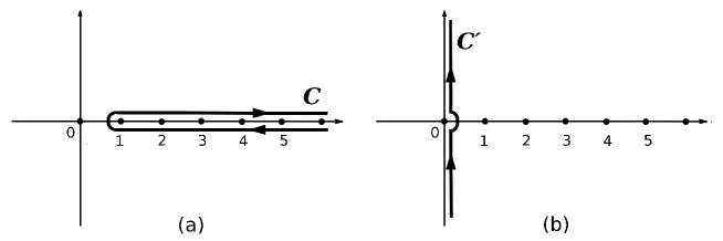
R ( 𝐲 , 𝐩 ) = lim λ → ∞ ∏ α = 1 M [ 1 2 i ∫ 𝒞 d z α sin ( π z α ) exp { λ z α y α } ] Φ [ 𝐩 , 𝐩 λ , λ 𝐳 ; 𝐳 ] 𝑅 𝐲 𝐩 subscript → 𝜆 superscript subscript product 𝛼 1 𝑀 delimited-[] 1 2 𝑖 subscript 𝒞 𝑑 subscript 𝑧 𝛼 𝜋 subscript 𝑧 𝛼 𝜆 subscript 𝑧 𝛼 subscript 𝑦 𝛼 Φ 𝐩 𝐩 𝜆 𝜆 𝐳 𝐳
R({\bf y},{\bf p})\;=\;\lim_{\lambda\to\infty}\prod_{\alpha=1}^{M}\Biggl{[}\frac{1}{2i}\int_{{\cal C}}\frac{dz_{\alpha}}{\sin(\pi z_{\alpha})}\exp\{\lambda z_{\alpha}y_{\alpha}\}\Biggr{]}\;\Phi\Bigl{[}{\bf p},\;\frac{{\bf p}}{\lambda},\;\lambda{\bf z};\;{\bf z}\Bigr{]} (72)
where the integration goes over the contour 𝒞 𝒞 {\cal C} 𝒞 ′ superscript 𝒞 ′ {\cal C}^{\prime} ∞ \infty z → z / λ → 𝑧 𝑧 𝜆 z\to z/\lambda λ → ∞ → 𝜆 \lambda\to\infty
R ( 𝐲 , 𝐩 ) = ∏ α = 1 M [ 1 2 π i ∫ 𝒞 ′ d z α z α exp { z α y α } ] lim λ → ∞ Φ [ 𝐩 , 𝐩 λ , 𝐳 ; 𝐳 λ ] 𝑅 𝐲 𝐩 superscript subscript product 𝛼 1 𝑀 delimited-[] 1 2 𝜋 𝑖 subscript superscript 𝒞 ′ 𝑑 subscript 𝑧 𝛼 subscript 𝑧 𝛼 subscript 𝑧 𝛼 subscript 𝑦 𝛼 subscript → 𝜆 Φ 𝐩 𝐩 𝜆 𝐳 𝐳 𝜆
R({\bf y},{\bf p})\;=\;\prod_{\alpha=1}^{M}\Biggl{[}\frac{1}{2\pi i}\int_{{\cal C}^{\prime}}\frac{dz_{\alpha}}{z_{\alpha}}\exp\{z_{\alpha}y_{\alpha}\}\Biggr{]}\;\lim_{\lambda\to\infty}\Phi\Bigl{[}{\bf p},\;\frac{{\bf p}}{\lambda},\;{\bf z};\;\frac{{\bf z}}{\lambda}\Bigr{]} (73)
where the parameters y α subscript 𝑦 𝛼 y_{\alpha} p α subscript 𝑝 𝛼 p_{\alpha} z α subscript 𝑧 𝛼 z_{\alpha} λ → ∞ → 𝜆 \lambda\to\infty
Figure 1: The contours of integration in the complex plane used for
summing the series:
(a) the original contour 𝒞 𝒞 {\cal C} 𝒞 ′ superscript 𝒞 ′ {\cal C}^{\prime}
Let us consider now the summations in eq.(69
∑ m α + s α ≥ 1 ∞ ( − 1 ) m α + s α − 1 f ( 𝐦 ; 𝐬 ) superscript subscript subscript 𝑚 𝛼 subscript 𝑠 𝛼 1 superscript 1 subscript 𝑚 𝛼 subscript 𝑠 𝛼 1 𝑓 𝐦 𝐬
\displaystyle\sum_{m_{\alpha}+s_{\alpha}\geq 1}^{\infty}(-1)^{m_{\alpha}+s_{\alpha}-1}\;f\bigl{(}{\bf m};{\bf s}\bigr{)} = \displaystyle= ∑ m α = 1 ∞ ( − 1 ) m α − 1 f ( 𝐦 ; 𝐬 ) | s α = 0 + ∑ s α = 1 ∞ ( − 1 ) s α − 1 f ( 𝐦 ; 𝐬 ) | m α = 0 − evaluated-at superscript subscript subscript 𝑚 𝛼 1 superscript 1 subscript 𝑚 𝛼 1 𝑓 𝐦 𝐬
subscript 𝑠 𝛼 0 limit-from evaluated-at superscript subscript subscript 𝑠 𝛼 1 superscript 1 subscript 𝑠 𝛼 1 𝑓 𝐦 𝐬
subscript 𝑚 𝛼 0 \displaystyle\sum_{m_{\alpha}=1}^{\infty}(-1)^{m_{\alpha}-1}\;f\bigl{(}{\bf m};{\bf s}\bigr{)}\big{|}_{s_{\alpha}=0}\;+\;\sum_{s_{\alpha}=1}^{\infty}(-1)^{s_{\alpha}-1}\;f\bigl{(}{\bf m};{\bf s}\bigr{)}\big{|}_{m_{\alpha}=0}\;-\; (74)
− \displaystyle- ∑ m α = 1 ∞ ( − 1 ) m α − 1 ∑ s α = 1 ∞ ( − 1 ) s α − 1 f ( 𝐦 ; 𝐬 ) superscript subscript subscript 𝑚 𝛼 1 superscript 1 subscript 𝑚 𝛼 1 superscript subscript subscript 𝑠 𝛼 1 superscript 1 subscript 𝑠 𝛼 1 𝑓 𝐦 𝐬
\displaystyle\sum_{m_{\alpha}=1}^{\infty}(-1)^{m_{\alpha}-1}\sum_{s_{\alpha}=1}^{\infty}(-1)^{s_{\alpha}-1}f\bigl{(}{\bf m};{\bf s}\bigr{)}
Thus, according to the above summation algorithm, we get
lim λ → ∞ ∑ m α + s α ≥ 1 ∞ ( − 1 ) m α + s α − 1 f ( 𝐦 ; 𝐬 ) = 1 ( 2 π i ) 2 ∫ ∫ 𝒞 ′ d z 1 α z 1 α d z 2 α z 2 α [ ( 2 π i ) δ ( z 2 α ) + ( 2 π i ) δ ( z 1 α ) − 1 ] lim λ → ∞ f ( 𝐳 1 λ ; 𝐳 2 λ ) subscript → 𝜆 superscript subscript subscript 𝑚 𝛼 subscript 𝑠 𝛼 1 superscript 1 subscript 𝑚 𝛼 subscript 𝑠 𝛼 1 𝑓 𝐦 𝐬
1 superscript 2 𝜋 𝑖 2 subscript superscript 𝒞 ′ 𝑑 subscript subscript 𝑧 1 𝛼 subscript subscript 𝑧 1 𝛼 𝑑 subscript subscript 𝑧 2 𝛼 subscript subscript 𝑧 2 𝛼 delimited-[] 2 𝜋 𝑖 𝛿 subscript subscript 𝑧 2 𝛼 2 𝜋 𝑖 𝛿 subscript subscript 𝑧 1 𝛼 1 subscript → 𝜆 𝑓 subscript 𝐳 1 𝜆 subscript 𝐳 2 𝜆
\lim_{\lambda\to\infty}\sum_{m_{\alpha}+s_{\alpha}\geq 1}^{\infty}(-1)^{m_{\alpha}+s_{\alpha}-1}\;f\bigl{(}{\bf m};{\bf s}\bigr{)}=\frac{1}{(2\pi i)^{2}}\int\int_{{\cal C}^{\prime}}\frac{d{z_{1}}_{\alpha}}{{z_{1}}_{\alpha}}\frac{d{z_{2}}_{\alpha}}{{z_{2}}_{\alpha}}\Bigl{[}(2\pi i)\delta({z_{2}}_{\alpha})+(2\pi i)\delta({z_{1}}_{\alpha})-1\Bigr{]}\lim_{\lambda\to\infty}f\Bigl{(}\frac{{\bf z}_{1}}{\lambda};\frac{{\bf z}_{2}}{\lambda}\Bigr{)} (75)
where the rescaled integration parameters
z 1 α subscript subscript 𝑧 1 𝛼 {z_{1}}_{\alpha} z 2 α subscript subscript 𝑧 2 𝛼 {z_{2}}_{\alpha} λ → ∞ → 𝜆 \lambda\to\infty Γ ( z ) | | z | → 0 = 1 / z evaluated-at Γ 𝑧 → 𝑧 0 1 𝑧 \Gamma(z)|_{|z|\to 0}=1/z Γ ( 1 + z ) | | z | → 0 = 1 evaluated-at Γ 1 𝑧 → 𝑧 0 1 \Gamma(1+z)|_{|z|\to 0}=1 𝒢 𝒢 {\cal G} 𝒢 α β subscript 𝒢 𝛼 𝛽 {\cal G}_{\alpha\beta} 61 62
lim λ → ∞ 𝒢 ( q α , m α , s α ) 2 ( m α + s α ) subscript → 𝜆 𝒢 subscript 𝑞 𝛼 subscript 𝑚 𝛼 subscript 𝑠 𝛼 superscript 2 subscript 𝑚 𝛼 subscript 𝑠 𝛼 \displaystyle\lim_{\lambda\to\infty}{\cal G}\bigl{(}q_{\alpha},m_{\alpha},s_{\alpha}\bigr{)}\;2^{(m_{\alpha}+s_{\alpha})} = \displaystyle= lim λ → ∞ 𝒢 ( p α λ , z 1 α λ , z 2 α λ ) 2 ( z 1 α / λ + z 2 α / λ ) subscript → 𝜆 𝒢 subscript 𝑝 𝛼 𝜆 subscript subscript 𝑧 1 𝛼 𝜆 subscript subscript 𝑧 2 𝛼 𝜆 superscript 2 subscript subscript 𝑧 1 𝛼 𝜆 subscript subscript 𝑧 2 𝛼 𝜆 \displaystyle\lim_{\lambda\to\infty}{\cal G}\Bigl{(}\frac{p_{\alpha}}{\lambda},\;\frac{{z_{1}}_{\alpha}}{\lambda},\;\frac{{z_{2}}_{\alpha}}{\lambda}\Bigr{)}2^{({z_{1}}_{\alpha}/\lambda+{z_{2}}_{\alpha}/\lambda)} (76)
= \displaystyle= ( z 1 α + z 2 α + i p α ( − ) ) ( z 1 α + z 2 α − i p α ( + ) ) ( z 2 α + i p α ( − ) ) ( z 1 α − i p α ( + ) ) ≡ 𝒢 ∗ ( p α , z 1 α , z 2 α ) subscript subscript 𝑧 1 𝛼 subscript subscript 𝑧 2 𝛼 𝑖 superscript subscript 𝑝 𝛼 subscript subscript 𝑧 1 𝛼 subscript subscript 𝑧 2 𝛼 𝑖 superscript subscript 𝑝 𝛼 subscript subscript 𝑧 2 𝛼 𝑖 superscript subscript 𝑝 𝛼 subscript subscript 𝑧 1 𝛼 𝑖 superscript subscript 𝑝 𝛼 subscript 𝒢 subscript 𝑝 𝛼 subscript subscript 𝑧 1 𝛼 subscript subscript 𝑧 2 𝛼 \displaystyle\frac{\bigl{(}{z_{1}}_{\alpha}+{z_{2}}_{\alpha}+ip_{\alpha}^{(-)}\bigr{)}\bigl{(}{z_{1}}_{\alpha}+{z_{2}}_{\alpha}-ip_{\alpha}^{(+)}\bigr{)}}{\bigl{(}{z_{2}}_{\alpha}+ip_{\alpha}^{(-)}\bigr{)}\bigl{(}{z_{1}}_{\alpha}-ip_{\alpha}^{(+)}\bigr{)}}\;\equiv\;{\cal G}_{*}\bigl{(}p_{\alpha},{z_{1}}_{\alpha},{z_{2}}_{\alpha}\bigr{)}
and
lim λ → ∞ 𝒢 α β ( 𝐩 λ , 𝐦 , 𝐬 ) = lim λ → ∞ 𝒢 α β ( 𝐩 λ , 𝐳 1 λ , 𝐳 2 λ ) = 1 subscript → 𝜆 subscript 𝒢 𝛼 𝛽 𝐩 𝜆 𝐦 𝐬 subscript → 𝜆 subscript 𝒢 𝛼 𝛽 𝐩 𝜆 subscript 𝐳 1 𝜆 subscript 𝐳 2 𝜆 1 \lim_{\lambda\to\infty}{\cal G}_{\alpha\beta}\Bigl{(}\frac{{\bf p}}{\lambda},\;{\bf m},\;{\bf s}\Bigr{)}\;=\;\lim_{\lambda\to\infty}{\cal G}_{\alpha\beta}\Bigl{(}\frac{{\bf p}}{\lambda},\;\frac{{\bf z}_{1}}{\lambda},\;\frac{{\bf z}_{2}}{\lambda}\Bigr{)}\;=\;1 (77)
where
p α ( ± ) = p α ± i ϵ superscript subscript 𝑝 𝛼 plus-or-minus plus-or-minus subscript 𝑝 𝛼 𝑖 italic-ϵ p_{\alpha}^{(\pm)}\;=\;p_{\alpha}\;\pm\;i\epsilon (78)
Thus, in the limit λ → ∞ → 𝜆 \lambda\to\infty 69
W ( f ) 𝑊 𝑓 \displaystyle W(f) = \displaystyle= 1 + ∑ M = 1 ∞ ( − 1 ) M M ! ∏ α = 1 M [ ∫ ∫ − ∞ + ∞ d y α d p α 2 π Ai ( y α + p α 2 − f ) \displaystyle 1+\sum_{M=1}^{\infty}\;\frac{(-1)^{M}}{M!}\;\prod_{\alpha=1}^{M}\Biggl{[}\int\int_{-\infty}^{+\infty}\frac{dy_{\alpha}dp_{\alpha}}{2\pi}\operatorname{Ai}\bigl{(}y_{\alpha}+p_{\alpha}^{2}-f\bigr{)} (79)
× \displaystyle\times 1 ( 2 π i ) 2 ∫ ∫ 𝒞 ′ d z 1 α z 1 α d z 2 α z 2 α [ ( 2 π i ) δ ( z 2 α ) + ( 2 π i ) δ ( z 1 α ) − 1 ] ( 1 + z 1 α z 2 α + i p α ( − ) ) ( 1 + z 2 α z 1 α − i p α ( + ) ) e ( z 1 α + z 2 α ) y α ] \displaystyle\frac{1}{(2\pi i)^{2}}\int\int_{{\cal C}^{\prime}}\frac{d{z_{1}}_{\alpha}}{{z_{1}}_{\alpha}}\frac{d{z_{2}}_{\alpha}}{{z_{2}}_{\alpha}}\Bigl{[}(2\pi i)\delta({z_{2}}_{\alpha})+(2\pi i)\delta({z_{1}}_{\alpha})-1\Bigr{]}\Bigl{(}1+\frac{{z_{1}}_{\alpha}}{{z_{2}}_{\alpha}+ip_{\alpha}^{(-)}}\Bigr{)}\Bigl{(}1+\frac{{z_{2}}_{\alpha}}{{z_{1}}_{\alpha}-ip_{\alpha}^{(+)}}\Bigr{)}\;\mbox{\LARGE e}^{({z_{1}}_{\alpha}+{z_{2}}_{\alpha})y_{\alpha}}\Biggr{]}
× \displaystyle\times det K ^ [ ( z 1 α , z 2 α , p α ) ; ( z 1 β , z 2 β , p β ) ] α , β = 1 , … , M ^ 𝐾 subscript subscript subscript 𝑧 1 𝛼 subscript subscript 𝑧 2 𝛼 subscript 𝑝 𝛼 subscript subscript 𝑧 1 𝛽 subscript subscript 𝑧 2 𝛽 subscript 𝑝 𝛽
formulae-sequence 𝛼 𝛽
1 … 𝑀
\displaystyle\det\hat{K}\bigl{[}({z_{1}}_{\alpha},{z_{2}}_{\alpha},p_{\alpha});({z_{1}}_{\beta},{z_{2}}_{\beta},p_{\beta})\bigr{]}_{\alpha,\beta=1,...,M}
= \displaystyle= det [ 1 − K ^ ] delimited-[] 1 ^ 𝐾 \displaystyle\det\bigl{[}1\,-\,\hat{K}\bigr{]}
with the kernel
K ^ [ ( z 1 , z 2 , p ) ; ( z 1 ′ , z 2 ′ , p ′ ) ] = 1 z 1 + z 2 − i p + z 1 ′ + z 2 ′ + i p ′ ^ 𝐾 subscript 𝑧 1 subscript 𝑧 2 𝑝 superscript subscript 𝑧 1 ′ superscript subscript 𝑧 2 ′ superscript 𝑝 ′
1 subscript 𝑧 1 subscript 𝑧 2 𝑖 𝑝 superscript subscript 𝑧 1 ′ superscript subscript 𝑧 2 ′ 𝑖 superscript 𝑝 ′ \hat{K}\bigl{[}({z_{1}},\,{z_{2}},\,p);({z_{1}}^{\prime},\,{z_{2}}^{\prime},\,p^{\prime})\bigr{]}\;=\;\frac{1}{{z_{1}}+{z_{2}}-ip+{z_{1}}^{\prime}+{z_{2}}^{\prime}+ip^{\prime}} (80)
In the exponential representation of this determinant we get
W ( f ) = exp [ − ∑ M = 1 ∞ 1 M Tr K ^ M ] 𝑊 𝑓 superscript subscript 𝑀 1 1 𝑀 Tr superscript ^ 𝐾 𝑀 W(f)\;=\;\exp\Bigl{[}-\sum_{M=1}^{\infty}\frac{1}{M}\;\mbox{Tr}\,\hat{K}^{M}\Bigr{]} (81)
where
Tr K ^ M Tr superscript ^ 𝐾 𝑀 \displaystyle\mbox{Tr}\,\hat{K}^{M} = \displaystyle= ∏ α = 1 M [ ∫ ∫ − ∞ + ∞ d y α d p α 2 π Ai ( y α + p α 2 − f ) × \displaystyle\prod_{\alpha=1}^{M}\Biggl{[}\int\int_{-\infty}^{+\infty}\frac{dy_{\alpha}dp_{\alpha}}{2\pi}\operatorname{Ai}\bigl{(}y_{\alpha}+p_{\alpha}^{2}-f\bigr{)}\times (82)
× \displaystyle\times 1 ( 2 π i ) 2 ∫ ∫ 𝒞 ′ d z 1 α z 1 α d z 2 α z 2 α [ ( 2 π i ) δ ( z 2 α ) + ( 2 π i ) δ ( z 1 α ) − 1 ] ( 1 + z 1 α z 2 α + i p α ( − ) ) ( 1 + z 2 α z 1 α − i p α ( + ) ) e ( z 1 α + z 2 α ) y α ] × \displaystyle\frac{1}{(2\pi i)^{2}}\int\int_{{\cal C}^{\prime}}\frac{d{z_{1}}_{\alpha}}{{z_{1}}_{\alpha}}\frac{d{z_{2}}_{\alpha}}{{z_{2}}_{\alpha}}\Bigl{[}(2\pi i)\delta({z_{2}}_{\alpha})+(2\pi i)\delta({z_{1}}_{\alpha})-1\Bigr{]}\Bigl{(}1+\frac{{z_{1}}_{\alpha}}{{z_{2}}_{\alpha}+ip_{\alpha}^{(-)}}\Bigr{)}\Bigl{(}1+\frac{{z_{2}}_{\alpha}}{{z_{1}}_{\alpha}-ip_{\alpha}^{(+)}}\Bigr{)}\;\mbox{\LARGE e}^{({z_{1}}_{\alpha}+{z_{2}}_{\alpha})y_{\alpha}}\Biggr{]}\times
× \displaystyle\times ∏ α = 1 M [ 1 z 1 α + z 2 α − i p α + z 1 α + 1 + z 2 α + 1 + i p α + 1 ] superscript subscript product 𝛼 1 𝑀 delimited-[] 1 subscript subscript 𝑧 1 𝛼 subscript subscript 𝑧 2 𝛼 𝑖 subscript 𝑝 𝛼 subscript subscript 𝑧 1 𝛼 1 subscript subscript 𝑧 2 𝛼 1 𝑖 subscript 𝑝 𝛼 1 \displaystyle\prod_{\alpha=1}^{M}\Biggl{[}\frac{1}{{z_{1}}_{\alpha}+{z_{2}}_{\alpha}-ip_{\alpha}+{z_{1}}_{\alpha+1}+{z_{2}}_{\alpha+1}+ip_{\alpha+1}}\Biggr{]}
Here, by definition, it is assumed that z i M + 1 ≡ z i 1 subscript 𝑧 subscript 𝑖 𝑀 1 subscript 𝑧 subscript 𝑖 1 {z_{i_{M+1}}}\equiv{z_{i_{1}}} i = 1 , 2 𝑖 1 2
i=1,2 p M + 1 ≡ p 1 subscript 𝑝 𝑀 1 subscript 𝑝 1 p_{M+1}\equiv p_{1}
1 z 1 α + z 2 α − i p α + z 1 α + 1 + z 2 α + 1 + i p α + 1 = ∫ 0 ∞ 𝑑 ω α exp [ − ( z 1 α + z 2 α − i p α + z 1 α + 1 + z 2 α + 1 + i p α + 1 ) ω α ] 1 subscript subscript 𝑧 1 𝛼 subscript subscript 𝑧 2 𝛼 𝑖 subscript 𝑝 𝛼 subscript subscript 𝑧 1 𝛼 1 subscript subscript 𝑧 2 𝛼 1 𝑖 subscript 𝑝 𝛼 1 superscript subscript 0 differential-d subscript 𝜔 𝛼 subscript subscript 𝑧 1 𝛼 subscript subscript 𝑧 2 𝛼 𝑖 subscript 𝑝 𝛼 subscript subscript 𝑧 1 𝛼 1 subscript subscript 𝑧 2 𝛼 1 𝑖 subscript 𝑝 𝛼 1 subscript 𝜔 𝛼 \frac{1}{{z_{1}}_{\alpha}+{z_{2}}_{\alpha}-ip_{\alpha}+{z_{1}}_{\alpha+1}+{z_{2}}_{\alpha+1}+ip_{\alpha+1}}\;=\;\int_{0}^{\infty}d\omega_{\alpha}\exp\Bigl{[}-\bigl{(}{z_{1}}_{\alpha}+{z_{2}}_{\alpha}-ip_{\alpha}+{z_{1}}_{\alpha+1}+{z_{2}}_{\alpha+1}+ip_{\alpha+1}\bigr{)}\,\omega_{\alpha}\Bigr{]} (83)
into eq.(82
Tr K ^ M = ∫ 0 ∞ 𝑑 ω 1 … 𝑑 ω M ∏ α = 1 M [ ∫ ∫ − ∞ + ∞ d y α d p α 2 π Ai ( y α + p α 2 + ω α + ω α − 1 − f ) exp { i p α ( ω α − ω α − 1 ) } S ( p α , y α ) ] Tr superscript ^ 𝐾 𝑀 superscript subscript 0 differential-d subscript 𝜔 1 … differential-d subscript 𝜔 𝑀 superscript subscript product 𝛼 1 𝑀 delimited-[] superscript subscript 𝑑 subscript 𝑦 𝛼 𝑑 subscript 𝑝 𝛼 2 𝜋 Ai subscript 𝑦 𝛼 superscript subscript 𝑝 𝛼 2 subscript 𝜔 𝛼 subscript 𝜔 𝛼 1 𝑓 𝑖 subscript 𝑝 𝛼 subscript 𝜔 𝛼 subscript 𝜔 𝛼 1 𝑆 subscript 𝑝 𝛼 subscript 𝑦 𝛼 \mbox{Tr}\,\hat{K}^{M}\;=\;\int_{0}^{\infty}d\omega_{1}\,...\,d\omega_{M}\,\prod_{\alpha=1}^{M}\Biggl{[}\int\int_{-\infty}^{+\infty}\frac{dy_{\alpha}dp_{\alpha}}{2\pi}\operatorname{Ai}\bigl{(}y_{\alpha}+p_{\alpha}^{2}+\omega_{\alpha}+\omega_{\alpha-1}-f\bigr{)}\exp\{ip_{\alpha}\bigl{(}\omega_{\alpha}-\omega_{\alpha-1}\bigr{)}\}\;S\bigl{(}p_{\alpha},\,y_{\alpha}\bigr{)}\Biggr{]} (84)
where, by definition, ω 0 ≡ ω M subscript 𝜔 0 subscript 𝜔 𝑀 \omega_{0}\equiv\omega_{M}
S ( p , y ) = 1 ( 2 π i ) 2 ∫ ∫ 𝒞 ′ d z 1 z 1 d z 2 z 2 [ ( 2 π i ) δ ( z 2 ) + ( 2 π i ) δ ( z 1 ) − 1 ] ( 1 + z 1 z 2 + i p ( − ) ) ( 1 + z 2 z 1 − i p ( + ) ) e ( z 1 + z 2 ) y α 𝑆 𝑝 𝑦 1 superscript 2 𝜋 𝑖 2 subscript superscript 𝒞 ′ 𝑑 subscript 𝑧 1 subscript 𝑧 1 𝑑 subscript 𝑧 2 subscript 𝑧 2 delimited-[] 2 𝜋 𝑖 𝛿 subscript 𝑧 2 2 𝜋 𝑖 𝛿 subscript 𝑧 1 1 1 subscript 𝑧 1 subscript 𝑧 2 𝑖 superscript 𝑝 1 subscript 𝑧 2 subscript 𝑧 1 𝑖 superscript 𝑝 superscript e subscript 𝑧 1 subscript 𝑧 2 subscript 𝑦 𝛼 S\bigl{(}p,\,y\bigr{)}\;=\;\frac{1}{(2\pi i)^{2}}\int\int_{{\cal C}^{\prime}}\frac{dz_{1}}{z_{1}}\,\frac{dz_{2}}{z_{2}}\Bigl{[}(2\pi i)\delta(z_{2})+(2\pi i)\delta(z_{1})-1\Bigr{]}\Bigl{(}1+\frac{z_{1}}{z_{2}+ip^{(-)}}\Bigr{)}\Bigl{(}1+\frac{z_{2}}{z_{1}-ip^{(+)}}\Bigr{)}\;\mbox{\LARGE e}^{(z_{1}+z_{2})y_{\alpha}} (85)
Simple calculations yield:
S ( p , y ) 𝑆 𝑝 𝑦 \displaystyle S\bigl{(}p,\,y\bigr{)} = \displaystyle= 1 2 π i ∫ 𝒞 ′ d z 1 z 1 ( 1 + z 1 i ( p − i ϵ ) ) exp { z 1 y } + 1 2 π i ∫ 𝒞 ′ d z 2 z 2 ( 1 − z 2 i ( p + i ϵ ) ) exp { z 2 y } − 1 2 𝜋 𝑖 subscript superscript 𝒞 ′ 𝑑 subscript 𝑧 1 subscript 𝑧 1 1 subscript 𝑧 1 𝑖 𝑝 𝑖 italic-ϵ subscript 𝑧 1 𝑦 limit-from 1 2 𝜋 𝑖 subscript superscript 𝒞 ′ 𝑑 subscript 𝑧 2 subscript 𝑧 2 1 subscript 𝑧 2 𝑖 𝑝 𝑖 italic-ϵ subscript 𝑧 2 𝑦 \displaystyle\frac{1}{2\pi i}\int_{{\cal C}^{\prime}}\frac{dz_{1}}{z_{1}}\,\Bigl{(}1+\frac{z_{1}}{i(p-i\epsilon)}\Bigr{)}\,\exp\{z_{1}y\}\;+\;\frac{1}{2\pi i}\int_{{\cal C}^{\prime}}\frac{dz_{2}}{z_{2}}\,\Bigl{(}1-\frac{z_{2}}{i(p+i\epsilon)}\Bigr{)}\,\exp\{z_{2}y\}\;- (86)
− \displaystyle- 1 ( 2 π i ) 2 ∫ ∫ 𝒞 ′ d z 1 z 1 d z 2 z 2 ( 1 + z 1 z 2 + i ( p − i ϵ ) ) ( 1 + z 2 z 1 − i ( p + i ϵ ) ) exp { ( z 1 + z 2 ) y } 1 superscript 2 𝜋 𝑖 2 subscript superscript 𝒞 ′ 𝑑 subscript 𝑧 1 subscript 𝑧 1 𝑑 subscript 𝑧 2 subscript 𝑧 2 1 subscript 𝑧 1 subscript 𝑧 2 𝑖 𝑝 𝑖 italic-ϵ 1 subscript 𝑧 2 subscript 𝑧 1 𝑖 𝑝 𝑖 italic-ϵ subscript 𝑧 1 subscript 𝑧 2 𝑦 \displaystyle\frac{1}{(2\pi i)^{2}}\int\int_{{\cal C}^{\prime}}\frac{dz_{1}}{z_{1}}\,\frac{dz_{2}}{z_{2}}\Bigl{(}1+\frac{z_{1}}{z_{2}+i(p-i\epsilon)}\Bigr{)}\Bigl{(}1+\frac{z_{2}}{z_{1}-i(p+i\epsilon)}\Bigr{)}\exp\{(z_{1}+z_{2})y\}
= \displaystyle= [ 1 i ( p − i ϵ ) − 1 i ( p + i ϵ ) ] δ ( y ) delimited-[] 1 𝑖 𝑝 𝑖 italic-ϵ 1 𝑖 𝑝 𝑖 italic-ϵ 𝛿 𝑦 \displaystyle\Bigl{[}\frac{1}{i(p-i\epsilon)}-\frac{1}{i(p+i\epsilon)}\Bigr{]}\;\delta(y)
Taking the limit ϵ → 0 → italic-ϵ 0 \epsilon\to 0
S ( p , y ) = δ ( y ) δ ( p ) 𝑆 𝑝 𝑦 𝛿 𝑦 𝛿 𝑝 S\bigl{(}p,\,y\bigr{)}\;=\;\delta(y)\delta(p) (87)
Substituting this result into eq.(84
Tr K ^ M = ∫ 0 ∞ 𝑑 ω 1 … 𝑑 ω M ∏ α = 1 M [ Ai ( ω α + ω α − 1 − f ) ] Tr superscript ^ 𝐾 𝑀 superscript subscript 0 differential-d subscript 𝜔 1 … differential-d subscript 𝜔 𝑀 superscript subscript product 𝛼 1 𝑀 delimited-[] Ai subscript 𝜔 𝛼 subscript 𝜔 𝛼 1 𝑓 \mbox{Tr}\,\hat{K}^{M}\;=\;\int_{0}^{\infty}d\omega_{1}\,...\,d\omega_{M}\,\prod_{\alpha=1}^{M}\Bigl{[}\operatorname{Ai}\bigl{(}\omega_{\alpha}+\omega_{\alpha-1}-f\bigr{)}\Bigr{]} (88)
In other words, the free energy distribution function of our problem
is given by the Fredholm determinant,
W ( f ) = det [ 1 − K ^ − f ] 𝑊 𝑓 delimited-[] 1 subscript ^ 𝐾 𝑓 W(f)\;=\;\det\Bigl{[}1\;-\;\hat{K}_{-f}\Bigr{]} (89)
with the kernel
K − f ( ω , ω ′ ) = Ai ( ω + ω ′ − f ) , ( ω , ω ′ > 0 ) subscript 𝐾 𝑓 𝜔 superscript 𝜔 ′ Ai 𝜔 superscript 𝜔 ′ 𝑓 𝜔 superscript 𝜔 ′
0
K_{-f}(\omega,\omega^{\prime})\;=\;\operatorname{Ai}\bigl{(}\omega\;+\;\omega^{\prime}\;-\;f\bigr{)}\;,\;\;\;\;\;\;\;\;\;\;\;\;\;\;\;\;(\omega,\;\omega^{\prime}\;>\;0) (90)
which is the GOE Tracy-Widom distribution TW2 ; Ferrari-Spohn
IV Conclusions
In this paper we have presented sufficiently simple derivation of the
GOE Tracy-Widom distribution function for the free energy fluctuations in
random directed polymers with free boundary conditions.
The main message of this somewhat technical work is not
the final result itself (which is not new anyway), but the demonstration
of the efficiency of the general method and new
technical tricks used in the derivation.
By mapping the original problem to the N 𝑁 N
The key technical tricks of presented calculations includes the following points.
First of all, to make the integration over particle coordinates of the Bethe ansatz
propagator well defined one has to introduce proper
regularization at ± ∞ plus-or-minus \pm\infty + ∞ +\infty − ∞ -\infty 15 16 37 43 49 t → ∞ → 𝑡 t\to\infty 71 73 76 77 79
Hopefully, the experience obtained in the presented calculations would help
to solve more serious long standing problems of this scope, such as
the distribution function of the directed polymer’s end point fluctuations or
the statistical properties of the free energy fluctuations at different times.
Acknowledgements. An essential part of this work was done
during my visit to the Fields Institute, Toronto, in the spring of 2011
in the framework of the program ”Dynamics and transport in disordered systems”.
I would like to thank Jeremy Quastel and Kostya Khanin for numerous
illuminating discussions which were crucial for the progress in these somewhat
complicated calculations.
This work was supported in part by the grant IRSES DCPA PhysBio-269139.