logcf: An Efficient Tool for Real Root Isolation

Abstract

This paper revisits an algorithm for isolating real roots of univariate polynomials based on continued fractions. It follows the work of Vincent, Uspensky, Collins and Akritas, Johnson and Krandick. We use some tricks, especially a new algorithm for computing an upper bound of positive roots. In this way, the algorithm of isolating real roots is improved. The complexity of our method for computing an upper bound of positive roots is $O(n\log(u+1))$ where $u$ is the optimal upper bound satisfying Theorem 3 and $n$ is the degree of the polynomial. Our method has been implemented as a software package logcf using C++ language. For many benchmarks logcf  is two or three times faster than the function RootIntervals of Mathematica. And it is much faster than another continued fractions based software CF, which seems to be one of the fastest available open software for exact real root isolation. For those benchmarks which have only real roots, logcf is much faster than Sleeve and eigensolve which are based on numerical computation.

1 Introduction

Real root isolation of univariate polynomials with integer coefficients is one of the fundamental tasks in computer algebra as well as in many applications ranging from computational geometry to quantifier elimination. The problem can be stated as: given a polynomial $P\in{\mathbb{Z}}[x]$, compute for each of its real roots an interval with rational endpoints containing it and being disjoint from the intervals computed for the other roots. The methods of isolating real root can be divided into three kinds. The first kind consists of the subdivision algorithms using counting techniques based on, e.g., the Strum theorem or Descartes’ rule of signs. This kind of methods count the sign changes (of Sturm sequence or coefficients of some polynomials) in the considered interval and if the sign changes reach $1$ or $0$, the procedure returns from this interval. Otherwise it subdivides the interval and compute recursively. The symbolic implementations of these methods can be found in [5, 18] and the symbolic-numberic algorithms implementations can be found in [18, 7, 6, 16].

The second kind takes use of the continued fraction (CF) algorithms [4, 22, 20]. These methods are highly efficient and competitive [18, 2, 11]. Especially, [11] provides a test datasets consisting of 5000 polynomials from many different settings, with results indicating that there is no best method overall. However one can say that for most instances the solvers based on CF are among the best methods. In this paper we modify a real root isolation algorithm based on CF method to obtain a more efficient tool logcf.

The third kind is based on Newton-Raphson method and interval arithmetic. The search space is subdivided until it contains only a single real root and Newton’s method converges. When the polynomial is sparse and has very high degree, this method will be much faster than other methods. The symbolic implementations of this kind of methods can be found in [23, 24] and the numeric implementations can be found in [15, 19].

Those methods based on CF compute the continued fraction expansion of the real roots of a polynomial in order to compute isolating intervals for real roots. One important step is the computation of upper bounds of the positive real roots of some polynomials. There are several classic methods to compute such upper bounds, such as Cauchy bounds, Lagrange-MacLaurin bounds and Kioustelidis’ bounds. There are many recent works about the upper bound of the positive roots of univariate polynomials [12, 21, 2, 3, 4]. Some methods for computing such bounds are of $O(n)$ complexity but the results are very coarse like Cauchy bounds. Some methods are of $O(n^{2})$ complexity but their bounds are sharper such as the method presented in [4]. The balance between precision and effect for computing such upper bounds has to be taken into account.

We provide a new method for computing such bounds with time complexity $O(n\log(u+1))$, where $u$ is the optimal upper bound satisfying Theorem 3. Besides, compared with [4], when Algorithm 5 return true (the upper bound is less than $1$), our upper bound is at most two times that in [4]. In this way, the algorithm of isolating real roots is improved. Our method has been implemented as a software package logcf using C++ language. For many benchmarks logcf  is two or three times faster than the function RootIntervals of Mathematica. And it is much faster than another continued fractions based software CF, which seems to be one of the fastest available open software for exact real root isolation. For those benchmarks which have only real roots, logcf is much faster than Sleeve and eigensolve which are based on numerical computation.

The rest of this paper is organized as follows. Section 2 reviews the main algorithm for real root isolation based on CF. Section 3 presents a new algorithm for computing an upper bound of positive roots. Section 4 lists some tricks used in logcf. Section 5 lists the comparative experimental results of our algorithm and other software.

2 Algorithm based on CF

In this section, we first recall Descartes’ rule of signs, which gives a bound on the number of positive real roots. Then the Vincent theorem, which can ensure the termination of algorithms based on CF, is presented. Finally, we review an algorithm of real root isolation based on CF.

As usual, ${\rm deg}(p)$ denotes the degree of univariate polynomial $p$. The derivative of polynomial $p$ with respect to the only variable is denoted by $p^{\prime}$ and ${\rm gcd}(f,g)$ means the greatest common divisor of polynomials $f$ and $g$.

Notation 1 (Sign variation).

Let $S=\left\{a_{0},a_{1},\ldots,a_{n}\right\}$ be a finite sequence of non-zero real numbers. Define $V(S)$, the sign variation of $S$, as follows.

$$V(S)=0\ \text{ if }|S|\leq 1,$$

$$V(a_{0},\ldots,a_{n-1},a_{n})=\left\{\begin{aligned} &V(a_{0},\ldots,a_{n-1})+1\text{ if }a_{n-1}a_{n}<0;\\ &V(a_{0},\ldots,a_{n-1}),\text{ otherwise}.\\ \end{aligned}\right.$$

If some elements of $S$ are zero, remove those zero-elements to get a new sequence and define $V(S)$ to be the sign variation of this new sequence.

Theorem 1 (Descartes’ rule of signs).

Suppose $p=\sum_{i=0}^{n}a_{i}x^{i}\in{\mathbb{R}}[x]$ has $m$ positive real roots, counted with multiplicity. Set $V(p)=V(a_{0},a_{1},\ldots,a_{n})$. Then $m\leq V(p)$, and $V(p)-m$ is even.

Theorem 2 (Vincent’s theorem).

Let $P(x)$ be a real polynomial of degree $n$ which has only simple roots. It is possible to determine a positive quantity $\delta$ so that for every pair of positive real numbers $a$ and $b$ with $|b-a|<\delta$, the coefficients sequence of every transformed polynomial of the form $P(x)=(1+x)^{n}P(\frac{a+bx}{1+x})$ has exactly 0 or 1 sign variation. The second case is possible if and only if $P(x)$ has a single root within $(a,b)$.

Input: A non-zero polynomial $P(x)\in{\mathbb{Z}}[x]$.

Output: $I$, a set of real root isolating intervals of $P(x)$.

1 $I=\emptyset$;

2 if ${\rm deg}(P)==0$ then

3      return $I$;

$P=\frac{P}{{\rm gcd}(P,P^{\prime})}$; /* square free */

4 if $P(0)==0$  then

       $I.add([0,0])$; /* add $[0,0]$ to set $I$ */

       dec($P$); /* Algorithm 2 */

5      

6$I$.addAll(cf($P$));

/* add all the positive root intervals to set $I$ */

/* cf is described as Algorithm 4 */

7 $p=-p$;

$I$.addAll(cf($P$));

Algorithm 1 main

CF based procedures will continue subdividing the considered interval into two subintervals and make a one to one map from $(a,b)$ to $(0,+\infty)$ by $P(x)=(1+x)^{n}P(\frac{a+bx}{1+x})$ until $V(P)$ equals $1$ or $0$. Therefore, Theorem 2 guarantees the termination of these procedures.

Definition 1.

As in [2], we define the following transformations for a univariate polynomial $P(x)$.

$$R(P(x))=x^{n}(P(\frac{1}{x})),$$

$$H_{\lambda}(P(x))=P(\lambda x),$$

$$T(P(x))=P(x+1).$$

$T(P)$ is also called Taylor shift one [9, 14]. In our experiments when Algorithm 6 is used for computing upper bounds, $T(P)$ takes more than ninety percent of running time. We have considered methods in [9] for computing $T(P)$, but finally we chose the classical method (Horner’s method) for its simplicity. In future work we will use Divide & Conquer method which is the fastest in [9]. We think this substituting will still improve the performance of our method.

Input: $P=a_{n}x^{n}+a_{n-1}x^{n-1}+\cdots+a_{1}x+a_{0},n>0$.

Output: $P=a_{n}x^{n-1}+a_{n-1}x^{n-2}+\cdots+a_{2}x+a_{1}$ .

Algorithm 2 dec

Input: $P\in{\mathbb{Z}}[x]$.

Output: $root\_lb$, a lower bound of positive roots of $P$.

1 $P=R(P)$;

$root\_lb=$logup($P$); /* logup is described as Algorithm 6 */

Algorithm 3 loglb

Definition 2.

$intvl(a,b,c,d)=\left\{\begin{aligned} &(\min\left\{\frac{a}{c},\frac{b}{d}\right\},\max\left\{\frac{a}{c},\frac{b}{d}\right\})&\text{ if }cd\neq 0;\\ &(0,\infty),&\text{ otherwise}.\\ \end{aligned}\right.$

Using the above notations and definitions, an algorithm for isolating all the real roots of a nonzero univariate polynomial is described as Algorithm 1. Algorithm 4, which has only a little modification of the algorithm in [4], is presented here to make our subsequent description clearer.

3 A new algorithm of computing upper bounds

One key ingredient of CF based methods is the computation of upper bounds of the positive real roots of some polynomials. We give in Theorem 3 a new characteristic of such upper bounds of univariate polynomials. A new algorithm based on this theorem, Algorithm 6, is proposed for computing upper bounds of positive real roots.

Input: A squarefree polynomial $F\in{\mathbb{Z}}[x]\setminus\{0\}$.

Output: $roots$, a list of isolating intervals of positive roots of $F$.

1

2$roots=\emptyset$; $s=V(F)$;

3

4$intstack=\emptyset$; $intstack$.add($\{1,0,0,1,F,s\}$);

5

6while $intstack\neq\emptyset$ do

       $\{a,b,c,d,P,s\}=intstack.$pop();/* pop the first element */

7       $\alpha={\tt loglb}(P)$;

8       if $\alpha\geq 1$  then

9             $\{a,c,P\}=\{\alpha a,\alpha c,H_{\alpha}(P)\}$; $\{b,d,P\}=\{a+b,c+d,T(P)\}$;

10            if  $P(0)==0$ then

11                   $roots$.add$([\frac{b}{d},\frac{b}{d}])$ ; $P=\frac{P}{x}$;

12                  

13            $s=V(P)$;

14             if $s==0$ then

15                   continue;

16                  

17            else if $s==1$ then

18                  

19                  $roots$.add($intvl(a,b,c,d)$); continue;

20                  

21            

22      $\left\{P_{1},a_{1},b_{1},c_{1},d_{1},r\right\}=\left\{T(P),a,a+b,c,c+d,0\right\}$

23      if $P_{1}(0)==0$ then

24             $roots$.add($[\frac{b_{1}}{d_{1}},\frac{b_{1}}{d_{1}}]$); $P_{1}=\frac{P_{1}}{x};r=1$;

25            

26      $s_{1}=V(P_{1})$; $\left\{s_{2},a_{2},b_{2},c_{2},d_{2}\right\}=\left\{s-s_{1}-r,b,a+b,d,c+d\right\}$;

27      if $s_{2}>1$  then

28             $P_{2}=(x+1)^{{\rm deg}(P)}T(P)$;

29             if $P_{2}(0)==0$ then

30                   $P_{2}=\frac{P_{2}}{x}$; $s_{2}=V(P_{2})$;

31                  

32            

33      if $s_{1}==1$  then

34            

35            $roots$.add($intvl(a_{1},b_{1},c_{1},d_{1})$);

36            

37      else if $s_{1}>1$  then

38            

39            $intstack$.add($\{a_{1},b_{1},c_{1},d_{1},P_{1},s_{1}\}$);

40            

41      

42      if $s_{2}==1$ then

43            

44            $roots$.add($intvl(a_{2},b_{2},c_{2},d_{2})$);

45            

46      else if $s_{2}>1$  then

47            

48            $intstack$.add($\{a_{2},b_{2},c_{2},d_{2},P_{2},s_{2}\}$);

49            

50      

Algorithm 4 cf

Theorem 3.

Suppose $P=a_{n}x^{n}+a_{n-1}x^{n-1}+\cdots+a_{1}x+a_{0}\ (a_{n}>0)$ is a univariate polynomial in $x$ with real coefficients. Then a nonnegative number $u$ is an upper bound of positive roots of $P$ if $u$ satisfies $\min_{j=0}^{n}\left\{\sum_{i=j}^{n}a_{i}u^{i-j}\right\}\geq 0$.

Proof 1.

If $n==0$, then $P$ is a nonzero constant and any positive number is its upper bound of positive roots.

Otherwise, if $b>u$, we claim that $\sum_{i=j}^{n}a_{i}b^{i-j}>\sum_{i=j}^{n}a_{i}u^{i-j}$ for any $j=0,\ldots,n-1$.

When $j=n-1$, $\sum_{i=n-1}^{n}a_{i}b^{i-n+1}-\sum_{i=n-1}^{n}a_{i}u^{i-n+1}=a_{n}(b-u)>0.$ The claim holds.

Assume the claim holds when $j=k$. When $j=k-1$, $\sum_{i=k-1}^{n}a_{i}b^{i-k+1}=\left(\sum_{i=k}^{n}a_{i}b^{i-k}\right)b+a_{k-1}$. By assumption $\sum_{i=k}^{n}a_{i}b^{i-k}>\sum_{i=k}^{n}a_{i}u^{i-k}\geq 0$. Since $b>u\geq 0$, $\left(\sum_{i=k}^{n}a_{i}b^{i-k}\right)b>\left(\sum_{i=k}^{n}a_{i}u^{i-k}\right)u$ and $\sum_{i=k-1}^{n}a_{i}b^{i-k+1}>\sum_{i=k-1}^{n}a_{i}u^{i-k+1}$. So $\sum_{i=j}^{n}a_{i}b^{i-j}>\sum_{i=j}^{n}a_{i}u^{i-j}$ for any $j=0,\ldots,n-1$.

By the above claim, $P(b)=\sum_{i=0}^{n}a_{i}b^{i}>0$ when $b>u$. Because $b$ is arbitrarily chosen, $u$ is an upper bound of the positive roots of $P$.

The following theorem was given by Akritas et al. in [3, 4], which computes positive root upper bounds of univariate polynomials.

Theorem 4 (Akritas-Strzeboński-Vigklas, [3]).

Let $P(x)=a_{n}x^{n}+a_{n-1}x^{n-1}+\cdots+a_{0}\ (a_{n}>0)$ be a polynomial with real coefficients and let $d(P)$ and $t(P)$ denote the degree and the number of its terms, respectively.

Moreover, assume that $P(x)$ can be written as

$$P(x)=q_{1}(x)-q_{2}(x)+q_{3}(x)-q_{4}(x)+\cdots+q_{2m-1}(x)-q_{2m}(x)+g(x)$$ (1)

where all the coefficients of polynomials $q_{i}(x)$ $(i=1,2,\ldots,2m)$ and $g(x)$ are positive. In addition, assume that for $i=1,2,\ldots,m$ we have

$$q_{2i-1}(x)=c_{2i-1,1}x^{e_{2i-1,1}}+\cdots+c_{2i-1,t_{2i-1}}x^{e_{2i-1,t_{2i-1}}}$$

and

$$q_{2i}(x)=b_{2i,1}x^{e_{2i,1}}+\cdots+b_{2i,t_{2i}}x^{e_{2i,t_{2i}}}$$

where $e_{2i-1,1}=d(q_{2i-1})$, $e_{2i,1}=d(q_{2i})$, $t_{2i-1}=t(q_{2i-1}),$ and $t_{2i}=t(q_{2i})$ and the exponent of each term in $q_{2i-1}(x)$ is greater than the exponent of each term in $q_{2i}(x)$. If for all indices $i=1,2,\ldots,m$, we have

$$t(q_{2i-1})\geq t(q_{2i}),$$

then an upper bound of the values of the positive roots of $p(x)$ is given by

$$up=\max_{i=1,2,\ldots,m}\left\{\max_{j=1,2,\ldots,t_{2i}}\left\{\left(\frac{b_{2i,j}}{c_{2i-1,j}}\right)^{\frac{1}{e_{2i-1,j}-e_{2i,j}}}\right\}\right\}$$ (2)

for any permutation of the positive coefficients $c_{2i-1,j},$ $j=1,2,\ldots,t_{2i-1}$. Otherwise, for each of the indices $i$ for which we have

$$t_{2i-1}<t_{2i},$$

we break up one of the coefficients of $q_{2i-1}(x)$ into $t_{2i}-t_{2i-1}+1$ parts, so that now $t(q_{2i})=t(q_{2i-1})$ and apply the same formula (2) given above.

We shall show in Theorem 6 that the bound given by Theorem 3 is better than that given by Theorem 4.

Theorem 5.

Let $P(x)=a_{n}x^{n}+a_{n-1}x^{n-1}+\cdots+a_{0}\ (a_{n}>0)$ be a polynomial with real coefficients and $u$ denote an upper bound of positive roots of $p$ obtained by Theorem 4, then $\min_{k=0}^{n}\left\{\sum_{i=k}^{n}a_{i}u^{i-k}\right\}\geq 0$.

Proof 2.

For every $a_{i}<0$, by Theorem 4, there exist $c_{i_{1}}x^{e_{i_{1}}}$ and $b_{i_{2}}x^{e_{i_{2}}},$ respectively, such that $e_{i_{1}}>e_{i_{2}}$ and $c_{i_{1}}u^{e_{i_{1}}}\geq b_{i_{2}}u^{e_{i_{2}}}$. By Theorem 4 $b_{i_{2}}x^{e_{i_{2}}}$ is the term $-a_{i}x^{i}$ and $c_{i_{1}}x^{e_{i_{1}}}$ is either a whole or a part (broken up by Theorem 4) of a positive term of $p$.

For every $a_{j}>0$, by Theorem 4, $\left(\sum_{a_{i}<0,e_{i_{1}}=j}c_{i_{1}}\right)\leq a_{j}$. So $\sum_{i=k}^{n}a_{i}u^{i}\geq\sum_{i=k,a_{i}<0}^{n}\left(c_{i_{1}}u^{e_{i_{1}}}-b_{i_{2}}u^{e_{i_{2}}}\right)\geq 0$ for any $k=0,1,\ldots,n$. Then $\sum_{i=k}^{n}a_{i}u^{i-k}\geq 0$ for any $k=0,1,\ldots,n$ and $\min_{k=0}^{n}\left\{\sum_{i=k}^{n}a_{i}u^{i-k}\right\}\geq 0$.

Theorem 6.

Let $P(x)=a_{n}x^{n}+a_{n-1}x^{n-1}+\cdots+a_{0}\ (a_{n}>0)$ be a polynomial with real coefficients. Let $u_{1}$ denote the optimal upper bound of positive real roots satisfying Theorem 3 and $u_{2}$ denote the optimal upper bound of positive real roots satisfying Theorem 4, then $u_{1}\leq u_{2}$ and the strict inequality can hold.

Proof 3.

By Theorem 5, $u_{1}\leq u_{2}$.

Let $P(x)=x^{2}+x-2$. Then $u_{2}=\sqrt{2}$ and $u_{1}=1$. So $u_{1}<u_{2}$ for this $P$.

Theorem 7.

Let $P(x)=a_{n}x^{n}+a_{n-1}x^{n-1}+\cdots+a_{0}\ (V(P)>0)$ be a polynomial with real coefficients. Let $u$ denote the output of Algorithm 6 and $u_{1}$ denote the optimal upper bound of $P$ satisfying Theorem 3. When $u$ is less than or equal to $1$, $u<2u_{1}$.

Input: $P=a_{n}x^{n}+a_{n-1}x^{n-1}+\cdots+a_{1}x+a_{0}\in{\mathbb{Z}}[x],\exists a_{i},a_{n}a_{i}<0$.

Output: true: the positive root bound of $P$ must be less than $1$;

               false: cannot determine whether the bound is less than $1$.

1

2$start=n-1$;

3 $lastNeg=0$;

4 $hSign={\rm sign}(a_{n})$;

5

6while ${\rm sign}(a_{lastNeg})+hSign\neq 0$  do

7       $lastNeg=lastNeg+1$;

8      

9

10while ${\rm sign}(a_{start})+hSign\neq 0$  do

11       $start=start-1$;

12      

13$cfSum={\rm abs}(a_{n})$;

14 $i=n-1$;

15 $j=start$;

16 $last=start$;

17 while $i\geq lastNeg-1\text{ and }j\geq lastNeg-1$ do

18       if ${\rm sign}(cfSum)<0$ then

19             while $i>last\text{ and }{\rm sign}(a_{i})\neq hSign$  do

20                   $i=i-1$;

21            

22            if $i==last$ then

23                   return false;

24            $cfSum=cfSum+{\rm abs}(a_{i})$;

25             $i=i-1$;

26            

27      else

28             if $j==lastNeg-1$  then

29                   return true;

30            while $j\geq lastNeg\text{ and }{\rm sign}(a_{j})+hSign\neq 0$  do

31                   $j=j-1$;

32            $cfSum=cfSum-{\rm abs}(a_{j})$;

33             $last=j$;

34            

35      

36

37return true;

Algorithm 5 lessOne

Input: $P=a_{n}x^{n}+a_{n-1}x^{n-1}+\cdots+a_{1}x+a_{0}\in{\mathbb{Z}}[x],\exists a_{i},a_{n}a_{i}<0.$

Output: an upper bound of the positive roots of $P$.

1 $start=n-1$; $lastNeg=0$; $hSign={\rm sign}(a_{n})$; $base=1$;

2

3if $\neg$lessOne($P$)  then

4       return $2$;

5while ${\rm sign}(a_{lastNeg})+hSign\neq 0$  do

6       $lastNeg=lastNeg+1$;

7      

8

9while ${\rm sign}(a_{start})+hSign\neq 0$  do

10       $start=start-1$;

11      

12

13$i=n$;

14 while $i==n$ do

15      

16      $i=n-1$;

17       $j=start$;

18       $cfSum={\rm abs}(a_{n})$;

19      

20      while $i\geq lastNeg-1\text{ and }j\geq lastNeg-1$ do

21             if ${\rm sign}(cfSum)<0$ then

22                   while $i>j\text{ and }{\rm sign}(a_{i})\neq hSign$  do

23                         $i=i-1$;

24                  if $i==j$ then

25                         break;

26                  $cfSum=cfSum+{\rm abs}(a_{i})2^{(n-i)base}$;

27                   $i=i-1$;

28                  

29            else

30                  

31                  if $j==lastNeg-1$  then

32                         $j=lastNeg-2$; break;

33                        

34                  

35                  while $j\geq lastNeg\text{ and }{\rm sign}(a_{j})+hSign\neq 0$  do

36                         $j=j-1$;

37                  

38                  $cfSum=cfSum-{\rm abs}(a_{i})2^{(n-j)base}$;

39                  

40                  $j=j-1$;

41                  

42            

43      if $j==lastNeg-2$ then

44             $base=base+1$; $i=n$;

45            

46      

47return $\frac{1}{2^{base-1}}$;

Algorithm 6 logup

Proof 4.

In Algorithm 6, if $\frac{1}{2^{base}}\geq u_{1},$ then $\min_{j=0}^{n}\left\{\sum_{i=j}^{n}a_{i}\left({\frac{1}{2^{base}}}\right)^{i-j}\right\}\geq 0$ by the proof of Theorem 3 and thus the loop does not terminate at this step. So when Algorithm 6 returns, $base$ must satisfy $\frac{1}{2^{base}}<u_{1}$. Therefore, the output $u=\frac{1}{2^{base-1}}$ and $u<2u_{1}$. Obviously, this algorithm will terminate.

Furthermore, $\min_{j=0}^{n-1}\left\{\sum_{i=j}^{n}a_{i}\left({\frac{1}{2^{base-1}}}\right)^{i-j}\right\}\geq 0$ by Theorem 3. So, $u=\frac{1}{2^{base-1}}$ is an upper bound of $p$.

Corollary 8.

Let $P(x)=a_{n}x^{n}+a_{n-1}x^{n-1}+\cdots+a_{0}$ $(V(P)>0)$ be a polynomial with real coefficients. Set $u$ to be the optimal upper bound of positive roots of $P$ satisfying Theorem 3. Then Algorithm 6 costs at most $O(n\log(u+1))$ additions and multiplications.

4 Tricks

Variable substitution If $P(x)\in{\mathbb{Z}}[x]$ and $P(x)=P_{1}(x^{k})\ (k>1),$ then substitute $y=x^{k}$ in $P$. Obviously, ${\rm deg}(P_{1},y)=\frac{{\rm deg}(P,x)}{k}$. We first isolate the real roots of $P_{1}$ then obtain the real roots of $P$. We can see in Figure 2 that degree is a key fact affecting the running time. Using this trick, we can greatly reduce the running time of ${\it ChebyshevT}$ and ChebyshevU when each term of the polynomials is of even degree. The running time on such polynomials can be found in Table 2. The same trick was also taken into account in [13].

Incomplete termination check If $P(x)\in{\mathbb{Z}}[x]$ and $V(P)=2$, we may try to check whether the sign of $P(1)$ is the same as the sign of the leading coefficient of $P$. If they are not the same, then $P$ has one positive root in $(0,1)$ and the other one in $(1,+\infty)$. So, we can terminate this subtree. Since the whole logcf procedure is a tree and logcf spends more than 90 percent of the total time on computing $T(P)$, this trick may improve the efficiency of the algorithm greatly.

5 Experiments

5.1 Implementation

The main algorithm for isolating real roots based on our improvements has been implemented as a C++ program, logcf. Compilation was done using g++ version 4.6.3 with optimization flags -O2. We use Singular [10] to read polynomials from files or standard input and to eliminate multi-factors of polynomials. We use the GMP (version 5.05), arbitrary-length integers libraries, to deal with big integer computation. All the benchmarks listed were computed on a 64-bit Intel(R) Core(TM) i5 CPU 650 @ 3.20GHz with 4GB RAM memory and Ubuntu 12.04 GNU/Linux.

5.2 Benchmarks

5.2.1 $W_{n}$

Wilkinson polynomials: $W_{n}=\Pi_{i=1}^{n}(x-i)$. The integers $1,2,\ldots,n$ are all the real roots of $W_{n}$.

5.2.2 $mW_{n}$

Modified Wilkinson polynomials: $mW_{n}=W_{n}-1$.

If $n>10$, $mW_{n}$ has $n$ simple real roots but most of them are irrational.

5.2.3 $IW_{n}$

The distance between $W_{n}$’s two nearest real roots is $1$ and the distance between $mW_{n}$’s two nearest real roots is nearly $1$. We construct new polynomials $IW_{n}=\Pi_{i=1}^{n}(ix-1)$, which have a completely different distance between any two nearest real roots.

5.2.4 $mIW_{n}$

We modify $IW_{n}$ into $mIW_{n}=IW_{n}-1$ for the same purpose as we construct $mW_{n}$. Most real roots of $mIM_{n}$ become irrational.

5.2.5 $T_{n}$

ChebyshevT polynomials: $T_{0}=1,T_{1}=x,T_{n+1}=2xT_{n}-T_{n-1}$. $T_{n}$ has $n$ simple real roots.

5.2.6 $U_{n}$

ChebyshevU polynomials: $U_{0}=1,U_{1}=2x,U_{n+1}=2xU_{n}-U_{n-1}$. $U_{n}$ has $n$ simple real roots.

5.2.7 $L_{n}$

Laguerre polynomials: $L_{0}=1$,$L_{1}=1-x$,$L_{n+1}(x)=\frac{(2n+1-x)L_{n}(x)-nL_{n-1}(x)}{(n+1)}$. Obviously, $n!L_{n}$ is a polynomial with integer coefficients.

5.2.8 $M_{n}$

Mignotte polynomials: $x^{n}-2(5x-1)^{2}$. If $n$ is odd, $M_{n}$ has three simple real roots. If $n$ is even, it has four simple real roots.

5.2.9 $R(n,b,r)$

Randomly generated polynomials: $R(n,b,r)$=$a_{n}x^{n}+\cdots+a_{1}x+a_{0}$ with $|a_{i}|\leq b,Pr[a_{i}\geq 0]=\frac{1}{2}$ and $Pr[a_{i}\neq 0]=1-r,$ where $Pr$ means probability.

5.3 Results

The root isolation timings in Tables 1, 2 and 3 are in seconds. Most of the benchmarks we chose have large degrees and the timings show that our tool is very efficient. As a built-in Mathematica symbol, RootIntervals is compared with our tool logcf. The Mathematica  we use has a version number 8.0.4.0. For almost all benchmarks, our software logcf  can be two or three times faster than RootIntervals. The comparative data can be found in Table 1, Table 2 and Figure 2. We also consider open software, such as CF  [11], which seems to be one of the fastest open software available for exact real root isolation. Many experiments about state of the art open software for isolating real roots have been done in [11], which indicate that CF  is the fastest in many cases. In our experiments, logcf is much faster than CF. The comparative result can be found in Table 3. We also compare logcf  with numerical methods eigensolve [8] and Sleeve [11]. As eigensolve computes all the complex roots, we choose $W_{n}$, $mW_{n}$ and $IW_{n}$ as benchmarks with degrees ranging from 10 to 90, which have only real roots. Sleeve computes only real roots but it has weak stability. Its output on $W_{30}$ only has eight real roots, which is obviously wrong. Sleeve’s running time on $W_{10}$ is $0.022$ seconds and $0.024$ seconds on $W_{20}$. In these two cases our software is about $7$ times faster than Sleeve. We compare logcf with eigensolve and the results are shown in Figure 1. At the beginning when degree is $10$, the time costs of logcf and eigensolve are almost equal. As degree becoming larger, the growth rate of our tool’s consuming-time is much less than that of eigensolve. When degree reaches $90$, logcf is about $20$ times faster than eigensolve.

Benchmark	RootIntervals	logcf	Benchmark	RootIntervals	logcf
$W_{100}$	0.024	0.01	$IW_{100}$	0.048	0.01
$W_{200}$	0.096	0.015	$IW_{200}$	0.148	0.015
$W_{300}$	0.19	0.03	$IW_{300}$	0.33	0.03
$W_{400}$	0.36	0.06	$IW_{400}$	0.72	0.08
$W_{500}$	0.624	0.11	$IW_{500}$	1.2	0.13
$W_{1000}$	3.33	0.87	$IW_{1000}$	5.53	0.86
$W_{2000}$	21.58	6.88	$IW_{2000}$	26.08	8.28
$mW_{100}$	0.084	0.025	$mIW_{100}$	0.032	0.01
$mW_{200}$	0.55	0.16	$mIW_{200}$	0.172	0.04
$mW_{300}$	1.92	0.63	$mIW_{300}$	0.548	0.16
$mW_{400}$	4.92	1.77	$mIW_{400}$	1.30	0.44
$mW_{500}$	10.6	4.34	$mIW_{500}$	2.73	1.01
$mW_{1000}$	140.9	65.62	$mIW_{1000}$	32.9	15.56

Table 1: compare with Mathematica(1)

Benchmark	RootIntervals	logcf	Benchmark	RootIntervals	logcf
$T_{100}$	0.056	0.01	$L_{100}$	0.072	0.02
$T_{200}$	0.39	0.03	$L_{200}$	0.60	0.16
$T_{300}$	1.29	0.10	$L_{300}$	2.2	0.69
$T_{400}$	3.39	0.22	$L_{400}$	5.64	1.91
$T_{500}$	7.26	0.45	$L_{500}$	12.24	4.59
$T_{1000}$	90.8	4.96	$L_{1000}$	150	72.3
$U_{100}$	0.048	0.01	$M_{2000}$	1.22	0.19
$U_{200}$	0.35	0.03	$M_{2001}$	1.22	0.20
$U_{300}$	1.31	0.09	$M_{4000}$	8.02	1.79
$U_{400}$	3.35	0.21	$M_{4001}$	7.98	1.99
$U_{500}$	6.95	0.44	$M_{6000}$	33.4	7.73
$U_{1000}$	87.5	4.81	$M_{6001}$	33.7	7.82

Table 2: compare with Mathematica(2)

For randomly generated polynomials, we consider different settings of $(n,b,r)$ as shown in Figure 2. For each setting $(n,b,r)$, we generate randomly five instances and compute the mean of five running times. In almost every randomly generated benchmark our logcf  is two or three times faster than RootIntervals. And We can also find that degree is the main factor affecting the running time.

Benchmark	CF	logcf	Benchmark	CF	logcf
$W_{100}$	0.054	0.01	$IW_{100}$	0.056	0.01
$W_{200}$	0.23	0.015	$IW_{200}$	0.20	0.015
$mW_{100}$	0.054	0.025	$mIW_{100}$	0.14	0.01
$mW_{200}$	40.5	0.16	$mIW_{200}$	2.7	0.04
$T_{100}$	0.52	0.01	$L_{100}$	0.80	0.02
$T_{200}$	4.32	0.13	$L_{200}$	7.50	0.16
$U_{100}$	0.52	0.01	$M_{1000}$	43.52	0.03
$U_{200}$	4.15	0.12	$M_{1200}$	88	0.05

Table 3: compare with CF

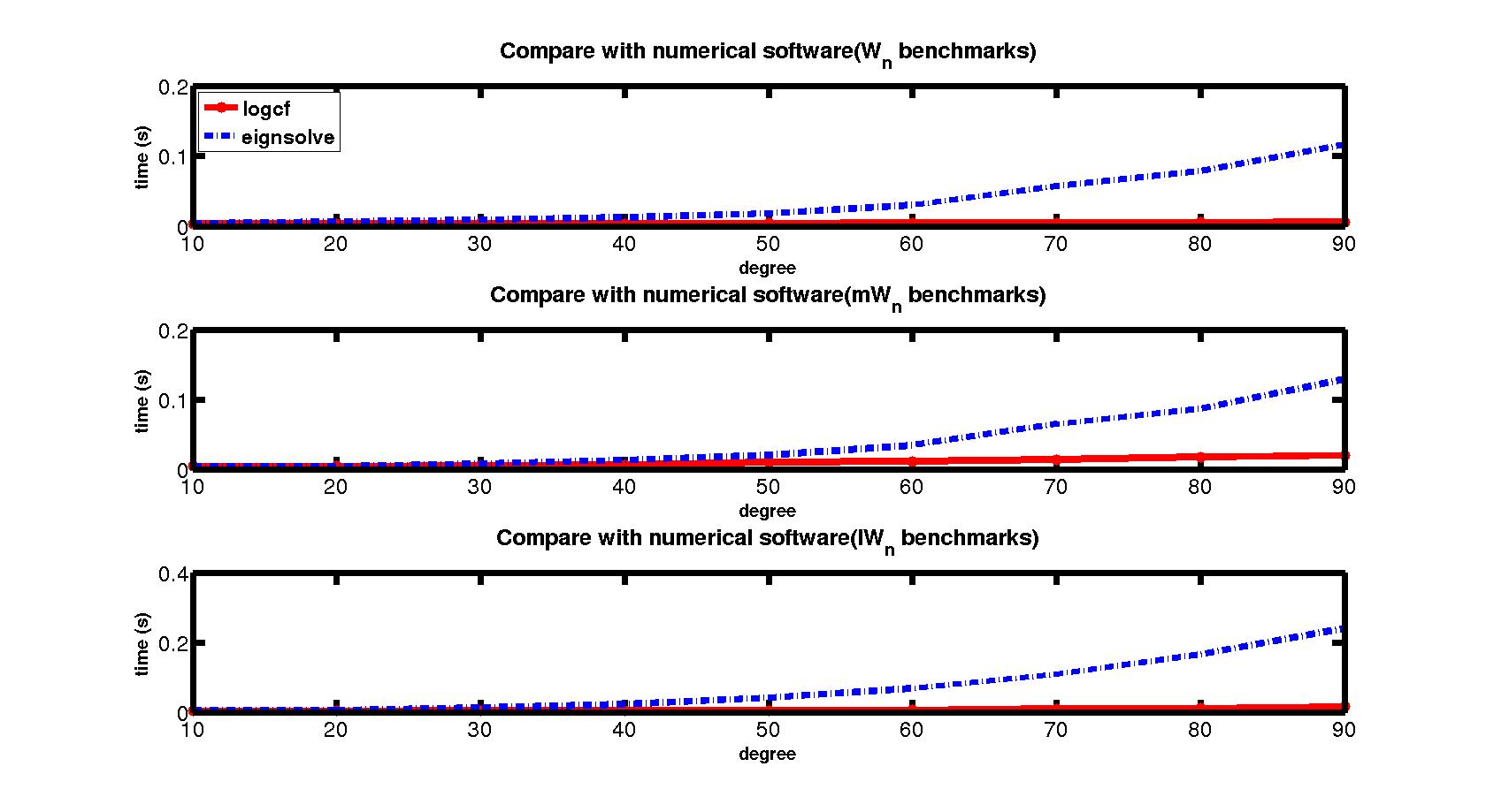
Figure 1: compare with numerical software eigensolve

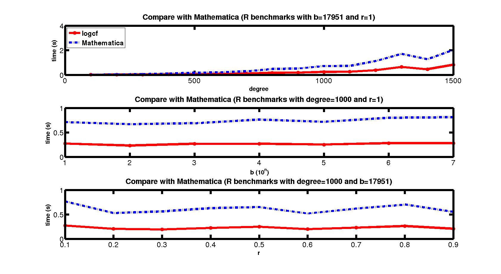
Figure 2: $R(n,b,r)$ benchmarks with differ setting

References

- [1] A. Akritas. An implementation of Vincent’s Theorem, Numer. Math. 36 53–62, 1980.
- [2] A. Akritas, and A. Strzeboński. A comparative study of two real root isolation methods, Nonlinear Analysis, Modelling and Control, 10 (4), 297–304, 2005.
- [3] A. Akritas, A. Strzeboński, and P. Vigklas. Implementations of a new theorem for computing bounds for positive roots of polynomials, Computing, 78, 355–367, 2006.
- [4] A. Akritas, A. Strzebonski, and P. Vigklas. Improving the performance of the continued fractions method using new bounds of positive roots. Nonlinear Analysis, 13(3):265–279, 2008.
- [5] G. Collins, A. Akritas. Polynomial real roots isolation using Descartes’ rule of signs. In: SYMSAC, 272–275, 1976.
- [6] A. Eigenwillig. Real root isolation for exact and approximate polynomials using Descartes’ rule of signs. Ph.D. Thesis, Saarland University, 2008.
- [7] A. Eigenwillig, L. Kettner, W. Krandick, K. Mehlhorn, S. Schmitt, N. Wolpert. A Descartes Algorithm for Polynomials with Bit-Stream Coefficients. In: CASC 2005, LNCS, 3718, 138–149, 2005.
- [8] S. Fortune. An iterated eigenvalue algorithm for approximating roots of univariate polynomials. J. Symb. Comput. 33(5), 627–646, 2002.
- [9] J. Gerhard. Modular algorithms in symbolic summation and symbolic integration. In: LNCS, 3218. Springer, 2004.
- [10] G.-M. Greuel, S. Laplagne, G. Pfister. normal.lib. A Singular 3-1-3 library for computing the normalization of affine rings, 2011.
- [11] M. Hemmer, E.P. Tsigaridas,Z. Zafeirakopoulos, I.Z. Emiris, M.I. Karavelas, B. Mourrain. Experimental evaluation and cross-benchmarking of univariate real solvers. In: SNC2009, 45–54, 2009.
- [12] H. Hong. Bounds for absolute positiveness of multivariate polynomials, J. symb. Comput. 25 (5), 571–585, 1998.
- [13] J. R. Johnson, W. Krandick, K. Lynch, D. Richardson, and A. Ruslanov. High-performance implementations of the Descartes method. In: Proc. ISSAC, 154–161, 2006.
- [14] J. R. Johnson, W. Krandick, and A. D. Ruslanov. Architecture-aware classical Taylor shift by 1. In: Proc. ISSAC, 200–207, 2005.
- [15] R. Klatte, U. Kulisch, C. Lawo, M. Rauch, A. Wiethoff. C-XSC: A C++ Class Library for Extended Scientific Computing, Springer, Berlin, 1993.
- [16] K. Mehlhorn and M. Sagraloff. A deterministic algorithm for isolating real roots of a real polynomial. J. Symb. Comput., 46:70–90, 2011.
- [17] B. Mourrain and J. P. Pavone. Subdivision methods for solving polynomial equations, J. Symb. Comput., 44, no. 3, 292–306, 2009.
- [18] F. Rouillier and P. Zimmermann. Efficient isolation of polynomials’ real roots. Comput. Math. Appl., 162:33–50, 2004.
- [19] S.M. Rump. INTLAB: INTerval LABoratory, in T. Csendes (ed.), Developments in Reliable Computing, Kluwer, 1999.
- [20] V. Sharma. Complexity of real root isolation using continued fractions. Theor. Comput. Sci.,409(2):292–310, 2008.
- [21] D. Ştefănescu. New bounds for the positive roots of polynomials, J. Universal Comput. Sci. 11 (12) 2132–2141, 2005.
- [22] E. P. Tsigaridas and I. Z. Emiris. On the complexity of real root isolation using continued fractions. Theor. Comput. Sci., 392(1-3):158–173, 2008.
- [23] B. Xia and T. Zhang. Real solution isolation using interval arithmetic.Comput. Math. Appl., 52:853–860, 2006.
- [24] T. Zhang and B. Xia. A new method for real root isolation of univariate polynomials. Mathematics in Computer Science, 1:305–320, 2007.