Funding Liquidity, Debt Tenor Structure,
and Creditor’s Belief: An Exogenous
Dynamic Debt Run Model

Abstract

We propose a unified structural credit risk model incorporating both insolvency and illiquidity risks, in order to investigate how a firm’s default probability depends on the liquidity risk associated with its financing structure. We assume the firm finances its risky assets by mainly issuing short- and long-term debt. Short-term debt can have either a discrete or a more realistic staggered tenor structure. At rollover dates of short-term debt, creditors face a dynamic coordination problem. We show that a unique threshold strategy (i.e., a debt run barrier) exists for short-term creditors to decide when to withdraw their funding, and this strategy is closely related to the solution of a non-standard optimal stopping time problem with control constraints. We decompose the total credit risk into an insolvency component and an illiquidity component based on such an endogenous debt run barrier together with an exogenous insolvency barrier.

Key words: Structural credit risk model, debt run, liquidity risk, first passage time, optimal stopping time

JEL Codes: G01, G20, G32, G33

1 Introduction

The recent financial crisis has dramatically shown that financial markets are not ideal. In particular, refinancing in periods of financial distress can be extremely costly or even impossible due to liquidity drying up in the market. It has been shown, for example by Adrian and Shin (2008, 2010) and Brunnermeier (2009), that the heavy use of short-term debt was a key contributing factor to the credit crunch of 2007/2008. Firms, however, often prefer short-term debt financing as it is cheaper than long-term debt. Moreover, as argued by He and Xiong (2012b), short-term debt can also be regarded as a disciplinary device for firms and can be used to mitigate adverse selection problems and to reduce the cost of auditing firms. Hence, several reasons support the use of short-term financing. However, most of the existing credit risk models do not take into account the rollover risk (or liquidity risk) inherent in short-term debt financing. It is the aim of this paper to provide a unified framework that incorporates rollover risk as well as insolvency risk. Within an extended structural credit risk model, our approach allows to investigate how a firm’s default probability depends on the rollover risk inherent in its particular financing structure.

Structural credit risk models were initiated by Merton (1974) and Black and Cox (1976). In these models default happens if the firm fundamental falls below some exogenous default barrier which often relates to the firm’s debt level. A huge part of the literature on structural credit risk modeling focuses on how to model such an exogenous default barrier, as in Longstaff and Schwartz (1995) and Briys and de Varenne (1997), among others. In the following we will call this exogenous default barrier the insolvency barrier. Given this exogenous insolvency barrier, in this paper we derive an endogenous threshold value below which short-term creditors decide to withdraw their funding, i.e., to run on the firm, and we will call this barrier the debt run barrier. The latter depends on not only the firm’s creditworthiness but also the creditors’ beliefs about the likelihood of a debt run in the remaining rollover periods. Determining this debt run barrier is the main problem of this paper. There is a third barrier, called the illiquidity barrier, which represents the critical value when the firm is unable to pay off its creditors in case of a debt run, and which is determined endogenously from the debt run barrier. In addition, we show that the debt run barrier always dominates the illiquidity barrier, which in turn dominates the insolvency barrier. This relationship among all three barriers not only helps to decompose the total credit risk into an insolvency component and an illiquidity component, but also illustrates the phenomenon that most firms have defaulted due to illiquidity rather than due to insolvency in the recent credit crunch.

Our first contribution is the provision of a rigorous formulation for a class of structural credit risk models that study debt runs. The classic debt/bank run model of Diamond and Dybvig (1983) features a static setting where all the depositors simultaneously decide whether or not to withdraw their demand deposits from a solvent but illiquid bank. Ericsson and Renault (2006) and Goldstein and Pauzner (2005) provide further extensions that are, however, still in the static setting. In this paper, we consider debt runs from a dynamic viewpoint. The debt run model introduced by Morris and Shin (2010) focuses on a two-period setting where short-term creditors face a binary decision in terms of global games at an interim time point. Liang et al. (2014) provide a structural credit risk model that also takes liquidity risk into account, as short-term creditors can decide at a finite number of decision dates whether to roll over or to withdraw their funding. They derive a debt/bank run barrier based on the comparison of binary strategies for a representative short-term creditor. Technically, the generalization from the two-period setting of Morris and Shin (2010) towards the multi-period setting of Liang et al. (2014) relies on the dynamic programming principle (DPP). In Liang et al. (2014) the DPP was only applied informally by comparing the expected returns for the two investment options of creditors at the rollover dates. In this paper, by introducing an appropriate value function for a representative short-term creditor, which describes the discounted expected return over the remaining rollover periods and which is calculated based on the DPP, we derive the unique threshold strategy, i.e., the debt run barrier. The representative creditor decides to withdraw her funding if the firm’s fundamental falls below this barrier at any decision date. In contrast to Liang et al. (2014), the corresponding dynamic programming equations presented in this paper are more generic and transparent, which in particular allows us to introduce flexible debt maturity structures into our model.

The second contribution of this paper is the imbedding of flexible debt tenor structures into such an extended structural credit risk model. In Liang et al. (2014) a discrete tenor structure is assumed such that the rollover dates of short-term debt are given by a sequence of deterministic numbers. This implies that all short-term debt expires and can be rolled over at the same time. The problem is therefore equivalent to a one-creditor problem. In reality, however, firms typically stagger the maturities for short-term debt to finance their long-term risky assets. Rollover risk is partially reduced in this way as at each maturity date only a fraction of total debt is due. Nevertheless, due to the maturity mismatch between the assets and the liabilities sides, the firm is still exposed to significant liquidity risk. Our model covers both the discrete tenor structure and the staggered tenor structure. The latter was first introduced by Leland (1994, 1998), and Leland and Toft (1996), with Hilberink and Rogers (2002) and Chen and Kou (2009) providing further technical details. The main idea is to assume a random duration of debt in order to reflect the maturity mismatch. Recently, He and Xiong (2012b) applied the staggered maturity structure to the debt run literature where debt maturities are modelled as arrival times of a Poisson process, whose intensity can then be interpreted as the inverse of average debt duration. In this paper, we utilize a more general and flexible Cox process to model the staggered tenor structure. The economic intuition of using the Cox maturity structure is that the average duration of the short-term debt which a firm issues should fluctuate and depend on some economic factors such as the firm fundamental or even the underlying systemic risk from the market.

The third contribution of this paper is that we use a reduced-form approach to model the impacts of other creditors’ rollover decisions on the representative short-term creditor’s rollover decision. In general, such impacts and the resulting equilibria are complicated as we need to consider not only the impact of other creditors’ current rollover decisions, but also the impact of their future decisions. In Morris and Shin (2010), they concentrate on the former impact, and resort to a reduced-form approach by modeling the representative short-term creditor’s belief on the proportion of creditors not rolling over their funding at each rollover date as a uniformly distributed random variable exogenously. In He and Xiong (2012b), they concentrate on the latter impact, and assume at each small time interval, there is only a small proportion of creditors whose contracts expire and need to be rolled over. In this paper, we try to include both impacts. The former impact is modeled in a similar way to Morris and Shin (2010) and Liang et al. (2014) by assuming the representative creditor’s belief exogenously. However, we take a more general model in the sense that the representative creditor’s belief is a general random variable, and we also compare the results with different assumptions on the distribution of such a random variable. The latter impact is included by considering the dynamic programming equation of the representative creditor, which is in the same spirit as He and Xiong (2012b).

Finally, our fourth contribution is to answer the question whether the representative short-term creditor’s rollover decision is indeed optimal. This question also arises in the existing dynamic debt run models such as those in Morris and Shin (2010), He and Xiong (2012b), and Liang et al. (2014), but has so far not been answered. In both the discrete and the staggered tenor structures, we show that the decision problem of the representative short-term creditor is equivalent to a non-standard optimal stopping time problem with control constraints. At each rollover date the representative creditor faces the risk that the firm may fail due to a debt run based on her belief. If the firm survives, the creditor can then decide whether to withdraw her funding (stop) or to roll over her contract (continue). If the firm fails due to other creditors’ runs, the representative creditor is then forced to stop and faces the recovery risk from bankruptcy. Therefore, the decision time for the representative creditor must exclude the default time due to debt runs. For the case of the staggered tenor structure, since the maturity dates are the arrival times of a Cox process, the representative creditor is only allowed to stop (i.e., to withdraw her funding) at a sequence of Cox arrival times rather than at any stopping time. In the literature, such kind of optimal stopping at Poisson-type arrival times has been used to solve the standard optimal stopping time problem by Krylov (2008) as the so-called randomized stopping time technique.

The paper is organized as follows. Section 2 describes the assumptions on the firm’s capital structure and explains the rollover decision of a representative short-term creditor in the benchmark model. We also present the rigorous formulation of the rollover decision problem in terms of dynamic programming equations. In section 3 we use the creditor’s value function derived in the dynamic programming equations to determine the short-term creditor’s debt run barrier as well as the firm’s illiquidity barrier in case of both the discrete and the staggered debt structures. We reformulate the creditor’s decision problem in terms of the associated optimal stochastic control problem in section 4. Section 5 discusses the related literature and concludes.

2 Benchmark Debt Run Model

In this section, we propose a debt run model that incorporates rollover risk into the structural credit risk framework.

2.1 Capital Structure of a Firm

Consider a market defined over a complete probability space $(\Omega,\mathcal{F},\mathbf{P})$, which supports a standard Brownian motion $(W_{t})_{t\geq 0}$ with its natural filtration $\{\mathcal{F}_{t}\}$ after augmentation. The market interest rate $r$ is assumed to be constant. In this market, consider a firm whose fundamental value of assets follows

$$\frac{dV_{t}}{V_{t}}=r_{V}dt+\sigma dW_{t},$$

with constant volatility $\sigma>0$. The constant $r_{V}$ denotes the expected return on the firm’s risky assets. We assume that the firm fundamental is publicly observable.

The firm finances its asset holdings in the duration $[0,T]$ by issuing short-term debt, such as asset-backed commercial papers and overnight repos, long-term debt such as corporate bonds, and equities and others. At initiation time $T_{0}=0$ an amount $L_{0}$ is borrowed long-term at rate $r_{L}$ until fixed maturity $T>0$. Moreover, an amount $S_{0}$ is borrowed short-term at rate $r_{S}$ until maturity $T_{1}$. When short-term debt matures it can be successively rolled over until the next rollover date. This produces a sequence of maturity dates (or rollover dates) $0=T_{0}<T_{1}<T_{2}\cdots<T_{\infty}=\infty$ for short-term debt. For the moment, we do not impose any structural conditions on the short-term debt maturities $\{T_{n}\}_{n\geq 1}$. They could be either deterministic or random.

If there is no default, the value of short-term debt follows

$$dS_{t}=r_{S}S_{t}dt,$$

and the value of long-term debt follows

$$dL_{t}=r_{L}L_{t}dt.$$

The ratio of long-term debt over short-term debt $L_{t}/S_{t}$ is denoted by $l_{t}$ and follows

$$dl_{t}=(r_{L}-r_{S})l_{t}dt.$$

Moreover, we introduce a process $X_{t}$ as the ratio of the firm’s asset value over the short-term debt value $X_{t}=V_{t}/S_{t}$. Hence, $X_{t}$ follows

$$\frac{dX_{t}}{X_{t}}=(r_{V}-r_{S})dt+\sigma dW_{t}.$$

Short-term creditors have the opportunity to withdraw their funding at the rollover dates. When the firm is under financial distress or when an outside investment opportunity is more attractive they will make use of this option. Long-term creditors, however, are locked in once they lend money to the firm. They are exposed to a higher risk, and therefore, should be rewarded with a higher interest rate. Moreover, since creditors are exposed to the firm’s default risk, a risk premium should be paid on top of the market interest rate. We have the following assumption on different interest rates.

Assumption 2.1

The long-term interest rate $r_{L}$ is strictly greater than the short-term interest rate $r_{S}$, while the latter is strictly greater than the market interest rate $r$, i.e., we assume $r_{L}>r_{S}>r$.

2.2 The Rollover Decision of a Representative Short-Term Creditor

Short-term creditors choose whether to renew their maturing contracts, that is, they need to decide whether to roll over or to withdraw their funding (i.e., to run) at the maturity times. Hence, they face a dynamic coordination problem.

Consider the decision problem of a representative short-term creditor. The first key factor to determine the representative short-term creditor’s rollover decision is the insolvency risk stemming from the deterioration of the firm fundamental. To include this factor, we follow the classic first-passage-time framework (see for example Black and Cox (1976)) by assuming an exogenously given insolvency barrier

$$D_{t}^{Ins}=S_{t}\beta(l_{t}),$$

where $\beta:(0,\infty)\rightarrow(0,\infty)$ is a safety covenant function of the ratio $l_{t}=L_{t}/S_{t}$. As long as the asset value $V_{t}$ at any time $t$ is greater than or equal to the total value of debt $S_{t}+L_{t}$, the firm can be considered solvent. Hence, it is natural to assume that

$$\beta(l_{t})\leq(1+l_{t})$$ (2.1)

such that

$$D_{t}^{Ins}=S_{t}\beta(l_{t})\leq S_{t}(1+l_{t})=S_{t}+L_{t}.$$

The bankruptcy time due to insolvency is then given by the following first-passage-time

$$\tau^{Ins}=\inf\{t\geq 0:V_{t}\leq D_{t}^{Ins}\}=\inf\{t\geq 0:X_{t}\leq\beta(l_{t})\}.$$

To coordinate with other creditors, the representative creditor needs to take other creditors’ rollover decisions into account, and makes her own decision based on whether the firm will survive debt runs or not at each rollover date $T_{n}$. Assume that the creditor believes that the proportion of short-term creditors not rolling over their funding at each rollover date $T_{n}$ is a random variable $\xi$ supported on $[0,1]$ with its conditional density $f(\cdot|X_{T_{n}})$ given $X_{T_{n}}$.

The firm will survive debt runs if it can raise enough funding to pay off its creditors who run on the firm and still keep solvent. In case of a debt run the firm has to issue collateralized debt by pledging its assets as collateral to raise the liquidity. The actual value of the collateral does not matter. It is the maximum value of the collateral that determines whether the firm is still liquid or not. The maximum collateral value of the assets is expressed in terms of the fire-sale price $\psi V_{T_{n}}$ with the fire-sale rate $\psi\in(0,1)$. If $\psi V_{T_{n}}\geq\xi S_{T_{n}}$, the firm is able to pay off its creditors who run on the firm, so a potential debt run at time $T_{n}$ would not lead to a default. Hence, the second key factor determining the creditor’s rollover decision is her belief about the probability that the firm survives the debt run at the rollover date $T_{n}$, which equals

$$\theta(X_{T_{n}}) =\mathbf{P}\left(\psi V_{T_{n}}\geq\xi S_{T_{n}}|X_{T_{n}}\right)$$

$$=\mathbf{P}\left(\psi X_{T_{n}}\geq\xi|X_{T_{n}}\right)$$

$$=\mathbf{P}\left(0\leq\xi\leq\min\{1,\psi X_{T_{n}}\}|X_{T_{n}}\right)=\int_{0}^{\min\{1,\psi X_{T_{n}}\}}f(x|X_{T_{n}})dx$$ (2.2)

conditional on the firm being solvent at $T_{n}$, i.e. on the event $\{V_{T_{n}}\geq D^{Ins}_{T_{n}}\}$. In both Morris and Shin (2010) and Liang et al. (2014), the random variable $\xi$ is simply assumed to be uniformly distributed on $[0,1]$, so that $f(\cdot|X_{T_{n}})=1$ and

$$\theta(X_{T_{n}})=\min\{1,\psi X_{T_{n}}\}.$$

This assumption is justified by global games theory as it has been shown in Morris and Shin (2003) that this is a limiting case of the situation with unobservable firm fundamental when the variance of the noise term tends to zero. In section 3.2, we will show that the uniform distribution assumption is relatively robust by comparing it to a family of truncated normal distributions with the same mean but different variances.

The third key factor for the representative short-term creditor’s rollover decision is the recovery rate when the firm defaults either due to debt runs or due to insolvency. If the firm defaults at some time $t\in[0,T]$, the firm is exposed to certain bankruptcy costs. Suppose these are proportional to the firm fundamental value, and for $\alpha\in(0,1)$, $\alpha V_{t}$ is the firm value after having paid the bankruptcy costs. Then, the value $\alpha V_{t}$ will be divided among all the creditors, so the representative short-term creditor obtains the proportion of her funding and she gets at most her debt value back. Thus, we define the recovery rate as

$$R_{t}=\min\left\{1,\frac{\alpha V_{t}}{S_{t}+L_{t}}\right\}=\min\left\{1,\frac{\alpha X_{t}}{1+l_{t}}\right\}.$$ (2.3)

Note that in case of a default due to a debt run, it can happen that the asset value is larger than $S_{t}+L_{t}$. Therefore, we have to cut off the recovery rate by $1.$ However, if the firm defaults due to insolvency at the first-passage-time $\tau^{Ins}$, the asset value by definition equals the insolvency barrier $D^{Ins}_{\tau^{Ins}}$. In this case the recovery rate equals

$$R_{\tau^{Ins}}=\frac{\alpha D_{\tau^{Ins}}^{Ins}}{S_{\tau^{Ins}}+L_{\tau^{Ins}}}=\frac{\alpha\beta(l_{\tau^{Ins}})}{1+l_{\tau^{Ins}}}$$

which is less than 1 by condition (2.1).

We assume that rollover decisions are solely determined by the aforementioned factors, which we summarize as follows.

Assumption 2.2

The following three factors determine the rollover decision of a representative short-term creditor.

• Insolvency risk is reflected by the first-passage-time $\tau^{Ins}$ when the firm’s asset value falls below the insolvency barrier $D_{t}^{Ins}$.

• Rollover risk is reflected by the representative short-term creditor’s belief on the probability $\theta(X_{T_{n}})$ that the firm survives the debt run at the rollover date $T_{n}$.

• Recovery risk is reflected by the fraction $R_{t}$ of funding that the representative short-term creditor obtains in case of a default at time $t$.

We further impose the following condition on the safety covenant function for technical convenience.

Assumption 2.3

The safety covenant function $\beta(l_{t})$ in the definition of the insolvency barrier $D_{t}^{Ins}$ has the linear form $\beta(l_{t})=\beta l_{t}$ for some positive constant $\beta\leq(1/l_{t}+1)$.

2.3 Dynamic Programming Equations

In this section we derive dynamic programming equations for the short-term creditor’s rollover decision problem. We consider a representative short-term creditor who invests an amount normalized to 1 monetary unit at time $t\in[0,T]$. Her discounted expected return over the remaining time period $[t,T]$ is described by the value function $U(t,x)$ given the current ratio $X_{t}=x$ of asset value over short-term debt value, and she discounts at the market rate $r$. To investigate the creditor’s value function we go backwards in time starting with her last rollover date prior to terminal time $T$. Suppose that her $N^{\rm th}$ rollover date is the closest one prior to the maturity $T$ of long-term debt, that is, $T_{N}<T$ and $T_{N+1}\geq T$. Figure 1 illustrates the maturities of the short- and long-term debt. If the maturities are random (as in section 3.2), then what we do in the following is to condition on one realization of $\{T_{n}(\omega)\}_{n\geq 1}$ so that $T_{N}(\omega)<T\leq T_{N+1}(\omega)$. By abuse of notation, we continue to write $T_{n}$ for $T_{n}(\omega)$ in such a case.

Figure 1: Maturities of Short- and Long-Term Debt

$\drawline(0,50)(330,50)\drawline(10,47)(10,53)\drawline(40,47)(40,53)\drawline(110,47)(110,53)\drawline(220,47)(220,53)\drawline(250,47)(250,53)\drawline(290,47)(290,53)\tagcurve(37,53,25,70,13,53)\tagcurve(13,53,25,70,37,53)\drawline(37,53)(31,53)\drawline(37,53)(38,62)\tagcurve(105,55,75,75,45,55)\tagcurve(45,55,75,75,105,55)\drawline(105,55)(98,53)\drawline(105,55)(103,62)\tagcurve(223,53,255,70,287,53)\tagcurve(287,53,255,70,223,53)\drawline(287,53)(280,53)\drawline(287,53)(287,62){\tagcurve(15,35,120,10,245,35)\tagcurve(245,35,120,10,15,35)\drawline(245,35)(238,37)\drawline(245,35)(243,30)}\drawline(325,45)(330,50)\drawline(325,55)(330,50)\put(10.0,40.0){$T_{0}$}\put(25.0,75.0){$r_{S}$}\put(40.0,40.0){$T_{1}$}\put(75.0,78.0){$r_{S}$}\put(110.0,40.0){$T_{2}$}\put(150.0,40.0){$\ldots$}\put(253.0,75.0){$r_{S}$}\put(120.0,1.0){{$r_{L}$}}\put(220.0,40.0){$T_{N}$}\put(250.0,40.0){{$T$}}\put(290.0,40.0){$T_{N+1}$}$

At the terminal time $T$, the representative short-term creditor faces the insolvency risk that the firm may not pay back her funding, and her value function at the terminal time is

$$U(T,x)=R_{T}=\min\left\{1,\frac{x}{1+l_{T}}\right\},$$ (2.4)

which represents the insolvency risk stemming from the final workout of the firm fundamental as in Merton (1974).

During the last time period $(T_{N},T)$, all of the creditors are locked in, so there is no rollover risk, and the representative short-term creditor only faces the insolvency risk with the associated recovery risk. Her value function for $t\in(T_{N},T)$ is

$$U(t,x)= \ \mathbf{E}_{t}^{x}\left\{\mathbf{1}_{\{t\leq\tau^{Ins}<T\}}e^{-r(\tau^{Ins}-t)}\cdot e^{r_{S}(\tau^{Ins}-t)}R_{\tau^{Ins}}\right.$$

$$+\left.\mathbf{1}_{\{\tau^{Ins}\geq T\}}e^{-r(T-t)}\cdot e^{r_{S}(T-t)}U(T,X_{T})\right\},$$ (2.5)

where the first term in the bracket captures the insolvency risk from the firm fundamental falling below the insolvency barrier $D_{t}^{Ins}$ during the time period $(t,T)$, and the second term captures the insolvency risk from the final workout of the firm’s risky project at time $T$. Hence, (2.3) represents the insolvency risk due to the deterioration of the firm fundamental as in Black and Cox (1976).

To determine the value function at $t=T_{N}$ we take a closer look at the rollover decision problem. At the rollover date $T_{N}$, if the firm survives a debt run, the representative short-term creditor will compare the expected return from rolling over her funding with the expected market return, and will choose whatever results in a higher return for her. If the firm defaults due to a debt run, she will receive the recovery value $R_{T_{N}}$ in any case, regardless of whether she decides to roll over her funding or not. Hence, the creditor can only make her rollover decision conditional on the firm surviving the current debt run. Therefore, the value function given in equation (2.3) also describes her discounted expected return at time $t=T_{N}$ for the remaining time period $(T_{N},T)$.

In general, during the time period $[T_{n},T_{n+1})$ for $n=0,1,\ldots,N-1$, the representative short-term creditor is exposed not only to the insolvency risk arising from the deterioration of the firm fundamental in the period $[T_{n},T_{n+1})$ but also to the rollover risk caused by other creditors’ rollover decisions at time $T_{n+1}$. Table 1 summarizes her payoff at maturity $T_{n+1}$.

Table 1: Representative creditor’s aggregate payoff from $T_{n}$ to $T_{n+1}$

Decision	Solvency in $[T_{n},T_{n+1}]$,	Solvency in $[T_{n},T_{n+1}]$,	Insolvency in $[T_{n},T_{n+1}]$.
at $T_{n+1}$	no default due to run at $T_{n+1}$.	default due to run at $T_{n+1}$.
Run	$e^{r_{S}(T_{n+1}-T_{n})}\cdot 1$	$e^{r_{S}(T_{n+1}-T_{n})}\cdot R_{T_{n+1}}$	$e^{r_{S}(\tau^{Ins}-T_{n})}R_{\tau^{Ins}}$
Rollover	$e^{r_{S}(T_{n+1}-T_{n})}\cdot U(T_{n+1},X_{T_{n+1}})$	$e^{r_{S}(T_{n+1}-T_{n})}\cdot R_{T_{n+1}}$	$e^{r_{S}(\tau^{Ins}-T_{n})}R_{\tau^{Ins}}$

At maturity $T_{n+1}$ if there is no default, the representative short-term creditor either withdraws her funding to get $e^{r_{S}(T_{n+1}-T_{n})}\cdot 1$ or renews her contract to receive $e^{r_{S}(T_{n+1}-T_{n})}\cdot U(T_{n+1},X_{T_{n+1}})$. If the firm defaults due to a debt run at time $T_{n+1}$, the creditor just gets the fraction $R_{T_{n+1}}$ of her funding $e^{r_{S}(T_{n+1}-T_{n})}$ back. Since the creditor believes that the firm survives a debt run at time $T_{n+1}$ with probability $\theta(X_{T_{n+1}})$, her discounted expected return at time $t\in[T_{n},T_{n+1})$ can be described by the following value function

$$U(t,x)= \ \mathbf{E}_{t}^{x}\left\{\mathbf{1}_{\{t\leq\tau^{Ins}<T_{n+1}\}}e^{(r_{S}-r)(\tau^{Ins}-t)}R_{\tau^{Ins}}+\mathbf{1}_{\{\tau^{Ins}\geq T_{n+1}\}}e^{(r_{S}-r)(T_{n+1}-t)}\cdot\right.$$

$$\hskip 28.45274pt\left.\cdot\left[\theta(X_{T_{n+1}})\max\left\{1,U(T_{n+1},X_{T_{n+1}})\right\}+(1-\theta(X_{T_{n+1}}))R_{T_{n+1}}\right]\right\}.$$ (2.6)

The first term on the right hand side captures the insolvency risk within the time period $[t,T_{n+1})$, whereas the second term captures the rollover risk at time $T_{n+1}$ as well as the insolvency and rollover risks in $[T_{n+1},T]$. Therefore, the first term in the second line of (2.3) represents the future rollover risk (and insolvency risk) as in He and Xiong (2012b), and the second term in the second line of (2.3) represents the current rollover risk as in Morris and Shin (2010). Note that if the maturities are random, then both (2.3) and (2.3) are understood as conditioning on one realization of $\{T_{n}(\omega)\}_{n\geq 1}$ so that $T_{N}<T\leq T_{N+1}$.

The dynamic programming equations (2.3) and (2.3) for the value function $U(t,x)$ are the drivers to determine the debt run barrier in our model, which will be discussed later. By the Feynman-Kac formula, we have the following partial differential equation (PDE) representation for the value function $U(t,x)$.

Proposition 2.1

Suppose Assumptions 2.1, 2.2, and 2.3 are satisfied. For $n=0,1,\ldots,N-1$, let $W_{n}(t,x)$ be the unique solution to the following PDE Dirichlet problem on $[T_{n},T_{n+1}]\times[\beta l_{t},\infty)$

$$\left\{\begin{array}[]{l}\frac{\partial W_{n}}{\partial t}+\mathcal{L}W_{n}+(r_{S}-r)W_{n}=0\\[11.38092pt] W_{n}(t,\beta l_{t})=\alpha\beta l_{t}/(1+l_{t})\\[11.38092pt] W_{n}(T_{n+1},x)=\theta(x)\max\left\{1,W_{n+1}(T_{n+1},x)\right\}+(1-\theta(x))\alpha x/(1+l_{T_{n+1}}).\end{array}\right.$$ (2.7)

For $n=N$, let $W_{N}(t,x)$ be the unique solution to the following Dirichlet problem on $[T_{N},T]\times[\beta l_{t},\infty)$

$$\left\{\begin{array}[]{l}\frac{\partial W_{N}}{\partial t}+\mathcal{L}W_{N}+(r_{S}-r)W_{N}=0\\[11.38092pt] W_{N}(t,\beta l_{t})=\alpha\beta l_{t}/(1+l_{t})\\[11.38092pt] W_{N}(T,x)=\min\left\{1,x/(1+l_{T})\right\},\end{array}\right.$$ (2.8)

where $\mathcal{L}$ is the infinitesimal generator for the ratio process $X$ given by

$$\mathcal{L}=\frac{1}{2}\sigma^{2}x^{2}\frac{\partial^{2}}{\partial x^{2}}+(r_{V}-r_{S})x\frac{\partial}{\partial x}.$$

Then the value function $U(t,x)$ is given by concatenating $W_{n}(t,x)$ together

$$U(t,x)=W_{n}(t,x)\ \ \text{for}\ \ t\in[T_{n},T_{n+1}).$$

Based on the Green’s function technique, we further have the following analytical representation for the value function $U(t,\bar{x})$ where $\bar{x}=x/(\beta l_{t})$.

Proposition 2.2

(Green’s Representation) For $n=0,1,\ldots,N$, denote $P_{n}$ and $\Phi_{n}$ respectively as the boundary condition and the terminal condition of the corresponding PDE for the value function $U(t,\bar{x})$ on $[T_{n},T_{n+1})$, where $T_{N+1}:=T$ for convenience. Then

$$U(t,\bar{x})=\int_{1}^{\infty}P_{n}(\xi)\mathbb{G}(t,\bar{x};T_{n+1},\xi)d\xi+\frac{1}{2}\sigma^{2}\int_{t}^{T_{n+1}}\Phi_{n}(\eta)\frac{\partial}{\partial\xi}\left.\left\{\xi^{2}\mathbb{G}(t,\bar{x};\eta,\xi)\right\}\right|_{\xi=1}d\eta$$ (2.9)

on $[T_{n},T_{n+1})$, where $\mathbb{G}(t,\bar{x};\eta,\xi)$ is the Green’s function for the operator $\mathcal{L}^{v}$ defined as

$$\mathcal{L}^{v}=\frac{\partial}{\partial t}+\frac{1}{2}\sigma^{2}\bar{x}^{2}\frac{\partial^{2}}{\partial\bar{x}^{2}}+(r_{V}-r_{L})\bar{x}\frac{\partial}{\partial\bar{x}}+(r_{S}-r)$$

on the domain $[T_{n},T_{n+1}]\times[1,\infty)$ given by

$$\mathbb{G}(t,\bar{x};T_{n+1},\xi)= \ \frac{e^{(r_{S}-r)(T_{n+1}-t)}}{\xi\sigma\sqrt{2\pi(T_{n+1}-t)}}\exp\left\{-\frac{\left[\log\frac{\bar{x}}{\xi}+(r_{V}-r_{L}-\frac{1}{2}\sigma^{2})(T_{n+1}-t)\right]^{2}}{2\sigma^{2}(T_{n+1}-t)}\right\}$$

$$\times\left[1-\exp\left\{\frac{2\log\frac{1}{\xi}\log\bar{x}}{\sigma^{2}(T_{n+1}-t)}\right\}\right].$$

Proof. See Appendix A.1.   

3 Threshold Strategies of Debt Run Model

In this section, we use the dynamic programming equations (2.3) and (2.3) to determine the debt run barrier as well as the illiquidity barrier for the representative short-term creditor. Our main objective is to show the monotonic relationship among the debt run barrier, the illiquidity barrier, and the exogenously given insolvency barrier.

3.1 Discrete Tenor Structure: Revisit of Liang et al. (2014)

In this subsection, we extend the main results in Liang et al. (2014) to our general setup. Liang et al. (2014) show that there exists a threshold, called the debt run barrier such that the representative short-term creditor will withdraw her funding whenever the firm fundamental falls below this barrier at a rollover date. The debt run barrier is only a finite sequence of numbers, since the creditor only has a finite number of rollover dates to decide whether to run or not. In our general setting we define the debt run barrier $D_{T_{n}}^{Run}$ for any $n=0,1,\ldots,N$ as the critical asset value such that the representative short-term creditor is indifferent in terms of running or rolling over her debt, i.e., it is defined via the unique value $x_{T_{n}}^{*}$ such that $1=U(T_{n},x^{*}_{T_{n}})$ in the maximum term in dynamic programming equation (2.3). The debt run barrier $D_{T_{n}}^{Run}$ is then determined by

$$D_{T_{n}}^{Run}=x^{*}_{T_{n}}S_{T_{n}}=x^{*}_{T_{n}}S_{0}e^{r_{S}T_{n}},\ \ \ \text{for}\ n=0,1,\ldots,N.$$

Since such a debt run barrier is determined by the representative short-term creditor, it is actually the debt run barrier for all of the short-term creditors, who will then run on the firm if $V_{T_{n}}\leq D_{T_{n}}^{Run}$. Although the representative creditor (so every short-term creditor) holds the belief that $\xi$ proportion of them will run on the firm at each date $T_{n}$, they will actually run at the same time based on such a debt run barrier strategy. In fact, such kind of debt run barrier strategy also appears in dynamic debt run models such as Morris and Shin (2010), He and Xiong (2012b) and Liang et al. (2014).

In the following, we show that such a debt run barrier always dominates the insolvency barrier. Note that the value function $U(t,x)$ is obviously increasing with respect to $x$, and when the firm goes bankrupt due to insolvency at a rollover date $T_{n}=\tau^{Ins}$, the value function is

$$U(T_{n},\beta l_{T_{n}})=R_{T_{n}}=\alpha\beta l_{T_{n}}/(1+l_{T_{n}}).$$

Due to Assumption 2.3 we have $\beta\leq(1/l_{T_{n}}+1)$ so that $U(T_{n},\beta l_{T_{n}})\leq 1=U(T_{n},x^{*}_{T_{n}})$. Hence we have $\beta l_{T_{n}}\leq x^{*}_{T_{n}}$. This means the insolvency barrier $D_{t}^{Ins}$ at any rollover date $t=T_{n}$ is dominated by the debt run barrier, i.e., $D_{T_{n}}^{Ins}\leq D_{T_{n}}^{Run}$ for $n=0,1,\ldots,N.$ Note that this dominance always holds in Liang et al. (2014), since the recovery rate $R_{t}$ is assumed to be zero therein.

A debt run does not necessarily trigger a default, for example in the case where the firm can raise enough funding to pay off its maturing short-term debt. The firm will survive the debt run at the rollover date $T_{n}$, if $\psi V_{T_{n}}\geq S_{T_{n}}$ conditional on $V_{T_{n}}\geq D_{T_{n}}^{Ins}$. Motivated by this observation we introduce a third barrier, which we call an illiquidity barrier $D^{Ill}$, and which is defined as follows

$$D_{T_{n}}^{Ill}=\min\left\{D_{T_{n}}^{Run},\max\{S_{T_{n}}/\psi,D^{Ins}_{T_{n}}\}\right\},\ \ \ \text{for}\ n=0,1,\ldots,N.$$ (3.1)

Hence, an illiquidity default only occurs if there is a debt run and the firm is not able to raise enough funds to pay off its maturing short-term debt or not able to remain solvent at the debt run.

In the following, we show that the insolvency barrier $D_{t}^{Ins}$ at $t=T_{n}$ is also dominated by the illiquidity barrier, i.e., $D_{T_{n}}^{Ins}\leq D_{T_{n}}^{Ill}$ for $n=0,1,\ldots,N.$ Indeed, we always have

$$D_{T_{n}}^{Ill}\geq\min\{D^{Run}_{T_{n}},D^{Ins}_{T_{n}}\}=D^{Ins}_{T_{n}}.$$

Theorem 3.1

Suppose that Assumptions 2.1, 2.2, and 2.3 are satisfied. Then at any maturity $T_{n}$, the debt run barrier is no less than the illiquidity barrier, while the latter is no less than the insolvency barrier, i.e.,

$$D_{T_{n}}^{Ins}\leq D_{T_{n}}^{Ill}\leq D_{T_{n}}^{Run}\ \ \ \text{for}\ n=0,1,\ldots,N.$$

Due to this relationship, the debt run barrier, the illiquidity barrier and the insolvency barrier determine four possible scenarios at each of the rollover dates $T_{n}$ which are illustrated in the flowchart in Figure 2.

[Insert Figure 2 here.]

Figure 3 shows different scenarios in our debt run model with the discrete tenor structure for three simulated asset value paths. Here we assume $\xi$ is uniformly distributed, and $N=4$ rollover dates at times $t=2,4,6,$ and $8$. The dotted line shows the debt run barrier, the dashed line the illiquidity barrier, and the solid line the insolvency barrier. Note that in this discrete setting, the debt run barrier and the illiquidity barrier are not continuous functions. They consist only of the marked points. The black asset value path falls below the insolvency barrier shortly before time $t=4.$ At the rollover date $t=2$ prior to this time, the asset value is larger than the debt run barrier. Hence, in this simulation the firm will default shortly before time $t=4$ due to insolvency. The dark black path falls below the illiquidity barrier at the third rollover date at time $t=6$,and before time $t=6$ it always stays above the insolvency barrier. Thus, in this simulation the firm defaults due to illiquidity at time $t=6$. Finally, the grey path shows a scenario where a debt run occurs at the last rollover date $t=8$. At that time, however, the asset value is still larger than the illiquidity barrier, meaning that the firm is able to raise enough funds to pay off its short-term creditors. Hence, the firm survives the debt run.

[Insert Figure 3 here.]

3.2 Staggered Tenor Structure

In Liang et al. (2014) it is assumed that short-term debt rollover dates are given by a deterministic sequence of numbers and that they are the same for all short-term creditors. This assumption is rather restrictive. The firm is highly exposed to rollover risk in such a setting where all short-term funding expires at the same date. In practice, however, firms tend to spread out their debt expirations across time to reduce their exposure to liquidity risk. In this section, we introduce a more flexible debt maturity structure. Among others, Leland (1994, 1998) and Leland and Toft (1996) introduced the so-called staggered maturity structure to capture this fact. The idea is to use the arrival times of a Poisson process to model the maturities of short-term debt. In other words, the duration of short-term debt $T_{1}-T_{0},T_{2}-T_{1},\ldots$ has an exponential distribution. While the random duration assumption appears different from the standard debt contract with a predetermined maturity, it captures the staggered debt maturity structure of a typical firm. For the application of such a Poisson maturity structure in the literature of debt runs, we refer to the recent work by He and Xiong (2012b).

The crucial parameter under the aforementioned Poisson maturity structure framework is the intensity $\lambda$. Its inverse $1/\lambda$ can be interpreted as the average duration of short-term debt. We consider a Cox maturity structure, meaning that the maturity of short-term debt follows a more general and flexible Cox process. Recall that a Cox process is a generalization of Poisson processes in which the intensity is allowed to be random but in such a way that if we condition on a particular realization $\lambda_{t}(\omega)$ of the intensity, the process becomes an inhomogeneous Poisson process with intensity $\lambda_{t}(\omega)$. The economic intuition of using the Cox maturity structure is that the average duration of the short-term debt that the firm issues should depend on some time-dependent economic factors such as the firm fundamental $V$, the ratio $X$ of the firm fundamental over the short-term debt, or even some underlying states of the economy. In the following we therefore assume that the average maturity is a function of the ratio process $X$.

We construct the short-term debt maturities $\{T_{n}\}_{n\geq 1}$ by so-called canonical construction. Let $\{E_{n}\}_{n\geq 1}$ be a sequence of independent identically distributed (i.i.d.) exponential random variables on some complete probability space $(\tilde{\Omega},\tilde{\mathcal{F}},\tilde{\mathbf{P}})$, and define the enlarged probability space by

$$\bar{\Omega}=\Omega\times\tilde{\Omega},\ \ \ \bar{\mathcal{G}}=\mathcal{F}\otimes\tilde{\mathcal{F}},\ \ \ \text{and}\ \ \mathbf{Q}=\mathbf{P}\otimes\tilde{\mathbf{P}}.$$

We assume the intensity has the form $\lambda_{t}=g(X_{t})$, where $g:(0,\infty)\rightarrow(0,\infty)$ is a smooth function with compact support. Then the maturities of short-term debt are constructed recursively as

$$T_{0}=0\quad\mbox{and}\quad T_{n}=\inf\left\{t\geq T_{n-1}:\int_{T_{n-1}}^{t}g(X_{s})ds\geq E_{n}\right\},\quad\mbox{for}\,n\geq 1.$$

We summarize the above construction in the following assumption.

Assumption 3.1

(Cox maturity structure) The maturities of the short-term debt $\{T_{n}\}_{n\geq 1}$ are the arrival times of a Cox process with intensity $g(X_{t})$.

Under the Cox maturity structure, we still employ the representative short-term creditor’s dynamic programming equations (2.3) and (2.3) to determine her value function $U(t,x)$. Letting the ratio process start from $X_{t}=x$ and the short-term debt maturities start from $T_{0}=t$, we synthesize the dynamic programming equations (2.3) and (2.3) into the following succinct form on the event $\{{T_{1}>t}\}$:

$$\ U(t,x)$$

$$= \ \mathbf{E}_{t}^{x}\left\{\mathbf{1}_{\{t\leq\tau^{Ins}<T\}}\left[\mathbf{1}_{\{t<T_{1}<\tau^{Ins}\}}e^{(r_{S}-r)(T_{1}-t)}\left[\theta(X_{T_{1}})\max\left\{1,U(T_{1},X_{T_{1}})\right\}+(1-\theta(X_{T_{1}}))R_{T_{1}}\right]\right.\right.$$

$$\ \ \ \ \ \ \ \ \ \ \ \ \ \ \ \ \ \ \ \ \ \ \ \ \left.+\mathbf{1}_{\{T_{1}\geq\tau^{Ins}\}}e^{(r_{S}-r)(\tau^{Ins}-t)}R_{\tau^{Ins}}\right]$$

$$+\mathbf{1}_{\{\tau^{Ins}\geq T\}}\left[\mathbf{1}_{\{t<T_{1}<T\}}e^{(r_{S}-r)(T_{1}-t)}\left[\theta(X_{T_{1}})\max\left\{1,U(T_{1},X_{T_{1}})\right\}+(1-\theta(X_{T_{1}}))R_{T_{1}}\right]\right.$$

$$\ \ \ \ \ \ \ \ \ \ \ \ \ \ \ \ \ \ \ \ \ \ \ \ \left.\left.+\mathbf{1}_{\{T_{1}\geq T\}}e^{(r_{S}-r)(T-t)}\min\left\{1,X_{T}/(1+l_{T})\right\}\right]\right\}.$$ (3.2)

By using the distribution of the first arrival time $T_{1}$, and applying the Feynman-Kac formula, we derive the following PDE representation for the value function $U(t,x)$ under the Cox maturity structure.

Proposition 3.2

Suppose that Assumptions 2.1, 2.2, 2.3 and 3.1 are satisfied. Then the value function $U(t,x)$ satisfies the following semi-linear PDE Dirichlet problem on $[0,T]\times[\beta l_{t},\infty)$:

$$\left\{\begin{array}[]{l}\frac{\partial U}{\partial t}+\mathcal{L}U+(r_{S}-r-g(x))U\\[11.38092pt] \ \ \ \ +g(x)[\theta(x)\max\{1,U\}+(1-\theta(x))\alpha x/(1+l_{t})]=0\\[11.38092pt] U(t,\beta l_{t})=\alpha\beta l_{t}/(1+l_{t})\\[11.38092pt] U(T,x)=\min\left\{1,x/(1+l_{T})\right\}.\end{array}\right.$$ (3.3)

Proof. See Appendix A.2.   

In Appendix B, we provide a numerical algorithm to approximate the solution of the above PDE (3.3). In the rest of this section, we show that PDE (3.3) implies a unique threshold for the representative short-term creditor, i.e., there exists a unique debt run barrier $D_{t}^{Run}$ such that she will run on the firm whenever both the firm’s asset value falls below such a barrier and her contract expires at some maturity $T_{n}$. Thus, the debt run time in our model is characterized endogenously by the following first-passage-time

$$\tau^{Run}=\inf\{T_{n}:X_{T_{n}}\leq x^{*}(T_{n})\}\wedge T,$$

where $x^{*}(t)$ is the threshold we shall derive in the remainder of this section. Recall that $X_{t}=V_{t}/S_{t}$ is the ratio of the firm fundamental over the short-term debt, so the debt run barrier $D_{t}^{Run}$ is given as

$$D_{t}^{Run}=x^{*}(t)S_{t}=x^{*}(t)S_{0}e^{r_{S}t}.$$

We derive a free-boundary problem to determine first the threshold $x^{*}(t)$ and secondly the debt run barrier $D_{t}^{Run}$ based on the semi-linear PDE (3.3).

• If $x>x^{*}(t)$, the representative short-term creditor will keep lending her money to the firm because either the debt is not due yet or if the debt is due she decides to roll over her funding. Her value function $U(t,x)>1$, and (3.3) reduces to

  $$\frac{\partial U}{\partial t}+\mathcal{L}U+(r_{S}-r-g(x))U+g(x)\theta(x)U+g(x)(1-\theta(x))\alpha x/(1+l_{t})=0.$$ (3.4)

  The third term in the above equation represents the creditor’s premium of the return, the fourth term represents the expected effect of the rollover risk if the creditor rolls over her funding, and the last term represents the expected effect of recovery risk associated with a potential debt run.

• If $x<x^{*}(t)$, the representative short-term creditor will run on the firm if the debt is due. Her value function $U(t,x)<1$, and (3.3) reduces to

  $$\frac{\partial U}{\partial t}+\mathcal{L}U+(r_{S}-r-g(x))U+g(x)\theta(x)+g(x)(1-\theta(x))\alpha x/(1+l_{t})=0.$$ (3.5)

  While the third term and the last term in (3.5) have the same meanings as those in (3.4), the fourth term captures the expected effect of rollover risk from the representative short-term creditor’s own run.

• Finally, by the continuity of $U(t,x)$, the creditor’s value function $U(t,x)$ at the threshold $x^{*}(t)$ should be equal to $1$, and the following smooth-pasting condition should be satisfied

  $$U_{x+0}(t,x^{*}(t))=U_{x-0}(t,x^{*}(t)).$$

In summary, we obtain the following two-phase free-boundary problem to determine the threshold (i.e., the debt run barrier) of the representative short-term creditor (so every short-term creditor).

Proposition 3.3

Suppose that Assumptions 2.1, 2.2, 2.3, and 3.1 are satisfied. Then the debt run barrier $D^{Run}_{t}$ is given by

$$D^{Run}_{t}=x^{*}(t)S_{0}e^{r_{S}t},$$

where $x^{*}(t)$ is the free-boundary of the following two-phase free-boundary problem

$$\left\{\begin{array}[]{ll}\frac{\partial U}{\partial t}+\mathcal{L}U+(r_{S}-r-g(x))U+g(x)\theta(x)U+g(x)(1-\theta(x))\alpha x/(1+l_{t})=0,&\text{for}\ \ x>x^{*}(t),\\[11.38092pt] U(t,x)>1,&\text{for}\ \ x>x^{*}(t),\\[11.38092pt] U(t,x)=1,&\text{for}\ \ x=x^{*}(t),\\[11.38092pt] U_{x}(t,x)\ \text{is\ continuous},&\text{for}\ \ x=x^{*}(t),\\[11.38092pt] \frac{\partial U}{\partial t}+\mathcal{L}U+(r_{S}-r-g(x))U+g(x)\theta(x)+g(x)(1-\theta(x))\alpha x/(1+l_{t})=0,&\text{for}\ \ \beta l_{t}<x<x^{*}(t),\\[11.38092pt] U(t,x)<1,&\text{for}\ \ \beta l_{t}<x<x^{*}(t),\\[11.38092pt] U(t,x)=\alpha\beta l_{t}/(1+l_{t}),&\text{for}\ \ x=\beta l_{t},\\[11.38092pt] U(T,x)=\min\{1,x/(1+l_{T})\}.\end{array}\right.$$ (3.6)

Proof. We only need to prove the smooth-pasting condition, which is straightforward since PDE (3.3) admits a unique classical solution.   

Similar to the case of the discrete tenor structure in section 3.1, a debt run does not necessarily trigger the firm’s default. The firm will not default due to a debt run if the firm can raise enough funding to pay off its short-term creditors who run on the firm, and remain solvent at the debt run, i.e., if $\psi V_{T_{n}}\geq S_{T_{n}}$ conditional on $V_{T_{n}}\geq D^{Ins}_{T_{n}}$. Therefore, we define the firm’s illiquidity barrier as

$$D_{t}^{Ill}=\min\left\{D_{t}^{Run},\max\{S_{t}/\psi,D_{t}^{Ins}\}\right\}\ \ \ \text{for}\ t\in[0,T).$$

However, such a barrier only acts at a sequence of Cox arrival times $\{T_{n}\}_{n\geq 1}$. At each infinitesimal time interval $[t,t+dt]$ with probability $g(X_{t})dt$, the short-term debt matures, and an illiquidity default will happen if $V_{t}\leq D_{t}^{Ill}$. With probability $1-g(X_{t})dt$, the short-term debt does not mature yet, so all of the short-term creditors are locked in, and an illiquidity default will not occur even if $V_{t}\leq D_{T}^{Ill}$. We have a similar relationship among the barriers as in the case of the discrete tenor structure.

Theorem 3.4

Suppose that Assumptions 2.1, 2.2, 2.3, and 3.1 are satisfied. Then at any time $t\in[0,T)$, the debt run barrier is greater than or equal to the illiquidity barrier, while the latter is greater than or equal to the insolvency barrier

$$D_{t}^{Ins}\leq D_{t}^{Ill}\leq D_{t}^{Run}\ \ \ \text{for}\ t\in[0,T).$$

The above relationship gives us the following four possible scenarios at any rollover date $T_{n}.$

• $V_{T_{n}}\leq D_{T_{n}}^{Ins}$: Default due to insolvency;

• $D_{T_{n}}^{Ins}<V_{T_{n}}\leq D_{T_{n}}^{Ill}$: Debt run occurs and triggers a default due to illiquidity;

• $D_{T_{n}}^{Ill}<V_{T_{n}}\leq D_{T_{n}}^{Run}$: Debt run occurs, but no default caused by the run;

• $D_{T_{n}}^{Run}<V_{T_{n}}$: The creditor rolls over to the next maturity $T_{n+1}$.

Proof. The proof is essentially the same as the proof for Theorem 3.1, so we omit it.   

Figure 4 illustrates different scenarios in our debt run model with the staggered tenor structure of short-term debt and the uniform distribution on the proportion of short-term creditors not rolling over their funding at each rollover date. Here the intensity of the Cox process is chosen to be $g(x)=0.4$. The dotted line shows the debt run barrier, the dashed line the illiquidity barrier and the solid line the insolvency barrier, all of which are continuous functions in this model setting. The marked times $T_{1}$, $T_{2}$, and $T_{3}$ are one realization of the arrival times of the Cox process, which are smaller than the final date $T=10$. At the first rollover date $T_{1}$ all three asset value paths are above the debt run barrier. Hence, all of the creditors roll over their contracts. The black asset value path is above all of the three barriers at $T_{2}$, but falls below the insolvency barrier before the third rollover date $T_{3}$. Hence, the firm will default at that time point before $T_{3}$. At the second rollover date $T_{2}$, the grey path falls below the debt run barrier but is still above the illiquidity barrier. This means that a debt run occurs at that date, but the firm is able to pay off its creditors and survives. At the last rollover date $T_{3}$ the dark black path is below the illiquidity barrier, which means that a debt run occurs and the debt run actually triggers an illiquidity default. Note that all three paths fall below the debt run and the illiquidity barriers already much earlier in time. However, as these times are not rollover dates for the representative short-term creditor, she cannot withdraw her funding at these dates.

The figure also illustrates the relation between different barriers, which has been theoretically proved in Theorem 3.4; the debt run barrier is always greater than or equal to the illiquidity barrier, which in turn is always greater than or equal to the insolvency barrier.

[Insert Figure 4 here.]

Finally, we show in Figure 5 the debt run barrier $D_{t}^{Run}$ with different assumptions on the random variable $\xi$, the representative short-term creditor’s belief on the proportion of short-term creditors not rolling over their funding. The top line shows the debt run barrier when $\xi$ is uniformly distributed: $f(\cdot|X_{T_{n}})=1$. From the next top line to the bottom line, they correspond to the debt run barrier with $\xi$ following normal distribution truncated on $[0,1]$ with mean $\mu=0.5$ and variance $\sigma^{2}=1,1/3,1/6,1/12$ on $T_{n}$. That is, $\xi$ has the conditional density

$$f(x|X_{T_{n}})=f(x)=\displaystyle\frac{\frac{1}{\sigma}\phi(\frac{x-\mu}{\sigma})}{\Phi(\frac{1-\mu}{\sigma})-\Phi(\frac{-\mu}{\sigma})},$$

where $\phi$ and $\Phi$ are the density function and the cumulative distribution function of a normal random variable $N(\mu,\sigma^{2})$ respectively. The top line and the bottom line have the same mean $0.5$ and the same variance $1/12$, which illustrates that the uniform distribution assumption is more conservative for the creditors compared to the normal distribution assumption. On the other hand, for the normally distributed $\xi$ with the same mean, the larger the variance is, the higher the debt run barrier.

[Insert Figure 5 here.]

3.3 Comparison of the Discrete and the Staggered Tenor Structures

This section compares different debt tenor structures, i.e., the discrete and the staggered tenor structures. We first calculate the survival probabilities under both tenor structures. For the calculation of the survival probability under the discrete tenor structure setting, we refer to Liang et al. (2014). The calculation of the survival probability under the staggered tenor structure is tricky, as the number of Cox arrival times happening during the time interval $[0,T]$ is random. Inspired by the recursive formula (3.2) for the calculation of the value function, we also calculate the survival probability in a recursive way. Let $P(t,x)$ be the corresponding survival probability at time $t$ given the current ratio $X_{t}=x$. Then on the event $\{T_{1}>t\}$,

$$P(t,x)= \ \mathbf{E}_{t}^{x}\left\{\mathbf{1}_{\{t\leq\tau^{Ins}<T\}}\left[\mathbf{1}_{\{t<T_{1}<\tau^{Ins}\}}\mathbf{1}_{\{X_{T_{1}}\geq x^{Ill}(T_{1})\}}P(T_{1},X_{T_{1}})\right]\right.$$

$$\ +\left.\mathbf{1}_{\{\tau^{Ins}\geq T\}}\left[\mathbf{1}_{\{t<T_{1}<T\}}\mathbf{1}_{\{X_{T_{1}}\geq x^{Ill}(T_{1})\}}P(T_{1},X_{T_{1}})+\mathbf{1}_{\{T_{1}\geq T\}}\right]\right\},$$

where $x^{Ill}(T_{1})=D_{T_{1}}^{Ill}/S_{T_{1}}=\min\{x^{*}(T_{1}),\max\{1/\psi,\beta l_{T_{1}}\}\}$. By Lemma A.1, the survival probability $P(t,x)$ can be calculated as

$$P(t,x)= \ \mathbf{E}_{t}^{x}\left\{\int_{t}^{\tau^{Ins}\wedge T}e^{-\int_{t}^{s}g(X_{u})du}g(X_{s})\left[\mathbf{1}_{\{X_{s}\geq x^{Ill}(s)\}}P(s,X_{s})\right]ds\right.$$

$$\ +\left.\mathbf{1}_{\{\tau^{Ins}\geq T\}}e^{-\int_{t}^{T}g(X_{u})du}\right\}.$$

Therefore, the Feynman-Kac formula gives the following semilinear PDE representation for the survival probability $P(t,x)$:

$$\left\{\begin{array}[]{l}\frac{\partial P}{\partial t}+\mathcal{L}P-g(x)P+g(x)\left[\mathbf{1}_{\{x\geq x^{Ill}(t)\}}P\right]=0\\[11.38092pt] P(t,\beta l_{t})=0\\[11.38092pt] P(T,x)=1.\end{array}\right.$$ (3.7)

Its solution can be numerically approximated in a similar way to the numerical approximation for (3.3) in Appendix B. Given the survival probability $P(t,x)$, the default probability can then be calculated as $1-P(t,x)$.

In Figure 6 we show the default probabilities under both the discrete and the staggered tenor structures with uniformly distributed $\xi$. The dashed-dotted line is the default probability without taking rollover risk into account, which corresponds to the default probability in the setting of Black and Cox (1976). Hence, the areas between the dashed-dotted line and the other two lines represent the rollover risks induced by debt runs under the staggered tenor structure and under the discrete tenor structure, resp. The results show that the default probability is increasing with increasing volatility as the asset value becomes more risky. Furthermore, the figure supports the intuition that replacing the discrete tenor structure by a staggered tenor structure reduces liquidity risk.

[Insert Figure 6 here.]

In Figures 6(a) and 6(b) we see a kink in the default probability for the staggered tenor structure. This kink is less noticeable in Figures 6(c) and 6(d) and does not appear in the discrete tenor structure case. This indicates that this feature is due to the different specifications in the intensity function $g(x)$ of the Cox process and the volatility $\sigma$ of the firm fundamental. For very low asset values $\tau^{Ins}<T_{1}$ with high probability, the insolvency component determines the profile of the default probability in the staggered tenor structure case. For higher asset values $T_{1}$ can be smaller than $\tau^{Ins}$. In this case there exists a critical asset value such that creditors will very likely decide to withdraw when the asset value is below this level and a run will most likely induce an illiquidity default. This implies an almost flat default probability for asset values below this critical level. For higher asset values a debt run does not necessarily imply an illiquidity default and thus the default probability is monotonically decreasing for increasing asset value. The same feature is noticeable in Figure 7(a) which we will discuss below.

[Insert Figure 7 here.]

When creditors fear that the firm will be unable to repay their debt, they will withdraw their funding simultaneously at a rollover date and thereby, they might trigger an illiquidity induced default. The key quantity in our model that determines the creditors’ behavior is their beliefs on the survival probability of the debt run $\theta$. When $\theta$ is close to one, creditors are optimistic to get paid off. This is the case when either the firm’s asset value and the fire-sale rate are high or when the short-term debt notional is very low. Figure 7 shows that the illiquidity component of the default probability dramatically increases when fire-sale rate decreases. Thus, creditors’ might withdraw their funding because they have a very pessimistic view on the firm’s ability to repay them (low fire-sale rate induces low $\theta$) although the firm’s asset value might be well above the insolvency barrier. This supports the idea that debt runs can occur as a result of pure coordination failures where $\theta$ can be interpreted as a coordination parameter.

A natural question to ask is, what will happen with the discrete tenor structure when the number of rollover dates increases to infinity, meaning that creditors can decide to roll over or to withdraw their funding at any time $t\in[0,T]$? Intuitively, one would expect that with increasing rollover frequency, one should approximate the staggered tenor structure model. However, there is another important difference between the two debt tenor structures. In the case of the discrete tenor structure we implicitly assume that all creditors have the same rollover dates, whereas in the staggered tenor structure model at each rollover date, corresponding to a Cox arrival time, only a fraction of total debt is due. Different short-term creditors hence have different rollover dates in that situation.

In the following, we will first study the impact of the intensity $\lambda_{t}=g(X_{t})$ of the Cox process on the creditor’s value function. We assume the function $g(X_{t})$ to be constant and thus independent of the ratio process $X_{t}$. The intensity of the Cox process not only specifies the creditor’s rollover dates but also affects the average duration of short-term debt. For $g(X_{t})\equiv g\in\mathbb{R}_{+}$ the average duration of debt is equal to $1/g$, and in an infinitesimal time interval $[t,t+dt]$ a fraction $gdt$ of debt is maturing. The larger is $g$, the more debt is maturing at the same rollover date, and the larger is the rollover frequency of short-term debt. Therefore, for large enough $g$ the staggered tenor structure model and the discrete tenor structure model should result in approximately the same value function $U(t,x)$ for the short-term debt. This result is numerically validated in Figure 8. The number of rollover dates in the discrete tenor structure model is fixed at $N=1000$, and the intensity of the Cox process in the staggered tenor structure model varies from $g=0.2$ to $g=200$. This supports our previous discussion of the kink in the default probabilities for the staggered tenor structure visible in Figures 6(a) and 6(b) where $g(x)=0.2$. When increasing the intensity to $g(x)=0.4$ as in Figures 6(c) and 6(d) the above discussed effect becomes less prominent and the default probability in the staggered tenor structure and the discrete tenor structure case are much closer.

[Insert Figure 8 here.]

In section 3.1, we derived the debt run barrier for the discrete tenor structure by determining the threshold ratio $x^{*}$ such that $U(t,x^{*}(t))=1$, i.e., the creditor is indifferent between rolling over and withdrawing her funding. Similarly in Proposition 3.3, we derived the debt run barrier for the staggered tenor structure by solving the free-boundary problem (3.6). Next, we will investigate in Figure 9 the impact of the Cox intensity $g$ and the rollover frequency $N$ on the debt run barrier. The graphs show that the discrete tenor structure model with high rollover frequency $N$ approximates the staggered tenor structure model with large intensity $g(x)$.

[Insert Figure 9 here.]

4 Optimal Stochastic Control Formulation

In this section we are concerned with whether the representative short-term creditor’s decision is optimal. Intuitively, since the creditor’s decision follows the DPP, her decision should be optimal. The question then is, what is the corresponding optimal stochastic control problem? To answer this question we first investigate the case of the discrete tenor structure and then discuss the staggered debt structure.

4.1 Discrete Tenor Structure

Let us first consider the case of the discrete tenor structure, i.e., short-term debt maturities $\{T_{n}\}_{n\geq 1}$ are a sequence of deterministic numbers. Recall that at each rollover date $T_{n}$, the creditor believes that there is a probability $(1-\theta(X_{T_{n}}))$ that the firm may default due to debt runs. Let $T_{*}$ denote the time that the firm defaults due to a debt run. Hence, $T_{*}$ is a random time taking value in $\{T_{n}\}_{n\geq 1}$.

Let $\tau\in\{T_{n}\}_{n\geq 1}\backslash T_{*}$ be the time at which the representative short-term creditor decides to withdraw her funding and to run on the firm. This is an $\mathcal{F}_{t}$-stopping time. We first consider the case $\{\tau^{Ins}<T\}$, i.e., the firm fails due to insolvency before its project expires. If $\tau<T_{*}\wedge\tau^{Ins}$, the creditor withdraws her funding before an illiquidity or insolvency default happens. In this case she will obtain the payoff

$$\mathbf{1}_{\{\tau<T_{*}\wedge\tau^{Ins}\}}e^{r_{S}\tau}.$$

If $T_{*}<\tau\wedge\tau^{Ins}$, the firm fails due to the debt run before the creditor decides to withdraw her money and before an insolvency happens. Hence, the creditor will obtain the payoff

$$\mathbf{1}_{\{T_{*}<\tau\wedge\tau^{Ins}\}}e^{r_{S}T_{*}}R_{T_{*}}.$$

Finally, if $\tau^{Ins}\leq T_{*}\wedge\tau$, the firm defaults due to insolvency before the illiquidity default takes place and before the creditor decides to withdraw her funding. Then, the creditor will obtain the payoff

$$\mathbf{1}_{\{\tau^{Ins}\leq T_{*}\wedge\tau\}}e^{r_{S}\tau^{Ins}}R_{\tau^{Ins}}.$$

On the other hand, on the event $\{\tau^{Ins}\geq T\}$, i.e., no insolvency happens before the project ends, the creditor will obtain the payoff

$$\mathbf{1}_{\{\tau<T_{*}\wedge T\}}e^{r_{S}\tau}+\mathbf{1}_{\{T_{*}<\tau\wedge T\}}e^{r_{S}T_{*}}R_{T_{*}}+\mathbf{1}_{\{T\leq T_{*}\wedge\tau\}}e^{r_{S}T}\min\{1,X_{T}/(1+l_{T})\}.$$

Table 2 summarizes the aggregate payoff of the representative creditor.

Table 2: Representative creditor’s aggregate payoff

Insolvency time $\tau^{Ins}$	Decision time $\tau$	Payoff
$\tau^{Ins}<T$	$\tau<T_{*}\wedge\tau^{Ins}$	$e^{r_{S}\tau}\cdot 1$
	$T_{*}<\tau\wedge\tau^{Ins}$	$e^{r_{S}T_{*}}\cdot R_{T_{*}}$
	$\tau^{Ins}\leq T_{*}\wedge\tau$	$e^{r_{S}\tau^{Ins}}\cdot R_{\tau^{Ins}}$
$\tau^{Ins}\geq T$	$\tau<T_{*}\wedge\tau^{Ins}$	$e^{r_{S}\tau}\cdot 1$
	$T_{*}<\tau\wedge T$	$e^{r_{S}T_{*}}\cdot R_{T_{*}}$
	$T\leq T_{*}\wedge\tau$	$e^{r_{S}T}\cdot\min\{1,X_{T}/(1+l_{T})\}$

For any $0\leq t\leq\hat{t}\leq T$ where $\hat{t}$ could be either $\tau^{Ins}$ or $T$, we define the aggregate discounted payoff from time $t$ to $\hat{t}$ as

$$\mathcal{A}_{t,\hat{t}}=\mathbf{1}_{\{t<\tau<T_{*}\wedge\hat{t}\}}e^{(r_{S}-r)(\tau-t)}+\mathbf{1}_{\{t<T_{*}<\tau\wedge\hat{t}\}}e^{(r_{S}-r)(T_{*}-t)}R_{T_{*}}+\mathbf{1}_{\{t<\hat{t}\leq T_{*}\wedge\tau\}}e^{(r_{S}-r)(\hat{t}-t)}R_{\hat{t}}.$$

The creditor will choose an optimal $\mathcal{F}_{t}$-stopping time to maximize her expected payoff

$$\sup_{\tau\in\{T_{n}\}_{n\geq 1}\backslash T_{*}}\mathbf{E}^{x}_{0} \left\{\mathbf{1}_{\{\tau^{Ins}<T\}}\cdot\mathcal{A}_{0,\tau^{Ins}}+\mathbf{1}_{\{\tau^{Ins}\geq T\}}\cdot\mathcal{A}_{0,T}\right\}.$$ (4.1)

The following theorem states that the creditor’s value function $U(t,x)$ defined by the dynamic programming equations (2.3) and (2.3) is indeed optimal.

Theorem 4.1

The value of the optimal stopping time problem (4.1) is given by the value function $U(0,x)$ in the dynamic programming equation (2.3). The optimal stopping time is given by the earliest maturity date at which the firm fundamental falls below the debt run barrier determined in section 3.1, i.e.,

$$\tau^{Run}=\inf\{T_{n}:V_{T_{n}}\leq D_{T_{n}}^{Run},\ n=0,1,\ldots,N\}\wedge T.$$

Proof. See Appendix A.3.   

4.2 Staggered Tenor Structure

Next we consider the case of the staggered tenor structure, i.e., the maturities $\{T_{n}\}_{n\geq 1}$ are the arrival times of a Cox process with intensity $g(X_{t})$. Similar to the discrete tenor structure, we define $T_{*}$ as the default time due to a debt run. Since $T_{*}$ is chosen among the Cox arrival times $\{T_{n}\}_{n\geq 1}$ with probability $(1-\theta(X_{T_{n}}))$, it is well known that $T_{*}$ is the first arrival time of another Cox process with intensity $g(X_{t})(1-\theta(X_{t}))$. Let $\tau\in\{T_{n}\}_{n\geq 1}\backslash T_{*}$ again denote the rollover date at which the representative short-term creditor decides to withdraw her funding and to run on the firm. This is a $\mathcal{G}_{t}=\mathcal{F}_{t}\vee\mathcal{H}_{t}$-stopping time under the staggered tenor structure with $\mathcal{H}_{t}=\sigma(\{T_{1}\leq u\}:u\leq t)$, i.e., $\tau$ must be chosen from the arrival times of the Cox process,

The representative short-term creditor will choose an optimal $\mathcal{G}_{t}$-stopping time to maximize her expected payoff

$$\sup_{\tau\in\{T_{n}\}_{n\geq 1}\backslash T_{*}}\mathbf{E}^{x}_{0} \left\{\mathbf{1}_{\{\tau^{Ins}<T\}}\cdot\mathcal{A}_{0,\tau^{Ins}}+\mathbf{1}_{\{\tau^{Ins}\geq T\}}\cdot\mathcal{A}_{0,T}\right\}.$$ (4.2)

In contrast to the previous section on the discrete tenor structure, the optimal stopping time problem (4.2) can now only be stopped at the Cox random times $\{T_{n}\}_{n\geq 1}\backslash T_{*}$. Hence, knowing only the Brownian filtration $\{\mathcal{F}_{t}\}$ is certainly not enough to decide when to stop; one has to know the additional filtration $\{\mathcal{H}_{t}\}$ from the Cox process in order to determine when to stop. Similar to the case of the discrete tenor structure, we can show that the solution to this optimal stopping time problem is given by the dynamic programming equation (3.2).

Theorem 4.2

The value of the optimal stopping time problem (4.2) is given by the value function $U(0,x)$ in the dynamic programming equation (3.2). The optimal stopping time is given by the earliest maturity date such that the firm fundamental falls below the debt run barrier in Proposition 3.3:

$$\tau^{Run}=\inf\{T_{n}:V_{T_{n}}\leq D_{T_{n}}^{Run}\}\wedge T.$$

Proof. See Appendix A.4.   

4.3 Another Look at Default Mechanism

By deriving the debt run barrier and illiquidity barrier from the DPP, together with the exogenous insolvency barrier, we obtain the default mechanism in both Theorems 3.1 and 3.4. In this section, from the optimal stopping representation of debt runs in both Theorems 4.1 and 4.2, we can interpret the default mechanism from the optimal stochastic control viewpoint as follows. The representative creditor will choose an optimal rollover date to withdraw her funding, i.e. to run on the firm. For the case of discrete tenor structure, the creditor will choose an optimal stopping time from a sequence of deterministic times. For the case of staggered tenor structure, the creditor will choose an optimal stopping time from a sequence of Cox arrival times. At each rollover date, she can only make her decision if the firm is solvent up to that date, and if the firm survives the debt run by other creditors (based on her belief $\xi$). What we have shown is that the DPP used to derive the debt run barrier strategy corresponds to a non-standard optimal stopping time problem. Therein, the bankruptcy time due to debt runs $T^{*}$ is based on the creditor’s belief $\xi$, so it is not necessarily the real bankruptcy time, and the creditor can choose to run either before $T^{*}$ or after $T^{*}$. The creditor will then decide her debt run barrier $D^{Run}$ based on her belief $\xi$, or equivalently $T^{*}$. Since we consider the decision problem of a representative short-term creditor, all of the short-term creditors will run on the firm if $V_{T_{n}}\leq D^{Run}_{T_{n}}$.

5 Discussion and Conclusion

In this paper, we provide a rigorous formulation for a class of structural credit risk models that take into account not only insolvency risk but also illiquidity risk due to possible debt runs. We show that there exists a unique threshold strategy, i.e., a debt run barrier for short-term creditors to decide when to withdraw their funding. This allows us to decompose the total credit risk into an illiquidity component based on the endogenous debt run barrier and an insolvency component based on the exogenous insolvency barrier.

The default mechanism in dynamic debt run models is mainly triggered by creditors’ runs as shown in Morris and Shin (2010), He and Xiong (2012b), and Liang et al. (2014). This is different from traditional structural credit risk models where the default mechanism is usually triggered by equity holders as they either exogenously set a default barrier or endogenously determine an optimal default barrier. Cheng and Milbradt (2012) consider decision problems of both creditors and equity holders in the dynamic debt run setting. In this paper, we consider that the equity holders exogenously set the insolvency barrier, while the creditors endogenously determine the debt run barrier and the illiquidity barrier. On the other hand, most of dynamic debt run models are based on the DPP, but up to now the corresponding optimal stochastic control problem for the DPP in dynamic debt run models has not been specified. In this paper, we prove that the DPP is in fact derived from a non-standard optimal stopping time problem with control constraints and we explicitly state the associated optimal control problem. This may help us better understand the default mechanism of debt runs.

In dynamic debt run models, one crucial assumption is the maturity structure of short-term debt. Both He and Xiong (2012b) and Cheng and Milbradt (2012) utilize the Poisson random maturity assumption to capture the staggered tenor structure, whereas Liang et al. (2014) assume a sequence of deterministic rollover dates generalizing the two-period model of Morris and Shin (2010). In this paper, we consider both discrete and staggered tenor structures. Moreover, we show that the two tenor structures converge to each other when the rollover frequency goes to infinity.

Finally, the representative short-term creditor’s belief about other creditors’ current and future rollover decisions also characterizes a dynamic debt run model. In Morris and Shin (2010) and Liang et al. (2014) such a belief is modeled by a uniformly distributed random variable. In this paper, we generalize this assumption by modeling such a belief as a general random variable. Furthermore, the impact of the creditors’ future rollover decisions are included by considering the dynamic programming equation of the representative short-term creditor, which is in the same spirit as He and Xiong (2012b). Notwithstanding, our model only takes account of other creditors’ rollover decisions on a representative creditor, but not vice vera, by assuming her belief exogenously, because in practice such a belief may depend on various factors that are not present in the model such as monetary policy and the states of the economy. Hence, in this sense our debt run model is an exogenous model rather than an equilibrium model. The corresponding equilibrium model could be more challenging, and is left for the future research.

A Appendix for Proofs

A.1 Proof of Proposition 2.2

The proof is essentially the same as Lemma 3.2 and 3.3 in Liang and Jiang (2012), so we only sketch it.

First, note that under the new coordinate $\bar{x}=x/(\beta l_{t})$, the PDEs (2.7) and (2.8) become $\mathcal{L}^{v}W_{n}=0$ on a regular domain $[T_{n},T_{n+1}]\times[1,\infty)$. The Green’s function $\mathbb{G}(t,\bar{x};T_{n+1},\xi)$ for the operator $\mathcal{L}^{v}$ on $[T_{n},T_{n+1}]\times[1,\infty)$ is the solution to the following PDE problem

$$\left\{\begin{array}[]{l}\mathcal{L}^{v}\mathbb{G}(t,\bar{x};T_{n+1},\xi)=0\\ \mathbb{G}|_{\bar{x}=1}=0\\ \mathbb{G}|_{t=T_{n+1}}=\delta(\bar{x}-\xi).\end{array}\right.$$ (A.1)

By making the transformation $y=\log(\bar{x}/\xi)$, $\tau=T_{n+1}-t$, and

$$\mathbb{G}(\tau,y;T_{n+1},\xi)$$

$$= \ \exp\left\{\left[r_{S}-r-\frac{1}{2\sigma^{2}}\left(r_{V}-r_{L}-\frac{\sigma^{2}}{2}\right)^{2}\right]\tau-\frac{1}{\sigma^{2}}\left(r_{V}-r_{L}-\frac{\sigma^{2}}{2}\right)y\right\}\mathbb{H}(\tau,y;T_{n+1},\xi),$$

it is easy to verify that $\mathbb{H}(\tau,y;T_{n+1},\xi)$ satisfies a heat equation on the half plane. Its solution can be easily obtained by the standard image method.

Next, given the Green’s function $\mathbb{G}(\tau,y;T_{n+1},\xi)$, we derive the solution to $\mathcal{L}^{v}W_{n}=0$ on the domain $[T_{n},T_{n+1}]\times[1,\infty)$ with the boundary and terminal data $P_{n}$ and $Q_{n}$ by applying integration by parts. Consider the adjoint problem of (A.1) on $[t,T_{n+1}]\times[1,\infty)$

$$\left\{\begin{array}[]{l}\mathcal{\hat{L}}^{v}\mathbb{\hat{G}}(\eta,\xi;t,\bar{x})=0\\ \mathbb{\hat{G}}|_{\xi=1}=0\\ \mathbb{\hat{G}}|_{\eta=t}=\delta(\xi-\bar{x}),\end{array}\right.$$ (A.2)

where $\mathcal{\hat{L}}^{v}$ is the adjoint operator of $\mathcal{L}^{v}$

$$\mathcal{\hat{L}}^{v}=-\frac{\partial}{\partial\eta}+\frac{1}{2}\sigma^{2}\frac{\partial^{2}}{\partial\xi^{2}}\xi^{2}-(r_{V}-r_{L})\frac{\partial}{\partial\xi}\xi+(r_{S}-r).$$

Since $W_{n}(\eta,\xi)$ satisfies $\mathcal{L}^{v}W_{n}=0$ and $\hat{G}(\eta,\xi;t,\bar{x})$ satisfies the adjoint equation $\mathcal{\hat{L}}^{v}\hat{G}(\eta,\xi;t,\bar{x})=0$, applying integration by parts to the integral

$$\int_{1}^{\infty}d\xi\int_{t+\epsilon}^{T_{n+1}-\epsilon}[\hat{G}(\eta,\xi;t,\bar{x})\mathcal{L}^{v}W_{n}(\eta,\xi)-W_{n}(\eta,\xi)\mathcal{\hat{L}}^{v}\hat{G}(\eta,\xi;t,\bar{x})]d\eta,$$

and using the boundary and terminal data $P_{n}$ and $Q_{n}$ for $W_{n}(\eta,\xi)$ will give us the Green’s representation formula (2.9).

A.2 Proof of Proposition 3.2

We have the following property for the first arrival time (i.e., the first short-term debt maturity) $T_{1}$, the proof of which can be found for example in Bielecki and Rutkowski (2002).

Lemma A.1

The process $\Gamma$ defined by $\Gamma_{t}=\int_{0}^{t}g(X_{s})ds$ for $t\geq 0$ is an $\mathcal{F}_{t}$-hazard process associated with $T_{1}$, that is,

$$\Gamma_{t}=-\log\mathbf{Q}(T_{1}>t|\mathcal{F}_{t})=-\log\mathbf{Q}(T_{1}>t|\mathcal{F}_{\infty}).$$

Moreover, for any $\mathcal{F}_{t}$-adapted process $Y_{t}$ and $\mathcal{F}_{t}$-stopping time $\tau$, on the event $\{T_{1}>t\}$,

$$\mathbf{E}[\mathbf{1}_{\{T_{1}\geq\tau\}}Y_{\tau}\left|\right.\mathcal{F}_{t}]=\mathbf{E}\left[Y_{\tau}e^{-\int_{t}^{\tau}g(X_{s})ds}\left|\right.\mathcal{F}_{t}\right].$$ (A.3)

$$\mathbf{E}\left[\mathbf{1}_{\{t<T_{1}<{\tau}\}}Y_{T_{1}}\left|\right.\mathcal{F}_{t}\right]=\mathbf{E}\left[\int_{t}^{\tau}Y_{s}e^{-\int_{t}^{s}g(X_{u})du}g(X_{s})ds\left|\right.\mathcal{F}_{t}\right].$$ (A.4)

In the following, we employ the distribution of $T_{1}$ given by Lemma A.1 to calculate (3.2). For the first and the third terms, by using (A.4), we obtain

$$\ \mathbf{E}_{t}^{x}\left\{\mathbf{1}_{\{t<T_{1}<\tau^{Ins}\wedge T\}}e^{(r_{S}-r)(T_{1}-t)}\left[\theta(X_{T_{1}})\max\left\{1,U(T_{1},X_{T_{1}})\right\}+(1-\theta(X_{T_{1}}))R_{T_{1}}\right]\right\}$$

$$= \ \mathbf{E}_{t}^{x}\left\{\int_{t}^{\tau^{Ins}\wedge T}e^{\int_{t}^{s}(r_{S}-r-g(X_{u}))du}g(X_{s})\right.$$

$$\times\left.\left[\theta(X_{s})\max\{1,U(s,X_{s})\}+(1-\theta(X_{s}))\alpha X_{s}/(1+l_{s})\right]ds\right\}.$$

For the second term, based on (A.3), we obtain

$$\ \mathbf{E}_{t}^{x}\left\{\mathbf{1}_{\{T_{1}\geq\tau^{Ins},t\leq\tau^{Ins}<T\}}e^{(r_{S}-r)(\tau^{Ins}-t)}R_{\tau^{Ins}}\right\}$$

$$= \ \mathbf{E}_{t}^{x}\left\{\mathbf{1}_{\{t\leq\tau^{Ins}<T\}}e^{\int_{t}^{\tau^{Ins}}(r_{S}-r-g(X_{u}))du}\alpha\beta l_{\tau^{Ins}}/(1+l_{\tau^{Ins}})\right\}.$$

For the last term, by employing (A.3) again, we obtain

$$\ \mathbf{E}_{t}^{x}\left\{\mathbf{1}_{\{T_{1}\geq T,\tau^{Ins}\geq T\}}e^{(r_{S}-r)(T-t)}\min\left\{1,X_{T}/(1+l_{T})\right\}\right\}$$

$$= \ \mathbf{E}_{t}^{x}\left\{\mathbf{1}_{\{\tau^{Ins}\geq T\}}e^{\int_{t}^{T}(r_{S}-r-g(X_{u}))du}\min\left\{1,X_{T}/(1+l_{T})\right\}\right\}.$$

By combing the above three equalities, we finally derive

$$U(t,x)= \ \mathbf{E}_{t}^{x}\left\{\int_{t}^{\tau^{Ins}\wedge T}e^{\int_{t}^{s}(r_{S}-r-g(X_{u}))du}g(X_{s})\right.$$

$$\times\left[\theta(X_{s})\max\{1,U(s,X_{s})\}+(1-\theta(X_{s}))\alpha X_{s}/(1+l_{s})\right]ds.$$

$$+\mathbf{1}_{\{t\leq\tau^{Ins}<T\}}e^{\int_{t}^{\tau^{Ins}}(r_{S}-r-g(X_{u}))du}\alpha\beta l_{\tau^{Ins}}/(1+l_{\tau^{Ins}})$$

$$+\left.\mathbf{1}_{\{\tau^{Ins}\geq T\}}e^{\int_{t}^{T}(r_{S}-r-g(X_{u}))du}\min\left\{1,X_{T}/(1+l_{T})\right\}\right\}.$$

Then similar to Proposition 2.1, the Feynman-Kac formula gives us the PDE representation for the value function $U(t,x)$ under the Cox maturity structure as provided in Proposition 3.2.

A.3 Proof of Theorem 4.1

For $n=0,1,\ldots,N$, we consider a sequence of optimal stopping time problems

$$V(T_{n},x)=\sup_{\tau\in\{T_{n+1},T_{n+2},\ldots\}\backslash T_{*}}\mathbf{E}^{x}_{T_{n}}\left\{\mathbf{1}_{\{T_{n}\leq\tau^{Ins}<T\}}\cdot\mathcal{A}_{T_{n},\tau^{Ins}}+\mathbf{1}_{\{\tau^{Ins}\geq T\}}\cdot\mathcal{A}_{{T_{n}},T}\right\},$$

where $\tau$ is an $\mathcal{F}_{t}$-stopping time taking value in $\{T_{n+1},T_{n+2},\ldots\}\backslash T_{*}$. Then the value of the optimal stopping time problem (4.1) is given by $V(0,x)$, and we want to show that $V(0,x)=U(0,x)$.

Obviously we have $V(T_{N},x)=U(T_{N},x)$, since there is no optimization problem involved in $V(T_{N},x)$ which is

$$V(T_{N},x)=\mathbf{E}_{T_{N}}^{x}\left\{\mathbf{1}_{\{T_{N}\leq\tau^{Ins}<T\}}e^{(r_{S}-r)(\tau^{Ins}-T_{N})}R_{\tau^{Ins}}+\mathbf{1}_{\{\tau^{Ins}\geq T\}}e^{(r_{S}-r)(T-T_{N})}R_{T}\right\}.$$

The idea is to introduce a sequence of auxiliary optimal stopping time problems whose optimal stopping times are also permitted to stop at the initial time $T_{n}$.

$$\hat{V}(T_{n},x)=\sup_{\tau\in\{T_{n},T_{n+1},\ldots\}\backslash T_{*}}\mathbf{E}^{x}_{T_{n}}\left\{\mathbf{1}_{\{T_{n}\leq\tau^{Ins}<T\}}\cdot\mathcal{A}_{T_{n},\tau^{Ins}}+\mathbf{1}_{\{\tau^{Ins}\geq T\}}\cdot\mathcal{A}_{{T_{n}},T}\right\}.$$

We have the following relationship between $\hat{V}$ and $V$ (see Liang (2013)):

$$\hat{V}(T_{n},x)=\theta(x)\max\{1,V(T_{n},x)\}+(1-\theta(x))R_{T_{n}},\ \ \ \text{for}\ n=0,1,\ldots,N.$$ (A.5)

For $n=0,1,\ldots,N-1$, by taking conditional expectation on $\mathcal{F}_{T_{n+1}}$ in $V(T_{n},x)$, we obtain

$$V(T_{n},x)= \ \sup_{\tau}\mathbf{E}^{x}_{T_{n}}\left\{\mathbf{E}\left[\underbrace{\mathbf{1}_{\{T_{n}\leq\tau^{Ins}<T\}}\cdot\mathcal{A}_{T_{n},\tau^{Ins}}+\mathbf{1}_{\{\tau^{Ins}\geq T\}}\cdot\mathcal{A}_{{T_{n}},T}}_{\equiv I}|\mathcal{F}_{T_{n+1}}\right]\right\}$$

$$= \ \sup_{\tau}\mathbf{E}^{x}_{T_{n}}\left\{\mathbf{E}\left[\left(\mathbf{1}_{\{T_{n}\leq\tau^{Ins}<T_{n+1}\}}+\mathbf{1}_{\{\tau^{Ins}\geq T_{n+1}\}}\right)\times I|\mathcal{F}_{T_{n+1}}\right]\right\}$$

$$= \ \sup_{\tau}\mathbf{E}^{x}_{T_{n}}\left\{\mathbf{1}_{\{T_{n}\leq\tau^{Ins}<T_{n+1}\}}e^{(r_{S}-r)(\tau^{Ins}-T_{n})}R_{\tau^{Ins}}\right.$$

$$+\left.\mathbf{1}_{\{\tau^{Ins}\geq T_{n+1}\}}e^{(r_{S}-r)(T_{n+1}-T_{n})}\mathbf{E}\left[\mathbf{1}_{\{T_{n+1}\leq\tau^{Ins}<T\}}\cdot\mathcal{A}_{T_{n+1},\tau^{Ins}}+\mathbf{1}_{\{\tau^{Ins}\geq T\}}\cdot\mathcal{A}_{{T_{n+1}},T}|\mathcal{F}_{T_{n+1}}\right]\right\}$$

$$= \ \sup_{\tau}\mathbf{E}^{x}_{T_{n}}\left\{\mathbf{1}_{\{T_{n}\leq\tau^{Ins}<T_{n+1}\}}e^{(r_{S}-r)(\tau^{Ins}-T_{n})}R_{\tau^{Ins}}\right.$$

$$+\left.\mathbf{1}_{\{\tau^{Ins}\geq T_{n+1}\}}e^{(r_{S}-r)(T_{n+1}-T_{n})}\mathbf{E}_{T_{n+1}}^{X_{T_{n+1}}}\left[\mathbf{1}_{\{T_{n+1}\leq\tau^{Ins}<T\}}\cdot\mathcal{A}_{T_{n+1},\tau^{Ins}}+\mathbf{1}_{\{\tau^{Ins}\geq T\}}\cdot\mathcal{A}_{{T_{n+1}},T}\right]\right\},$$

where we used the Markovian property for $X$ in the last equality. Note that the first term in the bracket does not involve the stopping time $\tau$, so the supremum over $\tau$ only takes action on the second term and $V(T_{n},x)$ is equal to

$$\ \mathbf{E}^{x}_{T_{n}} \left\{\mathbf{1}_{\{T_{n}\leq\tau^{Ins}<T_{n+1}\}}e^{(r_{S}-r)(\tau^{Ins}-T_{n})}R_{\tau^{Ins}}+\mathbf{1}_{\{\tau^{Ins}\geq T_{n+1}\}}e^{(r_{S}-r)(T_{n+1}-T_{n})}\right.$$

$$\times\left.\sup_{\tau\in\{T_{n+1},T_{n+2},\ldots\}\backslash T_{*}}\mathbf{E}_{T_{n+1}}^{X_{T_{n+1}}}\left[\mathbf{1}_{\{T_{n+1}\leq\tau^{Ins}<T\}}\cdot\mathcal{A}_{T_{n+1},\tau^{Ins}}+\mathbf{1}_{\{\tau^{Ins}\geq T\}}\cdot\mathcal{A}_{{T_{n+1}},T}\right]\right\},$$

which, according to the definition of $\hat{V}$, is

$$\mathbf{E}^{x}_{T_{n}}\left\{\mathbf{1}_{\{T_{n}\leq\tau^{Ins}<T_{n+1}\}}e^{(r_{S}-r)(\tau^{Ins}-T_{n})}R_{\tau^{Ins}}+\mathbf{1}_{\{\tau^{Ins}\geq T_{n+1}\}}e^{(r_{S}-r)(T_{n+1}-T_{n})}\hat{V}(T_{n+1},X_{T_{n+1}})\right\}.$$

By the relationship (A.5), we obtain the recursive formulation for $V(T_{n},x)$:

$$\ V(T_{n},x)$$

$$= \ \mathbf{E}_{T_{n}}^{x}\left\{\mathbf{1}_{\{T_{n}\leq\tau^{Ins}<T_{n+1}\}}e^{(r_{S}-r)(\tau^{Ins}-T_{n})}R_{\tau^{Ins}}\right.$$

$$+\left.\mathbf{1}_{\{\tau^{Ins}\geq T_{n+1}\}}e^{(r_{S}-r)(T_{n+1}-t)}\left[\theta(X_{T_{n+1}})\max\{1,V(T_{n+1},X_{T_{n+1}})\}+(1-\theta(X_{T_{n+1}}))R_{T_{n+1}}\right]\right\}.$$

We recognize that the above equation is just the dynamic programming equation for $U(t,x)$ in (2.3). Since we have already proved $V(T_{N},x)=U(T_{N},x)$, by proceeding backwards we obtain $V(0,x)=U(0,x)$.

A.4 Proof of Theorem 4.2

The proof is essentially the same as the proof for Theorem 4.1. For any $t\geq 0$, by letting $X$ start from $X_{t}=x$ and $\{T_{n}\}_{n\geq 0}$ start from $T_{0}=t$, we consider a family of optimal stopping problems

$$V(t,x)=\sup_{\tau\in\{T_{n}\}_{n\geq 1}\backslash T_{*}}\mathbf{E}^{x}_{t}\left\{\mathbf{1}_{\{t\leq\tau^{Ins}<T\}}\cdot\mathcal{A}_{t,\tau^{Ins}}+\mathbf{1}_{\{\tau^{Ins}\geq T\}}\cdot\mathcal{A}_{t,T}\right\},$$

where $\tau$ is a $\mathcal{G}_{t}$-stopping time taking value in $\{T_{n}\}_{n\geq 1}\backslash T_{*}$. Therefore, $\tau$ is not allowed to stop at the starting time $t$. The value of the optimal stopping time problem (4.2) is given by $V(0,x)$, and we want to prove that $V(0,x)=U(0,x)$.
Similarly to the case of the discrete tenor structure, we introduce a family of auxiliary optimal stopping time problems where the optimal stopping times are also allowed to stop at the starting time $t$

$$\hat{V}(t,x)=\sup_{\tau\in\{T_{n}\}_{n\geq 0}\backslash T_{*}}\mathbf{E}^{x}_{t}\left\{\mathbf{1}_{\{t\leq\tau^{Ins}<T\}}\cdot\mathcal{A}_{t,\tau^{Ins}}+\mathbf{1}_{\{\tau^{Ins}\geq T\}}\cdot\mathcal{A}_{t,T}\right\}.$$

We have the following relationship between $\hat{V}$ and $V$ (see Liang (2013)):

$$\hat{V}(t,x)=\theta(x)\max\{1,V(t,x)\}+(1-\theta(x))R_{t}\ \ \ \text{for}\ t\in[0,T).$$ (A.6)

Taking expectations conditional on $X_{T_{1}}$ in $V(t,x)$ and using the strong Markov property for $X$, we obtain for any $t\in[0,T)$

$$V(t,x)= \ \sup_{\tau}\mathbf{E}_{t}^{x}\left\{\mathbf{E}\left[(\mathbf{1}_{\{t<T_{1}<\tau^{Ins}\}}+\mathbf{1}_{\{T_{1}\geq\tau^{Ins}\}})\mathbf{1}_{\{t\leq\tau^{Ins}<T\}}\cdot\mathcal{A}_{t,\tau^{Ins}}\right.\right.$$

$$+\left.\left.(\mathbf{1}_{\{t<T_{1}<T\}}+\mathbf{1}_{\{T_{1}\geq T\}})\mathbf{1}_{\{\tau^{Ins}\geq T\}}\cdot\mathcal{A}_{t,T}|X_{T_{1}}\right]\right\}$$

$$= \sup_{\tau}\mathbf{E}_{t}^{x}\left\{\mathbf{E}\left[\mathbf{1}_{\{t\leq\tau^{Ins}<T\}}\mathbf{1}_{\{t<T_{1}<\tau^{Ins}\}}\mathcal{A}_{t,\tau^{Ins}}|X_{T_{1}}\right]+\mathbf{1}_{\{t\leq\tau^{Ins}<T\}}\mathbf{1}_{\{T_{1}\geq\tau^{Ins}\}}e^{(r_{S}-r)(\tau^{Ins}-t)}R_{\tau^{Ins}}\right.$$

$$+\left.\mathbf{E}\left[\mathbf{1}_{\{\tau^{Ins}\geq T\}}\mathbf{1}_{\{t<T_{1}<T\}}\mathcal{A}_{t,T}|X_{T_{1}}\right]+\mathbf{1}_{\{\tau^{Ins}\geq T\}}\mathbf{1}_{\{T_{1}\geq T\}}e^{(r_{S}-r)(T-t)}R_{T}\right\}$$

$$= \sup_{\tau}\mathbf{E}_{t}^{x}\left\{\mathbf{1}_{\{t<T_{1}<\tau^{Ins}\wedge T\}}e^{(r_{S}-r)(T_{1}-t)}\mathbf{E}\left[\mathbf{1}_{\{T_{1}\leq\tau^{Ins}<T\}}\mathcal{A}_{T_{1},\tau^{Ins}}+\mathbf{1}_{\{\tau^{Ins}\geq T\}}\mathcal{A}_{T_{1},T}|X_{T_{1}}\right]\right.$$

$$+\left.\mathbf{1}_{\{t\leq\tau^{Ins}<T\}}\mathbf{1}_{\{T_{1}\geq\tau^{Ins}\}}e^{(r_{S}-r)(\tau^{Ins}-t)}R_{\tau^{Ins}}+\mathbf{1}_{\{\tau^{Ins}\geq T\}}\mathbf{1}_{\{T_{1}\geq T\}}e^{(r_{S}-r)(T-t)}R_{T}\right\}$$

$$= \sup_{\tau}\mathbf{E}_{t}^{x}\left\{\mathbf{1}_{\{t<T_{1}<\tau^{Ins}\wedge T\}}e^{(r_{S}-r)(T_{1}-t)}\mathbf{E}_{T_{1}}^{X_{T_{1}}}\left[\mathbf{1}_{\{T_{1}\leq\tau^{Ins}<T\}}\mathcal{A}_{T_{1},\tau^{Ins}}+\mathbf{1}_{\{\tau^{Ins}\geq T\}}\mathcal{A}_{T_{1},T}\right]\right.$$

$$+\left.\mathbf{1}_{\{t\leq\tau^{Ins}<T\}}\mathbf{1}_{\{T_{1}\geq\tau^{Ins}\}}e^{(r_{S}-r)(\tau^{Ins}-t)}R_{\tau^{Ins}}+\mathbf{1}_{\{\tau^{Ins}\geq T\}}\mathbf{1}_{\{T_{1}\geq T\}}e^{(r_{S}-r)(T-t)}R_{T}\right\},$$

which by the definition of $\hat{V}$ is equal to

$$\mathbf{E}_{t}^{x} \left\{\mathbf{1}_{\{t<T_{1}<\tau^{Ins}\wedge T\}}e^{(r_{S}-r)(T_{1}-t)}\hat{V}(T_{1},X_{T_{1}})\right.$$

$$+\left.\mathbf{1}_{\{t\leq\tau^{Ins}<T\}}\mathbf{1}_{\{T_{1}\geq\tau^{Ins}\}}e^{(r_{S}-r)(\tau^{Ins}-t)}R_{\tau^{Ins}}+\mathbf{1}_{\{\tau^{Ins}\geq T\}}\mathbf{1}_{\{T_{1}\geq T\}}e^{(r_{S}-r)(T-t)}R_{T}\right\}.$$

The result then follows from the relationship (A.6).

B Appendix for the Numerical Approximation of the Solution to PDE (3.3)

We first transform PDE (3.3) by defining $y=\log(x/\beta l_{t}),$ $\tau=T-t$ and $u(\tau,y)=U(t,x)$. Then PDE (3.3) reduces to

$${\dfrac{\partial u}{\partial\tau}}={\dfrac{1}{2}}\sigma^{2}{\dfrac{\partial^{2}u}{\partial y^{2}}}+(r_{V}-r_{L}-\frac{1}{2}\sigma^{2}){\dfrac{\partial u}{\partial y}}+(r_{s}-r-\zeta)u+\eta\max\{1,u\}+\kappa,$$ (B.1)

where

$$\zeta(\tau,y) =g(x);\ \eta(\tau,y)=g(x)\theta(x);\ \kappa(\tau,y)=g(x)(1-\theta(x))\alpha x/(1+l_{t}),$$

with boundary and initial conditions

$$u(\tau,0) =\alpha\beta l_{T-\tau}/(1+l_{T-\tau})=P(\tau)=P;$$

$$u(0,y) =\min\{1,e^{y}\beta l_{T}/(1+l_{T})\}=\Phi(y)=\Phi.$$

In the following, we derive the implicit finite difference equation for PDE (B.1). Let $\Delta\tau$ denote the step size between two updates of the value function $u$ in the time dimension. Similarly, $\Delta y$ denotes the step size between grid points in the space dimension of the value function $u$. The relevant range of two variables is taken to be

$$(\tau,y)\in[0,T]\times[0,\bar{y}],$$

where $\bar{y}$ is a large constant such that realization of $y$ outside the region $[0,\bar{y}]$ occurs with negligible probability. At each grid point, we define

$$u_{j}^{n}=u(n\Delta\tau,j\Delta y);$$

and the implicit finite difference equation for $(\ref{pde1})$ is

$${\dfrac{u^{n+1}_{j}-u^{n}_{j}}{\Delta\tau}}= \ {\dfrac{1}{2}}\sigma^{2}{\dfrac{u^{n+1}_{j+1}-2u^{n+1}_{j}+u^{n+1}_{j-1}}{\Delta y^{2}}}+(r_{V}-r_{L}-\frac{1}{2}\sigma^{2}){\dfrac{u^{n+1}_{j+1}-u^{n+1}_{j-1}}{2\Delta y}}$$

$$+(r_{s}-r-\zeta_{j}^{n+1})u^{n+1}_{j}+\eta_{j}^{n+1}\max\{1,u^{n+1}_{j}\}+{\kappa_{j}^{n}},$$ (B.2)

where

$$\zeta^{n}_{j}=G(n\Delta\tau,j\Delta y);\ \eta^{n}_{j}=\eta(n\Delta\tau,j\Delta y);\ \kappa^{n}_{j}=F(n\Delta\tau,j\Delta y)$$

for $0\leq n\leq T/\Delta\tau$ and $0\leq j\leq\bar{y}/\Delta y$. The corresponding boundary and initial conditions are

$$u_{0}=P;\ u_{\bar{y}/\Delta y}=0;\ u^{0}=\Phi,$$

where $P$ and $\Phi$, with abuse of notation, denote the vectors containing the discrete values of the boundary and initial conditions, respectively.

The implicit finite difference equation (B) can be rewritten as the following nonlinear algebraic equation:

$$Au^{n+1}-(\eta^{n+1},\max\{1,u^{n+1}\})=\overline{\kappa}^{n},$$ (B.3)

where $\overline{\kappa}^{n}={\dfrac{1}{\Delta\tau}}u^{n}+\kappa^{n}-[cP,0,0,\ldots,0]^{*}$, and $A$ is a tridiagonal matrix:

$$A=\left(\begin{array}[]{ccccc}a_{1}&b&0&\ldots&0\\ c&a_{2}&b&\ldots&0\\ 0&c&a_{3}&\ldots&\ldots\\ \ldots&\ldots&\ldots&\ldots&\ldots\\ 0&0&\ldots&a_{\bar{y}/\Delta y-2}&b\\ 0&0&\ldots&c&a_{\bar{y}/\Delta y-1}\\ \end{array}\right)$$

with

$$a_{j} ={\dfrac{1}{\Delta\tau}}+{\dfrac{\sigma^{2}}{\Delta y^{2}}}-(r_{S}-r-\zeta^{n+1}_{j});$$

$$b =-{\dfrac{1}{2}}{\dfrac{\sigma^{2}}{\Delta y^{2}}}-{\dfrac{1}{2\Delta y}}(r_{V}-r_{L}-\frac{1}{2}\sigma^{2}),$$

$$c =-{\dfrac{1}{2}}{\dfrac{\sigma^{2}}{\Delta y^{2}}}+{\dfrac{1}{2\Delta y}}(r_{V}-r_{L}-\frac{1}{2}\sigma^{2}).$$

Finally, for $n=0,1,\ldots,T/\Delta\tau$, we use the standard Newton method to solve the nonlinear algebraic equation (B.3) as follows.

• Set $v^{1}=u^{n}$;

• For $m=1,2,\ldots$, solve $v^{m+1}$ recursively by the corresponding linear equation for (B.3)

  $$Av^{m}-(\eta^{n+1},\max\{1,v^{m}\})-\bar{\kappa}^{n}+B^{n+1}_{m}(v^{m+1}-v^{m})=0$$

  until $\sup|v^{m+1}-v^{m}|<\epsilon$, where

  $$B^{n+1}_{m}=A-\eta^{n+1}\left(\begin{array}[]{ccccc}\mathbf{1}_{\{v_{1}^{m}>1\}}&0&\ldots&0&0\\ 0&\mathbf{1}_{\{v_{2}^{m}>1\}}&0&\ldots&0\\ 0&0&\ddots&0&0\\ 0&0&0&0&\mathbf{1}_{\{v_{\bar{y}/\Delta y-1}^{m}>1\}}\\ \end{array}\right)$$

• Suppose the above loop runs $M$ times. Then set $u^{n+1}=v^{M}$.

Figure 2: Scenarios at each rollover date $T_{n}$

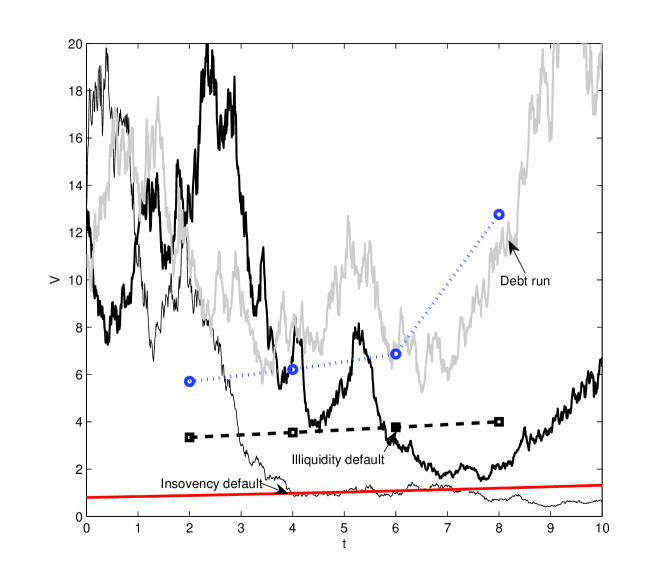
Figure 3: Scenario simulation with discrete tenor structure
The figure shows three simulated asset value paths in the model with a discrete tenor structure, where volatility $\sigma=0.4$, expected return rate $r_{V}=-0.02$, market interest rate $r=0.01$, short-term rate $r_{S}=0.03$, and long-term rate $r_{L}=0.05$. The initial values of short- and long-term debt are set to $S_{0}=2$ and $L_{0}=2$, respectively. The safety covenant parameter $\beta=0.4$, the bankruptcy cost parameter $\alpha=0.6$, and the fire-sale rate is set to $\psi=0.6$. The time horizon is $T=10$ years. In this discrete tenor structure setting the number of rollover dates is set to $N=4$. The dotted line describes the debt run barrier, the dashed line the illiquidity barrier, and the solid line the insolvency barrier.

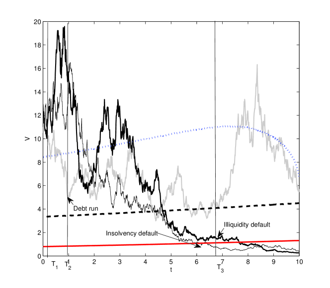
Figure 4: Scenario simulation with a staggered tenor structure
The figure shows three simulated asset value paths in the model with a staggered tenor structure where volatility $\sigma=0.4$, expected return rate $r_{V}=-0.02$, market interest rate $r=0.01$, short-term rate $r_{S}=0.03$, and long-term rate $r_{L}=0.05$. The initial values of short- and long-term debt are set to $S_{0}=2$ and $L_{0}=2$, respectively. The safety covenant parameter $\beta=0.4$, the bankruptcy cost parameter $\alpha=0.6$, and the fire-sale rate is set to $\psi=0.6$. The time horizon is $T=10$ years. In this staggered tenor structure setting the intensity of the Cox process is chosen to be $g(X_{t})\equiv 0.4$. The dotted line describes the debt run barrier, the dashed line the illiquidity barrier, and the solid line the insolvency barrier.

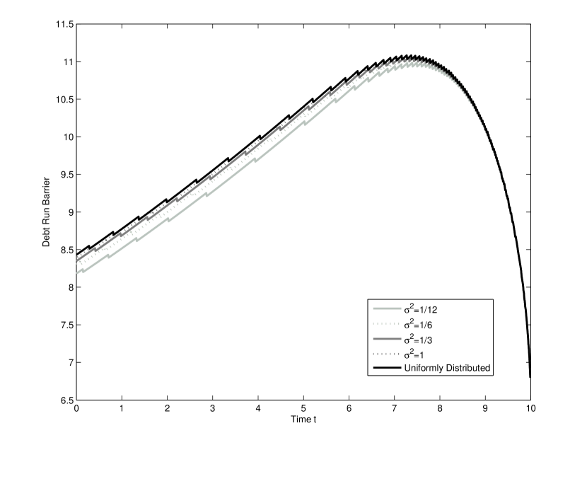
Figure 5: Comparison of debt run barriers with different assumptions on $\xi$
The figure shows debt run barriers with different assumptions on the random variable $\xi$, the creditor’s belief on the proportion of short-term creditors not rolling over their funding at each rollover date. The top line corresponds to the uniformly distributed $\xi$, and from the second top to the bottom lines, they correspond to the truncated normal distribution with mean $0.5$ and diminishing variances. Other parameters are the same as in Figure 4.

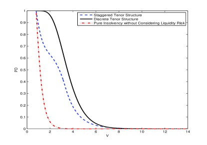
(a) For $\sigma=0.2$ and $g(x)=0.2$

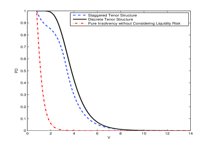
(b) For $\sigma=0.2$ and $g(x)=0.4$

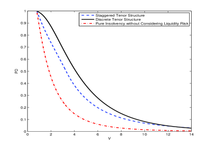
(c) For $\sigma=0.4$ and $g(x)=0.2$

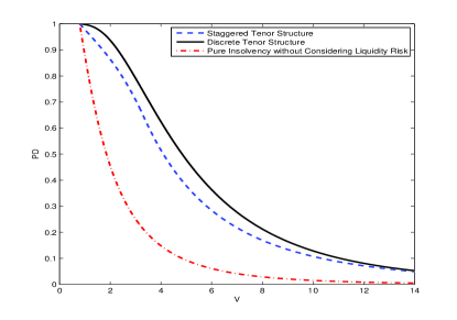
(d) For $\sigma=0.4$ and $g(x)=0.4$

Figure 6: Default probabilities under the discrete and the staggered tenor structure models
The figure shows the default probabilies under the discrete tenor structure and the staggered tenor structure. The dotted line is the default probability without including rollover risk. Other parameters are the same as in Figure 3 and Figure 4 apart from $T=5$ and $r_{V}=0.07$ and with volatility $\sigma$ and intensity $g(x)$ as specified below the graphs.

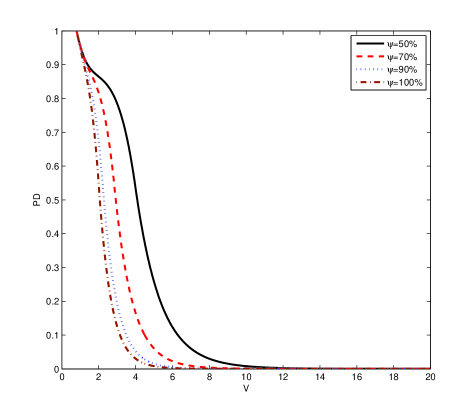
(a) For $\sigma=0.2$ and $g(x)=0.4$

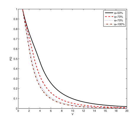
(b) For $\sigma=0.4$ and $g(x)=0.2$

Figure 7: Default probabilities for different fire-sale rates
The figure shows the default probabilies for different fire-sale rates. Other parameters are the same as in Figure 3 and Figure 4 apart from $T=5$ and $r_{V}=0.07$ and with volatility $\sigma$ and intensity $g(x)$ as specified below the graphs.

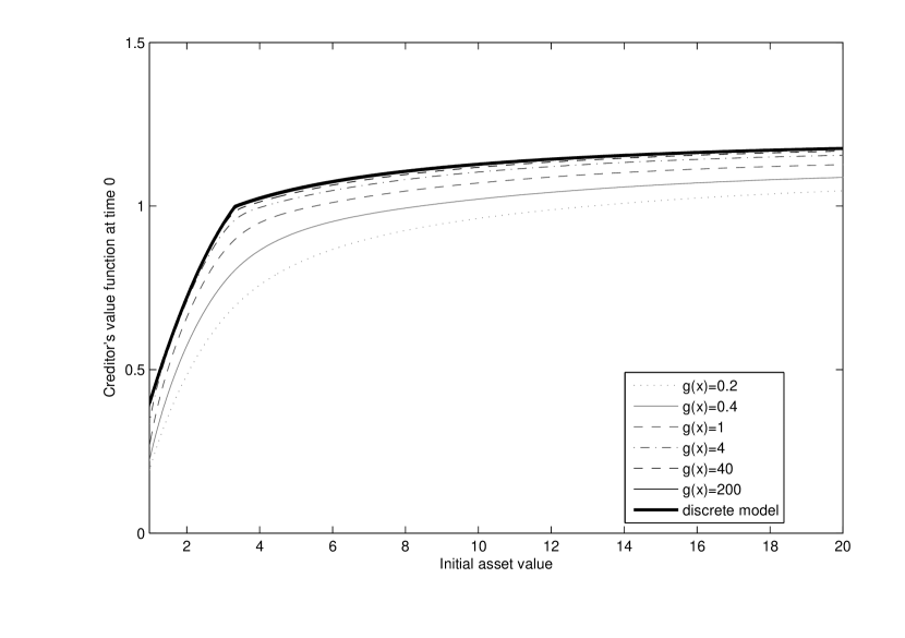
Figure 8: Influence of the intensity on creditor’s value function
The figure shows the representative creditor’s value function at time $t=0$ for increasing initial asset value $V_{0}$ in the discrete tenor structure model with $N=1000$ rollover dates and for the staggered tenor structure model for different intensities $g$ of the Cox process. Other parameters are the same as in Figure 4.

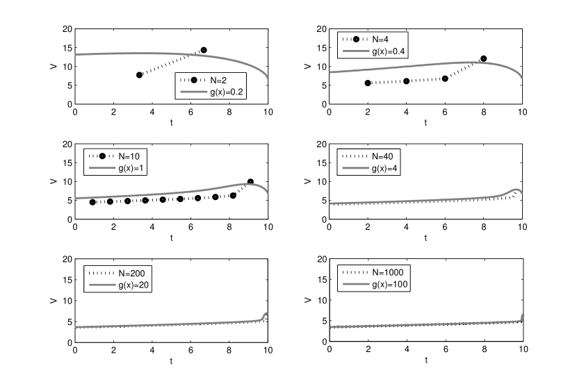
Figure 9: Comparison between the discrete and the staggered tenor structure models
The figure shows the debt run barrier depending on time $t$ for different rollover frequencies $N$ in the discrete tenor structure model and for different intensities $g(x)$ of the Cox process in the staggered tenor structure model. Other parameters are the same as in Figure 4.

References

- Adrian and Shin (2008) Adrian, T., and Shin, H.S. (2008): Liquidity and financial contagion. Financial Stability Review, Special issue on liquidity, No. 11, Banque de France.
- Adrian and Shin (2010) Adrian, T., and Shin, H.S. (2010): Liquidity and leverage. Journal of Financial Intermediation 19(3), 418–437.
- Arifovic et al. (2013) Arifovic, J., Jiang, J.H., and Xu, Y. (forthcoming): Experimental evidence of bank runs as pure coordination failures. Journal of Economic Dynamics and Control.
- Bielecki and Rutkowski (2002) Bielecki, T.R., and Rutkowski, M. (2002): Credit risk: Modeling, valuation and hedging. Springer.
- Black and Cox (1976) Black, F. and Cox, J. (1976): Some effects of bond indenture provisions. Journal of Finance 31, 351–367.
- Briys and de Varenne (1997) Briys, E. and de Varenne, F. (1997): Valuing risky fixed rate debt: An extension. Journal of Financial and Quantitative Analysis 32, 239–249.
- Brunnermeier (2009) Brunnermeier, M. (2009): Deciphering the liquidity and credit crunch 2007-08. Journal of Economic Perspectives 23, 77–100.
- Chen and Kou (2009) Chen, N. and Kou, S. (2009): Credit spread, implied volatility, and optimal capital structures with jump risk and endogenous defaults, Mathematical Finance, 19, 343–378.
- Cheng and Milbradt (2012) Cheng, I. H. and Milbradt, K. (2012): The hazards of debt: Rollover freezes, incentives, and bailouts. Review of Financial Studies 25(4), 1070–1110.
- Crépy et al (2012) Crépey, S., Grbac, Z. and Nguyen, H.N. (2012): A multiple-curve HJM model of interbank risk. Mathematics and Financial Economics 6(3) 155-190.
- Diamond and Dybvig (1983) Diamond, D. and Dybvig, P. (1983): Bank runs, deposit insurance and liquidity. Journal of Political Economy 91, 401–419.
- Ericsson and Renault (2006) Ericsson, J. and Renault, O. (2006): Liquidity and credit risk. Journal of Finance 61, 2219–2250.
- Goldstein and Pauzner (2005) Goldstein, I. and Pauzner, A. (2005): Demand-deposit contracts and the probability of bank runs. Journal of Finance 60, 1293-1327.
- He and Xiong (2012a) He, Z. and Xiong, W. (2012): Rollover risk and credit risk. Journal of Finance 67, 391–429.
- He and Xiong (2012b) He, Z. and Xiong, W.(2012): Dynamic debt runs. Review of Financial Studies 25 (6), 1799–1843.
- Hilberink and Rogers (2002) Hilberink, B. and Rogers, L.C.G. (2002): Optimal capital structure and endogenous default. Finance and Stochastics 6, 237–263.
- Krylov (2008) Krylov, N.V. (2008): Controlled diffusion processes. Springer, 2nd printing edition.
- Leland (1994) Leland, H.E. (1994): Corporate debt value, bond covenants, and optimal capital structure. Journal of Finance 49, 1213–1252.
- Leland (1998) Leland, H.E. (1998): Agency costs, risk management, and capital structure. Journal of Finance 53, 1213–1243.
- Leland and Toft (1996) Leland, H.E. and Toft, K. (1996): Optimal capital structure, endogenous bankruptcy, and the term structure of credit spreads. Journal of Finance 51, 987–1019.
- Liang (2013) Liang, G. (2013): Stochastic control representations for penalized backward stochastic differential equations, Working paper.
- Liang and Jiang (2012) Liang, G. and Jiang, L. (2012): A modified structural model for credit risk. IMA Journal of Management Mathematics 23, 147–170.
- Liang et al. (2014) Liang, G., Lütkebohmert, E. and Xiao, Y. (2014): A multi-period bank run model for liquidity risk. Review of Finance 18(2), 803–842.
- Longstaff and Schwartz (1995) Longstaff, F. and Schwartz, E. (1995): A simple approach to valuing risky fixed and floating rate debt. Journal of Finance 50, 789-819.
- Merton (1974) Merton, R.C. (1974): On the pricing of corporate debt: The risk structure of interest rates. Journal of Finance 29, 449–470.
- Morris and Shin (2010) Morris, S. and Shin, H.S. (2010): Illiquidity component of credit risk. Working Paper.
- Morris and Shin (2003) Morris, S. and Shin, H.S. (2003): Global Games: Theory and Applications. in Advances in Economics and Econometrics (Proceedings of the Eighth World Congress of the Econometric Society), edited by M. Dewatripont, L. Hansen and S. Turnovsky, Cambridge University Press.