Expander-like Codes based on Finite Projective Geometry

Abstract

We present a novel error correcting code and decoding algorithm which have construction similar to expander codes. The code is based on a bipartite graph derived from the subsumption relations of finite projective geometry, and Reed-Solomon codes as component codes. We use a modified version of well-known Zemor’s decoding algorithm for expander codes, for decoding our codes. By derivation of geometric bounds rather than eigenvalue bounds, it has been proved that for practical values of the code rate, the random error correction capability of our codes is much better than those derived for previously studied graph codes, including Zemor’s bound. MATLAB simulations further reveal that the average case performance of this code is 10 times better than these geometric bounds obtained, in almost 99% of the test cases. By exploiting the symmetry of projective space lattices, we have designed a corresponding decoder that has optimal throughput. The decoder design has been prototyped on Xilinx Virtex 5 FPGA. The codes are designed for potential applications in secondary storage media. As an application, we also discuss usage of these codes to improve the burst error correction capability of CD-ROM decoder.

Keywords:  Expander Codes, Bipartite Graph, Finite Projective Geometry.

1 Introduction

Graph codes have been studied and analyzed in past, in order to try and find codes that give good error correction capability at high code rates [1], [2], [3]. At the same time, from a practical implementation point of view, such codes require to have decoding and encoding algorithms that are efficient in terms of speed and hardware complexity.

Expander Codes, first suggested by Sipser and Spielman [4], proved to be theoretically capable of providing asymptotically good codes that were decodable in logarithmic time and could be implemented with a circuit whose size grew linearly with code size. These codes are constructed using a special graph, known as expander graph, and by embedding identical component codes at the nodes of this graph. [4] analyzed the properties of expander codes, and specified lower bound on the number of errors that will always be corrected by one decoding algorithm. Zemor, in his analysis in [3], suggested using bipartite Ramanujan graphs for constructing expander codes. He also provided a decoding algorithm which improved the lower bound in [4] by a factor of 12. In [1], Hoholdt and Justesen built on the work of Tanner on graph codes, by suggesting the use of Reed Solomon codes as sub-codes for graphs derived from point-line incidence relations of projective planes. The decoding speed and ease of implementation, combined with error-correction performance that was scalable with increasing graph size made all these codes interesting, while considering applications related to secondary storage.

By definition, the sub-code length should remain constant, as the order of (bipartite) expander graph increases, during construction of a family of expander codes. For performance reasons described later, we choose to increase the sub-code length as well. Hence our codes may not be called expander codes, but just graph-based, or expander-like codes. The presented work thus deals with the construction and analysis of an expander-like code, which is based on a special bipartite Ramanujan graph. This bipartite graph is derived from point-hyperplane incidence relations of projective spaces of higher dimensions than those suggested by [1]. We look at various properties of the codes, and in the process come across several generic interesting properties of projective geometry. Also, we wanted the codes to be practically useful. Hence, in a companion paper, we present throughput-optimal VLSI design of decoder for such codes[5].

For decoding, we employ a variation of Zemor’s algorithm. By simulations using this algorithm, we found that the codes have excellent robustness to random as well as burst errors. Hence we envisage their application in data storage systems.

The next section provides the basic properties of cardinalities of projective geometry that we will be using. Section 3 gives relevant background information for the various concepts required in this paper. Section 4 describes our code construction in detail. Sections 5-11 give the characterization of error-correction capability for these codes, including proofs of propositions relating to bounds on error correction capacity. The remaining sections detail out the prototyping results, and also the application to two types of storage media (namely CD-ROMs and DVD-R), before concluding the paper.

2 Finite Projective Spaces

In this section, we look at how finite projective spaces are generated from finite fields. For more details, refer [6]. Consider a finite field $\mathbb{F}=$ $\mathbb{GF}(s)$ with $s$ elements, where $s$ is a power of a prime number $p$ i.e. $s=p^{k}$, $k$ being a positive integer. A projective space of dimension $d$ is denoted by ${\mathbb{P}}(d,\mathbb{F})$ and consists of one-dimensional subspaces of the $(d+1)$-dimensional vector space over $\mathbb{F}$ (an extension field over $\mathbb{F}$), denoted by $\mathbb{F}^{d+1}$. Elements of this vector space are of the form $(x_{1},\ldots,x_{d+1})$, where each $x_{i}\in\mathbb{F}$. The total number of such elements are $s^{(d+1)}$ = $p^{k(d+1)}$. An equivalence relation between these elements is defined as follows. Two non-zero elements ${\bf{x}}$, ${\bf{y}}$ are equivalent if there exists an element $\lambda\in$ GF$(s)$ such that ${\bf{x}}=\lambda{\bf{y}}$. Clearly, each equivalence class consists of $s$ elements of the field ($s-1$ non-zero elements and ${\bf{0}}$), and forms a one-dimensional subspace. Such 1-d vector subspace corresponds to a point in the projective space. Points are the zero-dimensional subspaces of the projective space. Therefore, the total number of points in ${\mathbb{P}}(d,\mathbb{F})$ are

$$P(d) = \frac{\textrm{\# non-zero elements in the field}}{\textrm{\# non-zero elements in one equivalence class}}$$ (1)

$$= \frac{s^{d+1}-1}{s-1}$$ (2)

An $m$-dimensional subspace of ${\mathbb{P}}(d,\mathbb{F})$ consists of all the one-dimensional subspaces of an $(m+1)$-dimensional subspace of the vector space. The basis of this vector subspace will have $(m+1)$ linearly independent elements, say $b_{0},\ldots,b_{m}$. Every element of this subspace can be represented as a linear combination of these basis vectors.

$${\bf{x}}=\sum_{i=0}^{m}\alpha_{i}b_{i},\textrm{ where }\alpha_{i}\in\mathbb{F}(s)$$ (3)

Clearly, the number of elements in the vector subspace are $s^{(m+1)}$. The number of points in the $m$-dimensional projective subspace is given by $P(m)$ defined in earlier equation. Various properties such as degree etc. of a $\mathbf{m}$-dimensional projective subspace remain same, when this subspace is bijectively mapped to some $(\mathbf{d-m-1})$-dimensional projective subspace. The two sets of these subspaces, one for each dimension, are said to be dual of each other. The number of d-dimensional projective subspaces of a m-dimensional projective space can be counted using the Gaussian Coefficient.

$$\phi(n,l,s)=\frac{(s^{n+1}-1)(s^{n}-1)\ldots(s^{n-l+1}-1)}{(s-1)(s^{2}-1)\ldots(s^{l+1}-1)}$$ (4)

For $0\leq l<m\leq d$, the number of $\mathbf{l}$-dimensional projective subspaces contained in an $\mathbf{m}$-dimensional projective subspace is $\phi(m,l,s)$, while the number of $\mathbf{m}$-dimensional projective subspaces containing a particular $\mathbf{l}$-dimensional projective subspace is $\phi(d-l-1,m-l-1,s)$.

2.1 Projective Spaces as Lattices

It is a well-known fact that the lattice of subspaces in any projective space is a modular, geometric lattice [6]. A projective space of dimension 2 is shown in figure 1b. In the figure, the top-most node represents the supremum, which is a projective space of dimension m in a lattice for $\mathbb{P}(\mathbf{m},\mathbb{GF}(\mathbf{q}))$. The bottom-most node represents the infimum, which is a projective space of (notational) dimension -1. Each node in the lattice as such is a projective subspace, called a flat. Each horizontal level of flats represents a collection of all projective subspaces of $\mathbb{P}(\mathbf{m},\mathbb{GF}(\mathbf{q}))$ of a particular dimension. For example, the first level of flats above infimum are flats of dimension 0, the next level are flats of dimension 1, and so on. Some levels have special names. The flats of dimension 0 are called points, flats of dimension 1 are called lines, flats of dimension 2 are called planes, and flats of dimension (m-1) in an overall projective space $\mathbb{P}(\mathbf{m},\mathbb{GF}(\mathbf{q}))$ are called hyperplanes.

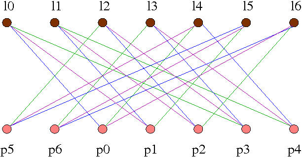
(a) PG graph

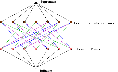
(b) Corresponding Lattice Diagram

Figure 1: An Example PG Bipartite Graph

3 Expander Codes

Expander codes are a family of asymptotically good, linear error-correcting codes [4]. They can be decoded in sub-linear time(proportional to log(n), where n is length of codeword) using parallel decoding algorithms. Further, this can be achieved using identical component decoders, whose count is proportional to n. These codes are based on a class of graphs known as expander graphs. One construction of expander graph, used in construction of expander codes, is by considering the edge-vertex incidence graph $\mathbb{Z}$ of a d-regular graph $\mathbb{G}$. The edge-vertex incidence graph of $\mathbb{G=(V,E)}$, a (2,d)-regular bipartite graph, has vertex set $E\cup V$ and edge set

$$\left\{(e,v)\in E\times V:\;\mbox{v is an endpoint of e}\right\}$$

Vertices of $\mathbb{Z}$ corresponding to edges E of $\mathbb{G}$ are then associated to variables, while vertices of $\mathbb{Z}$ corresponding to vertices of $\mathbb{G}$ are associated to constraints on these variables. Each constraint corresponds to a set of linear restrictions on the d variables that are its neighbors. In particular, a constraint will require that the variables it restricts form a codeword in some linear code of length d. This constraint forms the sub-code for that expander code. Further, all the constraints are required to impose isomorphic codes (on different variables, of course). The default construction of a family of expander codes requires d to remain constant, as the order of $\mathbb{G}$ increases.

Formally, Let $\mathbb{Z}$ be a (2,d)-regular graph between set of n nodes called variables, and $\frac{2}{d}$n nodes called constraints. Let z(i,j) be a function such that for each constraint $C_{i}$, the variables neighboring $C_{i}$ are $v_{z(i,1)},\cdots,v_{z(i,d)}$. Let $\mathbb{S}$ be an error-correcting code of block length d. The expander code $\mathbb{C(Z,S)}$ is the code of block length n whose codewords are the words $(x_{1},\cdots,x_{n})$ such that, for 1 $\leq$ $i$ $\leq$ $\frac{2}{d}$n, $x_{z(i,1)},\cdots,x_{z(i,d)}$ is a codeword of $\mathbb{S}$.

3.1 Expander Graphs

An expander graph is a graph in which every set of vertices has an unusually large number of neighbors. More formally,
Let $\mathbb{G}$ = ($\mathbb{V,E}$) be a graph with n vertices. Then the graph $\mathbb{G}$ is a $\delta$-expander, if every set of at most m vertices expands by a factor of $\delta$. That is,

$$\forall S\subset V:\left|S\right|\leq m\Rightarrow\left|\left\{y:\exists x\in S\mbox{ s.t. }(x,y)\in E\right\}\right|>\delta\cdot\left|S\right|$$

Expander codes being a subclass of LDPC codes, for whom efficient iterative decoding using variables and constraints a bipartite graph is feasible, we are interested mainly in bipartite expander graphs.

The degree of “goodness” of expansion, especially for regular graphs, can also be measured using its eigenvalues. The largest eigenvalue of a k-regular graph is k. If the second largest eigenvalue is much smaller from the first (k), then the graph is known to be a good expander [4].

3.2 Good Expander Codes

As pointed out earlier, the decoding algorithm for such codes is iterative. Hence good expander codes imply at least the following properties.

• Better minimum distance than other codes of same length,

• Fast convergence, and

• Better code rate than other codes in the same class

Good codes having the above properties can be identified with help of three theorems proved in [4]. For the theorems, we assume that an expander code $\mathbb{C(Z,S)}$ has been constructed having $\mathbb{S}$ as a linear code of rate r, block length d, and minimum distance $\epsilon$, and $\mathbb{Z}$ as the edge-vertex incidence graph of a d-regular graph $\mathbb{G}$ with second-largest eigenvalue $\lambda$.

Theorem 1.

The code $\mathbb{C(Z,S)}$ has rate at least 2r - 1, and minimum relative distance at least $\left(\frac{\epsilon-\frac{\lambda}{d}}{1-\frac{\lambda}{d}}\right)^{2}$.

Theorem 2.

If a parallel decoding round for $\mathbb{C(Z,S)}$, as given in [4], is given as input a word of relative distance $\alpha$ from a codeword, then it will output a word of relative distance at most $\alpha\left(\frac{2}{3}+\frac{16\alpha}{\epsilon^{2}}+\frac{4\lambda}{\epsilon d}\right)$ from that codeword.

Theorem 3.

For all $\epsilon$ such that 1- 2H($\epsilon$) $>$ 0, where H($\cdot$) is the binary entropy function, there exists a polynomial-time constructible family of expander codes of rate 1 - 2H($\epsilon$) and minimum relative distance arbitrarily close to $\epsilon^{2}$ in which any $\alpha$ $<$ $\epsilon^{2}$/48 fraction of error can be corrected by a circuit of size O(n log n) and depth O(log n).

From theorem 1, we observe that to have high minimum relative distance, we should have $\epsilon$ as high, and $\frac{\lambda}{d}$ as low. Since $\mathbb{Z}$ has been constructed out of d-regular graph $\mathbb{G}$, low $\frac{\lambda}{d}$ signifies high distance between first and second eigenvalues, i.e. the graph $\mathbb{G}$ has to be a “good” expander graph. Further, to have high rate, $\mathbb{S}$ has to have a high rate r as well, other than having high minimum relative distance $\epsilon$.

From theorem 2, we observe that to shrink the distance of input word after one iteration maximally, we need to again have $\epsilon$ as high as possible, and $\frac{\lambda}{d}$ as low as possible. Such maximal shrinking of distance, per iteration, leads to the fastest convergence possible, as is also brought out in the proof of theorem 3.

From theorem 3, we observe that to be able to correct as high fraction of errors as possible, we need to have $\epsilon$ as high as possible, again.

As an aside, $\frac{\lambda}{d}$ is low whenever d is high. In PG-based bipartite graphs, d does increase, as n increases (hence expander-like codes), which hence helps in making the overall code advantageous over classical expander codes.

3.3 Good Expander Graphs

Zemor pointed out [3] that if $\mathbb{G}$ is a bipartite graph, then the % of random errors that can be corrected using a parallel iterative decoding algorithm can be increased twelve-fold. He also pointed out that the upper bound on minimum distance, as pointed out in theorem 1, can also be achieved faster, if one considers Ramanujan graphs (since $\frac{\lambda}{d}$ value is low for these graphs). Overall, he suggested using bipartite Ramanujan graphs for construction of good expander codes instead.

4 Details of Expander-like Code

4.1 PG Graphs as Good Expander Graphs

Balanced regular bipartite graphs $G_{d,d}$, which are symmetric balanced incomplete block designs(BIBDs) are known to be Ramanujan graphs [2]. Incidence relations of projective geometry structures give such BIBDs, and hence Ramanujan graphs. Usage of projective plane as $G_{d,d}$ along with RS codes as component codes to construct good expander-like graph codes was first reported in [1]. For our work, we do not limit to projective planes: to have better performance, we have made use of point-hyperplane incidence graphs from higher dimensional projective spaces, which also satisfy the eigenvalue properties that make a Ramanujan graph. Some reasons for using projective geometry are as follows.

• As detailed in a companion paper [5], the mapping of vertices to points and hyperplanes enables us to use several projective geometry properties for disproving the existence of certain bipartite subgraphs of a fixed minimum degree. This strategy leads us to finding the minimum number of vertices required to form a complete bipartite subgraph of a given minimum degree. This number of vertices is required to calculate tight geometric bounds for error correction capability of the overall code. Thus, we don’t need to use complicated eigenvalue arguments used by [4] and [3]. Also, the bounds obtained in this manner are better than our predecessors. Furthermore, Zemor had restricted the subcodes to be constrained by $d\geq 3\lambda$, $\lambda$ being the second largest eigenvalue of the graph. We have no such restriction.

• The use of projective geometry also helps in developing a perfect folded architecture of the decoder for hardware implementation, discussed later in section 10. This particular folding enables efficient utilization of processors and memories, while being throughput-optimal.

4.2 Reed-Solomon Codes as Good Component Codes

By choosing a “good expander” graph, and fixing a code with high minimum relative distance $\epsilon$, one can design code having the first two properties described in section 3.2. To simultaneously have high code rate for $\mathbb{C(Z,S)}$, the component code $\mathbb{S}$ also needs to have high rate r. Reed-Solomon codes are a class of non-binary, linear codes, which for a given rate, have the best minimum relative distance(so-called maximum distance separable codes), and vice-versa. Hence we use RS codes as the sub-codes to our expander-like codes.

4.3 Code Construction

To construct an expander-like code, we follow [3]. We generate a balanced regular bipartite graph $\mathbb{G}$ from a projective space. A projective space of dimension n over $\mathbb{GF}(2)$, $\mathbb{P}(n,\mathbb{GF}(q))$, has at least following two properties, arising out of inherent duality:

1. The number of subspaces of dimension $m$ is equal to the number of subspaces of dimension ($n-m-1$).

2. The number of $m$-dimensional subspaces incident on each ($n-m-1$)-dimensional subspace is equal to the number of ($n-m-1$)-dimensional subspaces incident on each $m$-dimensional subspace.

We associate one vertex of the graph with each $m$-dimensional subspace and one with each ($n-m-1$)-dimensional subspace. Two vertices are connected by an edge if the corresponding subspaces are incident on each other. As edges lie only between subspaces of different dimensions, the graph is bipartite with vertices associated with $m$-dimensional subspaces forming one set and vertices associated with ($n-m-1$)-dimensional subspaces forming another. Also, the two properties, listed above, ensure that both the vertex sets have the same number of elements and that each vertex has the same degree. To be able to quantify various properties of the constructed code, we hereafter specifically consider the graph, $\mathbb{G}=(V,E)$, obtained by taking the points and hyperplanes of $\mathbb{P}(5,\mathbb{GF}(2))$. In this projective space, the number of points (= number of hyperplanes) is $\phi(5,0,2)=63$. Each point is incident on $\phi(4,3,2)=31$ hyperplanes and each hyperplane has $\phi(4,0,2)=31$ points. Therefore, we have $|V|=126$ and $|E|=1953$. This implies that the block length of code $\mathbb{C}$ is $1953$ and the number of constraints in the code is $126$. The second eigenvalue of $\mathbb{G}$, $\lambda$ is 4, according to a formulae by [7]. Hence the ratio $\frac{\lambda}{d}$ is quite small, as required for design of “good” expander codes.

As the expander graph $\mathbb{G}$ is $31$-regular, the block length of the component code must also be $31$ [4]. We choose the $31$-symbol shortened Reed Solomon code as the component code, with each symbol consisting of eight bits. To have performance advantage, we also modify Zemor’s decoding algorithm [3] as follows. If a particular vertex detects more errors than it can correct, we skip the decoding for that vertex. In Zemor’s algorithm, the decoding is still carried out in such case, which can lead to possibly getting a (different) codeword with more errors. The modification is possible because it is possible to compute, as a side output using Berlekamp-Massey’s algorithm for RS decoding[8], whether the degree of errors in the current input block of symbols to the decoder be corrected or not. If not, then the algorithm can be made to skip decoding, thus preserving the errors in the input block. This variation in decoding will reduce the number of extra errors introduced by that vertex if the decoding fails. Based on this decoding algorithm, a MATLAB model of decoder was first made, to observe code’s performance as discussed next.

5 Performance of Code for Random Errors

To benchmark the error-correction performance in wake on random errors, we varied the minimum distance of the component code, and simulated the MATLAB decoder model. Random symbol errors were introduced at random locations of the zero vector. Convergence of the decoder’s output back to the zero vector was checked after simulation. As our code is linear, the performance obtained in testing for zero vector is valid for the entire code. Since the errors were introduced at random locations, simulations were run over many different rounds of decoding for different pseudo-random sequences as inputs, and averaged, to get reliable results. These sequences differ in random positions in which the errors are introduced. Each round of decoding for particular input further involves several iterations of execution of decoding algorithm. One iteration of decoding corresponds to both sides of the bipartite graph to finish decoding the component codes.

It is observed experimentally that in case of a decoding failure, beyond 4 iterations, the number of errors in the codeword stabilizes(referred to as fixed point in [9]). In the first few iterations, as the number of errors decrease in the overall code in a particular iteration, the number of errors on average to be handled by RS decoders in next iteration is lesser. Hence probabilistically, and experimentally, these component decoders converge faster, thus increasing the percentage of errors being corrected in its next iteration. However, after maximum 4 iterations, it was seen that there is no further reduction in errors. This phenomenon could most probably be attributed to infinite oscillations of errors in an embedded subgraph, to be described in next section.

Hence we have fixed the stopping threshold of decoder to exactly 4 iterations not only in simulation, but also in the practical design of a CD-ROM decoder. In simulation, if there are non-zero entries remaining after 4 iterations, then the decoding is considered to have failed. In real life, if one or more component RS decoders fail to converge at 4th iteration, then again decoding is considered to have failed. The results of our simulations are presented in Tables 1 and 2. The component codes used for these simulations have minimum distance as 5 and 7, respectively. The “failures” column represents the percentage of failed decoding attempts. The “average number of iterations” column signifies the average number of iterations required for successful decoding of a corrupt codeword, over various rounds.

No. of errors	failures	Avg. no. of iterations
50	0	1
80	1	1.71
100	18	2.33
110	40	2.72

Table 1: Random errors ($\epsilon=5$)

No. of errors	failures	Avg. no. of iterations
150	0	1.6
175	0	1.99
200	0	2.19
250	23	3.82
275	64	4.5

Table 2: Random errors ($\epsilon=7$)

We present some worst-case bounds on rate and error-correction capability of our codes in Table 3. We vary the minimum distance of subcode between 3 and 15. Beyond 15, rate of the overall code $\mathbb{C}$ becomes very less and hence impractical. We also compare these bounds to the bounds derived by Zemor. For calculating the Zemor bounds and making a fair comparison, we need to remove the advantage of using Reed Solomon codes as sub-codes. Zemor had derived the bounds for general codes assuming that $\geq$ $\frac{\epsilon}{2}$ errors could not be corrected for any distance(even/odd). For Reed Solomon component codes used in our construction, since we use only odd distances, $\frac{(\epsilon+1)}{2}$ errors can never be corrected. To account for this, we replace $\epsilon/2$ by $(\epsilon+1)/2$ in Zemor’s formula to calculate the bounds.

Min. dist.	Subcode	Lower bound	Error-correcting	Zemor’s
subcode $(\epsilon)$	rate	on rate of $\mathbb{C}$	capability	bound
$(\epsilon)$			of $\mathbb{C}$	for $\mathbb{C}$
3	0.94	0.87	3	–
5	0.87	0.74	8	–
7	0.81	0.61	15	–
9	0.74	0.48	24	–
11	0.68	0.35	35	–
13	0.61	0.23	48	42
15	0.55	0.1	87	65

Table 3: Change in parameters of $\mathbb{C}$ with variation in minimum distance of subcode

We give a geometrical analysis of process of error correction in the overall code $\mathbb{C}$. We have also used results from this analysis to derive the bounds on error correction capability of $\mathbb{C}$. First of all, since we have $\mathbb{P}(5,\mathbb{GF}(2))$, points form the 0-dimensional subspace and hyperplanes form the 4-dimensional subspace. Moreover, planes form 2-dimensional subspaces of the projective space, and are symmetric with respect to points and hyperplanes. Finally, 7 points are contained in a plane and a plane is contained in 7 hyperplanes in $\mathbb{P}(5,\mathbb{GF}(2))$.

To understand the limits, given the minimum distance $\epsilon$ of the subcode, we need to find the minimum number of random errors to be introduced in $\mathbb{C}$, which will cause the decoding to fail. This will happen if the vertices corresponding to the points and hyperplanes get locked in such a way that in each iteration, an equal number of constraints fail on each side. This is the minimal configuration of failure. As explained next, errors can expand over iterations(more edges represent corrupt symbols), but that is not the minimum configuration of failure. Similarly, if errors shrink, i.e. lesser number of vertices in bipartite graph fail in next iteration, then it leads to a case of decoding convergence, not decoding failure.

For example, if we consider $\epsilon=5$, each vertex of the graph can correct up to 2 erroneous symbols($\lfloor\frac{\epsilon}{2}\rfloor$) in the set of symbols that it is decoding. If 3 or more erroneous symbols are given to it, then either the decoder, based on Berlekamp-Massey’s algorithm, skips decoding, or it outputs another codeword that in worst case has at least $\epsilon$ different symbols now(than the transmitted codeword), and hence at least $\epsilon$ errors. However, as discussed earlier, we are not interested in the latter case. So, if we can generate a case in which decoding of the sub-code fails at vertices corresponding to 3 points, all of which are incident on 3 hyperplanes, we have a situation in which the 3 points will transfer at least 3 errors to each of vertices corresponding to the 3 hyperplanes. These vertices may also fail, or decode a different codeword, while decoding their inputs. Again in the worst case each of these hyperplane decoders will output at least 3 erroneous symbols. These corrupt symbols, or errors, are then transferred back to the vertices representing the 3 points. Thus, the errors will keep oscillating infinitely from one side of the graph to the other, and the decoder will never decode the right codeword. Thus, a minimum of $3*3=9$ errors are required to cause a failure of decoding. This can be seen from the figure 2.

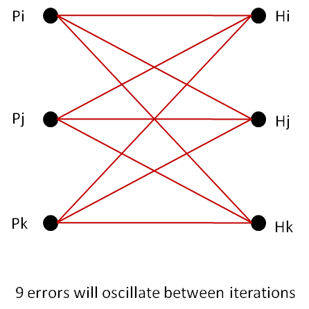
Figure 2: Subgraph that causes failure ($\epsilon=5$)

For any case in which less than 9 corrupt symbols exist, by pigeonhole principle, we will have at least one hyperplane or point having less than 3 errors incident on it. Decoder corresponding to that vertex will correctly decode the sub-code, thus reducing the total number of errors flowing in the overall decoder system of $\mathbb{C}$. This will, in next iteration, cause some other hyperplane or point to have less than 3 errors. Thus in the subsequent iterations, all the errors will definitely be removed. Therefore, 8 errors or less will always be corrected. This has been illustrated in figure 3.

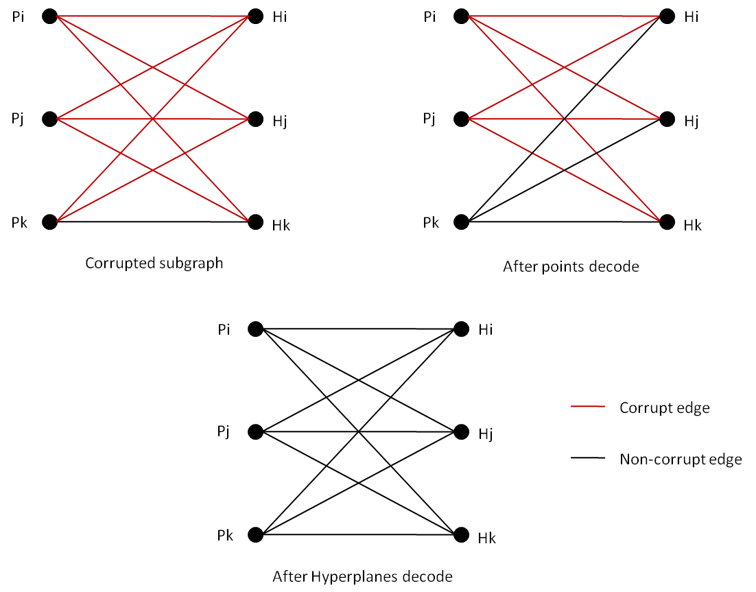
Figure 3: 8 or less errors always corrected

As we can see from Table  1, the worst case scenario is very unlikely to occur and for randomly placed errors, even 80 errors are found to be corrected 99% of the time.

Now the question is, when can we find a configuration in which 3 points are all incident on 3 hyperplanes? If we choose any plane in the given geometry, we can pick up any three points of that plane and find any 3 hyperplanes corresponding to the same plane. This will ensure that all the 3 points are incident on all the 3 hyperplanes. Thus, if for some input, the decoding at these 3 points fails, in the worst case they will corrupt all the edges incident on them. This in turn would cause 3 errors each, on the chosen hyperplanes. Hence the errors would oscillate between points and hyperplanes for each successive iteration. Thus, in the worst case, there need to be 9 erroneous symbols, located such that they are incident on the 3 chosen points, to cause the decoding of $\mathbb{C}$ to fail.

In general, if we are given a minimum distance $\epsilon$ of the subcode, it is known that at each vertex, more than ($\frac{\epsilon+1}{2}$) errors will not be corrected. So, in our graph we need to find the minimum number of vertices $\xi$ required to get a embedded bipartite subgraph such that each vertex in the subgraph has a degree of at least ($\frac{\epsilon+1}{2}$) towards vertices on other side of the subgraph. Once this number of vertices in some embedded subgraph has been found, the number of errors that can always be corrected by our decoder is given by:

$$E=\xi(\frac{\epsilon+1}{2})-1$$

In $\mathbb{P}(5,\mathbb{GF}(2))$, a plane has 7 points, and is contained in 7 hyperplanes. For $3\leq\epsilon\leq 13$, $\epsilon$ being odd, the minimum number of vertices $\xi$ corresponds to ($\frac{\epsilon+1}{2}$), and the corresponding points and hyperplanes can be picked from any plane. For $\epsilon\geq 15$, the calculation of $\xi$ is non-trivial, since points and hyperplanes from one plane are not sufficient. This is because $\frac{\epsilon+1}{2}=8$, which would require us to get a subgraph of minimum degree 8. Construction of such embedded subgraph is not possible by choosing only one plane.In next few sections, we give detailed proof to show non-existence of a minimum degree 8 embedded bipartite subgraph having 9, 10 vertices on each side, within point-hyperplane graph of $\mathbb{P}(5,\mathbb{GF}(2))$. Assuming that a sub-graph with 11 vertices exists, having a vertex degree of at least 8 (we have not been able to disprove it yet), we get the bound stated in table 3 for $\epsilon=15$. Since our constructions are exact, we can use these tight lower bounds for all practical values of $\epsilon$, wherever calculation of it is possible. Otherwise, another looser, lower bound can be found using Lemma 1 of [1], but derivation of that uses eigenvalue calculations. Without that, it is still clear from this table that the bound is much better than the bound obtained by Zemor[3] using eigenvalue arguments.

5.1 Bound in case of $\epsilon=15$

Earlier in this section, we highlighted the method to analyze the error correction bounds for our code. We also derived the bounds for $3\leq\epsilon\leq 13$. For the complex case of $\epsilon=15$, we present in next few sections, overview of proofs for establishing the non-existence of certain sub-graph embeddings which help us improve the bound, as reflected in table 3. The detailed proofs are presented in Appendix A. Appendix B presents a eigenvalue based approach (similar to Zemor’s arguments).

We first describe the two theorems, that prove the non-existence of certain minimal embeddings.

Theorem 4.

In the construction of bipartite graph mentioned above, there exists no embedded subgraph having size of partitions as 9, the degree of each of whose vertices has a minimum degree($\delta$) of 8.

Theorem 5.

In the construction of bipartite graph mentioned above, there exists no embedded subgraph having size of partitions as 10, the degree of each of whose vertices has a minimum degree($\delta$) of 8.

6 Vector Space Representation of Geometry

In this section, we outline certain details used in the proofs of the above theorems, in Appendix A. To recall, the points of an $n$-dimensional projective space over a field $\mathbb{F}$ can be taken to be the equivalence classes of nonzero vectors in the (n + 1)-dimensional vector space over $\mathbb{F}$. Vectors in an equivalence class are all scalar multiples of one-another. These vector being one-dimensional subspaces, they also represent the rays of a vector space passing through origin. The orthogonal subspace of each such ray is the unique n-dimensional subspace of $\mathbb{F}^{n+1}$, known as hyperplanes. Each vector $h$ of such orthogonal subspace is linked to the ray, $p$, by a dot product as follows.

$$p_{0}h_{0}+p_{1}h_{1}+\cdots+p_{n}h_{n}=0$$

where $p_{i}$ is the $i^{th}$ coordinate of $p$. This uniqueness implies bijection, and hence a vector $p$ can be used to represent a hyperplane subspace, which is exclusive of this vector as a point. Due to duality, similar thing can be said about a hyperplane subspace.

Hereafter, whenever we say that two projective subspaces of same dimension are independent, we mean the linear independence of the corresponding vector subspaces in the overall vector space.

6.1 Relationship between Projective Subspaces

Throughout the remaining paper, we will be trying to relate projective subspaces of various types. We define the following terms for relating projective subspaces.

[Contained in]

If a projective subspace X is said to be contained in another projective subspace Y, then the vector subspace corresponding to X is a vector subspace itself, of the vector subspace corresponding to Y. In terms of projective spaces, the points that are part of X, are also part of Y. The inverse relationship is termed ‘contains’, e.g. “Y contains X”.

[Reachable from]

If a projective subspace X is said to be reachable from another projective subspace Y, then there exists a chain(path) in the corresponding lattice diagram of the projective space, such that both the flats, X and Y lie on that particular chain. There is no directional sense in this relationship.

7 Lemmas Used in Proof

In this section, we describe certain useful lemmas, related to proofs of theorems 4 and 5. These short lemmas and their proofs provide an insight into the way detailed proofs were built up for theorems 4 and 5, in appendix A.

7.1 Lemmas Related to Projective Space

Lemma 6.

In projective spaces over $\mathbb{GF}$(2), any subset of points(hyperplanes) having cardinality of 4 or more has 3 non-collinear(independent) points(hyperplanes).

Proof.

The underlying vector space is constructed over GF(2). Hence, any 2-dimensional subspace of contains the zero vector, and non-zero vectors of the form $\alpha a+\beta b$. Here, $a$ and $b$ are linearly independent one-dimensional non-zero vectors, and $\alpha$ and $\beta$ can be either 0 or 1:
$\alpha,\beta\;\in\;\mathbb{GF}(2):(\alpha\;=\;\beta)\;\neq\;0$.
Thus, any such 2-d subspace contains exactly 3 non-zero vectors. Therefore, in any subset of 4 or more points of a projective space over $\mathbb{GF}(2)$ (which represent one-dimensional non-zero vectors in the corresponding vector space), at least one point is not contained in the 2-d subspace formed by 2 randomly picked points from the subset. Thus in such subset, a further subset of 3 independent points(hyperplanes) i.e. 3 non-collinear vectors can always be found. ∎

Lemma 7.

Let there be 7 hyperplanes $H1,\cdots,H7$ reachable from a plane $P1$ in $\mathbb{PG}(5,\mathbb{GF}(2))$. Let there be any other plane $P2$, which may or may not intersect with the point set of plane $P1$. Then, any point on $P2$ which is not reachable from plane $P1$, can maximally be reachable from 3 of these 7 hyperplanes, and vice-versa. Further, these 3 hyperplanes cannot be independent. Dually, any hyperplane containing $P2$, and not containing $P1$, can maximally be reachable from 3 of the 7 points contained in $P1$ and which are not independent, and vice-versa.

Proof.

If a point on plane $P2$ which is not reachable from plane $P1$ lies on 4 or more hyperplanes(out of 7) reachable from plane $P1$, then by lemma 6, we can always find a subset of 3 independent hyperplanes in this set of 4. In which case, the point will also be reachable from linear combination of these 3 independent hyperplanes, and hence to all the 7 hyperplanes which lie on plane 1. This contradicts the assumption that the point under consideration does not lie on plane $P1$. The role of planes $P1$ and $P2$ can be interchanged, as well as roles of points and hyperplanes, to prove the remaining alternate propositions.   Hence if the point considered above lies on 3 hyperplanes reachable from $P1$, then these 3 hyperplanes cannot be independent, following the same argument as above. Otherwise it is indeed possible for such a point to lie on 3 hyperplanes, e.g. in the case of the planes $P1$ and $P2$ being disjoint. ∎

Lemma 8.

Let there be 7 hyperplanes $H1,\cdots,H7$ reachable from a plane $P1$ in $\mathbb{PG}(5,\mathbb{GF}(2))$. Further, let there be any other plane $P2$, which intersects $P1$ in a line. Then, there exist 4 hyperplanes reachable from plane $P1$ which do not contain any of the 4 points that are in plane $P2$, but not in plane $P1$.

Proof.

A line contains 3 points in $\mathbb{PG}(5,\mathbb{GF}(2))$. Hence, $P1$ and $P2$ intersect in 3 points. By duality arguments, they intersect in 3 hyperplanes as well. Hence, $P2$ contains 7-3 = 4 points that are not common to point set of $P1$. By lemma 7, these 4 points can at maximum lie on 3 hyperplanes reachable from plane $P1$. Since there are 3 hyperplanes common to $P1$ and $P2$, and hence these 4 points already lie on them, they do not further lie on any more hyperplane reachable from $P1$, but not from $P2$. ∎

Lemma 9.

Let there be 7 hyperplanes $H1,\cdots,H7$ reachable from a plane $P1$ in $\mathbb{PG}(5,\mathbb{GF}(2))$. Further, let there be any other plane $P2$, which intersects $P1$ in a point. By lemma 7, the 6 hyperplanes not containing both $P1$ and $P2$ still intersect $P2$ maximum in a line each. Then, (a) Such lines contain the common point to $P1$ and $P2$, and hence exactly 2 more out of remaining 6 points of $P2$ that are not common to $P1$, and (b) 3 pairs of hyperplanes out of the 6 non-common hyperplanes intersect in a (distinct) line each out of the 3 possible lines in $P2$ containing the common point.

Proof.

Let $A_{c}$ be the common atom(point) between planes $P1$ and $P2$. By duality, exactly one hyperplane will be common to both $P1$ and $P2$. Let some non-common hyperplane $H_{nc}$ reachable from plane $P1$ intersect plane $P2$ in a line $L1$, that is, $H_{nc}\cap P2=L1$. Then, $A_{c}\in L1$. For if it is not, then
$\left|L1\cap A_{c}\right|=4$
$\mbox{Also, }L1\cup A_{c}\subseteq H_{nc}$
$\mbox{and, }L1\cup A_{c}\subseteq P2$
$\Rightarrow\left|H_{nc}\cap P2\right|=4$, a contradiction to lemma 7. Hence, the line $L1$ contains common point $A_{c}$ and 2 more out of remaining 6 points of $P2$ that are not common to $P1$.  
Exactly 3 hyperplanes of the nature $H1$, $H2$, $H1+H2$ intersect in a 4-dimensional subspace, in $\mathbb{PG}(5,\mathbb{GF}(2))$. Such a subspace can always be formed by taking union of a plane and a line intersecting the plane in a point, by rank arguments. Let the common hyperplane to $P1$ and $P2$ be $H_{c}$. Let other hyperplanes reachable from $P1$ be $H1,H2,H1+H_{c},H2+H_{c},H1+H2,H1+H2+H_{c}$. Then, the pairs of hyperplanes $\langle$$H1,H1+H_{c}$$\rangle$, $\langle$$H2,H2+H_{c}$$\rangle$, and $\langle$$H1+H2,H1+H2+H_{c}$$\rangle$, along with $H_{c}$, form 3 distinct 4-d subspaces, which leads to 3 distinct lines of meet under plane $P2$, for each pair. This can also be verified from the fact that there are exactly 3 distinct lines in plane $P2$ that have a point $A_{c}$ in common. These 3 lines, and their individual unions with $P1$, leads to reachability from $H1,H_{c},H1+H_{c}$, $H2,H_{c},H2+H_{c}$, and $H1+H2,H_{c},H1+H2+H_{c}$, respectively. ∎

Lemma 10.

Let there be two hyperplanes $H1$ and $H2$ meeting in a plane $P1$. Both $H1$ and $H2$ intersect any plane $P2$ disjoint from $P1$ in exactly a line, by lemma 7. Then these intersecting lines $L1$(of $H1$ and $P2$) and $L2$(of $H2$ and $P2$) cannot be the same.

Proof.

Let the vector space of a projective geometry flat $X$ be denoted by $V(X)$. Flats are sets of points, each of which bijectively corresponds to a 1-d vector in the corresponding vector space. Also, closure of a flat(in terms of containing a point) is defined as corresponding closure of the vector subspace. Hence, family of substructures in a projective space is bijectively intertwined to the family of subspaces in the corresponding vector space. Then, if $L1$ = $L2$ were true, then

$$V(L1)\;=\;V(L2)$$ (5)

where

$$V(L1)\;=\;V(H1)\cap V(P2)$$ (6)

$$V(L2)\;=\;V(H2)\cap V(P2)$$ (7)

Also, it is given that

$$V(H1)\cap V(H2)\;=\;V(P1)$$ (8)

$$V(P1)\cap V(P2)\;=\;\phi$$ (9)

Hence if one takes closure of set of vectors contained in $V(L1)\cup V(P1)$ ($L1$ is part of $P2$ which does not intersect with $P1$), it does generate the entire vector subspace $V(H1)$. Similarly, closure of set of vectors contained in $V(L2)\cup V(P1)$ generates the entire vector subspace $V(H2)$. Then from equation 5, the generated subspaces $V(H1)$ and $V(H2)$ coincide, a contradiction. ∎

7.2 Lemmas Related to Embedded Graphs

Lemma 11.

In a bipartite graph having 9 vertices each in both partite sets, and having a minimum degree($\delta$) of at least 8, any collection of 3 vertices from one side is incident on at least 6 common vertices on the other side.

Proof.

Let the vertices of one side be denoted as (a1, a2, $\cdots$, a9), and that of other side by (b1, b2, $\cdots$, b9). Given $\delta$ = 8, it is obvious that minimal intersection of neighborhoods of a1 and a2 happens in some(at least) 7 vertices from the other side. Then the 2 remaining vertices are $N(a1)-N(a1)\cap N(a2)$ and $N(a2)-N(a1)\cap N(a2)$, respectively. The neighborhood of vertex a3 may either contain all these 7 vertices ($N(a1)\cap N(a2)$), or the two vertices $N(a1)-N(a1)\cap N(a2)$ and $N(a2)-N(a1)\cap N(a2)$, and at least 6 vertices out of $N(a1)\cap N(a2)$. Hence the minimal intersection of neighborhoods of arbitrarily chosen vertices a1, a2 and a3 is of cardinality 6. ∎

Lemma 12.

In a bipartite graph having 10 vertices each in both partite sets, and having a minimum degree($\delta$) of at least 8, any collection of 3 vertices from one side is incident on at least 4 common vertices on the other side.

Proof.

Let the vertices of one side be denoted as (a1, a2, $\cdots$, a9), and that of other side by (b1, b2, $\cdots$, b9). Given $\delta$ = 8, it is obvious that minimal intersection of neighborhoods of a1 and a2 happens in some(at least) 6 vertices from the other side. The two vertices in $N(a1)-N(a1)\cap N(a2)$ and two more in $N(a2)-N(a1)\cap N(a2)$ count the 4 remaining vertices on the other side. The neighborhood of vertex a3 may either contain all these 6 vertices ($N(a1)\cap N(a2)$), or at most all 4 vertices $N(a1)-N(a1)\cap N(a2)$ and $N(a2)-N(a1)\cap N(a2)$, and at least 4 vertices out of $N(a1)\cap N(a2)$. Hence the minimal intersection of neighborhoods of arbitrarily chosen vertices a1, a2 and a3 is of cardinality 4. ∎

Lemma 13.

In a bipartite graph having 11 vertices each in both partite sets, and having a minimum degree($\delta$) of at least 8, any collection of 3 vertices from one side is incident on at least 2 common vertices on the other side.

Proof.

Let the vertices of one side be denoted as (a1, a2, $\cdots$, a9), and that of other side by (b1, b2, $\cdots$, b9). Given $\delta$ = 8, it is obvious that minimal intersection of neighborhoods of a1 and a2 happens in some(at least) 5 vertices from the other side. The three vertices in $N(a1)-N(a1)\cap N(a2)$ and three more in $N(a2)-N(a1)\cap N(a2)$ count the 6 remaining vertices on the other side. The neighborhood of vertex a3 may either contain all these 5 vertices ($N(a1)\cap N(a2)$), or at most all 6 vertices $N(a1)-N(a1)\cap N(a2)$ and $N(a2)-N(a1)\cap N(a2)$, and at least 2 vertices out of $N(a1)\cap N(a2)$. Hence the minimal intersection of neighborhoods of arbitrarily chosen vertices a1, a2 and a3 is of cardinality 2. ∎

8 Performance of Code for Burst Errors

The strongest applications for this code lie in the areas of mass data storage such as discs. Here, as pointed earlier in section 1, burst errors are the dominant cause of data corruption. Hence we have also examined the burst error correction capabilities of our code.

In bipartite graph $\mathbb{G}$ constructed from $\mathbb{P}(5,\mathbb{GF}(2))$, we label the edges with integers, to map various symbols of the codeword. Such a labeling is not required to understand/ characterize the random error correction capability of the code. But here, we label the edges with numbers to try to maximize the burst error correction capability. This is achieved if each consecutive symbol, possibly part of a burst, is mapped to edges that are incident on distinct vertices representing different component decoders. Thus, consecutive numbered edges, representing consecutively located symbols in input symbol stream, go to different vertices hosting different RS decoders. Since there are 63 vertices on one side of the graph, this scheme of numbering implies that edges incident on vertex 1 are assigned the numbers {1, 64, …, 1890}. Similarly, the edges incident on Vertex 2 are assigned {2, 65, …, 1891}, and so on. This numbering essentially achieves the effect of interleaving of code symbols. If the error correcting capacity of each component RS decoder is $\mu$(= $\lfloor\frac{\epsilon}{2}\rfloor$), then the minimum burst error correcting capacity of $\mathbb{C}$ will be $\mu*63$. For example, for $\epsilon=5$, $\mu$ is 2, and the minimum burst error correcting capacity is $2*63=126$. Table 4 gives MATLAB simulation results for burst error correction for $\epsilon=5$.

No. of errors	failures	Avg. no. of iterations
126	0	1
135	26	2.43

Table 4: Burst errors ($\epsilon=5$)

To demonstrate the excellent burst error correction capacity of our code, we benchmark it against the massive interleaving based codes in CD-ROMs. These codes are considered to be very robust to burst errors. Traditionally in ECMA-130, the encoding utilizes heavy interleaving and dependence on erasure correction to deal with burst errors. For erasure correction, one level of decoding identifies the possible locations of the error symbols. The next level of decoding uses this information to correct them. The stage/process of interleaving used in CD-ROMs makes the encoding and decoding slower. We propose two schemes in [10], which offer significant improvement in burst error correction at similar data rates. Our decoder, being fully parallel in its decoding, can handle larger sets of data at a time and hence could be used to increase the throughput. In our schemes, however, we wanted to fit our decoders in place of the heavy interleaving stage of the CD-ROM decoding data path, which only processes one frame at a time. Thus, in terms of throughput we will be matching the CD-ROMs but we will surpass them in burst error correction capability.

9 A Note on Encoding

For the encoding process, we derive the parity matrix and find its orthogonal matrix to get the generator matrix. Suppose $d=5$ which means that for each sub-code 4 edges act as parity symbols. The parity matrix for each vertex is given by:

$$\left(\begin{array}[]{ccccc}1&\alpha&\alpha^{2}&\ldots&\alpha^{30}\\ 1&\alpha^{2}&\ldots&\ldots&\alpha^{60}\\ .&\ldots&\ldots&\ldots&.\\ 1&\alpha^{4}&\ldots&\ldots&\alpha^{120}\end{array}\right)$$

where $\alpha=2$ for us. The parity matrix for the 126 vertices is generated using the above parity matrix and inserting the appropriate entries at the corresponding edge locations. Each column of the overall parity matrix corresponds to an edge and there are 126*4 rows. We then perform row operations to get it in RRE form. The generator matrix is then easily obtained. A codeword is given by the product of the message vector with the generator matrix.

The above stated method is not efficient because it uses matrix-vector multiplication and hence if of $O(n^{2})$. More efficient methods could be possible by utilizing the structure of the graph. Getting an efficient encoder design is one of the possibilities of future work in this area.

10 Results

For proof of concept, we have done VLSI prototyping of efficient, throughput-optimal decoder for the expander-like code as well. The code used was the length-1953 code. (31, 25, 7) Reed-Solomon codes were chosen as subcodes, and (63 point, 63 hyperplane) bipartite graph from $\mathbb{P}(5,\mathbb{GF}(2))$ was chosen as the expander graph. The overall expander code was thus (1953, 1197, 761)-code.

Viewed as a computation graph, every vertex of this graph maps to a RS decoding computation. The input symbols to each of these decoders correspond to the edges which are incident to the vertex in question. The prototype implementation was done on a Xilinx XUPV506 board based on LX110T FPGA, with speed grade of -3. It uses the RS decoder IP provided by Xilinx itself. The decoder can be made to skip decoding, to accommodate the modification to Zemor’s algorithm done by us. We could also use it to perform erasure correction, since erasures arise frequently in secondary storage device data. Using projective geometry properties, we evolved a novel, throughput-optimal strategy to fold the parallel vertex computations, such that the number of RS decoders required to implement the decoder for $\mathbb{C}$ is only a factor of order of $\mathbb{G}$. This saves a lot of resources, and can fit on even small FPGAs. The entire folding strategy has been detailed in [5].

For such (folded) design, about 25% of the FPGA slices were used to implement the decoder. We used distributed RAM to implement the memory modules.The post placement-and-routing frequency was found to be 180.83 MHz for the design without erasures, and 180.79 MHz for the design with erasures. The design was based on $\epsilon=5$, for which it takes 2611 clock cycles to finish 4 iterations, without erasure decoding. Adding 217 clock cycles to write data into the memory, we got a throughput of $\frac{1953}{2828}*181\approx 125Mbytes/s$. More complete details of this implementation, and its performance figures such as throughput, can be found in [10]. The efficient design of the decoder is patent pending [11]. The error-correction performance by simulating this VLSI modeltesting this implementation working on FPGA board is tabulated as following.

$\epsilon$	Latency	Processing Delay	Random errors	Burst errors
5	83	45	141	143
7	115	77	218	219
9	155	117	328	295

Table 5: Erasure correction results

11 Applications to Storage Media

Disc storage is a general category of secondary storage mechanisms. Unlike the now-obsolete 3.5-inch floppy disk, most removable media such as optical discs do not have an integrated protective casing. Hence they are susceptible to data transfer problems due to scratches, fingerprints, and other environmental problems such as dust speckles. These data transfer problems, while the data is being read, manifests itself in form of bit errors in the digital data stream. A long sequence of bit read errors while a track is being read (e.g. a scratch on a track) can be characterized as burst error, while bit read error arising out of tiny dust speckle masking limited number of pits and lands on a track leads to random error. The occurrence of such events obviously not being rare, recovery of data to maximum extent in presence of such errors is an essential subsystem within most computing systems, such as CPU and disc players.

11.1 Application to CD-ROM

As indicated in section 8, we have also benchmarked the burst error correcting capability of our code against CD-ROM decoding based on ECMA-130 [12]. Based on this benchmarking, we have proposed 2 novel schemes for CD-ROM encoding and decoding stages. These schemes are based on the expander-like codes described in this paper. Application of these codes at various stages of CD-ROM encoding scheme(and correspondingly in decoding scheme) substantially increases the burst error correcting capability of the disc drive.

To start with, we recall from [12] that the major part of error correction of the CD-ROM coding scheme occurs during the two stages, RSPC and CIRC. On the encoder side, RSPC stage comes before CIRC stage, while on decoder side, CIRC stage comes before RSPC stage. To get an idea of the average error correction capabilities of CDROM scheme, we simulated the CIRC and the RSPC stages of the ECMA standard in MATLAB. The details of these stages are as follows.

CIRC

This stage leads to interleaving of codeword symbols. The massive interleaving done here is mainly responsible for the burst error correction. In a frame of 6976(=32*109*2) symbols, it can maximum correct 480 symbols of burst errors.

RSPC

After the CIRC stage during decoding, the remaining errors can be considered as random errors. The RSPC stage in decoding then serves to correct these errors using RS decoding as erasure decoding. If we consider only error detection and correction, the CIRC + RSPC system on an average corrects a burst of 270 symbols in a frame of 6976 symbols.

The schemes we propose involve replacing one or both of the CIRC and the RSPC with encoders and decoders based on our expander-like codes. This happens in such a way, that we maximize burst error correction, without suffering too much on the data rate.

11.1.1 Scheme 1

In the first scheme, we replace CIRC+RSPC subsystem with 4 decoders for our expander-like codes, $\mathbb{C}$. Hence the RS subcodes used in $\mathbb{C}$ have block length $d$ as 31(symbols). Further, we fix their minimum distance as $\epsilon=7$, which also implies that their data rate is $\frac{k}{n}=\frac{25}{31}=0.806$. The output of corresponding 4 encoders is further interleaved to improve performance, and de-interleaved on receiving side.

To construct these subcodes, we take a (255,249,7) RS code, and shorten it by using the first 31 8-bit symbols only. For the overall code $\mathbb{C}$, the data rate is equal to ($2*r-1$)[4], where $r$ is the rate of the (RS) subcode. Hence the rate for codes used in each of our encoders/decoders is $2*0.806-1$ = $0.612$. Thus, the number of message symbols for each decoder is equal to $1953*0.612$ = $1197$. The rest are therefore parity symbols.

In terms of frames, we set the cumulative input of the encoders, and correspondingly the cumulative output of decoders, to a stream of 199 frames, each having 24 symbols payload. Assuming that each symbol can be encoded in 1 byte, this leads to generation of 4776 bytes. With 12 padding bytes added to it, we can re-partition this bigger set of 4788 bytes into 4 blocks of 1197 bytes each(4*1197=4788). Each block of 1197 source symbols can then be worked upon by 4 parallely working encoders. After encoding each block to 1953 symbols, one of the extra added(padding) bytes is removed from each encoder giving 244 frames of 32 bytes of data. Every RS decoder has $\epsilon=7$, which implies that it can detect and correct upto 3 errors. Thus, each encoder for $\mathbb{C}$ will give a burst error correcting capability of $63*3=189$. Since 4 of such encoders work in interleaved fashion, we get a minimum burst error detection and correction capability of 756 among 244 frames. This is opposed to 270 in 218 frames, in the case of CIRC+RSPC subsystem. One can hence clearly see the massive improvement in burst error correction, at a comparable code rate(0.62 for our code vs. 0.75 for CIRC+RSPC). One disadvantage of this scheme is it being hardware expensive due to use of many parallel RS decoders. Also, the high throughput of our decoder is not utilized. We are limited by the stages before and after the CIRC+RSPC subsystems(see [12]). Hence, even though our decoder is faster, the advantage is not seen.

11.1.2 Scheme 2

This scheme is a more hardware economical scheme, which also increases the burst error correcting capability. Since our decoder also has a very good random error correcting capability, we can achieve an error correction advantage by replacing just the RSPC stage with our encoder/decoder. Two of our encoders can take the place of the RSPC encoder in this scheme. Data from these encoders is then interleaved, and passed on to the CIRC. In the decoding stage, after CIRC, there is correspondingly de-interleaving followed by decoding based on our code.

This scheme has the advantage that it increases the error correction capability. It also matches the code rate of CIRC: 0.75 for CIRC, versus 0.74 for our decoder. Also, it is a hardware economical scheme. MATLAB simulations show that the burst error rate goes up from 270 for CIRC+RSPC subsystem, to more than 400 for CIRC and our encoder. Tables 6 and 7 show some simulation results for this scheme.

No. of errors	failures
270	2
300	45
400	86

Table 6: Response to Burst errors for CIRC+RSPC

No. of errors	failures
400	7
450	17
500	26

Table 7: Response to Burst errors in Scheme 2

11.1.3 Meeting Throughput Requirement

For a 72x CD-ROM read system, the required data transfer rate is $10.8Mbytes/s$. Recall from section 10 that the decoder for our codes achieved a throughput of $\approx$ 125 $Mbytes/s$. Hence, this decoder using our codes can easily be incorporated without hurting throughput. Moreover, in an ASIC implementation, we would expect the performance to be better.

11.2 Application to DVD-R

The same class of codes can also be applied to evolve encoding and decoding for DVD-ROM. The main error correction in DVD-R is provided by the RSPC block [13], which consists of an inner RS(182,172,11) code and an outer RS(208,192,17) code. The inner code can detect and correct up to 5 errors, while the outer code can detect and correct 8 errors. A detailed analysis shows [10] that without considering erasure decoding, we can still detect and correct $2922$ errors in a burst, in one block of 37856 bytes. If we allow for the inner decoding to mark as erasures, $5834$ bytes errors can be corrected.

As an alternate decoding scheme, we substitute the RSPC stage of the DVD encoding by encoders of code $\mathbb{C}$. These encoders are therefore employed during the transformation of Data Frames into Recording Frames. We can replace the RSPC stage with a expander-like code encoder/decoder, made from point-hyperplane graph of $\mathbb{PG}(8,GF(2))$, and component RS(255,239,17) codes. The overall burst error correction capability without erasures turns out to be $8*511=4088$ bytes, which is much greater than 2922. As far as random errors are concerned, MATLAB simulation results show that around 1990 random errors are always corrected in one iteration of the decoding itself. The existing standard specifies that the number of random errors in 8 consecutive ECC blocks must be less than or equal to 280. The complete details of this scheme can be found in [10].

This particular application of our codes also brings out the fact that taking a bipartite graph $\mathbb{G}$ from a higher-dimensional projective space can be advantageous in terms of better rate and better error correction capacity.

12 Conclusion

We have presented the construction and performance analysis for an expander-like code that is based on a bipartite graph. The graph, derived from the incidence relations of projective spaces, offers unique advantages in terms of deriving lower bounds on error correction capabilities. There are also fundamental advantages in terms of hardware design of decoder for this code. As the size of the graph increases, practical implementation of the decoder becomes difficult. Projective geometry, through lattice embedding properties, offers a natural way of efficient folding the computations which leads to using fewer processors, while guaranteeing throughput-optimality [5].

The error-correction performance of our codes is better than previously stated in literature. This is because it relaxes some restrictions that were imposed with respect to the second largest eigenvalue of the graph. Derivation of bounds of error correction have been presented, and the average case performance of the code is shown to be up to 10 times better through simulations. Moreover, the code has special implicit interleaving due to the numbering of the edges. This offers great advantage in burst error corrections. A natural application of these codes with respect to data storage media (namely CD-ROMs and DVD-R) has been explored. We have presented schemes that improve the burst error performance in comparison to existing standards.

The hardware design for the decoder has been completely worked out. We use Xilinx RS decoder IPs as the processors. The computations have been efficiently folded in order to make them fit on a Xilinx LX110T FPGA. We have tested the design on the FPGA and also exploited the erasure correction ability of the RS code. Moreover, a general folding strategy has been developed for higher dimensions of projective geometry that provides a methodology for practically implementing decoders of higher dimensions.

Overall, we believe that further research should establish even more usefulness of our expander-like codes.

Appendix A Proof for Random Error Capability in case of $\epsilon$=15

Before going into details of the proof, we need to establish certain cardinalities related to $\mathbb{PG}$(5,$\mathbb{GF}$(2)). From the discussion in section 2, we get the following.

1. Any line in this space is defined by any 2 points. The unique third point lying on the lines is determined by linear combination of corresponding one-dimensional subspaces. Hereafter, a line will be represented as a tuple $\langle$a, b, a+b$\rangle$.

2. Similarly, or dually, 3 hyperplanes intersect in a particular 4-d projective subspace, or flat.

3. Any plane in this space is defined by 3 non-collinear points, and their 4 unique linear dependencies in the corresponding vector space. Hereafter, a plane will be represented as $\langle$a, b, c, a+b, b+c, a+c, a+b+c$\rangle$, with the non-canonical choice of non-collinear points within this plane being implicit as $\langle$a, b, c$\rangle$.

4. A plane contains 7 lines, thus being a Fano plane.

5. A plane is reachable from 7 hyperplanes and 7 points in the corresponding lattice structure through transitive join and meet operations. Such an hourglass structure will be critical in our proofs.

6. Similarly, a hyperplane is reachable from 31 points: 5 of them being independent, and others representing the linearly dependent vectors on these.

A.1 Main Proofs

Proving the two theorems of section 5.1 is done by demonstrating how one can incrementally construct an embedded bipartite subgraph, by improving over minimum degree of a smaller subgraph. This requires looking at the planes involved in the construction of the embedding.

Theorem 14.

In the construction of bipartite graph mentioned in section 4.3, there exists no embedded subgraph having size of partitions as 9, the degree of each of whose vertices has a minimum degree($\delta$) of 8.

Proof.

Assume that such a subgraph exists. Then by lemma 11, any 3 points have at least 6 hyperplanes in common, and vice-versa. By lemma 6, the set of 9 points contains at least 3 non-collinear points. The 6 common hyperplanes to them in the subgraph must contain the (unique) plane defined by the points. If one of the points is contained in some different plane, then by lemma 7, this point can only be reachable from maximum 3 hyperplanes belonging to the first plane, and not (all) 6 common hyperplanes, a contradiction. Again, from lemma 6, one can pick a subset of 3 independent hyperplanes out of these 6 common hyperplanes. By dual arguments, these 3 hyperplanes also must have 6 points in common, reachable from a single unique plane defined by the 3 hyperplanes. Thus, a 6-a-side bipartite subgraph with reachability defined by a single plane of the underlying projective space, is embedded in the 9-a-side bipartite subgraph we are trying to construct.

• Case 1: Out of the remaining 3 points(hyperplanes) in the 9-a-side subgraph, we can at most choose 1 point such that it is contained in all the 6 hyperplanes. This 1 point is the $7^{th}$ point on the 7-7 hourglass passing through a single plane. It also involves the remaining $7^{th}$ hyperplane being incident on all these 6+1 points. The remaining 2 points are necessarily part of at least one other plane. This configuration of 2 remaining points and 2 remaining hyperplanes may maximally form a $K_{2,2}$ complete induced subgraph by considering whichever number of intervening planes. In terms of their minimum degree, these 2 remaining points, by lemma 3overlap, can at maximum be reachable from 3 more hyperplanes reachable from plane $P1$. Hence the maximum degree these two points achieve is 5, in any possible construction. This contradicts the presence of assumed subgraph having $\delta$ of 8.

• Case 2: On similar lines, if we choose the 3 remaining points and hyperplanes apart from the 6-a-side subgraph to form a complete bipartite subgraph $K_{3,3}$ by any construction, then again by lemma 7, they can at maximum be reachable from 3 more hyperplanes, reachable from plane $P1$. In such a case, they maximally achieve a minimum degree of 6, which is still lesser than requirement of 8.

∎

Theorem 15.

In the construction of bipartite graph mentioned in section 4.3, there exists no embedded subgraph having size of partitions as 10, the degree of each of whose vertices has a minimum degree($\delta$) of 8.

Proof.

Assume that such a subgraph exists. Then by lemma 12, any 3 points have at least 4 hyperplanes in common, and vice-versa. By lemma 6, the set of 10 points contains at least 3 non-collinear points. The 4 common hyperplanes to them in the subgraph must contain the (unique) plane defined by the points. If one of the points is contained in some different plane, then by lemma 7, this point can only be reachable from maximum 3 hyperplanes belonging to the first plane, and not (all) 4 common hyperplanes, a contradiction. Again, from lemma 6, one can pick a subset of 3 independent hyperplanes out of these 4 common hyperplanes. By dual arguments, these 3 hyperplanes also must have 4 points in common, reachable from a single unique plane defined by the 3 hyperplanes. Thus, a 4-a-side bipartite subgraph with reachability defined by a single plane of the underlying projective space, is embedded in the 10-a-side bipartite subgraph we are trying to construct.  
By considering only one intervening plane, we can maximum go upto 7-a-side subgraph only. Hence to construct 10-a-side graph, we need to consider at least one more plane in the construction. We now individually consider the cases where the maximum number of points taken from any one of the planes is n: $4\leq n\leq 7$.

• Case 1: Assume that the maximally possible set of 7 points and some number of hyperplanes are taken from the plane $P1$ intervening the 4-a-side subgraph already present. The number of hyperplanes considered from $P1$ could therefore be anywhere between 4 and 7. Hence we need to consider at least one more intervening plane between the remaining hyperplanes(minimum: 3, maximum: 6) and the 3 remaining points. In the best possible construction, these remaining hyperplanes and points form a biclique. Then, any particular hyperplane from this biclique is reachable from a maximum of all 4 points of this biclique, plus at maximum 3 more points of plane $P1$; refer lemma 7. Hence the degree requirement of these hyperplanes is unsatisfiable using a 7-* partition of the 10-point set, a contradiction.

• Case 2: Next, assume that 6 points and some number of hyperplanes are taken from the plane $P1$ intervening the 4-a-side subgraph already present. The number of hyperplanes considered from $P1$ could therefore be anywhere between 4 and 7. Hence again we need to consider at least one more intervening plane between the remaining hyperplanes(minimum: 3, maximum: 6) and the 4 remaining points. In another best possible construction, these remaining hyperplanes and points form a biclique. Then, any particular hyperplane from this biclique is reachable from a maximum of all 4 points of this biclique, plus at maximum 3 more points of plane $P1$; refer lemma 7. Hence the degree requirement of these hyperplanes is unsatisfiable using a 6-* partition of the 10-point set, a contradiction.

• Case 3: Next, assume that 5 points and some number of hyperplanes are taken from the plane $P1$ intervening the 4-a-side subgraph already present. The number of hyperplanes considered from $P1$ could therefore be anywhere between 5 and 7. Hence again we need to consider at least one more intervening plane between the remaining hyperplanes(minimum: 3, maximum: 5) and the 5 remaining points.  
  First, we claim that under this case, a subgraph $K_{5,5}$ having one intervening plane always exists. To see that, let’s take the lone boundary case where 5 points and 4(minimum) hyperplanes are taken from plane $P1$, and hence a $K_{5,5}$ biclique is not provided by incidences of $P1$. Then, the remaining 6 hyperplanes must belong to plane/s different from $P1$. By lemma 7, they can at maximum be reachable from 3 of the 5 points reachable from $P1$. To satisfy their requirement $\delta\geq 8$, they should therefore be reachable to all 5 of the remaining points. Hence the set of 6 remaining hyperplanes and 5 remaining points form a $K_{6,5}$ biclique, and hence also $K_{5,5}$. By lemma 6 and the fact that a plane formed by 3 independent points is reachable from 7 hyperplanes, which is simultaneously minimum and maximum, this $K_{5,5}$ biclique contains exactly 1 intervening plane different from $P1$.  
  By abuse of notation, let’s call the plane intervening the always-present $K_{5,5}$ subgraph as $P1$. Then, at maximum 7 hyperplanes can be considered from $P1$ in the construction, and hence 3, 4 or 5 hyperplanes and remaining 5 points need to be added to $K_{5,5}$ by considering other planes. In case when either 3 or 4 hyperplanes are considered from other planes, the set of 5 remaining points cannot have their degree requirements satisfied. For, these points can be reachable from maximum 4 hyperplanes from other planes, and maximum 3 more, considering plane $P1$(refer lemma 7). Hence we look into the case when 5 hyperplanes, and 5 points are considered by looking into other planes.  
  In this case, each hyperplane out of 5 remaining hyperplanes needs to be reachable from 3 different points reachable from $P1$. These 3 different points cannot be independent, for if they were, then the corresponding hyperplane would have been on $P1$ rather than any other plane. Hence each one out of 5 such collections of 3 points forms a line. Given a plane in $\mathbb{PG}(5,\mathbb{GF}(2))$ having its point set as $\langle$a,b,c,a+b,b+c,a+c,a+b+c$\rangle$, it is immediately obvious that no subset of 5 points contains 5 different lines. In fact, to have 5 different lines contained in some point subset, the minimum size of the subset required is 7. Hence all possible constructions in this case leaves at least one hyperplane not having its degree requirement satisfied, a contradiction.

• Case 4: Finally, assume that 4 points and some number of hyperplanes are taken from the plane $P1$ intervening the 4-a-side subgraph already present. The number of hyperplanes considered from $P1$ could therefore be anywhere between 4 and 7. Hence again we need to consider at least one more intervening plane between the remaining hyperplanes(minimum: 3, maximum: 6) and the 6 remaining points. We consider following two cases.

  • In this case, we assume that the remaining 6 points contain at least one subset of size 3 forming a line. At least one point out of 3 remaining points of this 6-set will be not be part of this line(a line has maximum 3 points in $\mathbb{PG}(5,\mathbb{GF}(2))$). This point and the line therefore form a plane $P2$, which is maximal, by our assumption in Case 4. Since in this case, any 3 points will have at least 4 common hyperplanes to satisfy their degree requirements, the 3 independent points of plane $P2$ will have 4 hyperplanes in common, and vice-versa. The remaining 2 hyperplanes, hereafter referred as $H1$ and $H2$, do not contain both $P1$ and $P2$. More formally, by lemmas 9 and 10, the best case occurs when
      $H\>i\cap P\>i\;=\;\mbox{a line, for i, j=1 and 2}$
    Hence these hyperplanes can be reachable from a maximum of 6 points reachable from $P1$ and $P2$. In fact, they need to be reachable from exactly 6 to satisfy their degree requirements. This reachability from 6 points by each of the 2 hyperplanes must consist of reachability from one line each from planes $P1$ and $P2$.  
    By lemmas 9 and 10, the intersecting lines of $H1$ and $H2$ to say, $P1$, cannot be the same. In a plane of $\mathbb{PG}(5,\mathbb{GF}(2))$ denoted as $\langle$a,b,c,a+b,b+c,a+c,a+b+c$\rangle$, one can clearly see that to accommodate 2 different lines, one needs to consider a subset of at least 5 points. This contradicts our construction in which we originally had 2 collections of 4 points each contained in two planes.

  • In this case, we assume that the remaining 6 points do not contain any subset of size 3 which is dependent. This means that any subset of triplet of points from among these define a plane. So we will arbitrarily consider two disjoint triplets from this 6 remaining points, and consider their planes $P2$ and $P3$. Also note that points from triplet of $P2$ do not lie on $P3$, and vice-versa. For, we are assuming in this sub-case that 4 coplanar points do not exist among these 6 remaining points. Again in this case, any 3 points will have at least 4 common hyperplanes to satisfy their degree requirements, and vice-versa. Hence we again have 4 points and hyperplanes being considered in construction, for each of the planes $P1$, $P2$ and $P3$. Note that there may be common points and hyperplanes used in this construction. We consider 2 separate sub-subcases

    • In this case, all the 10 hyperplanes of the required graphs lie within the set of union of sets of 4 hyperplanes each being considered per plane.  
      Consider the 3 independent points of the triple of plane $P2$. None of these points can be same, or linear combination of any point reachable from plane $P1$. These 3 points were earlier also illustrated to be independent, and hence not reachable from $P3$ as well. A join of plane $P1$ and one different point reachable from plane $P2$ in the corresponding lattice yields one different 3-d flat each, in the lattice. With respect to plane $P1$ where we are considering a set of 4 hyperplanes, it is obvious that in $\mathbb{PG}(5,\mathbb{GF}(2))$, at least 3 of these hyperplanes are independent. If the remaining hyperplane is dependent on 2 of these 3, then a complete 3-d flat is reachable from this set of 4 hyperplanes. By lemma 7, any point of $P2$ is reachable from at most 3 of the hyperplanes reachable from $P1$, that too when the 3 hyperplanes are part of a complete 3-d flat. Hence it is possible that a particular point reachable from $P2$ is also reachable from the unique 3-d flat, whenever it exists, and thus to the 3 hyperplanes of $P1$ from this 3-d flat. Since the join of different independent points of $P2$ with plane $P1$ gives rise to different 3-d flats, and since there is at most one 3-d flat embedded in the set of 4 hyperplanes being considered w.r.t. plane $P1$, at least two points reachable from plane $P2$ can only be reachable from at most 2 hyperplanes reachable from plane $P1$. A similar conclusion can be reached with respect to the same 3 points of plane $P2$, and the hyperplanes reachable from $P3$, that are under consideration for this construction. In the best case, 2 distinct points out of the 3 points reachable from $P2$ have a degree of 3 towards planes $P1$ and $P3$, respectively. Hence at least 1(the remaining one) point reachable from plane $P2$ is reachable from at most two hyperplanes each, reachable from planes $P1$ and $P3$. A similar point can also be located on plane $P3$, the 3 points reachable from which have identical relation to the point sets of remaining 2 planes.  
      Without loss of generality, we further claim that at most 3 of the 10 hyperplanes used in construction remain outside of those considered for planes $P1$ and $P3$(or $P2$). When planes $P1$ and $P3$ are disjoint, they cover 8 of the 10 required hyperplanes of the construction. If the planes meet in a point, then by duality arguments, they also meet in a hyperplane. In which case, they cover 7 out of 10 required hyperplanes of the construction. If $P1$ and $P3$ meet in a line(the last possible scenario), then $P3$ has 1 point exclusively belonging to itself. Hence in all cases, either $P2$ or $P3$ has at most 3 points lying on it. On both these planes, we have located at least 1 point, which is reachable from at most 2 points each to the remaining 2 planes. Hence in all scenarios, there exists at least one point, which can be reachable from at most 3+2+2 = 7 hyperplanes, thus invalidating the construction of this case.

    • In this case, all the 10 hyperplanes of the required graphs do not lie within the set of union of sets of 4 hyperplanes each being considered per plane. Hence, there is at least 1 hyperplane that is not covered by planes $P1$, $P2$ and $P3$, i.e. it is not reachable from either of these. By lemma 7 and the fact that in the assumption for this case, the triplet of points of $P2$ and $P3$ are not collinear, one can see that the points of the planes $P2$ and $P3$ provide degree at most 2 each to the above hyperplane. Additionally, it may provide degree of/be reachable from maximum 3 points lying on plane $P1$. By considering the planes $P1$, $P2$ and $P3$, we have exhausted all the points of the construction, and the maximum degree this particular hyperplane has achieved so far is 3+2+2 = 7, that is clearly not sufficient.

∎

Appendix B An Eigenvalue-based Approach for Deriving $\xi$

This section provides an easier, alternative approach towards deriving weaker upper bounds on random error correction capability of our code. This approach can be used for the extreme cases when one has to consider the code rate that is less than 0.1 (equivalently, $\epsilon\geq 15$). The arguments in this approach are very similar to the ones given by [3]. Let $\mathbf{A}=(\mathbf{a_{ij}})$ be the $2n$ X $2n$ adjacency matrix of the bipartite graph $\mathbb{G}(V,E)$ of degree $d$. That is, $a_{ij}=1$ if there is an edge between the vertices indexed by $i$ and $j$, and $a_{ij}=0$ otherwise. Let $\mathbb{S}$ be the set of vertices of the graph $\mathbb{G}$ that form the minimal configuration of failure. Let $\mathbf{x_{s}}$ be a column vector of size $2n$ such that every coordinate indexed by a vertex of $\mathbb{S}$ equals 1 and the other co-ordinates equal 0. Now, we have,

$$\mathbf{x_{s}^{T}Ax_{s}\;=\;\sum_{v\epsilon\mathbb{S}}\delta_{G_{\mathbb{S}}}(v)}$$ (10)

where $\delta_{G_{\mathbb{S}}}(v)$ is the degree of vertex $v$ in the subgraph $G_{\mathbb{S}}$ induced by the vertex set $\mathbb{S}$ in $\mathbb{G}$.

Let $\mathbf{j}$ be the all-ones vector. $\mathbf{j}$ is the eigenvector of $\mathbf{A}$ associated with the eigenvalue $d$.

Define $\mathbf{y_{s}}$ such that

$$\mathbf{x_{s}=\frac{\mid\mathbb{S}\mid}{2n}j\;+\;y_{s}}$$ (11)

$\mathbf{y_{s}}$ has $\mid\mathbb{S}\mid$ co-ordinates equal to $1-\frac{\mid\mathbb{S}\mid}{2n}$ and $2n-\mid\mathbb{S}\mid$ co-ordinates equal to $-\frac{\mid\mathbb{S}\mid}{2n}$ and $\mathbf{y_{s}}$ is orthogonal to $\mathbf{j}$. Therefore, we can write

$$\mathbf{x_{s}^{T}Ax_{s}} = \frac{{\mid\mathbb{S}\mid}^{2}}{4n^{2}}\;d\;\mathbf{j.j}\quad+\quad\mathbf{y_{s}^{T}Ay_{s}}$$

Since $\mathbf{j.j}=2n$, we have,

$$\mathbf{x_{s}^{T}Ax_{s}}=\frac{{\mid\mathbb{S}\mid}^{2}}{2n}\;d\quad+\quad\mathbf{y_{s}^{T}Ay_{s}}$$ (12)

Now, $\mathbf{y_{s}}$ is orthogonal to $\mathbf{j}$ and the eigenspace associated to the eigenvalue $d$ is of dimension 1 ($\mathbb{G}$ is connected). Therefore, we have, $\mathbf{y_{s}^{T}Ay_{s}\leq\lambda{\parallel y_{s}\parallel}^{2}}$ where $\lambda$ is the second largest eigenvalue of $\mathbf{A}$. Considering the structure of $\mathbf{y_{s}}$ as explained above, we have,

$${\parallel\mathbf{y_{s}}\parallel}^{2} = \mid\mathbb{S}\mid(1-\frac{\mid\mathbb{S}\mid}{2n})^{2}\;+\;(2n-\mid\mathbb{S}\mid)(\frac{\mid\mathbb{S}\mid}{2n})^{2}$$

$$= \mid\mathbb{S}\mid\quad-\quad\frac{{\mid\mathbb{S}\mid}^{2}}{2n}$$

Since we are looking for subgraphs in which the degree of each vertex is at least a certain value (say $\gamma$), after combining the various equations and inequalities above, we get,

$$\gamma\mid\mathbb{S}\mid \leq \mathbf{x_{s}^{T}Ax_{s}}$$

$$= \frac{{\mid\mathbb{S}\mid}^{2}}{2n}\;d\quad+\quad\mathbf{y_{s}^{T}Ay_{s}}$$

$$\leq \frac{{\mid\mathbb{S}\mid}^{2}}{2n}\;d\quad+\quad\lambda{\parallel\mathbf{y_{s}}\parallel}^{2}$$

$$= \frac{{\mid\mathbb{S}\mid}^{2}}{2n}\;d\quad+\quad\lambda(\mid\mathbb{S}\mid-\frac{{\mid\mathbb{S}\mid}^{2}}{2n})$$

Finally, since $\mid\mathbb{S}\mid>0$, we can cancel it from both sides and the expression that we arrive at is,

$$\mid\mathbb{S}\mid\geq\frac{2n(\gamma-\lambda)}{d-\lambda}$$ (13)

Because of duality of points and hyperplanes, we get $\xi=\frac{\mid\mathbb{S}\mid}{2}$. Thus,

$$\xi\geq\frac{n(\gamma-\lambda)}{d-\lambda}$$ (14)

The above formula is also stated in [1] in the context of finding the minimum distance of the code proposed by him using $\mathbb{PG}(2,q)$. In our case, the above formula should be used only for $\epsilon\geq 15$. For all practical values of $\epsilon$ ($<$ 15), the combinatorial methods detailed earlier give a very tight bound.

References

- [1] T. Hoholdt and J. Justensen, “Graph Codes with Reed-Solomon Component Codes,” International Symposium on Information Theory, pp. 2022–2026, 2006.
- [2] T. Hoholdt and H. Janwa, “Optimal Bipartite Ramanujan Graphs from Balanced Incomplete Block Designs: Their Characterizations and Applications to Expander/LDPC Codes,” International Symposium on Applied Algebra, Algebraic Algorithms and Error-Correcting Codes, 2009.
- [3] G. Zemor, “On Expander Codes,” IEEE Transactions on Information Theory, vol. 47, no. 2, pp. 835–837, 2001.
- [4] M. Sipser and D. Spielman, “Expander Codes,” IEEE Transactions on Information Theory, vol. 42, no. 6, pp. 1710–1722, 1996.
- [5] S. Choudhary, H. Sharma, and S. Patkar, “Optimal Folding of Data Flow Graphs based on Projective Geometry,” Submitted to World Scientific Journal of Discrete Mathematics, Algorithms and Applications, 2011.
- [6] H. Sharma, “Exploration of Projective Geometry-based New Communication Methods for Many-core VLSI Systems,” Ph.D. dissertation, IIT Bombay, 2012.
- [7] Y. M. Chee and S. Ling, “Highly Symmetric Expanders,” Finite Fields and Their Applications, vol. 8, no. 3, pp. 294 – 310, 2002.
- [8] J. B. Anderson and M. Seshadri, Source and Channel Coding: An Algorithmic Approach. Kluwer Academic Publishers, 1991.
- [9] A. Barg and G. Zemor, “Error Exponents of Expander Codes,” IEEE Transactions on Information Theory, vol. 48, no. 6, 2002.
- [10] S. Choudhary, “A System for Error-control Coding using Expander-like codes, and its Applications,” Master’s thesis, Indian Institute of Technology Bombay, 2010.
- [11] B. Adiga, S. Choudhary, H. Sharma, and S. Patkar, “System for Error Control Coding using Expander-like codes constructed from higher dimensional Projective Spaces, and their Applications,” Indian Patent Requested, September 2010, 2455/MUM/2010.
- [12] Standard ECMA-130: Data Interchange on Read-only 120 mm Optical Data Disks (CD-ROM), http://www.ecma-international.org/, 1996.
- [13] ISO/IEC 23912:2005, Information technology – 80 mm (1,46 Gbytes per side) and 120 mm (4,70 Gbytes per side) DVD Recordable Disk (DVD-R), ISO, International Organization for Standardization, and IEC, International Electrotechnical Commission, 2005.