Star formation activity in the Galactic H ii region Sh2-297

Abstract

We present a multiwavelength study of the Galactic H ii region Sh2-297 (catalog ), located in Canis Major OB1 complex. Optical spectroscopic observations are used to constrain the spectral type of ionizing star HD 53623 (catalog ) as B0V. The classical nature of this H ii region is affirmed by the low values of electron density and emission measure, which are calculated to be 756 cm^-3 and 9.15$\times$10⁵ cm^-6 pc using the radio continuum observations at 610 and 1280 MHz, and VLA archival data at 1420 MHz. To understand local star formation, we identified the young stellar object (YSO) candidates in a region of area $\sim$ 7.5${}^{{}^{\prime}}\times$7.5${}^{{}^{\prime}}$ centered on Sh2-297 (catalog ) using grism slitless spectroscopy (to identify the H$\alpha$ emission line stars), and near infrared (NIR) observations. NIR YSO candidates are further classified into various evolutionary stages using color-color (CC) and color-magnitude (CM) diagrams, giving 50 red sources ($H-K>0.6$) and 26 Class II-like sources. The mass and age range of the YSOs are estimated to be $\sim$ 0.1$-$2 M_⊙ and 0.5$-$2 Myr using optical (V/V-I) and NIR (J/J-H) CM diagrams. The mean age of the YSOs is found to be $\sim$ 1 Myr, which is of the order of dynamical age of 1.07 Myr of the H ii region. Using the estimated range of visual extinction (1.1$-$25 mag) from literature and NIR data for the region, spectral energy distribution (SED) models have been implemented for selected YSOs which show masses and ages to be consistent with estimated values. The spatial distribution of YSOs shows an evolutionary sequence, suggesting triggered star formation in the region. The star formation seems to have propagated from the ionizing star towards the cold dark cloud LDN1657A (catalog ) located west of Sh2-297 (catalog ).

1. Introduction

The study of massive stars ($\gtrsim$ 8 M_⊙) is one of the most prolific areas of research in present day astronomy, a fact which can be attributed to the not-so-well understood processes and a range of theories (see Zinnecker & Yorke, 2007, and references therein). Massive star formation, though a rare event in itself, can have a significant impact on its natal environment through processes such as strong stellar wind and supernovae explosions, which transfer large energy and momentum to the surrounding environment. Features such as bright-rimmed clouds and H ii regions (owing to their large output of UV photons) are hallmarks of massive stars in a region.

Sh2-297 (Sharpless, 1959) is an optically visible (see Figure 1), classical Galactic H ii region ($\alpha_{2000}$ $\sim$ 07^h05^m13^s, $\delta_{2000}$ $\sim$ -12^o19${}^{{}^{\prime}}$00${}^{{}^{\prime\prime}}$), ionized by a massive star HD 53623 (catalog ), and bounded by a cold, dark cloud LDN1657A (catalog ) to the west. It is associated with the reflection nebula IRAS 07029-1215 (catalog ) and is a part of Canis Major (CMa) OB1 association. In the literature, the distance estimates for Sh2-297 range (catalog ) from 1 to 1.4 kpc (Felli & Harten, 1981; Bica et al., 2003; Forbrich et al., 2004). In the present study, we have adopted the value of 1.1 kpc from Bica et al. (2003). Ruprecht (1966) established the boundaries of CMa OB1 (catalog ) as $222^{o}<l<226^{o}$ and $-3.4^{o}<b<+0.7^{o}$. A host of features populate the CMa OB1 (catalog ) association - more than 30 nebulae (Herbst et al., 1978), the CMa R1 (catalog ) association containing a group of stars (including HD 53623 (catalog )) embedded in a prominent reflection nebula (Van Den Bergh, 1966), and the three interconnected H ii regions of Sh2-292, Sh2-296, and Sh2-297 (catalog ) (see Gregorio-Hetem, 2008, and references therein). Herbst & Assousa (1977), based on the H i morphology (Weaver & Williams, 1974), emission nebulosity, and the distribution & properties of high-mass OB sources in the region, postulated that a supernova remnant (SNR) could have induced star formation in CMa R1 (catalog ). They estimated the age of the supernova shell to be about half a million years. The SNR hypothesis was supported by the work of Herbst et al. (1978) - who estimated a similar age for most of the stellar sources in CMa R1 (catalog ) using optical and infrared studies; and that of Vrba et al. (1987), whose linear polarization survey of CMa R1 (catalog ) is consistent with the model of supernova induced compression of an initially uniform magnetic field, though, it must be noted that stellar winds too can produce a shell like structure. However, an alternate star formation hypothesis by Reynolds & Ogden (1978) - based on the study of gas velocities and the fact that UV fluxes from two hot stars (HD 54662 and HD 53975) can account for the physical parameters of the shell - suggests that strong stellar winds or evolving H ii regions are the cause of star formation in the region. Blitz (1980) and Pyatunina & Taraskin (1986) have suggested the same.

Bonatto & Bica (2009) have investigated this region using Two Micron All Sky Survey (2MASS) data and concluded that it presents similar structural properties as typical young and low mass open clusters. Forbrich et al. (2004) found a deeply embedded, very young source of intermediate mass, named as UYSO1 (Unidentified Young Stellar Object 1), that is driving a high-velocity bipolar CO outflow at the interface of the H ii region and the dark cloud. It was further resolved into two protostars, UYSO1a and UYSO1b (Forbrich et al., 2009). A recent Herschel PACS and SPIRE mapping of the region around these sources has identified five cool and compact far infrared (FIR) sources, of masses of the order of a few M_⊙, hidden in the neighbouring dark cloud LDN1657A (catalog ) (Linz et al., 2010).

Continuing with our multiwavelength investigations of massive star-forming regions (Ojha et al., 2004a, b, c; Samal et al., 2007, 2010; Ojha et al., 2011), in this paper, we explore the local star formation process around Sh2-297 (catalog ) region. The presence of multiple facets (like the ionizing star’s radiation field, the nebulosity present in the region, and the dark cloud to the west) necessitates a multiwavelength study to decipher the star formation scenario. Hence, we carried out a detailed study of this region in optical, deep NIR, mid infrared (MIR), and radio wavelengths to learn about the central ionizing source and its effect on the region, the physical characteristics of the region, the spatial distribution of the YSOs and the nature of some selected individual YSOs. Based on the study of stellar population, their evolutionary status’, and the morphology of the region, we have tried to deduce possible star formation activity.

In Section 2, we describe our observations and the data reduction procedures. In Section 3, we have outlined the other data sets which were used in our study. We discuss the morphology of the region from radio, infrared (IR) and submillimetre data in Section 4, and the results pertaining to the stellar sources in Section 5. In Section 6, we discuss the star formation scenario in Sh2-297 (catalog ) region. We present our main conclusions in Section 7.

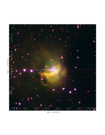
Figure 1.— The optical color composite image of Sh2-297 region made using 6724 Å [SII] image (red), 6563 Å H$\alpha$ image (green) and 5007 Å [OIII] image (blue), observed using HCT (see Section 2.1). The black square marks the position of the ionizing star HD 53623.

2. Observations and data reduction

2.1. Optical photometry

Optical photometric observations were performed using the 2 m Himalayan Chandra Telescope (HCT), Hanle (India), operated by the Indian Institute of Astrophysics, Bangalore. The telescope has Ritchey-Chretien optics with an f/9 Cassegrain focus. Both broadband and narrowband observations were performed using Himalayan Faint Object Spectrograph and Camera (HFOSC) mounted on the telescope. HFOSC has a SITe (Scientific Imaging Technologies Inc.) 2k $\times$ 4k pixels CCD, with the central region of 2k $\times$ 2k being used for imaging. With a pixel scale of 0.3${}^{{}^{\prime\prime}}$, this translates to a field of view (FoV) of $\sim$ 10${}^{{}^{\prime}}$ x 10${}^{{}^{\prime}}$. Long and short exposure observations were taken in Bessell V (600 s & 20 s) and I (300 s & 10 s) filters (centered at $\alpha_{2000}$ $\approx$ 07^h05^m13^s, $\delta_{2000}$ $\approx$ -12^o19${}^{{}^{\prime}}$03${}^{{}^{\prime\prime}}$) on 2009 October 21. [SII] (6724 Å), H$\alpha$ (6563 Å), & [OIII] (5007 Å) filter observations (centered at $\alpha_{2000}$ $\approx$ 07^h05^m17^s, $\delta_{2000}$ $\approx$ -12^o19${}^{{}^{\prime}}$18${}^{{}^{\prime\prime}}$), with an integration time of 300 s each, were done on 2010 January 18. Along with the object frames, several bias frames, twilight flat-field frames, and the standard field SA98 (Landolt, 1992) were also observed. The average seeing size ranged from $\sim$ 2${}^{{}^{\prime\prime}}$ to 3${}^{{}^{\prime\prime}}$ full width half maxima (FWHM). The standard field was used to calculate the extinction coefficients so as to calibrate our CCD systems. The astrometric calibration, with a position accuracy better than 0.3${}^{{}^{\prime\prime}}$, was done using the 2MASS sources in the field. For all the filters, frames of equal exposure time were co-added to improve the signal-to-noise ratio. Photometry was carried out only for V and I filters. Image Reduction and Analysis Facility (IRAF) data reduction package was used for the initial CCD image processing. Thereafter, using DAOPHOT II package of MIDAS, the point spread function (PSF) photometry and the photometric measurements were performed. A variable PSF was made using several uncontaminated stars in the field. Finally, the magnitudes (V and I) were calibrated in the manner outlined by Stetson (1987), with a precision better than 0.05 mag. In the present work, we have used only those sources which have magnitude errors $<$ 0.15 mag ($\sim$ 3$\sigma$).

2.2. Optical spectroscopy

The optical spectroscopic observations were carried out using HCT and the 2 m IUCAA Girawali Observatory (IGO) telescope at Girawali near Pune (India), operated by Inter University Centre for Astronomy & Astrophysics (IUCAA), Pune.

The HCT data was obtained on 2009 December 21 using HFOSC, with the help of Grism 7 (3500 to 7000 Å) - which has a resolving power of 1200 and a spectral dispersion of 1.45 Å pixel^-1. The spectrum of the star HD 53623 (catalog ) ($\alpha_{2000}$ $=$ 07^h05^m16.75^s, $\delta_{2000}$ $=$ -12^o19${}^{{}^{\prime}}$34.5${}^{{}^{\prime\prime}}$; V=7.99 mag) with an exposure time of 480 s, in addition to FeAr lamp arc spectrum (for wavelength calibration) and multiple bias frames, was obtained. The spectrophotometric standard star G91B2B (Massey et al., 1988) was also observed with an exposure time of 1200 s. Spectral reduction was carried out using “APALL” task in IRAF reduction package. Finally, the flux-calibrated spectrum was obtained (see Figure 2).

To cross-verify the weak diagnostic lines in the object spectrum from HCT, we also obtained a deeper spectrum (for 1200 s) for HD 53623 (catalog ) using IGO telescope, on 2009 November 26. The telescope has a Cassegrain focus with a focal ratio of f/10. IUCAA Faint Object Spectrograph and Camera (IFOSC), with a 2k $\times$ 2k pixel CCD array, was used for the purpose. Grism 7, with a range of 3800-6840 Å, resolving power of 1300, and a spectral dispersion of 1.49 Å pixel^-1 was used. Multiple bias frames, halogen flat-field frames, and HeNe lamp arc spectrum (for wavelength calibration) were obtained along with the object spectrum. The reduction was done using “DOSLIT” task in IRAF. No flux calibration was done for this case. Finally, the normalized spectrum was obtained (see Figure 2).

To identify the H$\alpha$ emission line stars, two grism slitless spectra (420 s each) - using Grism 5 (5200-10300 Å) and H$\alpha$ broadband filter ($\lambda=$ 6563 Å, $\triangle\lambda=$ 500 Å) - were also obtained with HCT on 2007 November 16 (centered at $\alpha_{2000}$ $\approx$ 07^h05^m23^s, $\delta_{2000}$ $\approx$ -12^o19${}^{{}^{\prime}}$00${}^{{}^{\prime\prime}}$). As a reference, for the identification of stars whose slitless spectra were obtained, two H$\alpha$ broadband filter images of the field were taken as well. Here, the first step was to average the two photometric H$\alpha$ filter images and the two slitless spectra of the region to improve their signal-to-noise ratio. The world coordinate system (wcs) coordinates were then implemented on the averaged photometric image by identifying a bright set of stars in the FoV, from the USNO catalogue, and finally synthesizing their J2000 coordinates and pixel coordinates from the image, using the generic IRAF commands “CCMAP” and “CCSETWCS”. The averaged spectrum was then analyzed in ds9 image display device, and the stars with an H$\alpha$ emission line (detectable as an enhancement over the continuum) were identified manually by careful visual inspection, with the help of photometric image of the field. 19 H$\alpha$ emission line stars were identified. The detection limit of this identification is $\sim$ 3.3 Å in terms of equivalent width, with the faintest star having a V magnitude of 20.07. Fifteen were located in our NIR FoV, and hence the NIR magnitudes for the remaining 4 were taken from 2MASS catalogue for further analysis.

Figure 2.— (a) Flux-calibrated spectrum of the central ionizing star, HD 53623, obtained with HCT (b) Normalized spectrum of HD 53623 obtained with IGO.

2.3. Near infrared observations

The region of interest, being a star forming region, has considerable nebulosity and dark cloud to the west, and hence is obscured at optical wavelengths. Moreover, we need to identify and classify the embedded YSOs which emit at longer wavelengths, hence we use NIR observations. NIR observations, centered on $\alpha_{2000}$ $\approx$ 07^h05^m11^s, $\delta_{2000}$ $\approx$ -12^o18${}^{{}^{\prime}}$51${}^{{}^{\prime\prime}}$ for the object, in $J$ ($\lambda=1.25\,\mu$m), $H$ ($\lambda=1.63\,\mu$m) and $K_{\mbox{s}}$ ($\lambda=2.14\,\mu$m) bands, were carried out on 2007 February 27 using the f/10 Cassegrain 1.4 m Infrared Survey Facility (IRSF) telescope, South Africa with SIRIUS (Simultaneous InfraRed Imager for Unbiased Survey) - a three color simultaneous camera. The camera is equipped with three 1k $\times$ 1k HgCdTe arrays, with a FoV of $\sim$ 7.8${}^{{}^{\prime}}$ $\times$ 7.8${}^{{}^{\prime}}$, and a pixel scale of 0.45${}^{{}^{\prime\prime}}$. Further information about the instrument can be found in Nagashima (1999) and Nagayama (2003). For each band, 40 frames each, centered at 9 dithered positions, were taken. The integration time for each frame was 10 s, giving a total integration time of 3600 s (9$\times$40$\times$10) in each band for the Sh2-297 (catalog ) region. The sky condition was photometric, with the average seeing size ranging from 1.35${}^{{}^{\prime\prime}}$ to 1.60${}^{{}^{\prime\prime}}$ FWHM during the observations.

The standard data reduction procedure - involving bad pixel masking, dark subtraction, flat field correction, sky subtraction, combination of dithered frames, adding wcs coordinates to the image and PSF photometry - was carried out using IRAF. Astrometric calibration was implemented using the 2MASS sources in the field. About 30-40 stars, with good profiles, were selected for calibration for each band, and an accuracy of better than $\pm$ 0.04${}^{{}^{\prime\prime}}$ was achieved for our absolute position calibration. After the initial processing, photometry was carried out on a final FoV of $\sim$ 7.5${}^{{}^{\prime}}\times$ 7.5${}^{{}^{\prime}}$. The PSF photometry was done using “ALLSTAR” algorithm of “DAOPHOT” package in IRAF. Around 11 to 13 isolated bright stars were taken to make a PSF for each band. Subsequently, the final magnitudes were calibrated using the 2MASS stars in the field, with an rms of $\sim$ 0.07 mag for all the filters. To ensure good photometric accuracy, we restricted our catalogue to sources having uncertainty $<$ 0.15 mag ($\sim$ 2$\sigma$), independent of brightness, in all the three bands. Also, it was found that the sources with $K_{\mbox{s}}$ magnitude $\leq$ 8 were saturated in our catalogue; hence their magnitudes, in all three filters, were replaced by the corresponding 2MASS values. We evaluated the completeness limits for our images by doing artificial star experiments. Stars of varying magnitudes were added to the images, and then it was determined what fraction of stars were recovered in each magnitude bin. The recovery rate was greater than 90$\%$ for magnitudes brighter than 17, 17, and 16 in $J$, $H$, and $K_{\mbox{s}}$ bands, respectively. The recovery percentage fell to 85$\%$ for $K_{\mbox{s}}$ magnitudes in 16 to 16.5 mag bin. The change in completeness limit is negligible on using the photometric error cutoff at 0.15 mag.

The final calibrated catalogue was analyzed using the CC and CM diagrams (see Section 5). For this purpose, the required magnitudes and colors were transformed into CIT (California Institute of Technology) system using the color transformation equations given on the CALTECH website. In addition to the target region, a control field centered at $\alpha_{2000}$ $\approx$ 07^h06^m20^s, $\delta_{2000}$ $\approx$ -12^o01${}^{{}^{\prime}}$40${}^{{}^{\prime\prime}}$ (about 24${}^{{}^{\prime}}$ to the north-east of our object field) was also observed. It was reduced in a similar manner as the object frames. The control field was used to assess the level of contamination from foreground sources in the target field. It was used to delineate the maximum $H-K$ color for the foreground sources, so as to identify the young stellar sources in the region - which will have a larger color by virtue of extinction and the presence of circumstellar disk which results in excess K-band emission. Figure 3 shows a false NIR color composite (J : blue, H : green, $K_{\mbox{s}}$ : red) image of Sh2-297 region, which reveals nebulosity around the central and south-eastern region, and the dark cloud towards the west.

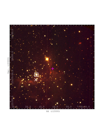
Figure 3.— Color composite made using J (blue), H (green) and $K_{\rm s}$ (red) images. White square marks the position of ionizing star HD 53623, white cross shows the position of IRAS 07029-1215, and the magenta plus marks the location of UYSO1 from Forbrich et al. (2004).

2.4. Radio continuum observations

1280 MHz observation was carried out on 2007 July 12, while that for 610 MHz on 2007 July 19, using Giant Metrewave Radio Telescope (GMRT) array. The GMRT array consists of 30 antennae, arranged in an approximately Y-shaped configuration, with each dish being 45 m in diameter. 12 antennae are located randomly in a compact 1 km$\times$1 km central square area, while the remaining 18 are located along the three radial arms (6 along each arm), each arm length being $\sim$ 14 km. The maximum baseline is $\sim$ 25 km. Further details can be found in Swarup et al. (1991). For our observations, VLA phase calibrator “0735-175” and flux calibrator “3C147” were used, at both the frequencies. The details of the observations are given in Table 1.

Table 1Details of GMRT Observations

	1280 MHz	610 MHz
Date of Obs.	2007 July 12	2007 July 19
Phase Center	$\alpha_{2000}$ = 07h05m12.30s	$\alpha_{2000}$ = 07h05m12.30s
	$\delta_{2000}$ = -12o19${}^{{}^{\prime}}$01.14${}^{{}^{\prime\prime}}$	$\delta_{2000}$ = -12o19${}^{{}^{\prime}}$01.14${}^{{}^{\prime\prime}}$
Flux Calibrator	3C147	3C147
Phase Calibrator	0735-175	0735-175
Cont. Bandwidth	16 MHz	16 MHz
Primary Beam	24${}^{{}^{\prime}}$	43${}^{{}^{\prime}}$
Resolution of maps
used for fitting	23.5${}^{{}^{\prime\prime}}\times$13.9${}^{{}^{\prime\prime}}$	23.8${}^{{}^{\prime\prime}}\times$13.6${}^{{}^{\prime\prime}}$
Peak Flux Density	19.42 mJy/beam	41.33 mJy/beam
rms noise	2.32 mJy/beam	3.24 mJy/beam
Integrated Flux Density	0.67 Jy	0.64 Jy

The radio data from GMRT was analyzed with the help of Astronomical Image Processing Software (AIPS) distributed by NRAO. The data was edited to flag the bad antenna pairs, baselines, and time ranges using the “VPLOT”, “UVFLG”, and “TVFLG” tasks. The final image was produced using a set of tasks which involved fourier inversion, cleaning (using the task “IMAGR” in AIPS), followed by a few iterations of phase-only self-calibration (till the rms convergence) to remove the effects of the atmospheric and ionospheric phase distortions.

Also, since our source is located near the Galactic plane, we had to take into account the system temperature corrections for GMRT. Since, at metre wavelengths, there is a large amount of radiation from the Galactic plane, the effective temperature of the antennae increases, which has to be corrected for. This was done by obtaining the sky temperature map of Haslam et al. (1982) at 408 MHz, and rescaling the image by a scaling factor which is just the ratio of system temperature towards the target source and the flux calibrator (here 3C147). The temperature for the source will be T${}_{\mbox{f}}$ + T${}_{\mbox{sys}}$, where T${}_{\mbox{f}}$ = T₄₀₈ $\times$(f/408)^-2.6 (using the spectral index given in Haslam et al., 1982), with T₄₀₈ being the temperature value from Haslam’s map at 408 MHz and “f” being the frequency (in MHz) for which the correction is to be calculated. T${}_{\mbox{sys}}$, the system temperature, was obtained from the National Centre for Radio Astrophysics (NCRA) website for both the frequencies. The temperature for the flux calibrator will merely be T${}_{\mbox{sys}}$, hence the scaling factor is (T${}_{\mbox{f}}$ + T${}_{\mbox{sys}}$)/T${}_{\mbox{sys}}$.

In addition, for 1420 MHz, the archival image from Very Large Array (VLA), for the observation date 1998 December 14, was also used (Project ID AF346).

Radio continuum interferometric data, at 610 MHz, 1280 MHz and 1420 MHz was used to probe the ionized gas component. The GMRT maps were convolved to a resolution of about 24${}^{{}^{\prime\prime}}\times$14${}^{{}^{\prime\prime}}$, approximately same as the VLA map. After obtaining the contour maps for all the three frequencies, the integrated flux was found by fitting a 3$\sigma$ contour level box and using the AIPS task “IMSTAT” (see Table 1). Using these radio continuum data points, the various physical parameters of the region were calculated (see Section 4.2).

3. Other available data sets

3.1. Near infrared data from 2MASS

We used the 2MASS data in the field for our photometric and astrometric calibrations. The stars were obtained using the task “IMTMC” in “WCSTOOLS” package in IRAF, for the $J$ ($\lambda=1.25\,\mu$m), $H$ ($\lambda=1.63\,\mu$m) and $K_{\mbox{s}}$ ($\lambda=2.14\,\mu$m) bands. All the sources which were obtained for calibration had a good quality flag value of “AAA” for the magnitudes. We also substituted the 2MASS magnitudes for those sources which were found to be saturated in our IRSF catalogue, i.e. those for which we had IRSF $K_{\mbox{s}}$ magnitude $\leq$ 8.

3.2. Near and mid infrared data from WISE

Wide-field Infrared Survey Explorer (WISE) surveyed the entire sky in the NIR bands at 3.4 $\mu$m (w1) and 4.6 $\mu$m (w2), and in the MIR bands at 12 $\mu$m (w3) and 22 $\mu$m (w4), with an astrometric precision better than $\sim$ 0.15${}^{{}^{\prime\prime}}$ (Wright et al., 2010). The spatial resolution was $\sim$ 6${}^{{}^{\prime\prime}}$ for the first three bands and $\sim$ 12${}^{{}^{\prime\prime}}$ for 22 $\mu$m.

Since the WISE (Preliminary Release April 2011) catalogue had many sources missing (e.g. for w1 band, only $\sim$ 35$\%$ of the sources detected in our photometry were present in the release catalogue), as could also be visually discerned, we carried out aperture photometry on the archival WISE images - for the same FoV as our IRSF NIR field - following the method described by Koenig et al. (2012). This significantly improved the number of sources detected. Photometry was done using the DAOPHOT package in IRAF; with the aperture radius, inner radius of the sky annulus, & outer radius of the sky annulus being 5${}^{{}^{\prime\prime}}$, 7.5${}^{{}^{\prime\prime}}$, & 25${}^{{}^{\prime\prime}}$ for the 3.4 & 4.6 $\mu$m bands, and 7.5${}^{{}^{\prime\prime}}$, 10${}^{{}^{\prime\prime}}$, & 25${}^{{}^{\prime\prime}}$ for the 12 $\mu$m band, respectively. The 22 $\mu$m band was not used mainly because of its low resolution, as well as the dominant nebulosity and the presence of not many point sources (12 sources were detected out of which 9 were in highly nebulous central region). The photometry for each band was calibrated with the WISE preliminary release catalogue. Care was taken not to use the objects flagged as “D” (diffraction spikes), “H” (halos from bright sources), “P” (persistent artifacts), or “O” (optical ghosts of bright sources) in the release catalogue for calibration. For the final WISE catalogue, we took only those sources which had all magnitude errors $\textless$ 0.3, to make sure that they had reliable photometry.

Our IRSF NIR catalogue was subsequently matched with the WISE catalogues within a 3${}^{{}^{\prime\prime}}$ matching radius. 187, 124, and 9 sources detected in our NIR FoV had 3.4 $\mu$m, 4.6 $\mu$m, and 12 $\mu$m counterparts, respectively. The resultant final catalogue was used to get the SEDs of various sources, and hence in constraining the manifold physical parameters like age, mass, accretion rates etc. for them (see Section 5.6). The 3.4 $\mu$m and 12 $\mu$m bands contain prominent polycyclic aromatic hydrocarbon (PAH) features at 3.3, 11.3 & 12.7 $\mu$m (Wright et al., 2010; Samal et al., 2007) in addition to the continuum emission, and hence can be used to get an idea of the photodissociation region. The 22 $\mu$m band can be used to examine the warm dust emission - the stochastic emission from small grains as well as the thermal emission from large grains (Wright et al., 2010).

4. Morphology of the region

4.1. The ionizing source

The ionizing source of Sh2-297 (catalog ) region is the star HD 53623 (catalog ), associated with the reflection nebula CMa R1 (catalog ) (Van Den Bergh, 1966). Clariá (1974) and Houk & Smith-Moore (1988) estimated the spectral type of this source as B1Vn and B1II/III, respectively, using objective-prism plates from Michigan Curtis-Schmidt telescope, CTIO. Herbst et al. (1978) have proposed the spectral type as B0.5 IV-V using spectrogram analysis. Here we use the optical spectroscopic data to find out the spectral type of this source. The reduced spectra from HCT and IGO, for the wavelength range 3950 to 4750 Å, have been shown in Figure 2. The spectra were analyzed with the help of Walborn spectra catalogue (Walborn & Fitzpatrick, 1990). The absence of He ii lines at 4200 & 4541 Å, and low strength at 4686 Å suggest that the star does not belong to O-type spectral class. The most prominent lines in our spectra are the He i lines at 4009, 4026, 4144, 4387, 4471, and 4713 Å. The Balmer lines at 3970 Å (H$\varepsilon$), 4102 Å (H$\delta$), and 4341 Å (H$\gamma$) are clearly seen too. We also see C iii + O ii blend at 4070 and 4650 Å. Weak Si iv line at 4116 Å, weak O ii lines at 4415-4417 Å, and absence of Si iii lines indicate that the star most probably does not belong to giant luminosity classes. The preponderance of neutral helium lines and the comparison with the standard Walborn catalogue suggest a most likely spectral type of B0V/B0.5V for the star. Tjin A Djie et al. (2001) have suggested, using H$\alpha$ emission study, that this source does not contain any circumstellar disk, most probably due to photoevaporation by UV photons or due to influence of some supernova in the nearby region.

4.2. Physical properties of the region

High resolution studies are important as they help us in understanding the structure of a region. Sh2-297 (catalog ) has been observed with very coarse resolutions in previous radio surveys, which makes it harder to recognize the subtler features in the radio emission. For example, the survey by Felli & Churchwell (1972) observed 168 optically identified H ii regions at 1400 MHz, including Sh2-297 (catalog ), with a spatial resolution of 10${}^{{}^{\prime}}$. Similar observations were carried out by Pyatunina (1980) for wavelengths ranging from 2 to 11 cm, with resolutions of $\sim$ 1${}^{{}^{\prime}}-$4.3${}^{{}^{\prime}}$. At larger frequencies (10 GHz), the CMa R1 region was observed by Nakano et al. (1984) with a resolution of 2.7${}^{{}^{\prime}}$. Fich (1993), in a VLA survey, observed the region at 1.4 GHz with 43${}^{{}^{\prime\prime}}$ resolution. Figure 4 shows GMRT high resolution greyscale contour maps, for 610 MHz ($\sim$ 10${}^{{}^{\prime\prime}}\times$ 5${}^{{}^{\prime\prime}}$) and 1280 MHz ($\sim$ 7${}^{{}^{\prime\prime}}\times$ 6${}^{{}^{\prime\prime}}$), of Sh2-297 (catalog ) H ii region. The intricate morphology of Sh2-297 (catalog ) - showing the complex structures and the clumpy nature - can very well be discerned on examination. The radio emission morphology from our observation as well as the location of H ii region at the tip of the molecular cloud (see Section 4.3) suggest that the ionized gas is possibly undergoing a champagne flow (also known as blister region) (Tenorio Tagle et al., 1979; Alloin & Tenorio Tagle, 1979), with the extended emission towards the east and the head of the ionized champagne flow located to the west towards LDN1657A (catalog ) (see Section 6).

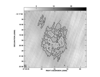
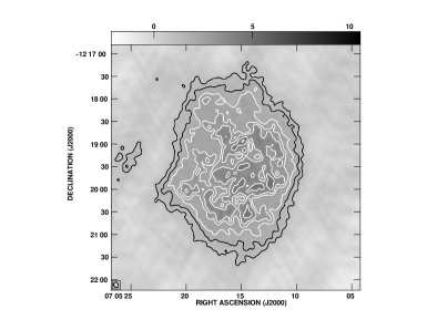
Figure 4.— ($upper\,panel$) High resolution GMRT radio map for 610 MHz ($\sim$ 10${}^{{}^{\prime\prime}}\times$5${}^{{}^{\prime\prime}}$). Contours have been drawn at 12, 16, 20, 24, & 30 % of the peak flux (28.30 mJy/beam). ($lower\,panel$) High resolution GMRT map for 1280 MHz ($\sim$ 7${}^{{}^{\prime\prime}}\times$ 6${}^{{}^{\prime\prime}}$). Contours have been drawn at 10, 15, 20, 25, 30, 40, & 50 % of the peak flux (10.47 mJy/beam).

The radio continuum observations of the region using GMRT, and archival data from VLA, were used to calculate the various physical parameters which characterize an H ii region (emission measure, electron density, strömgren radius, and dynamical timescale). Assuming a spherically symmetric and homogeneous ionized region, the model of Mezger & Henderson (1967) for free-free emission was used. According to this, the flux density arising due to the region is given by the following (adapted from Mezger et al., 1967, Equations 1 and 3) :

$$S_{\nu}=3.07\times 10^{-2}T_{e}\nu^{2}\Omega(1-e^{-\tau(\nu)})$$ (1)

$$\tau(\nu)=1.643\times 10^{5}aT_{e}^{-1.35}\nu^{-2.1}n_{e}^{2}l$$ (2)

where, $S_{\nu}$ is the integrated flux density in Jansky (Jy), $T_{e}$ is the electron temperature of the ionized core in K, $\nu$ is the frequency in MHz, $n_{e}$ is the electron density in cm^-3, $l$ is the extent of the ionized region in pc, $\tau$ is the optical depth, $a$ is the correction factor, and $\Omega$ is the solid angle subtended by the beam in steradian (approximating the beam with a Gaussian, the beam solid angle is given by $\Omega=1.133\times\theta_{maj}\times\theta_{min}$, where $\theta_{maj}$ and $\theta_{min}$ are major and minor half power beam widths). The factor $n_{e}^{2}l$ denotes the emission measure (in cm^-6 pc), a measure of optical depth of the medium. For our calculations, we set the value of $a$ as 0.99 (obtained from Mezger & Henderson, 1967, Table 6), and that of $T_{e}$ to 10000 K - applicable to classical H ii regions (Stahler & Palla, 2004). Thereafter, treating the emission measure as a free parameter and using the three data points (flux density vs. frequency) from the three maps, a non-linear regression was implemented, following a procedure similar to Vig et al. (2006) (see Figure 5), which yielded the value of the free parameter (emission measure), for the best fit, as 9.15 $\pm$ 0.56 $\times$ 10⁵ cm^-6 pc. The extent of this extended H ii region is $\sim$ 5${}^{{}^{\prime}}$, as obtained from the VLA image. At a distance of 1.1 kpc, this translates to an extent of 1.6 pc. From the emission measure and the extent, the electron density is obtained to be 756 $\pm$ 46 cm^-3. The low values of the emission measure and the electron density reinforce the fact that this is a classical, and thus, evolved H ii region (see Stahler & Palla, 2004).

Figure 5.— Observed and fitted flux density (solid line) for the H ii region. Filled circles and triangle represent GMRT & VLA data, respectively. The flux densities were calculated for an approximately same resolution of $\sim$ 24${}^{{}^{\prime\prime}}\times$14${}^{{}^{\prime\prime}}$.

Further, assuming a homogeneous and spherically symmetric nature for the H ii region, the luminosity of the Lyman continuum photons (in photons s^-1) from the central ionizing source is given by (Moran, 1983, Equation 5) :

$$S_{*}=8\times 10^{43}\left(\frac{S_{\nu}}{mJy}\right)\left(\frac{T_{e}}{10^{4}K}\right)^{-0.45}\left(\frac{D}{kpc}\right)^{2}\left(\frac{\nu}{GHz}\right)^{0.1}$$ (3)

where $S_{\nu}$ is the integrated flux density in mJy from the contour map, $D$ is the distance in kiloparsec, $T_{e}$ is the electron temperature, and $\nu$ is the frequency in GHz for which the luminosity is to be calculated. For our calculations, we used the 1420 MHz flux value (0.76 Jy). $D$ was taken to be 1.1 kpc and $T_{e}$ as 10⁴ K. The value for $S_{*}$ was determined to be 7.62$\times$10⁴⁶ photons s^-1 (hence $\log S_{*}$ is 46.88). Bonatto & Bica (2009) have estimated the main sequence (MS) age of HD 53623 (catalog ) as 5 $\pm$ 3 Myr, therefore assuming a luminosity class V for it, a comparison of $\log S_{*}$ with Panagia (1973, Table II) yields the spectral type as B0, in agreement with our optical spectroscopic analysis. The lower value of our calculated luminosity ($\log S_{*}$) as compared to the theoretical value (47.63) from Panagia (1973) could be because of absorption of photons by dust in the region.

As the central massive star ionizes the ambient medium around it, the ionization front moves outwards, and the whole H ii region expands till an equilibrium is reached between the number of ionizations and recombinations. The underlying assumption here is that the ambient medium has homogeneous density and temperature. Using the formulation given by Strömgren (1939), the radius of the H ii region at this point - called Strömgren radius - is given by :

$$R_{s}=\left(\frac{3S_{Lyman}}{4\pi n_{o}^{2}\beta_{2}}\right)^{1/3}$$ (4)

where $R_{s}$ is the Strömgren radius (in cm), $n_{o}$ is the initial ambient density (in cm^-3), and $\beta_{2}$ is the total recombination coefficient to the first excited state of hydrogen. The value of $\beta_{2}$, for a $T_{e}$ of 10⁴ K, is taken to be 2.6$\times$10^-13 cm³ s^-1 (Stahler & Palla, 2004). We estimated the initial ambient density as follows (similar to Strömgren, 1939). From the luminosity calculations for Lyman continuum photons, we have obtained a calculated value of 7.62$\times$10⁴⁶ photons s^-1 ($S_{*}$), which is about 18% of the theoretical output of 4.27$\times$10⁴⁷ photons s^-1 (Panagia, 1973). This implies that $n_{e}=0.18n_{o}$, hence yielding $n_{o}$ as 4202 $\pm$ 253 cm^-3, using the above calculated value of the electron density. Using these values for $S_{*}$ and $n_{o}$, the strömgren radius turns out to be 0.051 $\pm$ 0.002 pc.

As the gas expands, it sends a shock front into the neutral medium. This shock front precedes the ionization front. At this stage, the radius of the H ii region is given by (Spitzer, 1978):

$$R(t)=R_{s}\left(1+\frac{7c_{II}t}{4R_{s}}\right)^{4/7}$$ (5)

where $R(t)$ is the extent of the H ii region at time $t$, and $c_{II}$ is the speed of sound, taken to be 11$\times$10⁵ cm s^-1 (Stahler & Palla, 2004). Using the current extent of 1.6 pc as the value of $R(t)$, and the above calculated value of $R_{s}$ in this equation, we obtain the value of $t$, referred to as the dynamical timescale, as 1.07 $\pm$ 0.31 Myr.

It should be noted that, to calculate $R_{s}$ and $t$, we have estimated $n_{o}$ (4202 $\pm$ 253 cm^-3) assuming a luminosity class V for the massive star, and that only part of the radio flux is used for ionization. Also, we have used the current value of electron density. However, at the beginning of massive star formation, $n_{o}$ could be of the order of 10⁴-10⁵ cm^-3 (Ward-Thompson & Whitworth, 2011). Besides, the expansion velocity decreases with time. Hence, the electron density and the dynamical timescale calculated here should be treated as conservative lower limits.

4.3. Infrared and submillimetre structures

Figure 6 shows the ¹²CO(J=3-2) image of the region (public processed data for observation date 2011 February 20, Project ID: M11AH48A) from James Clerk Maxwell Telescope (JCMT). The MSX 8.28 $\mu$m contours (in yellow), SCUBA 850 $\mu$m contours (in red) (Di Francesco et al., 2008), and the 1280 MHz radio contours from GMRT (in white) are overlaid. The MSX A band ($\lambda=$ 8.28 $\mu$m; containing PAH features at 7.7 & 8.7 $\mu$m besides continuum emission) contours give an idea of the PAH distribution in the region (see e.g. Deharveng et al., 2005). ¹²CO(J=3-2) traces the molecular hydrogen, while SCUBA 850 $\mu$m traces the cold dust. As can be seen from the figure, there is a clear correlation between the ionized gas and 850 $\mu$m contours in Sh2-297 central region. The ¹²CO image shows a D-shaped ring to the south of HD 53623 (catalog ), which is also traced by the MSX A band contours, and is faintly visible in narrowband H₂ S(1) image of Forbrich et al. (2009, see their Figure 1). This is probably due to the sweeping up and piling of material from the expanding H ii region, and as such it is a potential site for future triggered star formation by collect-and-collapse process. Also noticeable is the fact that, towards the west, PAH extends roughly upto the interface of the H ii region and LDN1657A.

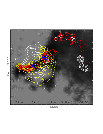
Figure 6.— The ¹²CO(J=3-2) image (log greyscale with intensity range -1 to 30 K km s^-1) of the region from JCMT, overlaid with MSX 8.28 $\mu$m contours (yellow) showing the PAH distribution, SCUBA 850 $\mu$m contours (red) which trace the cold dust, and 1280 MHz radio continuum contours (white) indicating the ionized gas. The CO image reveals a maximum column density of 87.28 K km s^-1. MSX and SCUBA contours have been plotted at 10, 15, 20, 25, 30, 40 & 50 % of their peak values, which are 49.666 mW/m²-Sr and 1.619 Jy/beam, respectively. Radio contours ($\sim$ 25${}^{{}^{\prime\prime}}$ resolution) have been plotted at 3, 6, 9, 15, and 21$\sigma$ ($\sigma$ denotes the rms noise, which is 1.03 mJy/beam) levels. The blue square marks the ionizing star HD 53623, blue plus symbol marks the position of UYSO1 from Forbrich et al. (2004), blue circle marks the position of C₂H peak from Beuther et al. (2008), blue cross denotes IRAS 07029-1215, and the sources from Linz et al. (2010) have been labelled and marked in white circles.

The WISE w4 band which traces the warm dust and thermal emission from protostars (not shown here), and SCUBA data show that the warm and cold dust extend well beyond the H ii region, and also towards the cold, dark cloud LDN1657A (catalog ). The gas and dust correlation is evident in the FIR IRAS 100 $\mu$m wavelength as well (Gregorio-Hetem, 2008). The nebula around the star HD 53623 (catalog ) shows a high level of FIR emission. Beuther et al. (2008) found a C₂H peak near IRAS 07029-1215 (catalog ), coinciding with UYSO1 (see Figure 6), thereby indicating that this is a young star forming region (Vasyunina et al., 2011). Kim et al. (2004) have probed the dense molecular gas using the optically thin $J=1-0$ transition of ¹³CO. One of the peaks is at $l=225.47^{o}$, $b=-2.80^{o}$ (outside the range of Figure 6), showing the presence of dense gas further towards the south-west of Sh2-297 (catalog ) as well.

5. Stellar population in the region

5.1. NIR color-color diagram

The NIR CC diagram for the IRSF sources, showing the $J-H$ vs. $H-K$ colors, is given in Figure 7. The thick red line denotes the locus of MS stars, the magenta line shows the locus of giant stars while the dotted black straight line is the locus of Classical T Tauri Stars (CTTS). The loci for the MS and giants were taken from Bessell & Brett (1988) while those for the CTTS from Meyer et al. (1997). The three parallel dashed and slanted lines are the reddening vectors ($A_{J}/A_{V}=0.265$, $A_{H}/A_{V}=0.155$ and $A_{K}/A_{V}=0.090$) for the CIT system from Cohen et al. (1981). The crosses mark every 5 mag increase in $A_{V}$. We converted the colors from 2MASS to CIT system, as was discussed in Section 2.3.

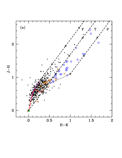
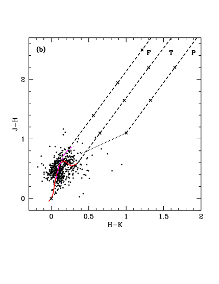
Figure 7.— (a) NIR CC diagram for the object field. The red curve shows the MS locus and the magenta curve shows the locus of giant stars. The locus of CTTS has been shown by a black dotted line. The three parallel and slanted lines are the reddening vectors, with crosses on them marking an interval of $A_{V}$= 5 mag. Blue circles denote the Class II-type sources, orange crosses the H$\alpha$ emission line stars, and the green square the central ionizing star. (b) The CC diagram for the control field.

We used the CC diagram to identify and study the nature of YSOs in the region. Since young sources have a significant infrared excess, which in turn can be used to identify them, we divided our CC diagram into three regions - F, T and P (similar to Ojha et al., 2004b, c). The region “F” mostly contains the field stars and Class III sources (weak-line T Tauri stars). The region “T” contains the CTTS (Lada & Adams, 1992), Class II objects with large NIR excesses, and reddened early type ZAMS (Zero Age Main Sequence) stars with K-band excess emission. The “P” zone sources are most likely Class I objects (protostar-like objects) with circumstellar envelopes. The NIR CC diagram is likely to be contaminated by the foreground and background field stars. To assess this, we also plotted the CC diagram for the control field (Figure 7). On comparison, we find that almost all our control field sources are confined to the left of the middle reddening vector, and a few which are to its right are below the CTT locus. Thus, the “T” and “P” regions of the object field are mostly uncontaminated by the field stars, and hence the sources in these regions can be assumed to be YSOs.

As there is considerable nebulosity in the region, it must be kept in mind that there could be dust knots emitting at near and mid infrared wavelengths. These could be mistakenly identified as Class I/II sources in the CC diagram. Hence, this CC diagram has its limitations when it comes to the identification of the YSOs, and the information from it is only complementary to other techniques like spectroscopy, to understand the nature of objects. The spatial distribution of the YSOs identified was used to pin down the star formation process going on in this region (see Section 5.7).

5.2. NIR color-magnitude diagram

The NIR CM diagrams, $K/(H-K)$, of the region and the control field are shown in Figure 8. The nearly vertical solid lines are the loci of ZAMS reddened by $A_{V}=0,\,15,\,30$ and $45$ mag. The slanting lines are the reddening vectors for the corresponding spectral types. A comparison of the object field and the control field CM diagrams shows an apparent separation between the stellar sources at around $H-K\sim$ 0.6. Our control field shows almost all sources having $H-K<0.6$, thereby indicating that sources with $H-K<0.6$ are most likely the foreground stars. The sources lying to the right of the $H-K=0.6$ cut-off line (shown with a dashed vertical line in Figure 8) have an excess emission in the K-band and can thus reasonably be assumed to be young protostars. A CC diagram ($K_{\mbox{s}}-3.4$/$3.4-4.6$, Koenig et al., 2012) for the red sources which had WISE counterparts (not shown here) showed their location in the diagram to be consistent with the location of Class I sources. The central ionizing star has been marked with a green square on this diagram. The NIR CM diagram indicates a B1 spectral type for the ionizing source, which is within one sub-class of that estimated from the optical spectroscopy and radio continuum observations. However, a spectral type derived from just two data points ($H$ and $K$) is not very reliable because of uncertainty in distance determination. It just serves to give an idea of the spectral type, the spectrum analysis being canonical in this respect.

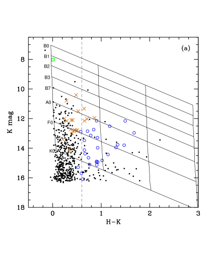
Figure 8.— (a) NIR CM diagram for our object field. The nearly vertical solid lines are the loci of ZAMS stars reddened by $A_{V}$=0, 15, 30, & 45 mag. The parallel, slanting lines denote the reddening vectors. Blue circles denote the Class II-like objects, orange crosses the H$\alpha$ emission line stars, and the green square the central ionizing star. The $H-K$ cut-off at 0.6 has been marked with a dashed vertical line. (b) CM diagram for the control field.

We estimated the extragalactic contamination (extincted or faint background galaxies) in our sample of NIR excess sources. We assume that the extragalactic sources can be seen through maximum extinction, which for our case is A${}_{V}\sim$ 25 mag (A${}_{K}\sim$ 2.25 mag) (see Section 5.3). Accounting for the interstellar extinction and converting the K_S magnitude to AB system (since K_S counts are tabulated in AB photometric system in Keenan et al. (2010)), the total number of galaxy counts in our NIR region, i.e. $\sim$ 56.25 arcmin², turns out to be 6 $\pm$ 2 down to our faintest detected magnitude of $\sim$ 17 in the K_S band.

A list of all the YSOs, with their respective magnitudes in optical and IR, has been given in Table 2. 97 YSOs were analyzed in total, with 93 of them in our NIR FoV of $\sim$ 7.5${}^{{}^{\prime}}\times$ 7.5${}^{{}^{\prime}}$, and 4 H$\alpha$ emission line stars outside this FoV (but considered for analysis nevertheless). Out of the 93 YSOs, 15 are H$\alpha$ emission line stars detected using grism slitless spectroscopy with a V limiting magnitude of 20.07, 76 are NIR YSOs (26 Class II-type sources $+$ 50 red sources with $H-K>0.6$) with a limiting $K_{\mbox{s}}$ magnitude of $\sim$ 17, and 2 are LDN1657A-2 and LDN1657A-3 sources from Linz et al. (2010) (only LDN1657A-3 was detected in NIR). Class II-like and $H-K>0.6$ sources which were also detected as H$\alpha$ emission line sources were classified as H$\alpha$ emission line sources. The $H-K>0.6$ sources which overlapped with Class II-like sources were classified as Class II-like sources.

Table 2Optical & infrared magnitudes for the YSOs

Table 2 has been given at the end of the paper

5.3. Extinction in the region

The average extinction in the region was calculated using the CC diagram as well as the extinction map of the region.

To calculate the average reddening using the CC diagram, we used the sources in the “F” and “T” zones of our diagram. The sources in the “T” region were dereddened to the CTT locus, while the sources in the “F” region were dereddened to the MS locus which was approximated by a straight line asymptote. This gives the color-excess for each source. Subsequently, the reddening laws of Cohen et al. (1981) were followed to calculate the $A_{V}$ for each source. Finally, we fit the set of $A_{V}$ values (ranging from $\sim$ 0.02 to 16 mag) obtained for each of the sources, with a normal distribution. The mean of this distribution was found to be 2.70 mag.

The average visual extinction for the region was also found by making an extinction map (“NICE” method, Lada et al., 1994; Kainulainen et al., 2007). To do this, we first obtained the intrinsic $H-K$ color from the control field. Thereafter, the color-excess, E($H-K$), and then $A_{V}$ for each of the sources in our catalog was calculated. The color-excess is related to visual extinction by : E($H-K$) = 0.065$\times$ $A_{V}$, which can be calculated from the reddening laws. $A_{V}$ values ranged from 0$-$25 mag, as we took all sources with at least H and K magnitudes, and thereby even redder ones (undetected in J), here. Subsequently, the extinction map was made, where the extinction at each pixel was calculated by a weighted Gaussian mean around it. For our case, we took a Gaussian with an FWHM of 1${}^{{}^{\prime}}$. Finally, the mean pixel value for our map was calculated using the task “IMSTAT” in IRAF, which gave us an average visual extinction of 2.69 mag.

Hence, we find similar $A_{V}$ values from both the methods. We used 2.70 mag as our value for $A_{V}$ in the optical CM diagram to estimate the mass and age of the YSOs (see Section 5.4). It gives the mean extinction of the field. However, owing to the nebulosity in the central region and the presence of dark cloud to the west (see Section 5.7), individual extinction for the sources will vary depending on their location.

5.4. Optical color-magnitude diagram

Figure 9 shows the V/V-I CM diagram for the YSOs in the region. Here, H$\alpha$ emission line sources have been shown in orange crosses, Class II-like sources in blue circles, and sources with $H-K>0.6$ have been represented by red circles. Most of the sources detected at optical wavelengths are H$\alpha$ emission line sources, with only three Class II-like sources and one source with $H-K>0.6$. This is expected as H$\alpha$ emission line sources are the most evolved YSOs in the field. In Figure 9, the isochrone for 2 Myr for solar metallicity by Girardi et al. (2002), and pre-main sequence (PMS) isochrones for 0.1 to 5 Myr from Siess et al. (2000) have been overlaid. The isochrones were corrected for distance (1.1 kpc) and reddening ($A_{V}$ = 2.70 mag; see Section 5.3). The figure also shows the evolutionary tracks for masses ranging from 0.3 to 3 M_⊙ from Siess et al. (2000).

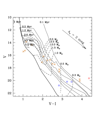
Figure 9.— Optical CM diagram showing H$\alpha$ emission line stars (orange crosses), Class II-type objects (blue circles), and $H-K>0.6$ source (red circle). The thick solid line is the 2 Myr isochrone by Girardi et al. (2002), while the thinner solid lines are PMS isochrones for different ages by Siess et al. (2000). Dashed lines are evolutionary tracks for different masses by Siess et al. (2000). The isochrones have been corrected for distance (1.1 kpc) and reddening ($A_{V}$ = 2.70 mag). The arrow shows the reddening vector for $A_{V}$ = 3 mag.

We can see that most of the YSOs lie in the age range of 0.5 to 2 Myr, with the mean age $\sim$ 1 Myr. The mass range mostly varies from 0.3 to $\sim$ 2 M_⊙, with a few outliers mainly being the H$\alpha$ emission line sources. The PMS star to the right of 0.1 Myr isochrone is likely to be a highly extincted source. It should be noted that variable extinction along the line of sight and variability could be the reason behind the age spread in our figure. Similar age spreads have been noted in other star-forming regions (Jose et al., 2008; Sharma et al., 2007).

5.5. Mass spectrum of the stellar sources

The excess K-band emission can make the YSOs appear luminous and hence the $K/H-K$ CM diagram is not appropriate for mass estimation. We therefore choose the $J/J-H$ CM diagram to minimize the effect of this excess emission which would lead to an over estimation of mass. Figure 10 shows the required CM diagram, with the Class II-like sources detected from the CC diagram (in blue circles), sources with $H-K>0.6$ (in red circles), and sources with H$\alpha$ emission line (in orange crosses). The ionizing star has also been shown with a green square. The larger statistics here as opposed to the optical CM diagram is due to the young nature of the sources, which emit at longer wavelengths. From the optical CM diagram, we found that the average age of the YSOs was about 1 Myr. Also, the dynamical age of this H ii region from radio results is 1.07 $\pm$ 0.31 Myr (see Section 4.2). Hence, we use the isochrone for 1 Myr (black solid line) from Siess et al. (2000) for our analysis. The slanting dotted lines show the reddening vectors for different masses.

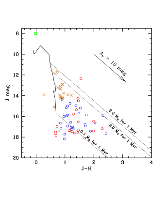
Figure 10.— J/J-H CM diagram for the YSOs. Blue circles denote the Class II-type sources, while red circles denote those with $H-K>0.6$. The H$\alpha$ emission line stars have been represented by orange crosses. The central ionizing star has been marked by a green square. The PMS isochrone for 1 Myr (solid line) from Siess et al. (2000) has been shown. The isochrone was corrected for a distance of 1.1 kpc. The slanted lines show the reddening vectors for different masses.

We can see from the 1 Myr reddening vectors, that most of the H$\alpha$ emission line objects and Class II-like sources lie between 0.1 to 2 M_⊙, though a few outliers seem to be much more massive, of the order of $\sim$ 3 M_⊙. Most $H-K>0.6$ sources have masses less than 2 M_⊙. It is noteworthy that our mass range is consistent with the mass range derived from the optical CM diagram (Section 5.4), with the H$\alpha$ emission line stars being towards the massive end. As can clearly be seen, the YSOs with the assumed age, have widely varying colors. This is probably an indication of variable extinction, weak contribution of excess emission in J and H bands, and sources being in different evolutionary stages. It should be noted that mass estimations from infrared CM diagrams are prone to systematic errors (Hillenbrand et al., 2008) due to possible use of different PMS evolutionary models, and reliance on uncertain age and distance. Another error source could be the presence of binaries, which will brighten a star - thus changing the mass and age estimates.

5.6. Spectral energy distribution

So far, we have identified the YSOs with the help of NIR CC and CM diagrams, and the H$\alpha$ emission line stars. To get an idea about the physical parameters of these sources, we modelled the SEDs using the grid of models and fitting tools of Robitaille et al. (2006, 2007).

The basic model assumes three components of any source : a PMS central star, a surrounding flared accretion disk, and a rotationally flattened envelope with cavities carved out by a bipolar outflow. Different models are computed for a suitably large parameter space - containing manifold combinations of the above mentioned components - using a Monte Carlo based radiation transfer code (Whitney et al., 2003a, b). SED fitting for different sources is not unique and the number of models for each source can only be constrained by having more data points from multiwavelength observations. To reduce error due to the uncertainties which result from very few data points, we modelled only those sources for which we had WISE data and at least five data points. The input parameters were distance range (taken to be 0.9$-$1.3 pc), and A_V (taken as 1.1$-$25 mag). The lower limit was chosen to be 1.1 mag (from the calculation of Bonatto & Bica (2009) for BDSB 96 (catalog )) as the YSOs should have an extinction which is more than the visual absorption for the region. The upper limit was chosen as 25 mag because the highest individual A_V values from color-excess calculations using NICE method (Section 5.3) were around this value. The SED fitting tool of Robitaille et al. (2007) gives a set of well constrained values for each parameter, rather than the values for only the best fit for SED. Following a similar method as Robitaille et al. (2007), we considered only those fits to constrain the physical parameters for which we had

$$\chi^{2}-\chi_{min}^{2}<3\,\mbox{(per data point)},$$ (6)

where $\chi^{2}$ is measure of goodness of fit for each model (see Figure 11). The final values were subsequently obtained using the models which satisfied Equation 6 and finding a weighted mean value for each parameter, with the weight being the inverse square of $\chi^{2}$ for each model respectively. For some of the sources, the errors for a few parameters are large because we are dealing with a large parameter space, while we have only a few data points to fit the models. The results from our SED modelling are given in Table 3. The physical parameters listed are stellar mass ($M_{\odot}$), stellar age ($t_{*}$), temperature ($T$), disk accretion rate ($\dot{M}_{disk}$), foreground visual extinction ($A_{V}$), and the $\chi^{2}_{min}$ per data point of the best fit.

Table 3SED results for the YSOs

ID	RA	Dec.	Mass	$\log t_{*}$	$\log T$	$\log\dot{M}_{disk}$	$A_{V}$	$\chi_{min}^{2}$
	(J2000)	(J2000)	(M⊙)	(yr)	(K)	(M⊙ yr-1)	(mag)
Sources from Linz et al. (2010)
1	07:04:58.030	-12:16:50.80	0.21 $\pm$ 0.39	3.37 $\pm$ 0.46	3.46 $\pm$ 0.07	-6.82 $\pm$ 0.55	16.23 $\pm$ 7.82	4.36
2	07:05:00.665	-12:16:45.13	1.27 $\pm$ 1.49	5.32 $\pm$ 0.39	3.61 $\pm$ 0.10	-7.71 $\pm$ 1.85	10.56 $\pm$ 4.20	1.89
Sources with $H-K>0.6$
19	07:05:00.919	-12:15:42.37	2.44 $\pm$ 1.00	5.43 $\pm$ 0.44	3.67 $\pm$ 0.05	-9.15 $\pm$ 1.97	7.27 $\pm$ 1.14	1.40
45	07:05:10.395	-12:19:25.70	2.91 $\pm$ 1.38	4.55 $\pm$ 1.27	3.81 $\pm$ 0.27	-6.35 $\pm$ 1.45	1.89 $\pm$ 0.78	8.28
49	07:05:13.678	-12:19:51.96	1.14 $\pm$ 0.72	5.05 $\pm$ 0.38	3.61 $\pm$ 0.03	-8.18 $\pm$ 1.11	2.90 $\pm$ 1.83	1.20
Class II-type sources
53	07:04:56.673	-12:16:12.77	0.97 $\pm$ 0.82	5.21 $\pm$ 0.37	3.60 $\pm$ 0.03	-8.74 $\pm$ 1.20	2.22 $\pm$ 1.16	3.23
54	07:04:57.964	-12:17:13.85	0.19 $\pm$ 0.22	5.90 $\pm$ 0.48	3.49 $\pm$ 0.03	-10.05 $\pm$ 1.46	3.94 $\pm$ 0.88	1.45
58	07:05:01.230	-12:19:03.69	1.28 $\pm$ 0.90	5.15 $\pm$ 0.51	3.62 $\pm$ 0.04	-9.01 $\pm$ 1.41	2.98 $\pm$ 1.32	3.34
64	07:05:08.269	-12:19:15.83	3.62 $\pm$ 2.24	5.37 $\pm$ 1.20	3.87 $\pm$ 0.30	-8.82 $\pm$ 2.73	15.93 $\pm$ 5.87	0.34
66	07:05:09.197	-12:19:00.00	0.86 $\pm$ 0.74	4.63 $\pm$ 0.72	3.59 $\pm$ 0.09	-7.88 $\pm$ 1.20	4.72 $\pm$ 2.26	1.64
69	07:05:11.424	-12:19:24.36	0.86 $\pm$ 0.71	4.72 $\pm$ 0.65	3.59 $\pm$ 0.08	-7.98 $\pm$ 1.15	4.45 $\pm$ 1.95	1.50
70	07:05:11.541	-12:18:11.39	1.32 $\pm$ 1.35	4.43 $\pm$ 0.79	3.60 $\pm$ 0.06	-7.93 $\pm$ 1.12	3.07 $\pm$ 1.37	2.21
72	07:05:11.774	-12:16:24.01	1.00 $\pm$ 0.80	5.24 $\pm$ 0.58	3.64 $\pm$ 0.13	-8.56 $\pm$ 1.45	2.71 $\pm$ 1.52	2.13
73	07:05:14.495	-12:20:47.57	0.53 $\pm$ 0.79	4.93 $\pm$ 0.89	3.52 $\pm$ 0.14	-8.76 $\pm$ 1.21	2.45 $\pm$ 1.19	0.03
75	07:05:15.324	-12:20:02.05	0.84 $\pm$ 1.09	4.42 $\pm$ 0.90	3.58 $\pm$ 0.15	-7.45 $\pm$ 1.23	2.60 $\pm$ 1.92	2.15
76	07:05:17.419	-12:18:58.69	0.81 $\pm$ 1.19	4.85 $\pm$ 1.15	3.56 $\pm$ 0.22	-8.20 $\pm$ 1.42	2.21 $\pm$ 1.01	0.04
H$\alpha$ emission line sources
79	07:05:06.330	-12:15:36.38	2.27 $\pm$ 0.67	6.63 $\pm$ 0.36	3.85 $\pm$ 0.15	-9.95 $\pm$ 1.95	5.11 $\pm$ 1.05	1.91
80	07:05:09.652	-12:19:56.32	0.89 $\pm$ 1.18	4.60 $\pm$ 0.82	3.58 $\pm$ 0.06	-7.90 $\pm$ 0.98	3.24 $\pm$ 1.59	1.15
82	07:05:12.292	-12:18:38.27	0.94 $\pm$ 0.92	5.68 $\pm$ 0.30	3.61 $\pm$ 0.04	-8.76 $\pm$ 1.15	1.46 $\pm$ 0.52	1.52
86	07:05:17.904	-12:15:40.26	4.60 $\pm$ 1.03	5.61 $\pm$ 0.07	3.78 $\pm$ 0.09	-7.48 $\pm$ 1.00	2.01 $\pm$ 0.60	2.62
87	07:05:18.494	-12:15:09.22	2.30 $\pm$ 0.72	6.04 $\pm$ 0.58	3.79 $\pm$ 0.17	-9.08 $\pm$ 1.49	2.31 $\pm$ 1.05	0.54
88	07:05:19.389	-12:20:28.71	2.51 $\pm$ 0.81	6.55 $\pm$ 0.31	3.82 $\pm$ 0.16	-9.41 $\pm$ 2.01	2.23 $\pm$ 0.92	0.24
89	07:05:19.592	-12:17:31.48	2.33 $\pm$ 0.86	5.58 $\pm$ 0.42	3.67 $\pm$ 0.05	-9.61 $\pm$ 1.32	2.12 $\pm$ 0.58	2.68
90	07:05:20.068	-12:19:12.59	3.93 $\pm$ 0.15	6.63 $\pm$ 0.13	4.15 $\pm$ 0.01	-12.90 $\pm$ 0.60	3.83 $\pm$ 0.21	1.27
91	07:05:20.728	-12:21:42.69	2.64 $\pm$ 0.78	5.57 $\pm$ 0.31	3.68 $\pm$ 0.05	-9.15 $\pm$ 1.64	1.91 $\pm$ 0.66	1.04
92	07:05:21.912	-12:19:07.19	0.26 $\pm$ 0.18	5.83 $\pm$ 0.29	3.51 $\pm$ 0.02	-10.70 $\pm$ 1.64	1.34 $\pm$ 0.34	2.61
93	07:05:22.359	-12:17:18.63	1.07 $\pm$ 0.88	6.14 $\pm$ 0.45	3.62 $\pm$ 0.06	-9.20 $\pm$ 1.18	2.06 $\pm$ 1.00	1.25
H$\alpha$ emission line sources outside NIR FoV
96	07:05:23.669	-12:22:36.08	1.69 $\pm$ 0.64	6.22 $\pm$ 0.38	3.71 $\pm$ 0.13	-9.96 $\pm$ 1.58	2.46 $\pm$ 1.11	1.64

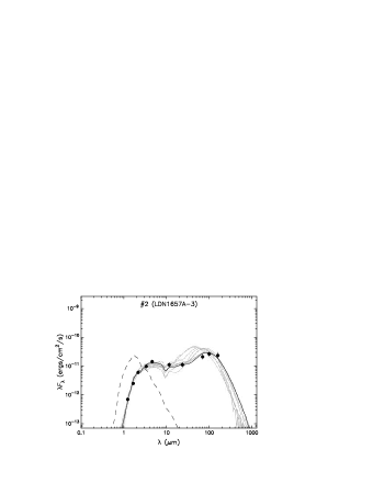
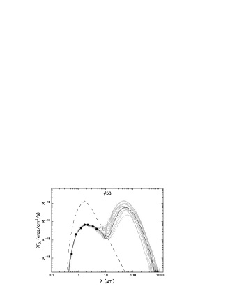
Figure 11.— SED fitting using the model of Robitaille et al. (2007) for (left) LDN1657A-3, from Linz et al. (2010), and (right) a typical Class II-type source. The ID no. corresponds to the IDs in the YSO table (Table 2). The black dots are our the data points. The solid black line shows the best fitted model, while the grey lines show the consecutive good fits for $\chi^{2}-\chi^{2}_{min}~{}(per~{}data~{}point)<3$. The dashed line shows the fit for the photosphere of the central source for the best fit model. The photosphere fit is assuming that there is no circumstellar dust, however, interstellar reddening has been accounted for.

Two of the PMS sources detected by Linz et al. (2010) - LDN1657A-2, & LDN1657A-3 - had WISE counterparts. LDN1657A-3 was also detected at NIR wavelengths. Using the flux values given for these sources at longer wavelengths from Linz et al. (2010), we could further constrain the physical parameters of these sources. The source with ID “1” in our SED table (Table 3) gives the values for LDN1657A-2, while “2” gives those for LDN1657A-3. Figure 11 shows examples of SEDs with the resulting models for LDN1657A-3 and a typical Class-II like source.

It must be kept in mind that the SED results are only representative of the actual values and should not be taken too literally. Out of a database of 200000 YSO models (each for a different set of parameter values), the model simply finds the closest matches for a particular source entered by the user. Any grid of models will have inherent limitations, which could give rise to pseudo-trends in the results. The models are for isolated objects and thus could be misleading when we have unresolved multiple point sources. Moreover, the model assumes same physics for stellar masses from 0.1 to 50 M_⊙. Robitaille (2008) provides a succinct summary of the caveats inherent in this modelling. Nevertheless, we can still use the results to glean general information about the mass and age ranges of our sources. As can be seen from Table 3, most of the sources have stellar ages in the range 0.05 to 1 Myr and masses in 0.2 to 2.5 M_⊙ range. The outliers are expectedly the more evolved H$\alpha$ emission line stars, whose ages vary upto 5 Myr, and stellar masses are $\sim$ 2.5$-$5 M_⊙. We see a few very low mass (3 sources with masses $<$ 0.5 M_⊙) and extremely young sources (9 sources with ages $<10^{5}$ yr, out of which 6 are CTTS) as well. The disk accretion rate for most of the H$\alpha$ emission line sources is in the range of $\sim$ 10^-9-10^-11 M_⊙ yr^-1, which is less than that of CTTS $\sim$ 10^-7-10^-9 M_⊙ yr^-1, though it would be prudent to treat these values with caution owing to a lack of FIR and submillimetre data points. A few of our sources, ID no.s 39, 55, 61, 81, 83, 94, 95, and 97 (Table 2), were better fitted by stellar models of a heavily extincted central star, and are thus not included here. Hence, we find that our age and mass estimations are mostly consistent with those derived from the optical CM diagram and the mass spectrum above.

5.7. Spatial distribution of the YSOs

Figure 12 shows the spatial distribution of the YSOs from our IRSF and grism slitless spectroscopy data. Red circles denote the sources with $H-K>1$, sources with $1\geq H-K>0.6$ have been shown with magenta crosses, blue circles denote the Class II-like objects detected from our CC diagram, while the white crosses show the location of the H$\alpha$ emission line stars from grism slitless spectroscopy. The central ionizing source HD 53623 (catalog ) is shown with a green square. Forbrich et al. (2004) had found a young, intermediate mass protostar named UYSO1 at the north-west border of the H ii region, towards the cold dark cloud LDN1657A (catalog ). The location of UYSO1, which was further resolved into two protostars (Forbrich et al., 2009), has been denoted by a green plus sign. In addition, a recent Herschel PACS and SPIRE mapping of the region around UYSO1 identified five cool and compact FIR sources, of masses of the order of a few solar masses, hidden in the dark cloud (Linz et al., 2010). They have been marked by green circles. Most of the YSOs identified by us lie in the molecular cloud region traced by ¹²CO molecular emission (see Section 4.3 & Figure 6), along the concave arc facing the north-eastern corner.

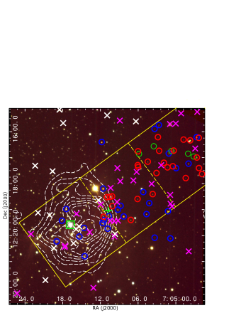
Figure 12.— Color composite showing the spatial distribution of the YSOs, made using IRSF J (blue), H (green), and $K_{\rm S}$ (red) band images. The H$\alpha$ emission line stars have been denoted by white crosses, Class II-like sources by blue circles, sources with $1\geq H-K>0.6$ with magenta crosses, and sources with $H-K>1$ by red circles. The green square marks the position of the central ionizing star HD 53623. UYSO1 (Forbrich et al., 2004) has been marked with a green plus sign, while the cool, compact sources from Linz et al. (2010) by green circles. 1280 MHz GMRT contours ($\sim$ 25${}^{{}^{\prime\prime}}$ resolution) showing the champagne flow have been shown in dashed white lines. The three sub-regions denoted by the yellow boxes show an increasing fraction of redder sources in the sub-regions as we move from the ionizing star towards the north-western direction. The dashed yellow lines are drawn at a distance of 80${}^{{}^{\prime\prime}}$ and 220${}^{{}^{\prime\prime}}$ from the ionizing star, respectively.

We have divided the region into three sub-regions which show increasing infrared excess from the south-east towards the north-west direction. This indicates an evolutionary sequence, thereby suggesting a possible decreasing age gradient towards that direction. The youngest stars, i.e. those with $H-K>0.6$ mostly lie towards the north-west direction, followed by a concentration of Class II-like objects and then the H$\alpha$ emission line stars towards the ionizing region. Even among the stars with $H-K>0.6$, the redder sources ($H-K>1$) were found to be lying towards the north-west, with a decreasing color sequence towards the ionizing source. Also, the 5 sources found by Herschel mapping are cooler than the massive object UYSO1 (Linz et al., 2010), thereby indicating that they are younger than UYSO1. We tried to quantify the infrared excess ($H-K$) for increasing distances of the sources from the ionizing star HD 53623. Figure 13 shows a plot of $H-K$ color versus distance. The graph is divided into three regions as shown by three boxes in Figure 12, with the average $H-K$ color calculated for each of them. The average color was found to increase as we move away from the ionizing star, thereby indicating that the sources in general, are younger at larger distances from the central region.

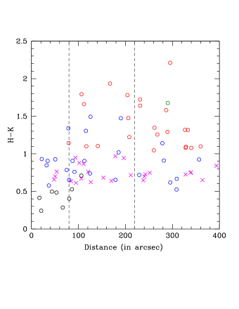
Figure 13.— The variation of $H-K$ color with distance from the star HD 53623. The H$\alpha$ emission line stars have been denoted by black circles, Class II-like sources by blue circles, sources with $1\geq H-K>0.6$ with magenta crosses, and sources with $H-K>1$ by red circles. Green circle denotes LDN1657A-3 source.

This distribution of YSOs, with relatively larger NIR excess at larger radial distances, could be indicative of probable triggered star formation, which seems to have propagated from the ionizing source towards the north-west.

6. Star formation scenario

Star formation in a molecular cloud is more active during the first few million years of cloud time. Subsequent to that, the gas in molecular cloud dissipates and further star formation no longer takes place. However, these types of molecular cloud complexes can still have star formation at the interface of the H ii region created by OB stars and the molecular gas. In Sh2-297 (catalog ) region, the spatial distribution of the YSOs and infrared excess calculations (Section 5.7) suggest an evolutionary sequence of sources from the ionizing region towards the cold, dark cloud LDN1657A (catalog ), with a majority of YSOs distributed at the western and north-western border of Sh2-297 (catalog ).

One of the conditions for the massive star HD 53623 (catalog ) to have influenced the formation of YSOs in the region is that the age of the H ii region and associated sources should be of the order of, or greater than, the age of the YSOs in the triggered region. However, it is difficult to estimate the age of YSOs as very few of them have optical counterparts. Nonetheless, we tried to estimate the age of the few sources which have optical counterparts in Section 5.4. Age estimation using IR data could be misleading because IR emission arises not only from the photosphere, but also the circumstellar disk of the YSOs. We tried to constrain the age of embedded YSOs with the SED fitting models, though due to the lack of sufficient data points, the estimated ages are uncertain. However, they can still be used as quantitative indicators of stellar youth. Our analysis shows the mean age of YSOs to be $\sim$ 1 Myr, which is of the order of the dynamical age of the H ii region of 1.07 $\pm$ 0.31 Myr, considering the uncertainties in age estimation. Our SED results (Table 3) also point out that barring 6 sources (all being H$\alpha$ emission line sources; possibly associated with the evolved H ii region), the other 22 sources have ages less than 1.07 Myr (majority of them are located in the dark cloud at the western border of Sh2-297 (catalog )). The protostellar source detected by Forbrich et al. (2009), and the cool, compact sources detected by Linz et al. (2010) also show recent star formation occurring in the dark cloud. The dynamical age of the outflow for UYSO1, which was constrained by Forbrich et al. (2009) as $<$ 10⁴ yr, and its location at the immediate interface of Sh2-297 (catalog ) supports our notion of triggered star formation by the expanding H ii region.

To examine if the collect-and-collapse due to the ionizing star is possibly at work in the region, we compare the observed properties with the analytical model by Whitworth et al. (1994, Section 5) for star formation at the periphery of an expanding H ii region. The model gives the expressions for the time when the fragmentation starts (t_frag), and the radius at the time of fragmentation (r_frag). The value of $a_{s}$ (isothermal sound speed in the shocked layer), which varies from 0.2 to 0.6 km s^-1, was taken to be 0.2 km s^-1 for our calculations. Using the values of $S_{*}$ and $n_{o}$ calculated in previous section (Section 4.2), we obtained $t_{frag}$ $\approx$ 1.27 Myr and $r_{frag}$ $\approx$ 1.70 pc. This would suggest that fragmentation would start at a radius of 1.70 pc, whereas the stellar sources found are within a 1.70 pc radius of the massive star HD 53623 (catalog ). However, the distance of the YSOs is the projected distance and the actual distance could be larger. Taking the present mean age of the YSOs as $\sim$ 1 Myr and the fragmentation time as calculated, it would imply that the age difference between the YSOs and HD 53623 (catalog ) ($\sim$ 5 $\pm$ 3 Myr) is $>$ 2 Myr. Though this $t_{frag}$ calculation suggests that this H ii region could be old enough to lead to star formation by collect-and-collapse process, the morphology of the region makes this process unlikely. Moreover, we have assumed the lowest value of isothermal sound speed for our calculations (0.2 km s^-1). A higher value of $a_{s}$ will only further increase the fragmentation time and radius and make a collect-and-collapse scenario unlikelier. Also, the YSOs are not exclusively associated with the PAH emission that we see around this region (Figure 6). PAH regions represent the compressed neutral matter between the ionization and shock fronts. The YSOs extend well beyond the PAH emission, as is evident from our MSX 8.28 $\mu$m contours (which, in addition, contains continuum emission too). This is distinctly separate from the star forming regions of, for example, Deharveng et al. (2005) where young sources and condensations have been observed along the PAH ring. It should be noted that, in an ideal case, one would expect regularly-spaced-clumps/protostars of very similar ages distributed along the periphery of the H ii region, mostly along the material swept-up by the expanding ionization front. This is definitely not the case here. It therefore appears that the collect-and-collapse process due to the star HD 53623 is most likely not involved in the star formation in this region.

Alternatively, it is possible that the star formation observed at the north-western border of Sh2-297 is probably due to some other processes. The formation of YSOs in the dark cloud area could partly be due to the influence of expanding H ii region Sh2-297 by RDI (radiation driven implosion) mechanism (most likely upto the edge and its vicinity) (Bertoldi, 1989; Lefloch & Lazareff, 1994), and partly due to supernova induced star formation as discussed by Herbst & Assousa (1977) (the distant YSOs possibly having formed by this process). The YSOs are distributed along the concave arc (see Section 5.7) of the molecular cloud traced by ¹²CO, and seem to have an age sequence. It appears that the supernova might have swept the molecular material and led to its piling up along the arc. Therefore, as the material might have collected along the arc, beginning from the edge of Sh2-297 towards the north-west, star formation could have occured at different epochs. The plausible location of the supernova ($\alpha_{1950}$ $\sim$ 07^h08^m, $\delta_{1950}$ $\sim$ -11.2^o, Reynolds & Ogden, 1978) and the derived age of the supernova remnant - 0.5 Myr (Herbst & Assousa, 1977) - lend weight to this hypothesis.

To better understand the star formation and the effect of the massive star on the Sh2-297 (catalog ) region, we need much deeper, wider and longer wavelength observations for better statistics (so as to constrain mass and luminosity functions of the embedded YSOs), and to carry out a study of YSOs along the arc of molecular material connecting Sh2-297 (catalog ) to the larger region. It would also be helpful to carry out a radial velocity study and spectroscopic observations for a wider area to constrain the membership, age and spectral type of the YSOs. This would confirm their relative evolutionary status’, identify possible clusters, and help put the relevant triggered star formation process on a firm footing.

7. Conclusions

In this paper, we have carried out a multiwavelength study of the star-forming region Sh2-297 (catalog ). Our main conclusions are as follows :

1. We identified the spectral class of the central ionizing star HD 53623 (catalog ), using optical spectroscopic data. The prominence of He I lines in our spectra indicate a spectral type of B0V. Our optical spectroscopic results are consistent with the radio continuum data results.

2. Using the radio data for 610, 1280, & 1420 MHz, the physical parameters of the region were derived. Taking the extent of the H ii region to be 1.6 pc (5${}^{{}^{\prime}}$), the emission measure was calculated to be 9.15 $\pm$ 0.56 $\times$ 10⁵ cm^-6 pc, and thereby the electron density as 756 $\pm$ 46 cm^-3. These low values of emission measure and the electron density confirm that this is indeed a classical H ii region. The strömgren radius was calculated to be 0.051 $\pm$ 0.002 pc and the dynamical timescale to be 1.07 $\pm$ 0.31 Myr.

3. The grism slitless spectroscopic image was used to identify the H$\alpha$ emission line stars; NIR CC diagram (J-H/H-K) to identify the Class II-type objects, and the NIR CM diagram (K/H-K) to identify the red sources ($H-K>0.6$) in our field. The average extinction in the field was calculated to be 2.70 mag.

4. We estimated the age and mass of the YSOs using our optical CM diagram (V/V-I), besides using the NIR mass spectrum to estimate the mass range. Age was found to be in the range 0.5 to 2 Myr, with the average age being $\sim$ 1 Myr. The mass was estimated to be $\sim$ 0.1 to 2 M_⊙, with a few outliers $\sim$ 3 M_⊙.

5. We studied the evolutionary status of some of the sources from Linz et al. (2010), red sources, Class II-type objects, and H$\alpha$ emission line stars using the SED model of Robitaille et al. (2007). The models predict - for most of the sources - stellar age in the range 0.05$-$1 Myr, stellar mass in the range 0.2$-$2.5 M_⊙, and disk accretion rate $\sim$ 10${}^{-7}-$10^-11 M_⊙yr^-1. A few H$\alpha$ emission line stars, which are most evolved YSOs in the field, have stellar ages upto 5 Myr, and masses $\sim$ 2.5$-$5 M_⊙.

6. The spatial distribution of the YSOs indicates a possible evolutionary sequence, in the sense that youngest sources are distributed away from the ionizing source. This could be evidence in support of triggered star formation in the region. The star formation seems to have propagated from the ionizing source towards the cloud LDN1657A (catalog ), which is further supported by the presence of massive protostar UYSO1 discovered by Forbrich et al. (2004), and cool, compact sources discovered by Linz et al. (2010), which are located away from the ionizing source.

We thank the anonymous referee for a very thorough and critical reading of our manuscript. The useful comments and suggestions made by the referee greatly improved the scientific content of the paper. The authors thank the staff of HCT, operated by Indian Institute of Astrophysics (Bangalore); IGO at Girawali, operated by Inter University Centre for Astronomy & Astrophysics (IUCAA), Pune; IRSF at South Africa in joint partnership between S.A.A.O and Nagoya University of Japan; and GMRT managed by National Center for Radio Astrophysics of the Tata Institute of Fundamental Research (TIFR) for their assistance and support during observations. This paper used data from the NRAO VLA Archive Survey (NVAS). The NVAS can be accessed through http://www.aoc.nrao.edu/$\sim$vlbacald/. MT is supported by KAKENHI 22000005. KKM acknowledges support from a Marie Curie IRSES grant (230843) under the auspices of which some part of this work was carried out.

Table 2Optical & infrared magnitudes for the YSOs

ID	RA	Dec.	V	I	J	H	KS	w1	w2	w3
	(J2000)	(J2000)
LDN1657A-2 & 3 from Linz et al. (2010)
1	07:04:58.030	-12:16:50.80	$\cdots$	$\cdots$	$\cdots$	$\cdots$	$\cdots$	14.12 $\pm$ 0.08	10.78 $\pm$ 0.02	8.62 $\pm$ 0.09
2	07:05:00.665	-12:16:45.13	$\cdots$	$\cdots$	16.85 $\pm$ 0.10	14.67 $\pm$ 0.05	12.96 $\pm$ 0.04	11.12 $\pm$ 0.01	9.73 $\pm$ 0.01	7.17 $\pm$ 0.02
YSOs with $H-K>0.6$
3	07:04:55.818	-12:17:37.90	$\cdots$	$\cdots$	$\cdots$	16.62 $\pm$ 0.03	15.51 $\pm$ 0.09	$\cdots$	$\cdots$	$\cdots$
4	07:04:56.305	-12:17:24.14	$\cdots$	$\cdots$	$\cdots$	16.82 $\pm$ 0.03	15.47 $\pm$ 0.07	14.78 $\pm$ 0.11	13.69 $\pm$ 0.10	$\cdots$
5	07:04:56.334	-12:16:14.28	$\cdots$	$\cdots$	$\cdots$	17.32 $\pm$ 0.04	16.18 $\pm$ 0.13	$\cdots$	$\cdots$	$\cdots$
6	07:04:56.580	-12:15:14.47	$\cdots$	$\cdots$	$\cdots$	16.67 $\pm$ 0.02	15.80 $\pm$ 0.10	14.63 $\pm$ 0.08	$\cdots$	$\cdots$
7	07:04:56.634	-12:16:59.69	$\cdots$	$\cdots$	17.39 $\pm$ 0.04	14.95 $\pm$ 0.01	13.60 $\pm$ 0.02	12.64 $\pm$ 0.03	$\cdots$	$\cdots$
8	07:04:56.898	-12:16:39.00	$\cdots$	$\cdots$	$\cdots$	15.87 $\pm$ 0.07	15.09 $\pm$ 0.06	13.71 $\pm$ 0.06	12.49 $\pm$ 0.08	$\cdots$
9	07:04:57.702	-12:16:20.06	$\cdots$	$\cdots$	$\cdots$	13.32 $\pm$ 0.01	12.21 $\pm$ 0.01	11.06 $\pm$ 0.02	10.91 $\pm$ 0.02	$\cdots$
10	07:04:57.927	-12:20:36.37	$\cdots$	$\cdots$	$\cdots$	17.14 $\pm$ 0.05	16.12 $\pm$ 0.13	$\cdots$	$\cdots$	$\cdots$
11	07:04:58.407	-12:17:47.23	$\cdots$	$\cdots$	$\cdots$	16.60 $\pm$ 0.03	15.27 $\pm$ 0.06	14.78 $\pm$ 0.10	14.21 $\pm$ 0.16	$\cdots$
12	07:04:58.749	-12:16:18.35	$\cdots$	$\cdots$	$\cdots$	16.27 $\pm$ 0.03	15.15 $\pm$ 0.06	$\cdots$	$\cdots$	$\cdots$
13	07:04:59.150	-12:15:17.78	$\cdots$	$\cdots$	$\cdots$	16.73 $\pm$ 0.03	16.05 $\pm$ 0.14	$\cdots$	$\cdots$	$\cdots$
14	07:04:59.994	-12:15:41.34	$\cdots$	$\cdots$	17.65 $\pm$ 0.03	16.12 $\pm$ 0.02	15.34 $\pm$ 0.06	$\cdots$	$\cdots$	$\cdots$
15	07:05:00.319	-12:16:43.75	$\cdots$	$\cdots$	$\cdots$	15.69 $\pm$ 0.03	13.44 $\pm$ 0.02	$\cdots$	$\cdots$	$\cdots$
16	07:05:00.599	-12:18:52.50	$\cdots$	$\cdots$	17.56 $\pm$ 0.03	16.25 $\pm$ 0.02	15.52 $\pm$ 0.08	$\cdots$	$\cdots$	$\cdots$
17	07:05:00.826	-12:18:46.47	$\cdots$	$\cdots$	$\cdots$	16.80 $\pm$ 0.05	16.12 $\pm$ 0.13	$\cdots$	$\cdots$	$\cdots$
18	07:05:00.881	-12:18:26.03	$\cdots$	$\cdots$	17.55 $\pm$ 0.05	16.86 $\pm$ 0.04	16.10 $\pm$ 0.14	14.59 $\pm$ 0.10	$\cdots$	$\cdots$
19	07:05:00.919	-12:15:42.37	19.65 $\pm$ 0.01	15.29 $\pm$ 0.01	12.47 $\pm$ 0.01	10.83 $\pm$ 0.01	10.07 $\pm$ 0.01	9.61 $\pm$ 0.01	9.47 $\pm$ 0.01	$\cdots$
20	07:05:01.313	-12:17:22.48	$\cdots$	$\cdots$	$\cdots$	16.83 $\pm$ 0.03	15.45 $\pm$ 0.08	14.72 $\pm$ 0.10	$\cdots$	$\cdots$
21	07:05:01.873	-12:17:11.83	$\cdots$	$\cdots$	$\cdots$	16.95 $\pm$ 0.04	15.87 $\pm$ 0.12	14.82 $\pm$ 0.16	$\cdots$	$\cdots$
22	07:05:02.311	-12:17:17.60	$\cdots$	$\cdots$	$\cdots$	16.99 $\pm$ 0.03	16.21 $\pm$ 0.13	$\cdots$	$\cdots$	$\cdots$
23	07:05:02.637	-12:16:44.26	$\cdots$	$\cdots$	$\cdots$	16.29 $\pm$ 0.02	14.99 $\pm$ 0.05	$\cdots$	14.33 $\pm$ 0.24	$\cdots$
24	07:05:02.833	-12:16:12.72	$\cdots$	$\cdots$	$\cdots$	17.34 $\pm$ 0.04	15.72 $\pm$ 0.09	14.46 $\pm$ 0.18	13.69 $\pm$ 0.10	$\cdots$
25	07:05:03.666	-12:18:24.20	$\cdots$	$\cdots$	$\cdots$	16.09 $\pm$ 0.02	14.27 $\pm$ 0.03	13.23 $\pm$ 0.05	12.15 $\pm$ 0.05	$\cdots$
26	07:05:03.832	-12:18:00.40	$\cdots$	$\cdots$	16.64 $\pm$ 0.02	15.10 $\pm$ 0.01	14.35 $\pm$ 0.03	13.12 $\pm$ 0.06	$\cdots$	$\cdots$
27	07:05:04.448	-12:17:09.32	$\cdots$	$\cdots$	$\cdots$	15.98 $\pm$ 0.01	14.31 $\pm$ 0.03	13.26 $\pm$ 0.05	12.57 $\pm$ 0.05	$\cdots$
28	07:05:05.984	-12:17:21.69	$\cdots$	$\cdots$	$\cdots$	16.88 $\pm$ 0.03	15.37 $\pm$ 0.06	$\cdots$	$\cdots$	$\cdots$
29	07:05:05.995	-12:16:45.27	$\cdots$	$\cdots$	$\cdots$	17.15 $\pm$ 0.04	15.39 $\pm$ 0.07	14.65 $\pm$ 0.14	$\cdots$	$\cdots$
30	07:05:06.044	-12:17:17.39	$\cdots$	$\cdots$	$\cdots$	16.91 $\pm$ 0.04	15.65 $\pm$ 0.09	$\cdots$	$\cdots$	$\cdots$
31	07:05:06.075	-12:18:35.45	$\cdots$	$\cdots$	$\cdots$	16.55 $\pm$ 0.03	14.59 $\pm$ 0.03	13.27 $\pm$ 0.09	12.06 $\pm$ 0.07	$\cdots$
32	07:05:06.216	-12:17:33.02	$\cdots$	$\cdots$	18.25 $\pm$ 0.07	16.46 $\pm$ 0.03	15.48 $\pm$ 0.08	$\cdots$	$\cdots$	$\cdots$
33	07:05:06.735	-12:17:52.68	$\cdots$	$\cdots$	$\cdots$	16.85 $\pm$ 0.03	15.85 $\pm$ 0.11	$\cdots$	$\cdots$	$\cdots$
34	07:05:07.139	-12:19:23.87	$\cdots$	$\cdots$	17.59 $\pm$ 0.05	15.48 $\pm$ 0.01	14.34 $\pm$ 0.03	$\cdots$	$\cdots$	$\cdots$
35	07:05:08.827	-12:17:54.66	$\cdots$	$\cdots$	17.69 $\pm$ 0.03	16.31 $\pm$ 0.02	15.60 $\pm$ 0.08	$\cdots$	$\cdots$	$\cdots$
36	07:05:08.890	-12:15:34.44	$\cdots$	$\cdots$	$\cdots$	16.89 $\pm$ 0.06	16.00 $\pm$ 0.13	15.72 $\pm$ 0.27	$\cdots$	$\cdots$
37	07:05:09.181	-12:19:25.46	$\cdots$	$\cdots$	16.00 $\pm$ 0.01	14.15 $\pm$ 0.01	13.26 $\pm$ 0.01	$\cdots$	$\cdots$	$\cdots$
38	07:05:09.283	-12:17:24.01	$\cdots$	$\cdots$	17.70 $\pm$ 0.04	16.31 $\pm$ 0.02	15.63 $\pm$ 0.09	$\cdots$	$\cdots$	$\cdots$
39	07:05:09.326	-12:18:42.24	$\cdots$	$\cdots$	14.38 $\pm$ 0.04	12.84 $\pm$ 0.06	12.05 $\pm$ 0.05	10.88 $\pm$ 0.06	10.12 $\pm$ 0.06	$\cdots$
40	07:05:09.749	-12:20:02.05	$\cdots$	$\cdots$	17.45 $\pm$ 0.04	16.22 $\pm$ 0.02	15.52 $\pm$ 0.08	$\cdots$	$\cdots$	$\cdots$
41	07:05:09.811	-12:19:26.43	$\cdots$	$\cdots$	$\cdots$	16.97 $\pm$ 0.04	16.06 $\pm$ 0.14	$\cdots$	$\cdots$	$\cdots$
42	07:05:10.071	-12:18:51.91	$\cdots$	$\cdots$	$\cdots$	18.02 $\pm$ 0.10	16.19 $\pm$ 0.14	$\cdots$	$\cdots$	$\cdots$
43	07:05:10.124	-12:18:29.40	$\cdots$	$\cdots$	16.65 $\pm$ 0.01	14.53 $\pm$ 0.01	13.40 $\pm$ 0.02	$\cdots$	$\cdots$	$\cdots$
44	07:05:10.358	-12:18:09.88	$\cdots$	$\cdots$	17.46 $\pm$ 0.03	16.26 $\pm$ 0.02	15.61 $\pm$ 0.09	$\cdots$	$\cdots$	$\cdots$
45	07:05:10.395	-12:19:25.70	$\cdots$	$\cdots$	$\cdots$	16.64 $\pm$ 0.06	15.66 $\pm$ 0.10	11.20 $\pm$ 0.10	10.85 $\pm$ 0.12	5.12 $\pm$ 0.07
46	07:05:10.481	-12:18:30.70	$\cdots$	$\cdots$	$\cdots$	17.59 $\pm$ 0.07	15.89 $\pm$ 0.10	$\cdots$	$\cdots$	$\cdots$
47	07:05:11.475	-12:19:16.58	$\cdots$	$\cdots$	$\cdots$	16.55 $\pm$ 0.06	15.38 $\pm$ 0.13	$\cdots$	$\cdots$	$\cdots$
48	07:05:11.946	-12:18:48.14	$\cdots$	$\cdots$	15.46 $\pm$ 0.01	13.99 $\pm$ 0.01	13.32 $\pm$ 0.01	$\cdots$	$\cdots$	$\cdots$
49	07:05:13.678	-12:19:51.96	$\cdots$	$\cdots$	15.89 $\pm$ 0.01	14.52 $\pm$ 0.01	13.83 $\pm$ 0.02	11.81 $\pm$ 0.13	11.10 $\pm$ 0.10	$\cdots$
50	07:05:17.596	-12:20:23.48	$\cdots$	$\cdots$	$\cdots$	16.88 $\pm$ 0.04	16.14 $\pm$ 0.13	$\cdots$	$\cdots$	$\cdots$
51	07:05:17.668	-12:20:26.39	$\cdots$	$\cdots$	17.47 $\pm$ 0.04	16.66 $\pm$ 0.03	15.86 $\pm$ 0.11	$\cdots$	$\cdots$	$\cdots$
52	07:05:23.035	-12:19:56.15	$\cdots$	$\cdots$	17.03 $\pm$ 0.02	16.28 $\pm$ 0.02	15.64 $\pm$ 0.08	$\cdots$	$\cdots$	$\cdots$
Class II-type sources
53	07:04:56.673	-12:16:12.77	20.19 $\pm$ 0.03	16.94 $\pm$ 0.01	15.81 $\pm$ 0.01	14.25 $\pm$ 0.01	13.29 $\pm$ 0.02	12.04 $\pm$ 0.02	11.43 $\pm$ 0.02	$\cdots$
54	07:04:57.964	-12:17:13.85	$\cdots$	$\cdots$	16.08 $\pm$ 0.01	15.07 $\pm$ 0.01	14.37 $\pm$ 0.04	14.14 $\pm$ 0.06	12.92 $\pm$ 0.06	$\cdots$
55	07:04:59.938	-12:17:24.19	$\cdots$	$\cdots$	17.61 $\pm$ 0.05	15.61 $\pm$ 0.03	14.43 $\pm$ 0.04	13.17 $\pm$ 0.04	12.94 $\pm$ 0.07	$\cdots$
56	07:05:00.844	-12:20:06.48	$\cdots$	$\cdots$	17.20 $\pm$ 0.04	16.32 $\pm$ 0.02	15.70 $\pm$ 0.09	$\cdots$	$\cdots$	$\cdots$
57	07:05:01.117	-12:16:50.42	$\cdots$	$\cdots$	17.35 $\pm$ 0.04	16.08 $\pm$ 0.03	15.13 $\pm$ 0.06	$\cdots$	$\cdots$	$\cdots$
58	07:05:01.230	-12:19:03.69	20.20 $\pm$ 0.03	16.73 $\pm$ 0.01	14.83 $\pm$ 0.01	13.60 $\pm$ 0.01	12.85 $\pm$ 0.01	11.77 $\pm$ 0.02	11.11 $\pm$ 0.02	$\cdots$
59	07:05:02.673	-12:15:44.75	$\cdots$	$\cdots$	16.70 $\pm$ 0.02	15.84 $\pm$ 0.01	15.28 $\pm$ 0.07	$\cdots$	$\cdots$	$\cdots$
60	07:05:03.364	-12:15:53.58	$\cdots$	$\cdots$	17.78 $\pm$ 0.04	16.75 $\pm$ 0.03	16.09 $\pm$ 0.14	$\cdots$	$\cdots$	$\cdots$
61	07:05:04.206	-12:18:45.13	$\cdots$	$\cdots$	17.90 $\pm$ 0.06	15.30 $\pm$ 0.01	13.80 $\pm$ 0.02	12.44 $\pm$ 0.04	11.37 $\pm$ 0.03	$\cdots$
62	07:05:04.644	-12:19:10.39	$\cdots$	$\cdots$	15.96 $\pm$ 0.02	14.82 $\pm$ 0.01	14.13 $\pm$ 0.02	13.46 $\pm$ 0.13	$\cdots$	$\cdots$
63	07:05:05.166	-12:18:19.49	$\cdots$	$\cdots$	17.43 $\pm$ 0.04	15.88 $\pm$ 0.02	14.82 $\pm$ 0.04	$\cdots$	$\cdots$	$\cdots$
64	07:05:08.269	-12:19:15.83	$\cdots$	$\cdots$	16.16 $\pm$ 0.01	13.69 $\pm$ 0.01	12.16 $\pm$ 0.01	10.41 $\pm$ 0.06	9.03 $\pm$ 0.03	$\cdots$
65	07:05:08.771	-12:18:51.26	$\cdots$	$\cdots$	16.67 $\pm$ 0.02	15.41 $\pm$ 0.02	14.64 $\pm$ 0.04	$\cdots$	$\cdots$	$\cdots$
66	07:05:09.197	-12:19:00.00	$\cdots$	$\cdots$	17.09 $\pm$ 0.03	15.29 $\pm$ 0.01	13.95 $\pm$ 0.02	11.16 $\pm$ 0.08	10.86 $\pm$ 0.17	$\cdots$
67	07:05:10.638	-12:19:15.02	$\cdots$	$\cdots$	17.04 $\pm$ 0.02	15.89 $\pm$ 0.03	15.10 $\pm$ 0.06	$\cdots$	$\cdots$	$\cdots$
68	07:05:10.818	-12:19:43.90	$\cdots$	$\cdots$	17.16 $\pm$ 0.04	15.83 $\pm$ 0.02	14.89 $\pm$ 0.05	$\cdots$	$\cdots$	$\cdots$
69	07:05:11.424	-12:19:24.36	$\cdots$	$\cdots$	16.93 $\pm$ 0.04	15.13 $\pm$ 0.01	13.76 $\pm$ 0.04	11.04 $\pm$ 0.10	10.45 $\pm$ 0.10	$\cdots$
70	07:05:11.541	-12:18:11.39	20.02 $\pm$ 0.05	16.58 $\pm$ 0.03	14.63 $\pm$ 0.01	13.09 $\pm$ 0.01	12.15 $\pm$ 0.01	$\cdots$	10.04 $\pm$ 0.08	$\cdots$
71	07:05:11.642	-12:19:30.95	$\cdots$	$\cdots$	15.10 $\pm$ 0.01	13.96 $\pm$ 0.01	13.14 $\pm$ 0.01	$\cdots$	$\cdots$	$\cdots$
72	07:05:11.774	-12:16:24.01	20.78 $\pm$ 0.05	17.95 $\pm$ 0.02	15.34 $\pm$ 0.01	13.72 $\pm$ 0.01	12.52 $\pm$ 0.01	11.27 $\pm$ 0.02	10.29 $\pm$ 0.02	7.89 $\pm$ 0.07
73	07:05:14.495	-12:20:47.57	$\cdots$	$\cdots$	15.25 $\pm$ 0.01	14.16 $\pm$ 0.01	13.47 $\pm$ 0.02	12.43 $\pm$ 0.12	11.65 $\pm$ 0.12	$\cdots$
74	07:05:14.610	-12:19:42.29	$\cdots$	$\cdots$	15.07 $\pm$ 0.01	13.62 $\pm$ 0.01	12.74 $\pm$ 0.01	$\cdots$	$\cdots$	$\cdots$
75	07:05:15.324	-12:20:02.05	$\cdots$	$\cdots$	17.17 $\pm$ 0.04	15.89 $\pm$ 0.01	14.95 $\pm$ 0.05	11.61 $\pm$ 0.22	11.30 $\pm$ 0.27	$\cdots$
76	07:05:17.419	-12:18:58.69	$\cdots$	$\cdots$	14.42 $\pm$ 0.01	13.49 $\pm$ 0.01	12.88 $\pm$ 0.01	11.95 $\pm$ 0.04	11.21 $\pm$ 0.06	$\cdots$
77	07:05:18.113	-12:19:25.47	$\cdots$	$\cdots$	17.25 $\pm$ 0.03	15.90 $\pm$ 0.01	14.94 $\pm$ 0.05	$\cdots$	$\cdots$	$\cdots$
78	07:05:18.950	-12:20:13.53	$\cdots$	$\cdots$	16.03 $\pm$ 0.05	14.93 $\pm$ 0.03	13.97 $\pm$ 0.03	$\cdots$	9.47 $\pm$ 0.05	$\cdots$
H$\alpha$ emission line sources
79	07:05:06.330	-12:15:36.38	17.43 $\pm$ 0.01	14.82 $\pm$ 0.01	12.95 $\pm$ 0.01	12.01 $\pm$ 0.01	11.33 $\pm$ 0.01	10.44 $\pm$ 0.01	9.84 $\pm$ 0.01	7.36 $\pm$ 0.03
80	07:05:09.652	-12:19:56.32	20.07 $\pm$ 0.03	16.18 $\pm$ 0.01	14.05 $\pm$ 0.01	12.77 $\pm$ 0.01	12.02 $\pm$ 0.01	10.91 $\pm$ 0.07	10.21 $\pm$ 0.07	$\cdots$
81	07:05:10.920	-12:15:22.46	$\cdots$	$\cdots$	15.11 $\pm$ 0.01	14.49 $\pm$ 0.01	14.11 $\pm$ 0.03	13.61 $\pm$ 0.04	13.12 $\pm$ 0.05	$\cdots$
82	07:05:12.292	-12:18:38.27	16.74 $\pm$ 0.01	14.37 $\pm$ 0.01	13.01 $\pm$ 0.01	12.06 $\pm$ 0.01	11.50 $\pm$ 0.01	11.05 $\pm$ 0.11	10.53 $\pm$ 0.12	$\cdots$
83	07:05:15.359	-12:19:39.02	$\cdots$	$\cdots$	13.13 $\pm$ 0.06	12.27 $\pm$ 0.06	11.99 $\pm$ 0.05	10.93 $\pm$ 0.12	10.27 $\pm$ 0.10	$\cdots$
84	07:05:15.840	-12:19:45.09	15.41 $\pm$ 0.14	14.39 $\pm$ 0.02	13.41 $\pm$ 0.01	12.55 $\pm$ 0.01	12.10 $\pm$ 0.01	$\cdots$	$\cdots$	$\cdots$
85	07:05:16.265	-12:20:17.61	$\cdots$	$\cdots$	14.32 $\pm$ 0.01	13.37 $\pm$ 0.01	12.84 $\pm$ 0.01	$\cdots$	$\cdots$	$\cdots$
86	07:05:17.904	-12:15:40.26	15.27 $\pm$ 0.01	14.17 $\pm$ 0.01	13.89 $\pm$ 0.01	13.65 $\pm$ 0.02	13.40 $\pm$ 0.03	12.86 $\pm$ 0.03	12.50 $\pm$ 0.04	$\cdots$
87	07:05:18.494	-12:15:09.22	17.35 $\pm$ 0.01	14.85 $\pm$ 0.01	14.00 $\pm$ 0.01	12.85 $\pm$ 0.01	11.95 $\pm$ 0.01	10.77 $\pm$ 0.01	9.97 $\pm$ 0.01	8.21 $\pm$ 0.03
88	07:05:19.389	-12:20:28.71	14.37 $\pm$ 0.01	12.92 $\pm$ 0.01	11.83 $\pm$ 0.01	11.11 $\pm$ 0.01	10.79 $\pm$ 0.01	10.09 $\pm$ 0.06	9.50 $\pm$ 0.05	$\cdots$
89	07:05:19.592	-12:17:31.48	16.82 $\pm$ 0.01	14.59 $\pm$ 0.01	13.38 $\pm$ 0.01	12.51 $\pm$ 0.01	12.10 $\pm$ 0.01	11.40 $\pm$ 0.01	10.74 $\pm$ 0.02	7.82 $\pm$ 0.03
90	07:05:20.068	-12:19:12.59	13.86 $\pm$ 0.01	12.69 $\pm$ 0.01	11.67 $\pm$ 0.01	10.92 $\pm$ 0.01	10.40 $\pm$ 0.01	9.82 $\pm$ 0.01	9.36 $\pm$ 0.01	6.62 $\pm$ 0.04
91	07:05:20.728	-12:21:42.69	17.11 $\pm$ 0.01	15.14 $\pm$ 0.01	13.83 $\pm$ 0.01	12.84 $\pm$ 0.01	12.15 $\pm$ 0.01	11.03 $\pm$ 0.02	10.38 $\pm$ 0.02	$\cdots$
92	07:05:21.912	-12:19:07.19	19.80 $\pm$ 0.02	15.92 $\pm$ 0.01	14.30 $\pm$ 0.01	13.44 $\pm$ 0.01	13.01 $\pm$ 0.01	12.53 $\pm$ 0.03	12.02 $\pm$ 0.03	$\cdots$
93	07:05:22.359	-12:17:18.63	18.23 $\pm$ 0.01	15.39 $\pm$ 0.01	14.17 $\pm$ 0.01	13.30 $\pm$ 0.01	12.84 $\pm$ 0.01	12.25 $\pm$ 0.02	11.62 $\pm$ 0.03	$\cdots$
H$\alpha$ emission line sources outside NIR FoV
94	07:05:12.139	-12:14:41.57	$\cdots$	$\cdots$	14.15 $\pm$ 0.04	13.26 $\pm$ 0.04	12.77 $\pm$ 0.03	12.26 $\pm$ 0.02	11.76 $\pm$ 0.02	9.38 $\pm$ 0.03
95	07:05:16.154	-12:14:55.90	18.57 $\pm$ 0.01	15.73 $\pm$ 0.01	14.24 $\pm$ 0.03	13.30 $\pm$ 0.03	12.77 $\pm$ 0.03	12.15 $\pm$ 0.02	11.53 $\pm$ 0.02	10.00 $\pm$ 0.09
96	07:05:23.669	-12:22:36.08	16.18 $\pm$ 0.01	14.14 $\pm$ 0.01	13.25 $\pm$ 0.03	12.48 $\pm$ 0.02	12.16 $\pm$ 0.02	11.89 $\pm$ 0.02	11.46 $\pm$ 0.03	8.33 $\pm$ 0.10
97	07:05:37.457	-12:21:17.32	$\cdots$	$\cdots$	13.98 $\pm$ 0.02	13.14 $\pm$ 0.02	12.73 $\pm$ 0.03	12.04 $\pm$ 0.05	11.34 $\pm$ 0.07	$\cdots$

References

- Alloin & Tenorio Tagle (1979) Alloin, D., & Tenorio Tagle, G. 1979, ESO Messenger, 18, 12
- Bertoldi (1989) Bertoldi, F. 1989, ApJ, 346, 735
- Bessell & Brett (1988) Bessell, M. S., & Brett, J. M. 1988, PASP, 100, 1134
- Beuther et al. (2008) Beuther, H., Semenov, D., Henning, T., & Linz, H. 2008, ApJ, 675, L33
- Bica et al. (2003) Bica, E., Dutra, C. M., Soares, J., & Barbuy, B. 2003, A&A, 404, 223
- Blitz (1980) Blitz, L. 1980, in Giant Molecular Clouds in the Galaxy, eds. M. G. Edmunds & P. M. Solomon, p.211
- Bonatto & Bica (2009) Bonatto, C., & Bica, E. 2009, MNRAS, 397, 1915
- Clariá (1974) Clariá, J. J. 1974, AJ, 79, 1022
- Cohen et al. (1981) Cohen, J. G., Frogel, J. A., Persson, S. E., & Elias, J. H. 1981, ApJ, 249, 481
- Deharveng et al. (2005) Deharveng, L., Zavagno, A., & Caplan, J. 2005, A&A, 433, 565
- Di Francesco et al. (2008) Di Francesco, J., Johnstone, D., Kirk, H., MacKenzie, T., & Ledwosinska, E. 2008, ApJS, 175, 277
- Felli & Churchwell (1972) Felli, M., & Churchwell, E. 1972, A&AS, 5, 369
- Felli & Harten (1981) Felli, M., & Harten, R. H. 1981, A&A, 100, 42
- Fich (1993) Fich, M. 1993, ApJS, 86, 475
- Forbrich et al. (2004) Forbrich, J., Schreyer, K., Posselt, B., Klein, R., & Henning, T. 2004, ApJ, 602, 843
- Forbrich et al. (2009) Forbrich, J., Stanke, T., Klein, R., et al. 2009, A&A, 493, 547
- Girardi et al. (2002) Girardi, L., Bertelli, G., Bressan, A., et al. 2002, A&A, 391, 195
- Gregorio-Hetem (2008) Gregorio-Hetem, J. 2008, Handbook of Star Forming Regions, Volume II: The Southern Sky ASP Monograph Publications, Vol. 5, ed. Bo Reipurth, p.1
- Haslam et al. (1982) Haslam, C. G. T., Salter, C. J., Stoffel, H., & Wilson, W. E. 1982, A&AS, 47, 1
- Herbst & Assousa (1977) Herbst, W., & Assousa, G. E. 1977, ApJ, 217, 473
- Herbst et al. (1978) Herbst, W., Racine, R., & Warner, J. W. 1978, ApJ, 223, 471
- Hillenbrand et al. (2008) Hillenbrand, L. A., Bauermeister, A., & White, R. J. 2008, in ASP Conf. Series Vol. 384, 200, 14th Cambridge Workshop on Cool Stars, Stellar Systems, and the Sun ed. G. T. van Belle
- Houk & Smith-Moore (1988) Houk, N., & Smith-Moore, M. 1988, Michigan Catalogue of Two-dimensional Spectral Types for the HD Stars, Volume 4 (Ann Arbor: Univ. Michigan)
- Jose et al. (2008) Jose, J., Pandey, A. K., Ojha, D.K., et al. 2008, MNRAS, 384, 1675
- Kainulainen et al. (2007) Kainulainen, J., Lehtinen, K., Väisänen, P., Bronfman, L., & Knude, J. 2007, A&A, 463, 1029
- Keenan et al. (2010) Keenan, R. C., Barger, A. J., Cowie, L. L., et al. 2010, ApJ, 723, 40
- Kim et al. (2004) Kim, B. G., Kawamura, A., Yonekura, Y., & Fukui, Y. 2004 , PASJ, 56, 313
- Koenig et al. (2012) Koenig, X. P., Leisawitz, D. T., Benford, D. J., et al. 2012, ApJ, 744, 130
- Lada & Adams (1992) Lada, C. J., & Adams, F. C. 1992, ApJ, 393, 278
- Lada et al. (1994) Lada, C. J., Lada, E. A., Clemens, D. P., & Bally, J. 1994, ApJ, 429, 694
- Landolt (1992) Landolt, A. U. 1992, AJ, 104, 340
- Lefloch & Lazareff (1994) Lefloch, B., & Lazareff, B. 1994, A&A, 289, 559
- Linz et al. (2010) Linz, H., Krause, O., Beuther, H., et al. 2010, A&A, 518, L123
- Massey et al. (1988) Massey, P., Strobel, K., Barnes, J. V., & Anderson, E. 1988, ApJ, 328, 315
- Meyer et al. (1997) Meyer, M. R., Calvet, N., & Hillenbrand, L. A. 1997, AJ, 114, 288
- Mezger & Henderson (1967) Mezger, P. G., & Henderson, A. P. 1967, ApJ, 147, 471
- Mezger et al. (1967) Mezger, P. G., Schraml, J., & Terzian, Y. 1967, ApJ, 150, 807
- Moran (1983) Moran, J. M. 1983, Rev. Mexicana Astron. Astrof., 7, 95
- Nagashima (1999) Nagashima, C., et al. 1999, in Proc. Star Formation 1999, ed. T. Nakamoto (Nagano: Nobeyama Radio Obs.), 387
- Nagayama (2003) Nagayama, T., et al. 2003, Proc. SPIE, 4841, 459
- Nakano et al. (1984) Nakano, M., Yoshida, S., & Kogure, T. 1984, PASJ, 36, 517
- Ojha et al. (2004a) Ojha, D. K., Ghosh, S. K., Kulkarni, V. K., et al. 2004a, A&A, 415, 1039
- Ojha et al. (2004b) Ojha, D. K., Tamura, M., Nakajima, Y., et al. 2004b, ApJ, 608, 797
- Ojha et al. (2004c) Ojha, D. K., Tamura, M., Nakajima, Y., et al. 2004c, ApJ, 616, 1042
- Ojha et al. (2011) Ojha, D. K., Samal, M. R., Pandey, A. K., et al. 2011, ApJ, 738, 156
- Panagia (1973) Panagia, N. 1973, AJ, 78, 929
- Pyatunina (1980) Pyatunina, T. B. 1980, Ap&SS, 67, 173
- Pyatunina & Taraskin (1986) Pyatunina, T. B., & Taraskin, Yu. M. 1986, Astron. Zhurnal, 63, 1098
- Reynolds & Ogden (1978) Reynolds, R. J., & Ogden, P. M. 1978, ApJ, 224, 94
- Robitaille et al. (2006) Robitaille, T. P., Whitney, B. A., Indebetouw, R., Wood, K., & Denzmore, P. 2006, ApJS, 167, 256
- Robitaille et al. (2007) Robitaille, T. P., Whitney, B. A., Indebetouw, R., & Wood, K. 2007, ApJS, 169, 328
- Robitaille (2008) Robitaille, T. P. 2008, ASPC, 387, 290
- Ruprecht (1966) Ruprecht, J. 1966, IAU Trans., 12B, 348
- Samal et al. (2007) Samal, M. R., Pandey, A. K., Ojha, D. K., et al. 2007, ApJ, 671, 555
- Samal et al. (2010) Samal, M. R., Pandey, A. K., Ojha, D. K., et al. 2010, ApJ, 714, 1015
- Sharma et al. (2007) Sharma, S., Pandey, A. K., Ojha, D. K., et al. 2007, MNRAS, 380, 1141
- Sharpless (1959) Sharpless, S. 1959, ApJS, 4, 257
- Siess et al. (2000) Siess, L., Dufour, E., & Forestini, M. 2000, A&A, 358, 593
- Spitzer (1978) Spitzer, L. 1978, Physical Processes in the Interstellar Medium (Wiley & Sons)
- Stahler & Palla (2004) Stahler, S. W., & Palla, F. 2004, The Formation of Stars (New York, Wiley-VCH)
- Stetson (1987) Stetson, P. B. 1987, PASP, 99, 191
- Strömgren (1939) Strömgren, B. 1939, ApJ, 89, 526
- Swarup et al. (1991) Swarup, G., Ananthakrishnan, S., Kapahi, V. K., et al. 1991, Current Science, 60, 95
- Tenorio Tagle et al. (1979) Tenorio Tagle, G., Yorke, H. W., & Bodenheimer, P. 1979, A&A, 80, 110
- Tjin A Djie et al. (2001) Tjin A Djie, H. R. E., van den Ancker, M. E., Blondel, P. F. C., et al. 2001, MNRAS, 325, 1441
- Van Den Bergh (1966) Van Den Bergh, S. 1966, AJ, 71, 990
- Vasyunina et al. (2011) Vasyunina, T., Linz, H., Henning, T., et al. 2011, A&A, 527, A88
- Vig et al. (2006) Vig, S., Ghosh, S. K., Kulkarni, V. K., Ojha, D. K., & Verma, R. P. 2006, ApJ, 637, 400
- Vrba et al. (1987) Vrba, F. J., Baierlein, R., & Herbst, W. 1987, ApJ, 317, 207
- Walborn & Fitzpatrick (1990) Walborn, N. R., & Fitzpatrick, E. L. 1990, PASP, 102, 379
- Ward-Thompson & Whitworth (2011) Ward-Thompson, D., & Whitworth, A. P. 2011, An Introduction to Star Formation (Cambridge Univ. Press)
- Weaver & Williams (1974) Weaver, H., & Williams, D. R. W. 1974, A&AS, 17, 1
- Whitney et al. (2003a) Whitney, B. A., Wood, K., Bjorkman, J. E., & Cohen, M. 2003a, ApJ, 598, 1079
- Whitney et al. (2003b) Whitney, B. A., Wood, K., Bjorkman, J. E., & Wolff, M. J. 2003b, ApJ, 591, 1049
- Whitworth et al. (1994) Whitworth, A. P., Bhattal, A. S., Chapman, S. J., Disney, M. J., & Turner, J. A. 1994, MNRAS, 268, 291
- Wright et al. (2010) Wright, E. L., Eisenhardt, P. R. M., Mainzer, A. K., et al. 2010, AJ, 140, 1868
- Zinnecker & Yorke (2007) Zinnecker, H., & Yorke, H. W. 2007, ARA&A, 45, 481