Dynamical tunneling-assisted coupling of high-Q deformed microcavities using a free-space beam

Abstract

We investigate the efficient free-space excitation of high-Q resonance modes in deformed microcavities via dynamical tunneling-assisted coupling. A quantum scattering theory is employed to study the free-space transmission properties, and it is found that the transmission includes the contribution from (1) the off-resonance background and (2) the on-resonance modulation, corresponding to the absence and presence of high-Q modes, respectively. The theory predicts asymmetric Fano-like resonances around high-Q modes in background transmission spectra, which are in good agreement with our recent experimental results. Dynamical tunneling across Kolmogorov-Arnol’d-Moser tori is further studied, which plays an essential role in the Fano-like resonance. This efficient free-space coupling holds potential advantages in simplifying experimental condition and exciting high-Q modes in higher-index-material microcavities.

I INTRODUCTION

Over last two decades, optical whispering-gallery-mode (WGM) microresonators (or microcavities) MicrocavitybyVahala with high quality factors and small mode volumes have promised lab-on-a-chip applications ranging from fundamental physics to various photonic devices, such as nonlinear optics PRL1986Chang ; Nature2002Vahala ; PRL2004Ilchenko ; Comb , cavity quantum electrodynamics Nature2006Kimble ; Nano2006Wang ; XiaoPRARap , cavity optomechanics PRL2005Vahala ; Nature2011Painter ; Science2012Wang , low-threshold microlasers PRA1996Haroche ; Microlasing ; APL2003Yang ; microlaserXiao and highly sensitive optical biosensors APL2002Arnold ; OL2006Fan ; PNAS2008Keng ; NatPho2010Yang ; XiaoOE . In these applications, traditionally light is coupled into the WGM microcavities by evanescent couplers, such as prisms PrismPRA1989 , tapered fibers FBOL1997 ; PRL2000Vahala and angle-polished fibers FbOL1999 , which have been validated to be highly efficient. In all of these coupling configurations, the microcavities are typically separated from the couplers by a distance of subwavelength because the evanescent fields of WGMs extend over a very short range. The use of the evanescent couplers, however, is not suitable in some important applications. For example, a higher-index-material microcavity PRL2004Ilchenko can not be efficiently excited by the tapered fiber due to phase mismatching. In addition, the external couplers degrade high-Q factors (defined as $\omega\tau$ where $\omega$ denotes the photon frequency and $\tau$ is its intracavity lifetime) in the case of the over-coupling regime, and they are not convenient in low-temperature chambers.

It has been demonstrated that WGMs in a specially designed deformed cavity can be directly excited by a free-space optical beam NonresonantPumping ; DynamicalAn . This direct free-space coupling is of importance because it is robust and requires less rigorous experimental condition than the evanescent couplers mentioned above. This efficient free-space coupling originates from breaking of rotational symmetry in deformed microcavities, which produces a highly directional emission assisted by the dynamical tunneling, different from the isotropic nature of a circular WGM cavity Nature ; DynamicalAn ; NonresonantPumping . According to the time reversion, i.e., the reversibility of light path, free-space beams at certain positions are expected to couple into the high-Q modes via chaotic modes when they are on resonance. So far, this type of free-space coupling technique has been demonstrated experimentally to reach a resonant efficiency exceeding $50\%$ OE2007Wang . A straightforward method to characterize free-space coupling is to study its transmission property, e.g., transmission spectrum. In this paper, we investigate the dynamical tunneling properties between the chaotic modes and the regular modes in detail, and predict transmission spectra of the free-space coupling by employing a quantum scattering theory. It is found that the spectrum can behave asymmetrically as Fano-like lineshape Fano , in good agreement with our recent experimental observation onpublish .

This paper is organized as follows. In Sec. II, we present the mechanism of dynamical tunneling-assisted coupling, and introduce a quantum scattering theory to predict a general transmission in free space. It is found that the free-space transmission spectrum includes the contribution from both the off-resonance background and the on-resonance modulation. In Sec. III, we study the off-resonance background transmission in the absence of the high-Q regular mode, corresponding to the unperturbed scattering. The off-resonance background transmission spectrum shows periodic modulations, which is in good agreement with both the numerical simulation and experimental results. In Sec. IV, the on-resonance transmission spectra are studied in detail. It is revealed that they depend strongly on (i) the additional phase when light travels in chaos trajectories and (ii) the rate of dynamical tunneling. Section V rigourously explains the chaotic states and the coupling strength, with which we deduce the condition of highest excitation efficiency. Section VI further investigates the KAM barriers which is predominant in the dynamical tunneling process. Section VII is a short summary of the paper.

II Dynamical tunneling-assisted coupling

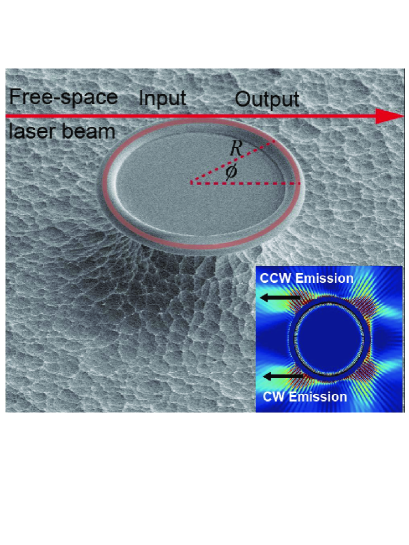
Figure 1: (Color online) Scanning electron microscope (SEM) view of a deformed silica microtoroid cavity. Here $R$ and $\phi$ are the polar coordinates in the cavity plane. Red arrow denotes the laser beam. Inset: False color illustration a resonant mode distribution obtained with wave simulation. The two black arrows denote the dominantly directional emission toward 180^∘ far-field direction. The strength outside the cavity is magnified for a clear show.

Without loss of generality, here we consider a two-dimensional deformed cavity made of silica with refractive index $\mathrm{n}=1.45$ as shown in Fig. 1, which has the boundary defined in polar coordinates as

$$R({\phi})=\begin{cases}R_{0}(1+\eta\displaystyle{\sum_{i=2,3}}a_{i}\cos^{i}\phi),&\text{for }\cos\phi\geq 0\\ R_{0}(1+\eta\displaystyle{\sum_{i=2,3}}b_{i}\cos^{i}\phi),&\text{for }\cos\phi<0\end{cases}$$ (1)

where $R_{0}$ and $\eta$ represent size and deformation parameters, respectively. Cavity shape parameters are set as $a_{2}=-0.1329$, $a_{3}=0.0948$, $b_{2}=-0.0642$, $b_{3}=-0.0224$. When $\eta=1$, a highly directional far-field universal pattern of high-Q modes has been predicted Zou and demonstrated experimentally Jiang . This emission characteristic is clearer by plotting the near-field pattern, as shown in the inset of Fig. 1. It can be seen that the two major emission positions are at $\phi=\pi/2$,and $3\pi/2$, corresponding to refractive escape from counter-clockwise (CCW) and clockwise (CW) modes, respectively. Thus, we expect with a time reversed way, an excitation beam focused on the primary emission position at $\phi=\pi/2$, as shown in Fig. 1, can eventually excite the CW resonant modes. To quantitatively study this chaos-assisted process, we use a quantum scattering theory to model the transmission, from which the coupling characteristic of the high-Q modes can be obtained.

Before studying the transmission spectrum, we first present the mechanism of dynamical tunneling-assisted coupling. Poincaré surface of section (PSOS) provides a simple and intuitive way to model the ray dynamics in deformed microcavities by recording the angular position $\phi$ and the incident angle $\chi$ of the rays, similar to billiards in quantum chaos. Except for an integrable ellipse-shaped cavity, the deformed microcavity has a mixed phase space including three types of structures: Kolmogorov-Arnol’d-Moser (KAM) tori, islands, and chaos sea, corresponding to quasi-periodicity, periodicity, and chaos motion of ray trajectories KAM , as shown in Fig. 2(a). KAM tori separate the PSOS into disjoint regions. As shown in Fig. 2(b), high-Q modes are usually localized in the regular regions bounded by a KAM torus OL1994 ; Science1998 ; QC . For such a localized high-Q mode, the excitation by a free-space beam is primarily attributed to two channels: (i) angular momentum tunneling and (ii) dynamical tunneling via chaos PRAAn . It has been demonstrated that the dynamical tunneling dominates, since the lifetime of photons that refract into the deformed cavity greatly increases along chaotic trajectories NonresonantPumping .

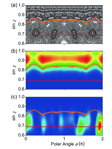
Figure 2: (Color online) (a) A typical PSOS of the deformed microcavity. The red solid line denotes the critical line defined as $\sin\chi=1/\mathrm{n}$. The orange dotted line stands for a KAM torus. (b) and (c) are normalized Husimi projection of the resonant mode and the excitation state, respectively.

In the system consisting of a microcavity and unbounded medium outside, the state $|\psi_{\omega}\rangle$ which describes the electromagnetic field excited by the incident beam satisfies stationary Schrödinger equation

$$H\left|\psi_{\omega}\right\rangle=\omega\left|\psi_{\omega}\right\rangle,$$ (2)

where $H$ stands for the system Hamiltonian. As mentioned above, not only chaotic modes but the regular mode can also be excited by an appropriate free-space beam thanks to the dynamical tunneling. This can be demonstrated by plotting the Husimi projection Husimi of the excitation state $\left|\psi_{\omega}\right\rangle$, as shown in Fig. 2(c). Thus $\left|\psi_{\omega}\right\rangle$ can be expanded as a linear combination of chaotic mode $\left|\mathrm{C}_{\omega}\right\rangle$ and regular mode $\left|\mathrm{WGM}\right\rangle$ WGM , with the form

$$|\psi_{\omega}\rangle=a_{\omega}|\mathrm{WGM}\rangle+\int\mathrm{d}\omega^{\prime}b_{\omega}(\omega^{\prime})|\mathrm{C}_{\omega^{\prime}}\rangle.$$ (3)

Throughout this paper, we use regular mode and chaotic mode to describe uncoupled states, and dynamical tunneling is the interaction between an uncoupled regular mode and uncoupled chaotic modes. The system Hamiltonian satisfies

$$\langle\mathrm{WGM}|H|\mathrm{WGM}\rangle =\omega_{0}-i\gamma/2,$$ (4a)

$$\langle\mathrm{C}_{\omega^{\prime}}|H|\mathrm{C}_{\omega}\rangle =\omega\delta(\omega^{\prime}-\omega),$$ (4b)

$$\langle\mathrm{C}_{\omega}|H|\mathrm{WGM}\rangle =V_{\omega}.$$ (4c)

Here $$\omega_{0} \omega \left|\mathrm{C}_{\omega}\right\rangle \left|\mathrm{WGM}\right\rangle V_{\omega} \gamma \gamma_{0} \gamma_{1} \left|\mathrm{C}_{\omega}\right\rangle \left|\mathrm{C}_{\omega}^{\perp}\right\rangle$$ and are the frequencies of the resonant regular mode and the incident light, respectively. The coupling coefficient between and , governed by the dynamical tunneling, is described by . The decay rate consists of the intrinsic loss and the chaos-assisted tunneling loss. In detail, the intrinsic decay rate is attributed to radiation, material absorption and scattering losses in the cavity, while the chaos-assisted decay rate describes tunneling into the chaotic modes other than . We denote them as .

In this paper, we consider the chaotic modes as continuum and use a standard quantum scattering model to interpret the transmission lineshape. Here we assume that $|\mathrm{C}_{\omega}\rangle$ and $|\mathrm{WGM}\rangle$ are orthogonal Tunnelingrate . Substituting Eq. (3) into Eq. (2), the coefficients $a$ and $b$ are determined by

$$(\omega_{0}-i\gamma/2)a_{\omega}+\int\mathrm{d}\omega^{\prime}V_{\omega^{\prime}}^{\ast}b_{\omega}(\omega^{\prime}) =\omega a_{\omega},$$ (5a)

$$V_{\omega^{\prime}}a_{\omega}+\omega^{\prime}b_{\omega}(\omega^{\prime}) =\omega b_{\omega}(\omega^{\prime}).$$ (5b)

On the one hand, applying a standard treatment Fano , the coefficient $b$ yields

$$b_{\omega}(\omega^{\prime})=[\frac{1}{\omega-\omega^{\prime}}+z_{\omega}\delta(\omega-\omega^{\prime})]V_{\omega^{\prime}}a_{\omega},$$ (6)

where

$$z_{\omega}=\frac{\omega-\omega_{0}+i\gamma/2-F(\omega)}{|V_{\omega}|^{2}}.$$ (7)

The shift of resonant frequency is expressed as $F(\omega)=$v.p.$\int\kappa/(2\pi(\omega-\omega^{\prime}))\mathrm{d}\omega^{\prime}$ where v.p. denotes Cauchy’s principle value. The reduced coupling strength $\kappa$ between $|\mathrm{C}_{\omega}\rangle$ and $|\mathrm{WGM}\rangle$ is obtained through the Fermi’s golden rule under the first Markov approximation QuantumNoise , with

$$\kappa=2\pi|V_{\omega}|^{2}.$$ (8)

For high-Q mode in slightly deformed cavity whose intrinsic line width $\gamma$ is orders of magnitude smaller than the resonant frequency $\omega_{0}$, the bounds of the integral of $F(\omega)$ can be extended to infinity, resulting in

$$F(\omega)=\frac{\kappa}{2\pi}\mathrm{v.p.}\int_{-\infty}^{+\infty}\mathrm{d}\omega^{\prime}\frac{1}{\omega-\omega^{\prime}}=0.$$ (9)

On the other hand, the normalization condition $\langle\psi_{\omega^{\prime}}|\psi_{\omega}\rangle=\delta(\omega^{\prime}-\omega)$ determines the value of $a$ by

$$|a_{\omega}|^{2}|V_{\omega}|^{2}[\pi^{2}+|z_{\omega}|^{2}]\delta(\omega^{\prime}-\omega)+a_{\omega^{\prime}}^{\ast}a_{\omega}\frac{i\gamma_{0}}{\omega^{\prime}-\omega}=\delta(\omega^{\prime}-\omega).$$ (10)

By integrating this equation over $\omega$, we have

$$|a_{\omega}|^{2}=\frac{1}{2\pi}\frac{\kappa}{(\omega-\omega_{0})^{2}+(\frac{\gamma+\kappa}{2})^{2}}.$$ (11)

In Eq. (11), $|a_{\omega}|^{2}$ describes the excitation probability by the free-space beam, from which we can deduce that the FWHM (full width at half maximum) of the regular mode is expressed as $\kappa+\gamma\equiv\gamma_{t}$. It should be noted that $\gamma_{t}$ remains unchanged when the free-space coupling efficiency changes DynamicalAn , which is distinct with the fiber taper coupling.

Finally, the transmission spectrum is calculated as

$$\begin{split}T(\omega)&=\left|\langle\psi_{\omega}|S|\mathrm{in}\rangle\right|^{2}\\ &=|a_{\omega}|^{2}|\langle\mathrm{WGM}+\mathrm{v.p.}\int\mathrm{d}\omega^{\prime}\frac{V_{\omega^{\prime}}}{\omega-\omega^{\prime}}\mathrm{C}_{\omega^{\prime}}\\ &+\frac{(\omega-\omega_{0}+i\gamma/2)V_{\omega}}{|V_{\omega}|^{2}}\mathrm{C}_{\omega}|S|\mathrm{in}\rangle|^{2},\end{split}$$ (12)

where $S$ is a suitable transmission operator connecting $|\mathrm{in}\rangle$ and $|\mathrm{C}_{\omega}\rangle$, and $|\langle\mathrm{C}_{\omega}|S|\mathrm{in}\rangle|^{2}$ describes the probability of transmitted signal Fano . To get a more general expression, we introduce a dimensionless frequency detuning defined by $\epsilon\equiv(\omega-\omega_{0})/(\kappa/2)$ and the ratio $K\equiv\gamma/\kappa=(\gamma_{t}-\kappa)/\kappa$. Therefore, the transmission is simplified to

$$T(\omega)=\frac{|q_{\omega}+\epsilon-iK|^{2}}{(1+K)^{2}+\epsilon^{2}}|\langle\mathrm{C}_{\omega}|S|\mathrm{in}\rangle|^{2}.$$ (13)

Here $q_{\omega}$ represents the crucial lineshape parameter of the transmission spectrum $T(\omega)$, taking the form

$$q_{\omega}=\frac{\langle\varphi_{\omega}|S|\mathrm{in}\rangle}{\pi V_{\omega}^{\ast}\langle\mathrm{C}_{\omega}|S|\mathrm{in}\rangle},$$ (14)

where $|\varphi_{\omega}\rangle=|\mathrm{WGM}\rangle+\mathrm{v.p.}\int\mathrm{d}\omega^{\prime}\frac{V_{\omega^{\prime}}|\mathrm{C}_{\omega^{\prime}}\rangle}{\omega-\omega^{\prime}}$. To give a clear understanding, we consider two extreme cases.

(i) In classical mechanics where dynamical tunneling is forbidden, the regular mode cannot be excited. Thus there is no interaction between the regular mode and the chaotic mode ($\kappa\rightarrow 0$), and the coefficients $\epsilon,K\propto 1/\kappa$ as well as $q_{\omega}\propto 1/\sqrt{\kappa}$. In this case the transmission spectra yields to

$$T_{0}(\omega)=|\langle\mathrm{C}_{\omega}|S|\mathrm{in}\rangle|,$$ (15)

which can be regarded as the unperturbed scattering. In Sec. III we will discuss the unperturbed scattering, which is of much concerning about the lineshape near resonance.

(ii) When the intrinsic loss of regular mode is negligible and the regular mode is fully excited by a phase conjugation wave of its emission pattern, i.e., $\gamma\ll\kappa$ and $K\rightarrow 0$ (or namely, ‘complete excitation’, which will be discussed specifically in Sec. V), the transmission yields a standard Fano resonance

$$T(\omega)=\frac{|q_{\omega}+\epsilon|^{2}}{1+\epsilon^{2}}|\langle\mathrm{C}_{\omega}|S|\mathrm{in}\rangle|^{2}.$$ (16)

III Off-resonance transmission

We now investigate the background scattering in the absence of the high-Q regular mode. It has been reported that non-resonant pumping in deformed microcavity can be well modeled by ray dynamics Fresnel ; TransmissionKorea . In our case, the unperturbed transmission is studied in wave optics, and it results from the interference between two components, according to the schema shown in Fig. 3(a): (i) the direct transmitted amplitude $t$, and (ii) the dissipated amplitude $r$ via diffusing inside the cavity. To give a clear picture of the interference, we apply transmission matrix, and the amplitudes are indicated by

$$\begin{pmatrix}E_{\mathrm{t}}\\ E_{\mathrm{g}}\end{pmatrix}\ =\begin{pmatrix}t&g^{\prime}\\ g&t^{\prime}\end{pmatrix}\begin{pmatrix}E_{\mathrm{in}}\\ E_{\mathrm{g^{\prime}}}\end{pmatrix}.$$ (17)

The intracavity fields $E_{\mathrm{g^{\prime}}}$ and $E_{\mathrm{g}}$ are related by

$$E_{\mathrm{g^{\prime}}}=\alpha E_{\mathrm{g}},$$ (18)

where $\alpha$ is a coefficient including the loss and the phase change in a round trip. The transition matrix element is then given by

$$\begin{split}\langle\mathrm{C}_{\omega}|S|\mathrm{in}\rangle=\frac{E_{\mathrm{t}}}{E_{\mathrm{in}}}&=t+\frac{\alpha g^{\prime}g}{1-\alpha t^{\prime}}\\ &=t+re^{i\theta}.\end{split}$$ (19)

Here $r$ and $\theta$ can be understood as the equivalent amplitude and phase difference of forward-emitted field from the cavity, respectively. Hence, the unperturbed transmission takes the form

$$T_{0}=|\langle\mathrm{C}_{\omega}|S|\mathrm{in}\rangle|^{2}=r^{2}\left(1+(\frac{t}{r})^{2}+2\frac{t}{r}\cos\theta\right).$$ (20)

In a wide frequency width the phase difference $\theta$ can be simplified as $\mathrm{nk}L_{\mathrm{eff}}$ with $L_{\mathrm{eff}}$ representing the equivalent chaotic path length of the light inside the cavity. Thus the transmission spectrum shows periodic modulations in good agreement with numerically simulated transmission, as shown in Fig. 3(b). In experiment, we focus the incident beam on the periphery of a deformed microtoroid with the principle radius $45$ $\mathrm{\mu m}$, and the waist of the beam is about $3$ $\mathrm{\mu m}$ Jiang . Figure 3(c) reveals that the experimentally detected transmission also oscillates periodically. Note that the narrow fluctuations in the transmission are due to the Fabry-Perot oscillations between two lens. From experimental results the ratio $t/r$ can be obtained by fitting the large scale transmission as shown in red in Fig. 3(c).

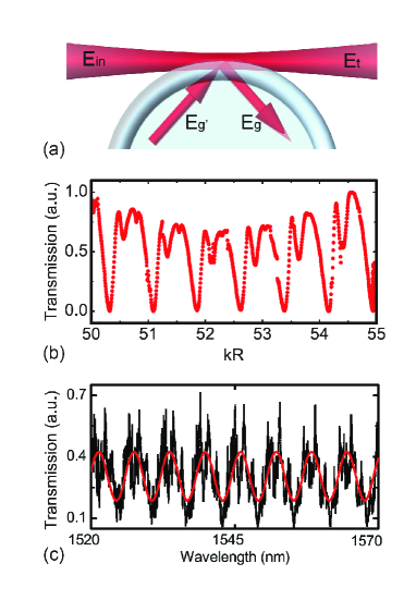
Figure 3: (Color online) (a) The schema of the scattering process described by Eq. 17. (b) Stimulated transmission spectrum of the free-space excitation process obtained by boundary element method. (c) Experimental spectrum (black) and the fitted oscillations (red).

IV On-resonance transmission

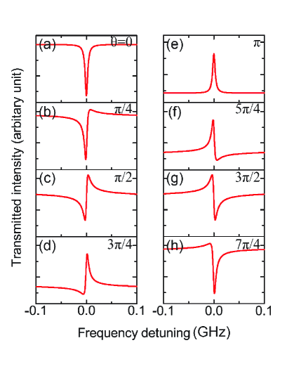
Figure 4: (a)-(h) Calculated transmission spectra with $\kappa/2\pi,\gamma/2\pi=0.003$ GHz and $t/r=0.2$. The phase shift between the two amplitudes varies from 0 to $7\pi/4$.

We turn to the study of the on-resonance transmission. It is noted that the direct excitation probability of high-Q regular modes via evanescent field is negligible due to angular momentum mismatch, so that the amplitude of $\langle\mathrm{WGM}|S|\mathrm{in}\rangle$ in Eq. (14) has minor contribution of the transmission. In this case, the lineshape parameter $q$ can be reduced to a simplified form. Substituting Eq. (19) into Eq. (14), we obtain the expression of the lineshape parameter

$$q_{\omega}=\frac{\mathrm{v.p.}\int\mathrm{d}\omega^{\prime}\frac{1}{\omega-\omega^{\prime}}V_{\omega^{\prime}}^{\ast}\langle\mathrm{C}_{\omega^{\prime}}|S|\mathrm{in}\rangle}{\pi V_{\omega}^{\ast}\langle\mathrm{C}_{\omega}|S|\mathrm{in}\rangle}=-\frac{ie^{i\theta}}{t/r+e^{i\theta}},$$ (21)

where $\theta=\mathrm{nk}L_{\mathrm{eff}}$ as mentioned above. Substituting Eq. (21) into Eq. (13), the on-resonance transmission can be deduced. In the following, we will show that the lineshape of the transmission spectrum is determined by $q_{\omega}$, which primarily depends on $\theta$, while the modulation depth relies on the relative coupling strength described by $K$.

Figures 4(a)-4(h) plot calculated transmission spectra against the phase difference $\theta$, which experience symmetric Lorentz absorption dips, asymmetric Fano-like lineshapes and symmetric electromagnetically-induced-transparency (EIT)-like peaks as $\theta$ varies from $0$ to $2\pi$. From Fig. 3(a), the transmission is a result of interference between two components: the direct transmitted light and the emitted light from the cavity, and $\theta$ actually describes the phase difference between them. Interestingly, the on-resonance transmission appears a symmetric dip on the background where the two components constructively interfere ($\theta=0$ in Fig. 4(a)), while it switches to an EIT-like peak when they destructively interfere ($\theta=\pi$ in Fig. 4(e)). This is because when on resonance, the chaotic modes refractively excited by the incident beam can couple to the regular mode via dynamical tunneling, which results in a phase shift as energy couples back to the chaotic modes. Hence, although the background components constructively (destructively) interfere, such counteraction adds a destructive modulation to the chaotic modes, reflecting a dip (peak) on the transmission.

As discussed above, the Fano-resonance transmission spectra can be regarded as the modulation of the high-Q mode on the off-resonance background. Such modulation depends strongly on the coupling strength $\kappa$ between the chaotic modes and the regular mode according to Eq. (13). Here we study the two special cases: EIT-like lineshapes and Lorentz dips. As shown in the solid curve in Fig. 5(a), the modulation of the regular mode to the transmission spectrum is minor when $K=60$. In this case, the excitation probability is extremely low. As $K$ decreases (i.e., the dynamical tunneling is enhanced), the height of the EIT peak increases monotonically, where the off-resonance backgrounds are lifted to the same level. When the loss described by $\gamma_{0}+\gamma_{1}$ is negligible compared with the coupling strength $\kappa$, ı.e., $K\rightarrow 0$, the EIT peak reaches its maximum. Similarly, Fig. 5(b) shows that the dynamical-tunneling-induced dips become more obvious by enhancing the tunneling, as expected.

V Physical meaning of the chaotic mode and ‘complete excitation’

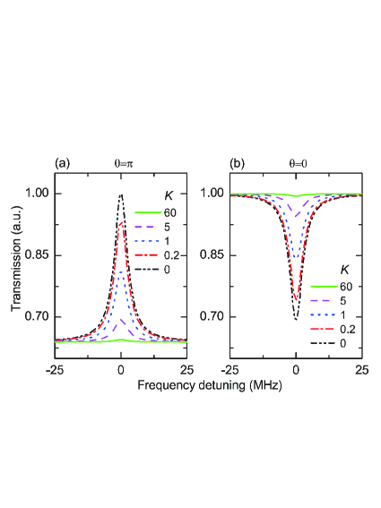
Figure 5: (Color online) Calculated transmission spectra with $\gamma_{t}/2\pi=0.006$ GHz and $t/r=0.2$, and with $K$ varying from 0 to 60, for (a) EIT-like lineshape and (b) Lorentz-like lineshape. The background is set to the same level for each graph.

At the beginning of Sec. II, we have presented the chaotic mode $\left|\mathrm{C}_{\omega}\right\rangle$. In this section, we will further investigate the meaning of the chaotic mode and the coupling strength to a regular mode $|\mathrm{WGM}\rangle$. To study this case in a general way, we expand the chaotic mode as a linear combination of an orthogonal set at a certain frequency. Using $\left|\mathrm{C}_{\omega(n)}\right\rangle$ to represent the normalized $n$-th orthogonal mode, we have

$$|\mathrm{C}_{\omega}\rangle=\frac{1}{\sqrt{\displaystyle{\sum_{n}}\alpha_{(n)}^{2}}}\displaystyle{\sum_{n}}\alpha_{(n)}|\mathrm{C}_{\omega(n)}\rangle,$$ (22)

where $\alpha_{(n)}$ stands for the corresponding weight. From the coupled mode theory, we obtain

$$\dot{\xi}_{r}=\displaystyle\sum_{n}g_{(n)}\xi_{(n)}.$$ (23)

Here $\xi_{n}$ and $\xi_{r}$ represent the electric field of $|\mathrm{C}_{\omega(n)}\rangle$ and $|\mathrm{WGM}\rangle$, respectively, with $g_{n}$ being the coupling strength between them. Thus, the equivalent coupling strength $|V_{\omega}|$ is derived as

$$|V_{\omega}|=\frac{1}{\sqrt{\displaystyle{\sum_{n}}\alpha_{(n)}^{2}}}\displaystyle{\sum_{n}}\alpha_{(n)}g_{(n)}.$$ (24)

Then the reduced coupling strength between $|\mathrm{C}_{\omega}\rangle$ and $|\mathrm{WGM}\rangle$ can be obtained as $\kappa=2\pi|V_{\omega}|^{2}$, according to Eq. (8).

Once the high-Q regular mode $|\mathrm{WGM}\rangle$ is excited, it can dynamically tunnel into all the chaotic modes including both $\left|\mathrm{C}_{\omega}\right\rangle$ and $\left|\mathrm{C}_{\omega}^{\perp}\right\rangle$. Since the chaotic modes are continuum, with first Markov approximation, this tunneling can be considered as a spontaneous decay process of the regular mode, described by the coefficient

$$\gamma_{\omega}=\sqrt{\displaystyle{\sum_{n}}g_{(n)}^{2}}.$$ (25)

Thus the decay rate into $\left|\mathrm{C}_{\omega}^{\perp}\right\rangle$ is

$$\frac{\gamma_{\mathrm{1}}}{2\pi}=\left|\gamma_{\omega}\right|^{2}-\frac{\kappa}{2\pi}=\frac{\displaystyle{\sum_{n}}\alpha_{(n)}^{2}\displaystyle{\sum_{n}}g_{(n)}^{2}-(\displaystyle{\sum_{n}}\alpha_{(n)}g_{(n)})^{2}}{\displaystyle{\sum_{n}}\alpha_{(n)}^{2}}.$$ (26)

Hence, to optimize the free-space coupling efficiency, according to Cauchy inequality, the coefficients $\alpha_{(n)}$ satisfies

$$\frac{\alpha_{(1)}}{g_{(1)}}=\frac{\alpha_{(2)}}{g_{(2)}}=\cdots=\frac{\alpha_{(n)}}{g_{(n)}}.$$ (27)

Under this condition, it is found $\gamma_{\mathrm{1}}=0$. Neglecting the intrinsic loss $\gamma_{\mathrm{0}}$ induced by scattering and material absorption, we have $\kappa=\gamma_{\mathrm{t}}$, which means the incident light is exactly a time-reversed way of the emission light from the regular mode $|\mathrm{WGM}\rangle$. It is also in agreement with the second extreme case discussed in Sec. II, that the ‘complete excitation’ condition requires the incident light as the phase conjugation wave of the emission pattern.

VI KAM barriers

Finally, we discuss how the KAM tori, behaving as barriers PRL1986 ; PRL2007 , can result in a phase shift in dynamical tunneling. This phase shift is crucial to give rise to the Fano resonance. As shown in Fig. 2(a), KAM tori separate the phase space into disconnected regions, between which transport is forbidden classically, but permitted in quantum mechanics TurnstileAn ; PRLsong , known as dynamical tunneling. To evaluate the barrier effect, we study the potential of orbits in the PSOS. For the sake of analytical expressions but without loss of the physics, we investigate the orbits in a circular microcavity. The wave function of a WGM with angular momentum number $\mathrm{m}$ in circular cavities takes the form

$$\Psi(\mathbf{r},\phi)=f_{\mathrm{m}}(\mathbf{r})e^{i\mathrm{m}\phi},$$ (28)

where $f_{\mathrm{m}}(\mathbf{r})$ satisfies the radial wave equation

$$[-\nabla_{\mathbf{r}}^{2}-\frac{(\mathrm{n}^{2}(\mathbf{r})-1)\omega^{2}}{c^{2}}+\frac{\mathrm{m}^{2}}{r^{2}}]f_{\mathrm{m}}(\mathbf{r})=\frac{\omega^{2}}{c^{2}}f_{\mathrm{m}}(\mathbf{r}).$$ (29)

Based on the stationary Schrödinger equation

$$(-\frac{\hbar^{2}}{2\mu}\nabla^{2}+V)f_{\mathrm{m}}(\mathbf{r})=Ef_{\mathrm{m}}(\mathbf{r})$$ (30)

and substituted with $E=\hbar\omega$, we deduce the effective potential corresponding to the angular momentum number $\mathrm{m}$

$$V=\frac{\hbar^{2}}{2\mu}[-\frac{(\mathrm{n}(\mathbf{r})^{2}-1)\omega^{2}}{c^{2}}+\frac{\mathrm{m}^{2}}{r^{2}}].$$ (31)

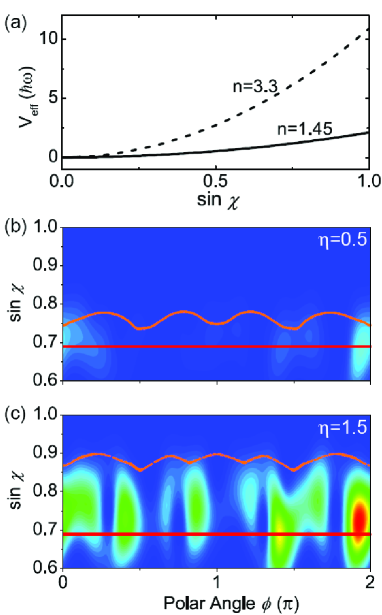
Figure 6: (Color online) (a) Effective potential $V_{\mathrm{eff}}$ against $\sin\chi$. The solid and the dashed curves correspond to the cases of silica (n=1.45) and GaAs (n=3.3) microcavities, respectively. (b)-(c) Husimi projections of the excitation state inside the cavity at non-resonant frequency with the deformation parameter $\eta$ of the cavity setting as $0.5$ and $1.5$, respectively. These two figures are plotted in the same scale. Orange dotted curves and red solid lines denote KAM tori and critical-refraction lines.

Extending $\mathrm{m}$ to the range of positive real numbers, from the classical relation $\mathrm{m}=\mathrm{nkr}\sin\chi$ and the non-relativity approximation $\mu=\hbar\omega/2c^{2}$, the effective potential of the orbits takes the form

$$V_{\mathrm{eff}}(\sin\chi)=\mathrm{n^{2}}\hbar\omega\sin^{2}\chi,$$ (32)

The effective potentials for different meterials (silica and GaAs) are plotted in Fig. 6(a). Thus, an photon at critical refraction line $\sin\chi=1/\mathrm{n}$ has the same potential as a free-space photon, in agreement with the Fresnel’s Law. The difference in the potentials of various orbits leads to tunneling.

In deformed microcavities, KAM tori are the residue of these invariant orbits, and they perform as barriers in quantum mechanics. By plotting the Humisi projection of cavities of different deformations shown in Figs. 6(b)-(c), we can find that the transportation to high-Q modes are governed by the KAM tori. Our simulation also reveals that more light can be localized in the cavity with a larger deformation, thus leading a higher probability to couple into regular high-Q modes.

VII summary

In conclusion, we have presented the dynamical tunneling-assisted coupling mechanism to interpret how a free-space laser beam excites the high-Q modes in deformed microcavities. The deformed microcavity has a mixed phase space, where the high-Q regular modes lie in regular regions. Lifetime of photons refracting into the cavity increases due to chaotic trajectories, which contributes to the enhanced excitation of regular modes via chaos-assisted dynamical tunneling. A quantum scattering theory is employed to describe the picture and to obtain the free-space transmission spectra. Unlike evanescent coupling with a waveguide where the transmission spectra behave symmetrically, this model predicts three types of transmission, i.e., asymmetric Fano-like, symmetric EIT-like and Lorentz dip lineshapes, depending on the phase difference related to the fluctuation of background transmission. It is found that the Fano resonance is attributed to the phase shift occurring in the dynamical tunneling into classical-forbidden regions. Our results provide a general method to evaluate the coupling strength between the chaos and the regular mode from the transmission spectra, which can be further extended to the quantitative study of the dynamical tunneling process. The efficient chaos-assisted free-space coupling is of importance to simplifying experimental condition and exciting high-Q modes in higher-index-material microcavities.

- (1) Optical Microcavities, edited by K. Vahala (World Scientific, Singapore, 2005).
- (2) S.-X. Qian and R. K. Chang, Phys. Rev. Lett. 56, 926 (1986).
- (3) S. M. Spillane, T. J. Kippenberg, and K. J. Vahala, Nature 415, 623 (2002).
- (4) V. S. Ilchenko, A. A. Savchenkov, A. B. Matsko, and L. Maleki, Phys. Rev. Lett. 92, 043903 (2004).
- (5) P. Del’Haye, T. Herr, E. Gavartin, M. L. Gorodetsky, R. Holzwarth, and T. J. Kippenberg, Phys. Rev. Lett. 107, 063901 (2011).
- (6) T. Aoki, B. Dayan, E. Wilcut, W. P. Bowen, A. S. Parkins, T. J. Kippenberg, K. J. Vahala, and H. J. Kimble, Nature (London) 443, 671 (2006).
- (7) Y.-S. Park, A. K. Cook, and H. Wang, Nano Lett. 6, 2075 (2006).
- (8) Y.-F. Xiao et al., Phys. Rev. A 85, 031805(R) (2012).
- (9) T. J. Kippenberg, H. Rokhsari, T. Carmon, A. Scherer, and K. J. Vahala, Phys. Rev. Lett. 95, 033901 (2005).
- (10) A. H. Safavi-Naeini, T. P. Mayer Alegre, J. Chan, M. Eichenfield, M. Winger, Q. Lin, J. T. Hill, D. E. Chang, and O. Painter, Nature 472, 69 (2011).
- (11) C. Dong, V. Fiore, M. C. Kuzyk, and Hailin Wang, Science 338, 1609 (2012).
- (12) V. Sandoghdar, F. Treussart, J. Hare, V. Lefevre-Seguin, J.-M. Raimond, and S. Haroche, Phys. Rev. A 54, R1777 (1996).
- (13) G. S. Solomon, M. Pelton, and Y. Yamamoto, Phys. Rev. Lett. 86, 3903 (2001).
- (14) L. Yang, D. K. Armani, and K. J. Vahala, Appl. Phys. Lett. 83, 825 (2003).
- (15) Y.-F. Xiao, C.-H. Dong, C.-L. Zou, Z.-F. Han, L. Yang, and G.-C. Guo, Opt. Lett. 34, 509 (2009).
- (16) F. Vollmer, D. Braun, A. Libchaber, M. Khoshsima, I. Teraoka, and S. Arnold, Appl. Phys. Lett. 80, 4057 (2002).
- (17) I. M. White, H. Oveys, and X. Fan, Opt. Lett. 31, 1319 (2006).
- (18) F. Vollmer, S. Arnold, and D. Keng, Proc. Natl. Acad. Sci. U.S.A. 105, 20701 (2008).
- (19) J. Zhu, S. K. Ozdemir, Y.-F. Xiao, L. Li, L. He, D.-R. Chen, and L. Yang, Nature Photon. 4, 46 (2010).
- (20) Y.-F. Xiao, V. Gaddam, and L. Yang, Opt. Express 16, 12538 (2008).
- (21) V. B. Braginsky, M. L. Gorodetsky, and V. S. Ilchenko, Phys. Lett. A 137, 393 (1989).
- (22) J. C. Knight, G. Cheung, F. Jacques, and T. A. Birks, Opt. Lett. 22, 1129 (1997).
- (23) M. Cai, O. Painter, and K. J. Vahala, Phys. Rev. Lett. 85, 74 (2000).
- (24) V. S. Ilchenko, X. S. Yao, and L. Maleki, Opt. Lett. 24, 723 (1999).
- (25) S.-B. Lee, J. Yang, S. Moon, J.-H. Lee, and K. An, Appl. Phys. Lett. 90, 041106 (2007).
- (26) J. Yang, S.-B. Lee, S. Moon, S.-Y. Lee, S.W. Kim, TruongThiAnh Dao, J.-H. Lee, and K. An, Phys. Rev. Lett. 104, 243601 (2010).
- (27) J. U. Nöckel and A. D. Stone, Nature 385, 45 (1997).
- (28) Y.-S. Park and H. Wang, Opt. Express 15, 16471 (2007).
- (29) U. Fano, Phys. Rev. 124, 1866 (1961).
- (30) Y.-F. Xiao et al., http://arxiv.org/abs/1209.4441.
- (31) C. L. Zou, F. W. Sun, C. H. Dong, X. W. Wu, J. M. Cui, Y. Yang, G. C. Guo, Z. F. Han, http://arxiv.org/abs/0908.3531.
- (32) X.-F. Jiang, Y.-F. Xiao, C.-L. Zou, L. He, C.-H. Dong, B.-B. Li, Y. Li, F.-W. Sun, L. Yang, and Q. Gong, Adv. Mater. 24, OP260 (2012).
- (33) V. I. Arnol’d, Russ. Math. Surv. 18, 9 (1963).
- (34) J. U. Nöckel, A. D. Stone, and R. K. Chang, Opt. Lett. 19, 1693 (1994).
- (35) C. Gmachl et al., Science 280, 1556 (1998).
- (36) M. Hentschel and K. Richter, Phys. Rev. E 66, 056207 (2002).
- (37) S.-Y. Lee and K. An, Phys. Rev. A 83, 023827 (2011).
- (38) M. Hentschel, H. Schomerus, and R. Schubert, Europhys. Lett. 62, 636 (2003).
- (39) As the regular mode lies on an invariant torus behaving much like whispering gallery mode, we use WGM to represent it.
- (40) A. Bäcker, R. Ketzmerick, S. Löck, and L. Schilling, Phys. Rev. Lett 100, 104101 (2008).
- (41) C.W. Gardiner and P. Zoller, Quantum Noise, 3rd ed. (Springer, Berlin, 2004).
- (42) H. Schomerus and M. Hentschel, Phys. Rev. Lett. 96, 243903 (2006).
- (43) J. Yang, S.-B. Lee, S. Moon, S.-Y. Lee, S. W. Kim, and K. An, Opt. Express 18, 26141 (2010).
- (44) T. Geisel, G. Radons, and J. Rubner Phys. Rev. Lett. 57, 2883 (1986).
- (45) I. I. Rypina, M. G. Brown, F. J. Beron-Vera, H. Kocak, M. J. Olascoaga, and I. A. Udovydchenkov, Phys. Rev. Lett. 98, 104102 (2007).
- (46) J.-B. Shim, S.-B. Lee, S. W. Kim, S.-Y. Lee, J. Yang, S. Moon, J.-H. Lee, and K. An, Phys. Rev. Lett. 100, 174102 (2008).
- (47) Q. Song, L. Ge, B. Redding, and H. Cao, Phys. Rev. Lett. 108, 243902 (2012).