Controlling and reversing the transition from classical diffusive
to quantum ballistic transport in a quantum walk by driving the coin

Abstract

We show that the standard quantum-walk quantum-to-classical transition, characterized by ballistic-to-diffusive spreading of the walker’s position, can be controlled by externally modulating the coin state. We illustrate by showing an oscillation between classical diffusive and quantum ballistic spreading using numerical and asymptotically exact closed-form solutions, and we prove that the walker is in a controllable incoherent mixture of classical and quantum walks with a reversible quantum-to-classical transition.

I Introduction

The quantum walk on a lattice Kempe (2003a, b) is an important branch of quantum information research for several reasons Kendon (2011). The quantum walk concept drives breakthroughs in quantum algorithms, including speeds up for quantum searches Santha (2008) and exponential speed-ups of graph traversal compared with the best known classical algorithms for such tasks Childs et al. (2003); Shenvi et al. (2003). Beyond quantum algorithms and into the physical world, quantum walks are evident in spin-chain quantum transport Kay (2010) and photosynthetic excitonic energy transport Mohseni et al. (2008). Quantum walks serve as one model for quantum computation Childs (2009); Childs et al. (2012) alongside other models such as circuit Deutsch (1985), measurement-based Raussendorf and Briegel (2001), adiabatic Farhi et al. (2001) and topological quantum computing Nayak et al. (2008). Experimental realizations of quantum walks abound with successes having been reported in nuclear magnetic resonance Ryan et al. (2005), ion traps Zähringer et al. (2010) and photons Broome et al. (2010); Schreiber et al. (2011).

Decoherence is especially important in quantum walk implementations, both because it deleteriously destroys unitarity with consequences such as transforming the ballistic spreading to diffusive spreading Brun et al. (2003a, b); Kendon and Sanders (2005) and because of the beneficial property of enabling tuning of quantum walk dynamics Kendon (2007). Typically decoherence is characterized by the rate of spreading of the walker’s position after tracing over the coin state, and ballistic spreading is ‘quantum’ and diffusive spreading is ‘classical’.

Here we show that controlling the walker’s coin in an appropriate time-dependent way enables the walker to achieve diffusive spreading and later back to ballistic, i.e. transferring between classical and quantum behavior in a controlled way. Our result is distinct from studies of recurrences in quantum-walk dynamics Štefaňák et al. (2008) and from unitarily controlled “stroboscopic” quantum walks Buerschaper and Burnett (2004) or, equivalently, modified quantum walk dynamics by periodic perturbations Wójcik et al. (2004). Those investigations are essentially about unitary control.

Our result, based on controlled non-unitary evolution through coin measurements, instead challenges the paradigm of the irreversibility of the ballistic-to-diffusive spreading rate due to coin measurement. On the other hand we show that the sacrosanct principle of non-decreasing walker-distribution entropy remains intact.

II Formalism

The joint walker-coin state $\rho_{\text{wc}}$ is a trace-class positive operator on the Hilbert space $\mathscr{H}=\mathscr{H}_{\text{w}}\otimes\mathscr{H}_{\text{c}}$ such that $\mathscr{H}_{\text{w}}=\text{span}\{|x\rangle;x\in\mathbb{Z}\}$ with $|x\rangle$ the orthonormal walker position states on a regular integer lattice, and $\mathscr{H}_{\text{c}}=\text{span}\{|\pm\rangle\}$ with $|\pm\rangle$ the two coin states. If the walker-coin system undergoes periodic unitary steps, the evolution operator is given by

$$U:=F(\mathds{1}\otimes C)$$ (1)

for $\mathds{1}$ the identity, $H$ the Hadamard operator,

$$C:=H=\frac{1}{\sqrt{2}}\begin{pmatrix}1&1\\ 1&-1\end{pmatrix},$$ (2)

and

$$F:=S\otimes\left|{+}\right\rangle\left\langle{+}\right|+S^{\dagger}\otimes\left|{-}\right\rangle\left\langle{-}\right|$$ (3)

the conditional shift operator with shift operator

$$S:=\sum_{x}\left|{x+1}\right\rangle\left\langle{x}\right|.$$ (4)

The walker’s evolving state is

$$\rho_{\text{wc}}(t)=\mathcal{U}^{t}\rho_{\text{wc}}(0):=(U^{\dagger})^{t}\rho_{\text{wc}}(0)U^{t}$$ (5)

for discrete time parameter $t\in\mathbb{Z}$. The driven-coin case is more complicated and treated below.

We now generalize for the case of the driven coin. Prior to each unitary coin ‘flip’, a completely-positive trace-preserving map $\mathcal{E}(t,0):\rho_{\text{c}}(0)\mapsto\rho_{\text{c}}(t)$ is applied to the coin. The map can be decomposed into the operator sum

$$\mathcal{E}\rho_{\text{c}}=\sum_{n\in\{0,\pm\}}A_{n}\rho_{\text{c}}A^{\dagger}_{n}$$ (6)

such that

$$\sum_{n\in\{0,\pm\}}A^{\dagger}_{n}A_{n}=\mathds{1}$$ (7)

with

$$A_{0}=\sqrt{\kappa(t)}\mathds{1},\;A_{\pm}=\sqrt{1-\kappa(t)}\mathcal{P}^{\pm},$$ (8)

and

$$\mathcal{P}^{\pm}=\left|{\pm}\right\rangle\left\langle{\pm}\right|,$$ (9)

emerge corresponding to a coin with probability $1-\kappa$ of being measured at each step. In other words, $\kappa(t)$ is effectively a time-varying strength of coin-state measurement.

To understand the time-varying strength of the measurement, let us consider a distinct but easy-to-undersand ‘off-on-off’ model, where $\kappa=1$ (no measurement hence perfect quantum walk) for some time, then zero (strongest possible measurement, which reduces the dynamics to a classical random walk), then unity (i.e., back to the quantum walk) again. When the coin is unmeasured during the ‘off’ interval, no dephasing takes place; hence the quantum walk is unitary and the walker-coin state is an entangled pure state.

Now consider the second interval of this ‘off-on-off’ model. During this time the entangled pure state is subject to a strong coin-state measurement in the $|\pm\rangle$ basis. Our unconditional measurement erases the knowledge of whether $+$ or $-$ were read and instead projects the entangled state into a mixture of two product states of the walker with the coin state: $|\phi_{\pm}\rangle|\pm\rangle$. This state corresponds to whether the walker’s motion is in the $+$ or $-$ direction in the last step Kendon and Sanders (2005).

If the measurement were now turned off permanently, each of these states would evolve according to the quantum walk. Although mixing would appear to erase some of the finer interference fringes, both pure states would result in ballistic spreading of the walker. If the strong measurement is on for two time steps, four pure states $|\phi_{+\pm}\rangle|\pm\rangle$ and $|\phi_{-\pm}\rangle|\pm\rangle$ corresponding to the four measurement outcomes. Our unconditional measurement model loses knowledge of the two coin measurements and thereby yields a mixture of these four states and a narrow spread than for each walker distribution individually because of regression to the classical walk. Furthermore these states then evolve to produce ballistic spreading of the walker’s position.

We have considered just two time steps of strong measurement. Now consider extrapolating to many times steps corresponding to many sequential strong measurements. The consequence of this measurement taking place over $t$ times steps is exponentially many (in terms of $t$) pure states all blended together in one mixed state. This mixed state converges to a Gaussian walker whose position spread reaches classical-walk width. Then, when the strong measurement ceases after $t$ steps, ballistic spreading recommences for each element of the mixture hence the walker’s distribution as a whole.

This ‘off-on-off’ model shows how sequential strong and weak measurements affect the dynamics at an intuitive level, but having the walker position distribution alternately increase and decrease over time requires a more sophisticated model. As we show in the next section, the ‘periodically varying measurement strength’ model delivers such a result.

III Periodically varying measurement strength

In this section, we introduce the ‘periodically varying measurement strength’ model and begin by analyzing numerically the effect of periodically varying the coin measurement strength. Specifically we are concerned with the dynamically changing reduced walker position distribution, and the time-dependent variance and entropy associated with this distribution. For the periodic dynamical map with

$$\kappa(t)=\cos\eta t,$$ (10)

the corresponding state mapping is

$$\mathcal{E}\rho_{\text{c}}=\kappa(t)\rho_{\text{c}}+[1-\kappa(t)]\left[\mathcal{P}^{+}\rho_{\text{c}}\mathcal{P}^{+}+\mathcal{P}^{-}\rho_{\text{c}}\mathcal{P}^{-}\right]$$ (11)

and

$$\rho_{\text{c}}^{00}\mapsto \rho_{\text{c}}^{00},\rho_{\text{c}}^{01}\mapsto\cos\eta t\rho_{\text{c}}^{01},$$

$$\rho_{\text{c}}^{10}\mapsto \cos\eta t\rho_{\text{c}}^{10},\rho_{\text{c}}^{11}\mapsto\rho_{\text{c}}^{11}.$$

The walker’s reduced state and resultant position distribution at time $t$ are

$$\rho_{\text{w}}(t)=\text{Tr}_{\text{c}}\rho_{\text{wc}}(t)$$ (12)

with

$$P_{\text{w}}(x,t)=\langle x|\rho_{\text{w}}(t)|x\rangle$$ (13)

respectively.

If the coin state is initially

$$\frac{\left|{+}\right\rangle+i\left|{-}\right\rangle}{\sqrt{2}}$$ (14)

and $P_{\text{w}}(x,0)=\delta_{x0}$, then $P_{\text{w}}(x,t)=P_{\text{w}}(-x,t)$. The walker’s spread is

$$\sigma(t):=\sqrt{V(t)},\;V=\langle x^{2}\rangle-\langle x\rangle^{2}$$ (15)

and $\langle x^{m}\rangle(t)$ the $m^{\text{th}}$ moment of $P_{\text{w}}(x,t)$. Rate of spreading $\sigma(t)$ is widely used to differentiate between quantum and classical random walks. In diffusive transport, $V\propto t$, whereas $V\propto t^{2}$ for ballistic transport, which holds for the coherent quantum walk Ahlbrecht et al. (2011, 2012).

Driving the coin with periodic $\kappa(t)$ affects variance $V$ as shown in Fig 1(a):

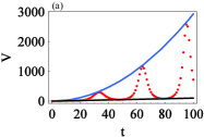
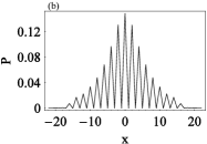
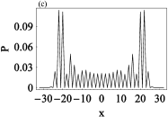
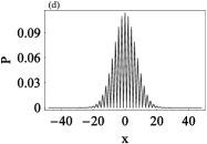
Figure 1: (Color online) (a) Numerically evaluated variance of the walker’s position over time $t$ with initial state $\left|{0}\right\rangle(\left|{+}\right\rangle+i\left|{-}\right\rangle)/\sqrt{2}$: unitary evolution (blue solid), driving with $\kappa(t)=\cos t/10$ (red dot), and random walk (black solid). Position distribution $P$ at (b) $t=22$, (c) $t=32$, and (d) $t=48$.

$V$ oscillates periodically between classical diffusive and quantum ballistic values at various times $t$ with an $\eta$-dependent period as anticipated by the above argument. Variances of the undriven-coin quantum walk and the classical random walk provide tight upper and lower bounds for the driven-coin time-dependent variance. Figures 1(b-d) display numerical results for the position distribution as a blend of classical and quantum distributions ($t=22$), nearly fully quantum ($t=32$) and nearly fully classical ($t=48$).

As Figs. 1(a-d) are shown for just one frequency $\eta$ of the driving field, we show the generality of our result for a periodic driving field by repeating for two other higher frequencies. The corresponding variance functions are shown in Figs. 2(a,b), and the periodic oscillation of $V$ is evident in these plots as well.

(a) (b)

Figure 2: (Color online) Numerically evaluated variance of the walker s position over time $t$ with same the same initial state as in Fig, 1 but driving with (a) $\kappa(t)=\cos t/2$ and (b) $\kappa(t)=\cos 3t/10$.

For generality we also consider a non-sinusoidal driving function. Specifically we consider the sawtooth driving function depicted in Fig. 3(a)

(a) (b)

Figure 3: (Color online) (a) The sawtooth driving function $\kappa(t)$ and (b) the corresponding numerically evaluated variance of the walker s position as a function of time $t$.

and show the corresponding time-dependent variance in Fig. 3(b), which also shows the periodicity of the variance over time, commensurate with the periodicity observed for the sinusoidal driving function.

The decreasing variance at times can seem counter-intuitive. The variance is often closely associated with a distribution’s entropy, especially for the normal distribution. As our control is an incoherent measurement process, the decreasing variance is startling unless the concepts of variance and entropy are dissociated. We now show that the entropy of the walker’s position distribution is non-decreasing despite the variance decreasing.

The randomness in the system is reflected in the position of the walker.

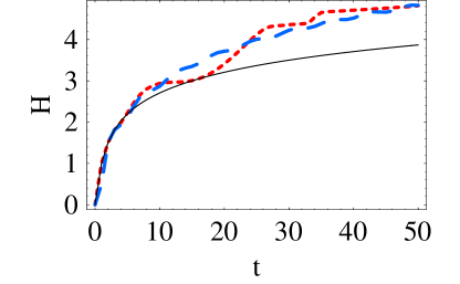
Figure 4: (Color online) Numerically evaluated entropy $H$ of the walker over time $t$ with initial state $\left|{0}\right\rangle(\left|{+}\right\rangle+i\left|{-}\right\rangle)/\sqrt{2}$: unitary evolution (blue dash), driving with $\kappa(t)=\cos(t/10)$ (red dot), and random walk (black solid).

We employ the entropy

$$H(t)=-\sum_{x}P_{\text{w}}(x,t)\text{log}_{2}P_{\text{w}}(x,t)$$ (16)

to characterize the randomness of the walker system. We plot the entropies for a classical RW, QW with unitary evolution and QW with a driven coin in Fig. 4. From the numerical simulations we can see that, for these three kinds of walks, the entropies which represent randomness are increasing with time. Though the periodically driven coin measurement causes the variance to increase and to decrease alternately over time, the randomness of the walker’s position position distribution, quantified by entropy (16), never decreases.

IV Asymptotic analysis with the ‘momentum’ representation

Using ‘momentum’ states in the Fourier domain

$$\left|{k}\right\rangle=\sum_{x=-\infty}^{\infty}\text{e}^{ikx}\left|{x}\right\rangle$$ (17)

such that

$$S\left|{k}\right\rangle=\text{e}^{-ik}\left|{k}\right\rangle,\;k\in\mathbb{R},$$ (18)

in whose basis the evolution is given by

$$U\left|{k}\right\rangle_{\text{w}}\otimes\left|{\Phi}\right\rangle_{\text{c}}=\left|{k}\right\rangle\otimes U(k)\left|{\Phi}\right\rangle_{\text{c}}$$ (19)

for

$$U(k)=\frac{1}{\sqrt{2}}\begin{pmatrix}\text{e}^{-ik}&\text{e}^{-ik}\\ \text{e}^{ik}&-\text{e}^{ik}\end{pmatrix}.$$ (20)

If the initial walker-coin state corresponds to the walker localized at the origin $x=0$ and the coin in any pure state $|\Phi\rangle_{\text{c}}$, the inverse transform expression

$$\left|{x}\right\rangle=\int^{\pi}_{-\pi}\not{\text{d}}k\text{e}^{-ikx}\left|{k}\right\rangle$$ (21)

(for $\not{\text{d}}k:=\frac{\text{d}k}{2\pi}$) yields the $t$-dependent joint walker-coin state

$$\rho(t)=\int_{-\pi}^{\pi}\not{\text{d}}k\int_{-\pi}^{\pi}\not{\text{d}}k^{\prime}\left|{k}\right\rangle\left\langle{k^{\prime}}\right|\otimes U^{t}(k)\rho_{c}(U^{\dagger}(k))^{t}.$$ (22)

After $t$ steps the state is

$$\rho_{\text{wc}}\left(t\right)=\int\not{\text{d}}k\int\not{\text{d}}k^{\prime}\left|{k}\right\rangle\left\langle{k^{\prime}}\right|\otimes\mathcal{L}^{t}(k,k^{\prime})\rho_{\text{c}}$$ (23)

for

$$\mathcal{L}(k,k^{\prime})\hat{O}:=\sum_{i\in\{0,\pm\}}U(k)A_{i}\hat{O}A^{\dagger}_{i}U^{\dagger}(k^{\prime}).$$ (24)

For $k=k^{\prime}$ this superoperator satisfies

$$\text{Tr}[\mathcal{L}^{t}(k,k)\hat{O}]=\text{Tr}[\hat{O}]$$ (25)

for any $\hat{O}$ so $\mathcal{L}(k,k)$ is trace-preserving.

Figure 1 is derived numerically hence not conclusive in revealing asymptotic spreading behavior arising from the periodically driven coin. Therefore, we exploit the momentum representation to derive the asymptotic long-time position distribution

$$P_{\text{w}}(x;t)=\int_{-\pi}^{\pi}\not{\text{d}}k\int_{-\pi}^{\pi}\not{\text{d}}k\text{e}^{-i(k-k^{\prime})x}\text{Tr}\left[\mathcal{L}^{t}(k,k^{\prime})\rho_{c}\right]$$ (26)

of the driven-coin quantum walker. Using

$$\sum_{x=-\infty}^{\infty}x^{m}\exp[-ix(k-k^{\prime})]=2\pi(-i)^{m}\delta^{(m)}(k-k^{\prime}),$$ (27)

we obtain

$$\left\langle\hat{x}^{m}\right\rangle=(-1)^{m}\int_{-\pi}^{\pi}\not{\text{d}}k\int_{-\pi}^{\pi}\not{\text{d}}k^{\prime}\delta^{(m)}(k-k^{\prime})\text{Tr}\{\mathcal{L}^{t}(k,k^{\prime})\rho_{c}\}$$

so the first two moments are

$$\left\langle\hat{x}\right\rangle=-\int_{-\pi}^{\pi}\not{\text{d}}k\sum_{j=1}^{t}\text{Tr}\{Z\mathcal{L}^{j}(k,k)\rho_{c}\}.$$ (28)

and

$$\left\langle\hat{x}^{2}\right\rangle= -\int_{-\pi}^{\pi}\not{\text{d}}k\Big{(}\sum_{j=1}^{t}\sum_{j^{\prime}=1}^{j}\text{Tr}\left\{Z\mathcal{L}^{j-j^{\prime}}(k,k)Z\mathcal{L}^{j^{\prime}}(k,k)\rho_{c}\right\}$$

$$+\sum_{j=1}^{t}\sum_{j^{\prime}=1}^{j-1}\text{Tr}\left\{Z\mathcal{L}^{j-j^{\prime}}(k,k)\mathcal{L}^{j^{\prime}}(k,k)\rho_{c}Z\right\}\Big{)}$$ (29)

with $Z=\begin{pmatrix}1&0\\ 0&-1\end{pmatrix}$.

As $\mathcal{L}(k,k)$ is additive, we obtain

$$\mathcal{L}(k,k)\mathcal{E}\rho_{\text{c}}= \kappa(t)\mathcal{L}(k,k)\rho_{\text{c}}$$

$$+[1-\kappa(t)]\mathcal{L}(k,k)\sum_{\epsilon\in\pm}\mathcal{P}^{\epsilon}\rho_{\text{c}}\mathcal{P}^{\epsilon}$$ (30)

with the first term on the right-hand side corresponding to a quantum-walk mapping (these terms are indicated by superscript Q) for a time-dependent coin and the second term corresponding to coherence-destroying measurements that transform the quantum walk into the random walk (these terms are indicated by a superscript R). Now we exploit linearity to find asymptotic solutions to the first and second term separately.

To study the first term on the right-hand side of (IV), we first specialize to the unitary case

$$\mathcal{L}(k,k)\hat{O}=U(k)\hat{O}U^{\dagger}(k)$$ (31)

and express

$$\left|{\Phi}\right\rangle_{\text{c}}=\sum_{l=0}^{1}c_{l}(k)\left|{\phi_{l}(k)}\right\rangle.$$ (32)

Here $\{\left|{\phi_{l}(k)}\right\rangle\}$ is the orthonormal eigenbasis for $U(k)$ with eigenvalues $\{\text{e}^{i\theta_{l}(k)}\}$ such that

$$\theta_{0}(k)+\theta_{1}(k)=\pi.$$ (33)

For the standard quantum walk with a Hadamard coin,

$$\left|{\phi_{l}(k)}\right\rangle= \sqrt{1+\cos^{2}k-(-1)^{l}\cos k\sqrt{1+\cos^{2}k}}$$

$$\times\begin{pmatrix}\text{e}^{-ik}/\sqrt{2}\\ \text{e}^{-i\theta_{l}(k)}-\text{e}^{-ik}/\sqrt{2}\end{pmatrix}.$$ (34)

Defining

$$c_{ll^{\prime}}(k):=c^{*}_{l}(k)c_{l^{\prime}}(k)$$ (35)

and

$$\theta_{l^{\prime}l}(k):=\theta_{l^{\prime}}(k)-\theta_{l}(k),$$ (36)

the coin state

$$\rho_{\text{c}}(t)=\sum_{ll^{\prime}}c_{ll^{\prime}}(k)\left|{\phi_{l^{\prime}}(k)}\right\rangle\left\langle{\phi_{l}(k)}\right|\text{e}^{i\theta_{l^{\prime}l}(k)t}$$ (37)

after $t$ steps is substituted into Eqs. (28) and (IV) to yield

$$\left\langle\hat{x}\right\rangle^{\text{Q}}=t-2\int_{-\pi}^{\pi}\not{\text{d}}k\sum_{l,l^{\prime}}c_{ll^{\prime}}(k)\mathcal{P}^{+}_{ll^{\prime}}(k)\sum_{j=1}^{t}\text{e}^{ij\theta_{l^{\prime}l}(k)}$$ (38)

with $\mathcal{P}^{+}_{ll^{\prime}}(k)=\left\langle{\phi_{l}(k)}\right|\mathcal{P}^{+}\left|{\phi_{l^{\prime}}(k)}\right\rangle$ and

$$\left\langle\hat{x}^{2}\right\rangle^{\text{Q}}= \int_{-\pi}^{\pi}\not{\text{d}}k\sum_{l,l^{\prime},l^{\prime\prime}}c_{ll^{\prime}}(k)Z_{ll^{\prime\prime}}(k)Z_{l^{\prime\prime}l^{\prime}}(k)$$

$$\times\sum_{j,j^{\prime}=1}^{t}\text{e}^{i(j-j^{\prime})^{\prime}\theta_{l^{\prime}l}(k)}$$ (39)

with $Z_{ll^{\prime}}(k)=\left\langle{\phi_{l}(k)}\right|Z\left|{\phi_{l^{\prime}}(k)}\right\rangle$.

As $U(k)$ is nondegenerate so $\theta_{0,1}(k)$ are distinct, most terms for $\left\langle\hat{x}\right\rangle^{\text{Q}}$ and $\left\langle\hat{x}^{2}\right\rangle^{\text{Q}}$ above oscillate strongly, and only diagonal terms survive in the long-time limit. For $\langle\hat{x}\rangle^{\text{Q}}$, the condition to be on the diagonal should be $l=l^{\prime}$. Whereas for $\langle\hat{x}^{2}\rangle^{\text{Q}}$ there are two sets of non-oscillatory terms: terms with $l=l^{\prime}=l^{\prime\prime}$ (for quadratic dependence on $t$) and terms with $j=j^{\prime}$ and $l=l^{\prime}$ (for linear dependence on $t$).

Inserting Eq. (IV) into the equations above yields

$$\text{V}^{\text{Q}}\longrightarrow_{t\rightarrow\infty}t^{2}(C_{2}-C_{1}^{2})$$ (40)

and

$$C_{1}= 1-2\int^{\pi}_{-\pi}\not{\text{d}}k\sum_{l=1,2}|c_{l}(k)|^{2}P^{+}_{ll}(k)=1-\int_{-\pi}^{\pi}\frac{\not{\text{d}}k}{1+\cos^{2}k}=1-\frac{1}{\sqrt{2}},$$

$$C_{2}= 1-4\int^{\pi}_{-\pi}\not{\text{d}}k\sum_{l=1,2}|c_{l}(k)|^{2}P^{+}_{ll}(k)P^{-}_{ll}(k)=1-\int_{-\pi}^{\pi}\frac{\not{\text{d}}k}{1+\cos^{2}k}=1-\frac{1}{\sqrt{2}}.$$ (41)

By path integration Nayak and Vishwanath (2000),

$$P^{\text{Q}}_{\text{w}}(x,t)\approx \int_{-\pi}^{\pi}\not{\text{d}}k\int_{-\pi}^{\pi}\not{\text{d}}k^{\prime}\text{e}^{-ix(k-k^{\prime})}\sum_{l,l^{\prime}}c^{*}_{l}(k)c_{l^{\prime}}(k^{\prime})\text{e}^{-i\left[\theta_{l^{\prime}}(k^{\prime})-\theta_{l}(k)\right]t}\left\langle{\phi_{l}(k)}\right|\phi_{l^{\prime}}(k^{\prime})\rangle$$

$$\approx \int_{-\pi}^{\pi}\text{d}k\frac{1+(-1)^{x+t}}{\pi t\frac{\sin k}{(1+\cos^{2}k)^{3/2}}}\Bigg{\{}\left(1-\frac{x}{t}\right)^{2}\cos^{2}\Bigg{[}\arcsin\left(\frac{\sin k}{\sqrt{2}}\right)t+xk-\frac{\pi}{4}\Bigg{]}$$

$$+\left[1-\left(\frac{x}{t}\right)^{2}\right]\cos^{2}\Bigg{[}\arcsin\left(\frac{\sin k}{\sqrt{2}}\right)t+(x-1)k-\frac{\pi}{4}\Bigg{]}\Bigg{\}},$$

and we now have the solution for the quantum part of the walk.

Now we proceed to study the second (random-walk) term of Eq. (IV). Using the representation

$$\hat{O}=r_{1}\mathds{1}+r_{2}X+r_{3}Y+r_{4}Z$$ (42)

(Pauli representation) Brun et al. (2003a), we obtain

$$\mathcal{L}(k,k)\hat{O}=\begin{pmatrix}1&0&0&0\\ 0&0&0&\cos 2k\\ 0&0&0&-\sin 2k\\ 0&0&0&0\end{pmatrix}\begin{pmatrix}r_{1}\\ r_{2}\\ r_{3}\\ r_{4}\end{pmatrix},$$ (43)

which leads to new expressions for the first two moments

$$\left\langle\hat{x}\right\rangle^{\text{R}}= -\int_{-\pi}^{\pi}\not{\text{d}}k\begin{pmatrix}0&0&0&1\end{pmatrix}\left(\sum_{j=1}^{t}\mathcal{L}^{j}(k,k)\right)\begin{pmatrix}r_{1}\\ r_{2}\\ r_{3}\\ r_{4}\end{pmatrix}$$

$$= 0$$ (44)

and

$$\left\langle\hat{x}^{2}\right\rangle^{\text{R}}= t-\int_{-\pi}^{\pi}\not{\text{d}}k\begin{pmatrix}1&0&0&0\end{pmatrix}\Bigg{[}Z_{L}\sum_{j=1}^{t}\sum_{j^{\prime}=1}^{j-1}\mathcal{L}^{j-j^{\prime}}(k,k)$$

$$\times\left(Z_{\text{L}}+Z_{\text{R}}\right)\mathcal{L}^{j^{\prime}}(k,k)\Bigg{]}\begin{pmatrix}r_{1}\\ r_{2}\\ r_{3}\\ r_{4}\end{pmatrix}=t$$ (45)

for

$$Z_{\text{L}}=\begin{pmatrix}0&0&0&1\\ 0&0&i&0\\ 0&-i&0&0\\ 1&0&0&0\end{pmatrix},Z_{\text{R}}=\begin{pmatrix}0&0&0&1\\ 0&0&-i&0\\ 0&i&0&0\\ 1&0&0&0\end{pmatrix}.$$ (46)

As $\left\langle\hat{x}\right\rangle^{\text{R}}=0$, $\left\langle\hat{x}^{2}\right\rangle^{\text{R}}$ equals the variance and is purely diffusive due to its proportionally with $t$.

The asymptotic binomial random-walk position distribution evaluated only over even (odd) $x$ for even (odd) $t$ is thus

$$P^{\text{R}}_{\text{w}}(x,t)=\frac{1}{2^{t}}\frac{t!}{\left[\frac{t-x}{2}\right]!\left[\frac{t+x}{2}\right]!}.$$ (47)

Thus, for a QW with a driven coin, we have the asymptotic position distribution

$$P_{\text{w}}(x,t)=\kappa P^{\text{Q}}_{\text{w}}(x,t)+(1-\kappa)P^{\text{R}}_{\text{w}}(x,t)$$ (48)

and variance

$$\text{V}=\kappa\text{V}^{\text{Q}}+(1-\kappa)t.$$ (49)

Excellent agreement between analytical asymptotic expressions and numerical results in the long-time limit is obtained, e.g. for the walker’s position distribution (Figure 5).

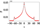
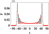
Figure 5: (Color online) Walker position distributions $P_{\text{w}}(x,t)$ for even values of $x$ and (a) $t=90$ and (b) $t=94$ with initial state $\left|{0}\right\rangle(\left|{+}\right\rangle+i\left|{-}\right\rangle)/\sqrt{2}$ and driven-coin function $\kappa(t)=\cos(t/10)$ for precise numerical simulations (dots) and asymptotic expression (solid).

V Entanglement between the walker and the coin

Although the usual signature of the quantum walk is the rate of spreading $V$, which, for the driven coin, is a weighted sum of the quantum ballistic spread $V^{\text{Q}}$ and the diffusive term $V^{\text{R}}$ proportional to $t$, the quantum-classical divide can be explored in more depth through studying entanglement between the walker and the coin. Entanglement should be zero in the random-walk case and should generally be non-zero in the quantum-walk case. We analyze walker-coin quantum correlation with two measures: measurement induced disturbance (MID) Luo (2008) and quantum discord (QD) Ollivier and Zurek (2001).

Discord uses von Neumann measurements to quantify QD Ollivier and Zurek (2001), which consist of one-dimensional projectors summing to the identity operator. We use projection operators $\{B_{j}\}$ to denote a von Neumann measurements for coin state only. Quantum conditional entropy is $S[\rho_{\text{wc}}(t)|\{B_{j}\}]:=\sum_{j}p_{j}S[\rho_{j}(t)]$ with $S(\cdot)$ the von Neumann entropy, and the associated quantum mutual information is

$$\mathcal{I}[\rho_{\text{wc}}(t)|\{B_{j}\}]:=S[\rho_{\text{w}}(t)]-S[\rho_{\text{wc}}(t)|\{B_{j}\}],$$ (50)

where the conditional density operator operator $\rho_{j}(t)=(\mathds{1}\otimes B_{j})\rho_{\text{wc}}(t)(\mathds{1}\otimes B_{j})$ with the measurement result $j$, and the probability $p_{j}=\text{Tr}[(\mathds{1}\otimes B_{j})\rho_{\text{wc}}(t)(\mathds{1}\otimes B_{j})]$.

For classical correlations

$$\mathcal{C}_{\text{cl}}[\rho_{\text{wc}}(t)]:=\text{sup}_{B_{j}}\mathcal{I}[\rho_{\text{wc}}(t)|\{B_{j}\}],$$ (51)

QD is

$$D:=\mathcal{I}[\rho_{\text{wc}}(t)]-\mathcal{C}_{\text{cl}}[\rho_{\text{wc}}(t)].$$ (52)

With respect to QD, correlations between $\rho_{\text{w}}$ and $\rho_{\text{c}}$ are classical if there exists a unique local measurement strategy on the coin $\{B_{j}\}$ leaving $\rho_{i}(t)$ unaltered from the original joint walker-coin state $\rho_{\text{wc}}(t)$. Calculating QD is difficult due the need to maximize over all possible von Neumann-type measurements of the coin state in order to determine the classical correlation.

MID Luo (2008)

$$Q[\rho_{\text{wc}}(t)]:=\mathcal{I}[\rho_{\text{wc}}(t)]-\mathcal{I}[\rho_{\text{wc}}(t)|\{B_{j}\}]$$ (53)

has an advantage over QD in that MID is operational but tends to overestimate non-classicality because of a lack of optimization over local measurements. We therefore ascertain whether the joint walker-coin state is ‘quantum’ by determining if a local measurement strategy exists that leaves the state unchanged. We numerically evaluate MID and QD for a QW in the undriven, driven-coin and random-walk cases and display results in Figure 6.

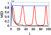
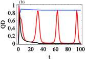
Figure 6: (Color online) (a) The MID and (b) QD for a QW on a line after $t=100$ steps for undriven (blue), driven with $\kappa(t)=\cos(t/10)$ (red) and random walk (black) cases with initial state $\left|{0}\right\rangle(\left|{+}\right\rangle+i\left|{-}\right\rangle)/\sqrt{2}$.

For the undriven-coin case, MID and QD are the same. For the driven-coin case, MID and QD exhibit quantum-correlation oscillations with the same period as for the position-variance oscillation, i.e. the oscillation between diffusive and ballistic spreading.

VI Conclusion

In summary we study the driven-coin quantum walk and discover that controlling the quantum coin causes the walker’s spread to oscillate between diffusive and ballistic spreading, which are standard signatures of classical random vs. quantum walks, respectively. Our results are determined by numerical means for all times and by closed-form expressions in the asymptotically long-time limit. We prove that the walker’s reduced position distribution is an incoherent mixture of classical- and quantum-walk distributions.

This oscillation between classical-diffusive and quantum-ballistic spreading is manifest in the quantum correlations between the walker and the coin. One can understand the surprising result of alternating increasing-decreasing variance as being due to a periodic restoration of a highly non-Gaussian walker position distribution, due to quantum walking, into a Gaussian distribution, with a concomitant decrease of variance. We show, however, that this decrease of variance is not accompanied by a decrease in entropy: entropy is strictly non-decreasing as expected for an unconditional measurement-based control. Our alternating increasing-decreasing walker-position variance results could be valuable for tuning quantum walks Kendon (2007) and especially challenge common notions of decoherence in quantum walks associated with tying variance to decoherence.