Effect of electron heating on self-induced transparency in relativistic intensity laser-plasma interaction

Abstract

The effective increase of the critical density associated with the interaction of relativistically intense laser pulses with overcritical plasmas, known as self-induced transparency, is revisited for the case of circular polarization. A comparison of particle-in-cell simulations to the predictions of a relativistic cold-fluid model for the transparency threshold demonstrates that kinetic effects, such as electron heating, can lead to a substantial increase of the effective critical density compared to cold-fluid theory. These results are interpreted by a study of separatrices in the single-electron phase space corresponding to dynamics in the stationary fields predicted by the cold-fluid model. It is shown that perturbations due to electron heating exceeding a certain finite threshold can force electrons to escape into the vacuum, leading to laser pulse propagation. The modification of the transparency threshold is linked to the temporal pulse profile, through its effect on electron heating.

I Introduction

The optical properties of a plasma under the action of a relativistically intense laser pulse (intensity $\mathrm{I}\gtrsim 10^{18}\,\mathrm{W\,cm^{-2}}$ for $1\,\mathrm{\mu m}$ wavelength) are profoundly affected by nonlinearities in the corresponding laser-plasma interaction. In particular, the question of whether a pulse with the carrier frequency $\omega_{L}$ propagates in a plasma of electron density $n_{0}$ can no longer be answered solely in terms of the critical density,

$$n_{c}=\epsilon_{0}\,m_{e}\,\omega_{L}^{2}/e^{2}\,,$$ (1)

where $m_{e}$ is the electron rest mass, $-e$ is the electron charge, and $\epsilon_{0}$ is the permittivity of free space. By definition, a relativistically intense pulse accelerates electrons from rest to relativistic momenta within an optical cycle and, thus, the electron mass in Eq. (1) has to be corrected by the relativistic factor $\gamma=\sqrt{1+\mathbf{p}^{2}/m_{e}^{2}c^{2}}$, where $\mathbf{p}$ is the electron momentum. For a purely transverse wave propagating through a cold, homogeneous plasma, this relativistic factor can be related, by the conservation of canonical momentum, to the normalized amplitude of the wave vector potential $a_{0}=eA_{0}/(m_{e}c)$, $\gamma\simeq\sqrt{1+a_{0}^{2}/2}$ . Therefore, one is forced to introduce an intensity-dependent effective critical density Akhiezer and Polovin (1956); Kaw and Dawson (1970)

$$n_{c}^{\mathrm{eff}}=\sqrt{1+\frac{a_{0}^{2}}{2}}\,n_{c}\,.$$ (2)

According to Eq. (2), a relativistically intense laser pulse ($a_{0}\gtrsim 1$) can propagate through a nominally overdense plasma, with electron density $n_{c}<n_{e}<n_{c}^{\mathrm{eff}}$, a phenomenon known as relativistic self-induced transparency (RSIT). Apart from its role as a fundamental process in laser-plasma interaction, RSIT is also interesting for applications, as it often determines the regime of efficient laser-target interaction. In the context of ion acceleration, for instance, RSIT can prevent efficient ion radiation-pressure-acceleration from thin targets Klimo et al. (2008); Robinson et al. (2008); Yan et al. (2008); Macchi et al. (2009); Grech et al. (2011) or laser-driven hole-boring in thicker ones Naumova et al. (2009); Schlegel et al. (2009). On the other hand, RSIT may enhance electron heating in the break-out afterburner acceleration mechanism, thus allowing for higher ion energies Yin et al. (2006); Albright et al. (2007); Yin et al. (2011).

In this paper, we investigate RSIT in the case of a circularly polarized (CP) laser pulse with finite rise (or ramp-up) time $\tau_{r}$ and infinite duration, normally incident onto a semi-infinite plasma with a constant density $n_{0}>n_{c}$, and a sharp interface with the vacuum. This configuration is of particular interest for ultrahigh contrast laser interaction with thick targets. Unfortunately, the simple relation (2), derived assuming a purely transverse plane-wave and a homogeneous plasma of infinite extent, does not apply to this setting. The main reason for this is that the effect of the ponderomotive force (associated here with inhomogeneities along the propagation direction) becomes dominant and leads to a significant modification of RSIT threshold. Since the 1970’s, several analytical studies, mostly within the framework of relativistic, cold-fluid theory Akhiezer and Polovin (1956), have been undertaken to investigate strong electromagnetic wave propagation through inhomogeneous plasmas Max and Perkins (1971); Marburger and Tooper (1975); Lai (1976), culminating in a derivation of a modified RSIT threshold which incorporates boundary conditions at the plasma-vacuum interface Cattani et al. (2000); Goloviznin and Schep (2000). In order to establish contact with this line of previous work and to focus on the key physical mechanisms, we will restrict attention to immobile ions and one–dimensional geometry.

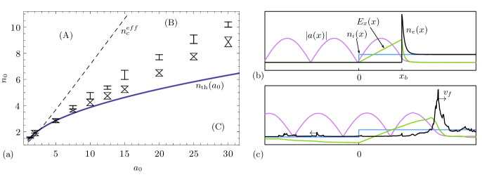
Figure 1: (color online) (a) Effective critical density as a function of the laser field amplitude $a_{0}$ as predicted by the simple relation (2) (dashed, black line). Threshold density $n_{\mathrm{th}}(a_{0})$ below which, according to the cold-fluid theory (cf. Sec. II), no standing wave solutions exist (solid, blue line). RSIT threshold as extracted from our PIC simulations (cf. Sec. IV) with two different pulse rise times: $0.25\tau_{L}$ (error bars) and $4\tau_{L}$ (triangular error bars), where $\tau_{L}=2\pi/\omega_{L}$ is the laser period. (b) Schematic representation of the stationary solution predicted by the cold-fluid theory for the case of total reflection [regions (A) and (B) of panel (a)]. Shown are the electric field $E_{x}(x)$, vector potential of the standing wave $|a(x)|$, and ion (electron) density $n_{i}(x)$ [$n_{e}(x)$], see Sec. II for details. (c) Schematic representation of a typical case of pulse propagation in PIC simulations [for RSIT in region (B) or (C) of panel (a)]. Arrows indicate the direction of electron motion. See Sec. IV for numerical results.

Based on the assumptions stated above, the relativistic cold-fluid model predicts total reflection of the incident pulse, if a certain density threshold $n_{\mathrm{th}}(a_{0})$ is exceeded Cattani et al. (2000); Goloviznin and Schep (2000) [see solid blue line in Fig. 1(a)]. The geometry of the stationary state predicted for $n_{0}>n_{\mathrm{th}}(a_{0})$ is illustrated in Fig. 1(b): the ponderomotive force pushes the electrons deeper into the plasma, creating a charge separation layer (CSL) and an electron density spike [henceforth referred to as compressed electron layer (CEL)] at the edge of the plasma. Electrons in the CEL experience a strong electrostatic field (due to charge separation), which balances the ponderomotive force. The density in the CEL is typically much higher than $n_{c}^{\mathrm{eff}}$ and, thus, pulse propagation is inhibited and a standing wave is formed.

For plasma densities $n_{0}<n_{\mathrm{th}}(a_{0})$, such stationary solutions cease to exist, and one enters the regime of RSIT. particle-in-cell (PIC) simulations Goloviznin and Schep (2000); Eremin et al. (2010), however, indicate that light propagation in this regime is quite different from the traveling-wave solutions discussed earlier Kaw and Dawson (1970). Although a CEL is initially formed, electrons at its edge escape toward the vacuum, leading to force imbalance and allowing the ponderomotive force to push the CEL deeper into the target. The situation is more reminiscent of hole-boring  Wilks et al. (1993); Schlegel et al. (2009) (albeit with immobile ions) with a penetration front moving deeper into the plasma with a constant velocity $v_{f}$, and a Doppler-shifted reflected wave [Fig. 1(c)] (see also Refs. Lefebvre and Bonnaud (1995); Guérin et al. (1996); Sakagami and Mima (1996); Gibbon (2005)).

In this work we show, through PIC simulations, that in the presence of electron heating, induced by the pulse finite rise time, such a propagation mechanism can be activated even for densities $n_{0}>n_{\mathrm{th}}(a_{0})$; see Fig. 1(a). The crucial role is again played by electrons at the edge of the CEL escaping toward the vacuum. However, it has been recently shown that, in the total reflection regime, electrons at the edge of the CEL cannot be forced to escape into the vacuum by infinitesimal perturbations Eremin et al. (2010). To interpret our results, we are thus led to study the response of electrons at the edge of the CEL to finite perturbations. Studying the dynamics of a test-electron in the stationary fields predicted by the cold-fluid model for the CSL and vacuum, we show that electron escape to the vacuum is controlled by separatrices in the single-electron phase space. Moreover, we demonstrate that the perturbation threshold for unbounded motion (electron escape) predicted by our analytical considerations is comparable to the attainable electron momentum due to heating (in the CEL), observed in our PIC simulations at the threshold for RSIT. Finally, we study the effect of laser pulse rise time on electron heating and on the observed modification of the RSIT threshold.

This paper is organized as follows. In Sec. II we revisit some results of the stationary cold-fluid theory that motivate the present study. In Sec. III we analyze the single-electron phase space (for motion in vacuum and charge separation layer), by determining equilibrium solutions (Sec. III.2), studying their linear stability (Sec. III.3), and determining separatrices of bounded and unbounded motion (Sec. III.4). In Sec. IV we present our PIC simulation results and relate them to the analytical results of Sec. III. Finally, we discuss our findings and present our conclusions in Sec. V.

II Review of relativistic cold-fluid theory for RSIT

Throughout the paper, all quantities are normalized to (so-called) relativistic units. In particular, velocity, time, and distance are normalized to the speed of light $c$, inverse laser frequency $\omega_{L}^{-1}$, and inverse vacuum wave number $k_{L}^{-1}=c/\omega_{L}$, respectively. Electric charges and masses are normalized to $e$ and $m_{e}$, respectively, and densities are normalized to the critical density $n_{c}$. Finally, electric fields are normalized to the Compton field $E_{C}=m_{e}\,c\,\omega_{L}/e$.

II.1 Stationary cold plasma model

In this section, we revisit the one-dimensional stationary model proposed independently by Cattani et al. Cattani et al. (2000) and Goloviznin and Schep Goloviznin and Schep (2000) to describe the reflection of an incident relativistic CP laser pulse by a nominally overdense plasma with constant electron density $n_{0}>1$ and a sharp interface with vacuum. Our presentation follows Ref. Cattani et al. (2000).

We consider an incident CP laser pulse propagating along the ${\bf\hat{x}}$-direction with the vector potential

$${\bf A}_{L}(t,x)=\frac{a_{0}}{\sqrt{2}}\,\left[\cos(t-x)\,{\bf\hat{y}}+\sin(t-x)\,{\bf\hat{z}}\right]\,,$$ (3)

where ${\bf\hat{y}}$ and ${\bf\hat{z}}$ denote the unit vectors forming an orthonormal basis in the plane transverse to the laser propagation direction. The pulse is incident from vacuum ($x<0$) onto a semi-infinite plasma ($x>0$). In this work, as in Refs. Goloviznin and Schep (2000); Cattani et al. (2000), we will neglect ion motion.

As outlined in the Introduction, we will consider stationary solutions expressing the balance of the ponderomotive and electrostatic forces, achieved once a CSL of sufficient thickness $x_{b}$ is created, see Fig. 1(b). Assuming total reflection of the laser pulse by the plasma, the balance of the radiation ($\sim a_{0}^{2}$) and electrostatic pressures [$\sim(n_{0}\,x_{b})^{2}/2$], provides a rough estimate for the thickness of the CSL,

$$x_{b}\simeq\frac{\sqrt{2}\,a_{0}}{n_{0}}\,.$$ (4)

The exact expression for $x_{b}$ and the limits of applicability of Eq. (4) are discussed below; see Eq. (17).

In the following, we will look for stationary solutions with vector potential of the form

$${\bf A}(t,x)=a(x)\left[\cos\left(t+\theta/2\right)\,{\bf\hat{y}}+\sin\left(t+\theta/2\right)\,{\bf\hat{z}}\right],$$ (5)

where $\theta$ accounts for the phase jump of the reflected wave

$${\bf A}_{R}(t,x)=\frac{a_{0}}{\sqrt{2}}\,\left[\cos(t+x+\theta)\,{\bf\hat{y}}+\sin(t+x+\theta)\,{\bf\hat{z}}\right]$$

at $x=x_{b}$ and will be computed below. In what follows, we will refer to the spatial function $a(x)$ as the “vector potential.” Note that, in the absence of plasma, we have $a(x)=\sqrt{2}\,a_{0}\cos\left(x+\theta/2\right)$.

Modeling electrons as a relativistic cold fluid, as in Ref. Cattani et al. (2000), we seek stationary solutions satisfying the system of equations

$$\frac{d\phi}{dx} =\frac{d\gamma}{dx}\,,$$ (6)

$$\frac{d^{2}\phi}{dx^{2}} =n_{e}-n_{0}\,,$$ (7)

$$\frac{d^{2}a}{dx^{2}} =\left(\frac{n_{e}}{\gamma}-1\right)\,a\,.$$ (8)

Here, $\phi(x)$ is the electrostatic potential, $n_{e}(x)$ is the electron density and the Lorentz factor is written as $\gamma(x)=\sqrt{1+a^{2}(x)}$ through conservation of transverse canonical momentum. Equation (6) expresses the balance between the electrostatic and ponderomotive forces inside the plasma. Hence, it holds only for $x\geq x_{b}$. Equation (7) is simply Poisson equation and Eq. (8) is the propagation equation (in the Coulomb gauge) for the field prescribed by Eq. (5).

To solve the system of Eqs. (6)–(8), one considers the CSL and the CEL separately. The electron density $n_{e}(x)$, electrostatic field $E_{x}(x)=-d\phi/dx$ and vector potential $a(x)$ are obtained in each layer. Solutions are then matched at the electron front $x=x_{b}$ to ensure continuity of $a(x)$, of its first derivative $da/dx$ and of $E_{x}(x)$.

II.2 Charge separation layer, $0\leq x\leq x_{b}$

The electrostatic field in the CSL, $0\leq x\leq x_{b}$, is easily found by integrating Poisson Eq. (7) with $n_{e}=0$ (no electrons) and boundary condition $E_{x}(0)=0$ (to match the electrostatic field at the vacuum),

$$E_{x}(x)=-\frac{d\phi}{dx}=n_{0}\,x\,.$$ (9)

Thus, the electrostatic field for $0\leq x\leq x_{b}$ increases linearly, up to its maximum value $E_{b}\equiv E_{x}(x_{b})=n_{0}\,x_{b}$. For total reflection at $x=x_{b}$ we can integrate Eq. (8) once to get

$$\left.\left(\frac{da}{dx}\right)^{2}\right|_{x=x_{b}}=2\,a_{0}^{2}-a_{b}^{2}\,,$$ (10)

where $a_{b}=a(x_{b})$ is the vector potential at the plasma boundary. Here, we write the amplitude of the standing wave arising from the combination of the incident and reflected waves $A_{L}$ and $A_{R}$, respectively, as

$$a(x)=\sqrt{2}\,a_{0}\,\sin\left[\arcsin\left(\frac{a_{b}}{\sqrt{2}\,a_{0}}\right)-(x-x_{b})\right]\,,$$ (11)

which implies that in Eq. (5) we have $\theta/2=\pi/2-\arcsin(a_{b}/\sqrt{2}\,a_{0})-x_{b}$. At this point, there are two unknown quantities, $x_{b}$ and $a_{b}$, which will be determined self-consistently by considering the region $x\geq x_{b}$. Note that we assume $a_{b}>0$, while from Eq. (11) we have $a^{\prime}(x_{b})<0$ so that the ponderomotive force $d\gamma/d\,x=\gamma^{-1}\,a\,da/dx$ pushes electrons deeper into the plasma, thus balancing the electrostatic force.

II.3 Compressed electron layer, $x\geq x_{b}$

We now derive equations for the electron density, vector potential and electrostatic field in the plasma, $x\geq x_{b}$. Combining Eqs. (6) and (7), one can rewrite the normalized electron density in the plasma as a function of the vector potential $a(x)$ and its first two derivatives,

$$n_{e}(x)=n_{0}+\frac{1}{\sqrt{1+a^{2}}}\,\left[a\,\frac{d^{2}a}{dx^{2}}+\frac{1}{1+a^{2}}\,\left(\frac{da}{dx}\right)^{2}\right].$$ (12)

Substituting Eq. (12) in Eq. (8), we obtain a differential equation for the vector potential only:

$$\frac{d^{2}a}{dx^{2}}=\frac{a}{1+a^{2}}\!\left(\frac{da}{dx}\right)^{2}\!-\!\left(1\!+\!a^{2}\!-\!n_{0}\sqrt{1+a^{2}}\right)\!a\,.$$ (13)

In the case of total reflection, Eq. (13) describes the evanescent field in the overdense plasma, and has to be solved with boundary conditions $a(x)\rightarrow 0$ and $da/dx\rightarrow 0$ for $x\rightarrow+\infty$ . Equation (13) admits a first integral,

$$\frac{1}{2(1+a^{2})}\left(\frac{d\,a}{d\,x}\right)^{2}-\frac{1}{2}\left(2n_{0}\sqrt{1+a^{2}}-a^{2}\right)=-n_{0},$$ (14)

which may be used to derive a solution that satisfies the required boundary conditions Marburger and Tooper (1975),

$$a(x)=\frac{2\sqrt{n_{0}\,(n_{0}-1)}\,\cosh\left[(x-x_{0})/\lambda_{s}\right]}{n_{0}\,\cosh^{2}\left[(x-x_{0})/\lambda_{s}\right]-(n_{0}-1)}\,,$$ (15)

where $\lambda_{s}=(n_{0}-1)^{-1/2}$ is the classical skin-depth, and $x_{0}$ is determined by ensuring the continuity of the vector potential at $x=x_{b}$.

With $a(x)$ inside the plasma provided by Eq. (15), one obtains $n_{e}(x)$ from Eq. (12), while Eq. (6) provides the electrostatic field in this region,

$$E_{x}(x)=-\frac{d}{dx}\sqrt{1+a^{2}}\,.$$ (16)

Equation (16) together with Eqs. (9) and (10) and the continuity of the electrostatic field at $x=x_{b}$ gives an explicit expression for the position of the electron front,

$$x_{b}=\frac{a_{b}}{n_{0}}\,\sqrt{\frac{2\,a_{0}^{2}-a_{b}^{2}}{1+a_{b}^{2}}}\,.$$ (17)

Finally, from Eqs. (10) and (14), one obtains:

$$\frac{2\,a_{0}^{2}+a_{b}^{4}}{1+a_{b}^{2}}=2\,n_{0}\,\left(\sqrt{1+a_{b}^{2}}-1\right)\,.$$ (18)

This equation defines, for a given incident laser field amplitude $a_{0}$ and initial plasma density $n_{0}$, the maximum evanescent field $a_{b}$ in the plasma. Solutions $a_{b}$ of Eq. (18) should satisfy the additional condition

$$2\,a_{0}^{2}-a_{b}^{2}\geq 0\,,$$ (19)

which follows from Eq. (10).

Note that, in the limit $1\ll a_{b}\ll a_{0}$, Eq. (17) allows us to recover the approximate result Eq. (4). On the other hand, from Eqs. (17)–(18) we find that in the limit $a_{b}\ll 1$ (correspondingly $a_{0}^{2}\ll n_{0}$) $x_{b}\simeq 2\,a_{0}^{2}/n_{0}^{3/2}$.

II.4 Threshold for RSIT

For a given plasma density $n_{0}$, Eq. (18) admits a solution only when the maximum evanescent field $a_{b}$ satisfies Cattani et al. (2000)

$$2\,(n_{0}+a_{b}^{2})\leq 3\,n_{0}\,\sqrt{1+a_{b}^{2}}\,.$$ (20)

As shown in Ref. Goloviznin and Schep (2000), for $n_{0}<3/2$, solutions compatible with Eq. (19) can only be found in the region $a_{0}^{2}\leq 2\,n_{0}(n_{0}-1)$. Thus, in this case, the threshold incident laser amplitude reads

$$a_{\mathrm{th}}^{2}=2\,n_{0}(n_{0}-1)\,.$$ (21)

For $n_{0}>3/2$ condition (19) is always fulfilled and Eq. (20) defines the regime of total reflection. The threshold for RSIT corresponds to equality in Eq. (20). The maximum evanescent field at the threshold then reads

$$a_{B}^{2}=n_{0}\,\left(\frac{9}{8}\,n_{0}-1+\frac{3}{2}\,\sqrt{\frac{9}{16}\,n_{0}^{2}-n_{0}+1}\right)\,.$$ (22)

The threshold incident laser field amplitude $a_{th}$ above which RSIT occurs in a plasma with initial density $n_{0}$ is obtained by substituting $a_{b}=a_{B}$ from Eq. (22) in Eq. (18),

$$a_{\mathrm{th}}^{2}=n_{0}\,(1+a_{B}^{2})\,\left(\sqrt{1+a_{B}^{2}}-1\right)-a_{B}^{4}/2\,.$$ (23)

Depending on the density range, Eq. (21), respectively Eqs. (22)–(23), define a threshold amplitude $a_{\mathrm{th}}(n_{0})$, above which RSIT occurs, for a given plasma density. Alternatively, for a given incident amplitude $a_{0}$, we may read Eq. (21), respectively Eqs. (22)–(23), as defining an effective critical density $n_{\mathrm{th}}(a_{0})$ below which RSIT occurs. This is illustrated in Fig. 1(a). Equation (21) yields

$$n_{\mathrm{th}}(a_{0})=\frac{1}{2}\left(1+\sqrt{1+2a_{0}^{2}}\right)\,,\quad n_{\mathrm{th}}<3/2\,,$$ (24)

while Eqs. (22)–(23) can be inverted analytically in the limit $n_{0}\gg 1$, yielding

$$n_{\mathrm{th}}(a_{0})\simeq\frac{2}{9}\left(3+\sqrt{9\sqrt{6}\,a_{0}-12}\,\right)\,,\quad n_{\mathrm{th}}\gg 1\,.$$ (25)

Thus, the asymptotic behavior of $n_{\mathrm{th}}(a_{0})$ in the limit $a_{0}\gg 1$ is $n_{\mathrm{th}}\propto a_{0}^{1/2}$, a much more restricting condition than Eq. (2), which for large $a_{0}$ becomes $n_{c}^{\mathrm{eff}}\propto a_{0}$.

As discussed in the Introduction, our PIC simulations indicate that for pulses with finite rise time, the transition between total reflection and RSIT occurs within the limits set by Eqs. (25) and (2) and, moreover, depends on the pulse rise time. In order to explain this discrepancy, we will now study single electron dynamics in the stationary fields (in vacuum and CSL) calculated above.

III Single electron dynamics

III.1 Equations of single electron motion

The equations of motion for an electron in the region $x\leq x_{b}$ (i.e. in the vacuum and CSL), in the case of total reflection, read

$$\dot{x} =p_{x}/\gamma\,,$$ (26)

$$\dot{p}_{x} =-\frac{\partial\,\gamma}{\partial\,x}-E_{x}(x)\,,$$ (27)

where we have used conservation of transverse canonical momentum to write the electron $\gamma$ factor as

$$\gamma(x,p_{x})=\sqrt{1+a^{2}(x)+p_{x}^{2}},$$ (28)

$p_{x}$ is the electron’s longitudinal momentum, the electrostatic field $E_{x}(x)$ and vector potential $a(x)$ are given by Eqs. (9) and (11), respectively, and dotted quantities are differentiated with respect to time.

Equations (26)–(27) can be derived from the Hamiltonian:

$$H(x,p_{x})=\gamma(x,p_{x})-\phi(x)\,,$$ (29)

where the electrostatic potential reads

$$\phi(x)=\begin{cases}0\,,&x<0\,,\\ -\frac{1}{2}n_{0}\,x^{2},&0\leq x\leq x_{b}\,.\end{cases}$$ (30)

The Hamiltonian $H(x,p_{x})$ is a conserved quantity and we can thus write an explicit expression for the electron orbit with initial conditions $x_{0},p_{x}{}_{0}$:

$$p_{x}(x)=\pm\,\sqrt{\left[H(x_{0},p_{x}{}_{0})+\phi(x)\right]^{2}-a^{2}(x)-1}\,.$$ (31)

Equation (31) suffices to plot portraits of the single-electron phase space, as shown in Fig. 2. In the following subsections we explain how the several solutions depicted in Fig. 2 are interrelated, in order to understand how phase space geometry affects the threshold of RSIT.

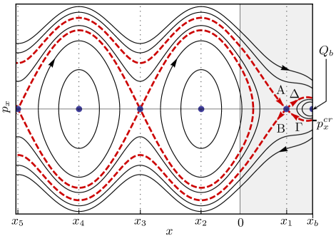
Figure 2: (color online) Typical single-electron phase space portrait for Eqs. (26)–(27). The first six equilibria $\mathrm{Q}_{b},\,\mathrm{Q}_{1},\,\ldots,\,\mathrm{Q}_{5}$ corresponding to positions $x_{b},\,x_{1},\,\ldots,\,x_{5}$ and zero momentum are shown as blue dots. Separatrices are shown as red, dashed lines and some typical trajectories are depicted as black, solid lines. The CSL is depicted as a gray-shaded area.

III.2 Equilibrium solutions

The simplest type of solutions of Eqs. (26)–(27) are equilibrium solutions for which $\dot{x}=\dot{p}_{x}=0$. We have already seen that, within the framework of the stationary cold-fluid model, the force balance Eq. (6) is satisfied in the plasma and in particular at $x=x_{b}$. Thus, the point $(x,p_{x})=(x_{b},0)$ is an equilibrium which we label as $\mathrm{Q}_{b}$. (For the same reasons, any point in the plasma with $p_{x}=0$ will be an equilibrium.)

In the CSL and vacuum, on the other hand, the ponderomotive and electrostatic forces are not balanced in general, and equilibria for the motion of a test particle have to be found by setting $\dot{x}=\dot{p}_{x}=0$ in Eqs. (26)–(27). We label equilibria at the left of $\mathrm{Q}_{b}$ as $\mathrm{Q}_{m}$, $m=1,\,2,\dots$, where $m$ increases with decreasing $x_{m}$.

For $x<0$ (in the vacuum) equilibria correspond to $\partial_{x}\gamma=\frac{a}{\gamma}\frac{da}{dx}=0$, i.e. $a=0$ or $da/dx=0$, which, according to Eq. (11), leads to

$$x_{k}^{-}=\arcsin\left(\frac{a_{b}}{\sqrt{2}\,a_{0}}\right)+x_{b}-k\pi/2\,.$$ (32)

Here, $k$ can be any positive integer provided that $x_{k}^{-}<0$, and $k$ even or odd correspond to $a(x_{k}^{-})=0$ or $a^{\prime}(x_{k}^{-})=0$, respectively. We note that in our labeling scheme, index $k$ in $x_{k}^{-}$ does not always correspond to index $m$ in labeling of equilibria $\mathrm{Q}_{m}$, i.e. we will generally have $x_{m}=x_{k}^{-}$ with $m\neq k$. 

For $0\leq x\leq x_{b}$ (in the CSL), the equilibrium condition $\partial_{x}\phi=\partial_{x}\gamma$ must be solved numerically, using Eqs. (11) and (30) for $a(x)$ and $\phi(x)$, respectively. A perturbative solution can be obtained in the neighborhood of $x_{b}$, by expanding $\dot{p}=-\frac{\partial\,\gamma}{\partial\,x}-E_{x}(x)=0$ to second order in $x-x_{b}$. We obtain two solutions, $x=x_{b}$ and

$$x_{1}\simeq x_{b}+\frac{2(1+a_{b}^{2})^{2}[2(a_{b}^{2}+n_{0})-3\,n_{0}(1+a_{b}^{2})^{1/2}]}{a_{b}(2a_{0}^{2}-a_{b}^{2})^{1/2}(4+2a_{b}^{2}+a_{b}^{4}+6a_{0}^{2})}\,.$$ (33)

Comparing Eq. (33) with condition (20), we see that $x_{1}\leq x_{b}$, as long as a standing wave solution exists, i.e. for $n_{0}\geq n_{\mathrm{th}}$. At threshold, $n_{0}=n_{\mathrm{th}}$, we have $x_{1}=x_{b}$. That is, if we approach the RSIT threshold (as predicted by cold-fluid theory), the equilibrium $\mathrm{Q}_{1}$ approaches $\mathrm{Q}_{b}$ until the two states coalesce, see Fig. 3(c).

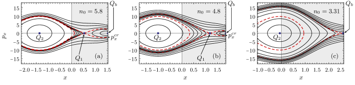
Figure 3: (color online) For a given laser field amplitude, here $a_{0}=7$, the absolute value of the critical momentum for an electron to escape to the vacuum $|p_{x}^{\mathrm{cr}}|$ decreases as $n_{0}$ decreases. Shown are the cases (a) $n_{0}=5.8$, (b) $n_{0}=4.8$, (c) $n_{0}=3.31$. Color-code is the same as described in the caption of Fig. 2. In panel (c) equilibria $\mathrm{Q}_{1}$ and $\mathrm{Q}_{b}$ cannot be distinguished within the resolution of this plot, $n_{0}$ being slightly above the cold-fluid theory threshold $n_{\mathrm{th}}=3.30458$. Note that the scale of $x$ and $p_{x}$ has been kept the same in all panels.

III.3 Stability of equilibria

Linear stability analysis of the equilibria determined in Sec. III.2 can give us information on the behavior of orbits in the neighborhood of the equilibria. For notational convenience, we define phase space variables $\zeta=(\zeta_{1},\zeta_{2})\equiv(x,\,p_{x})$ and rewrite the equations of motion [Eq. (26) and Eq. (27)] in the form

$$\dot{\zeta}_{i}=F_{i}(\zeta)\,.$$ (34)

where $F_{1}(\zeta)=\zeta_{2}/\gamma$ and $F_{2}(\zeta)=-\frac{\partial\,\gamma}{\partial\,\zeta_{1}}-E_{x}(\zeta_{1})$. Considering infinitesimal perturbations in the neighborhood of equilibrium $\zeta^{(m)}$, and substituting $\zeta(t)=\zeta^{(m)}+\xi(t)$, with $\lVert\xi\rVert\ll 1$, in Eq. (34), one obtains

$$\dot{\xi}=\mathcal{A}(\zeta_{m})\xi\,,$$ (35)

where the Jacobian matrix $\mathcal{A}(\zeta_{m})$, with elements

$$A_{ij}=\left.\frac{\partial F_{i}}{\partial\zeta_{j}}\right|_{\mathrm{Q}_{m}}\,,$$ (36)

has been introduced.

Solutions of the linear system Eq. (35) are of the form $\xi(t)=\exp[\mathcal{A}(\zeta_{m})t]\xi(0)$, and thus the linear stability of equilibrium $\mathrm{Q}_{m}$ is determined by the eigenvalues of the Jacobian matrix. In Hamiltonian systems with one degree of freedom, classification of equilibria $\mathrm{Q}_{m}$ by linear stability is straightforward (see, e.g., Ref. Lichtenberg and Lieberman (1992)), as there are only two possibilities:

• $\mathcal{A}(\zeta_{m})$ has a pair of real eigenvalues $\lambda_{1}=-\lambda_{2}>0$. Solutions then deviate from $\mathrm{Q}_{m}$ at an exponential rate, $\lVert\xi(t)\rVert\sim e^{\lambda_{1}t}\lVert\xi(0)\rVert$, and the equilibrium (called a saddle) is unstable.

• $\mathcal{A}(\zeta_{m})$ has a conjugate pair of purely imaginary eigenvalues $\lambda_{1}=\lambda_{2}^{*}=iw$. Solutions then oscillate around $\mathrm{Q}_{m}$ with period $2\pi/w$, and the equilibrium (called a center) is (neutrally) stable.

Taking into account equilibrium conditions $\dot{x}=\dot{p}_{x}=0$, we find from Eq. (36)

$$\mathcal{A}(\zeta_{m})=\left(\begin{array}[]{cc}0&1/\gamma_{m}\\ A_{21}&0\end{array}\right),$$

where

$$A_{21}=\frac{1}{\gamma}\left[\frac{a^{2}_{m}\,(a^{\prime}_{m})^{2}}{\gamma^{2}_{m}}-(a^{\prime}_{m})^{2}+a^{2}_{m}\right]-\begin{cases}n_{0}\,,&x>0\,,\\ 0\,,&x<0\,.\end{cases}$$

Here, we have defined $a_{m}=a(x_{m})$, $a^{\prime}_{m}=a^{\prime}(x_{m})$, $\gamma_{m}=\sqrt{1+a^{2}(x_{m})}$, and we have used Eq. (8).

Eigenvalues of $\mathcal{A}(\zeta_{m})$ are given by

$$\lambda_{1,2}(x_{m})=\pm\sqrt{A_{21}/\gamma_{m}}\,.$$ (37)

In the vacuum, $x<0$, equilibria correspond to either $a(x_{k}^{-})=0$ ($k$ even, nodes of the standing wave) or $a^{\prime}(x_{k}^{-})=0$ ($k$ odd, antinodes of the standing wave), where the $x_{k}^{-}$ are given by Eq. (32). Then, Eq. (37) yields by using Eqs. (32) and (11),

$$\lambda_{1,2}(x_{k}^{-})=\pm\begin{cases}i\sqrt{2}\,a_{0}\,,&k\text{ even,}\\ \frac{\sqrt{2}\,a_{0}}{\sqrt{1+2\,a_{0}^{2}}}\,,&k\text{ odd.}\end{cases}$$ (38)

Thus, in the vacuum, equilibria alternate between being (neutrally) stable ($k$ even, nodes) and unstable ($k$ odd, antinodes).

In the CSL, $x>0$, we have

$$\lambda_{1,2}(x_{m})=\pm\frac{1}{\gamma_{m}^{2}}\sqrt{\gamma_{m}^{2}(a_{m}^{2}-(a^{\prime}_{m})^{2})+a_{m}^{2}(a^{\prime}_{m})^{2}-\gamma_{m}^{3}n_{0}}\,.$$

For the equilibrium $\mathrm{Q}_{b}$ at the plasma boundary, $x=x_{b}$, we get from Eq. (11)

$$\lambda_{1,2}(x_{b})=\pm\sqrt{a_{b}^{4}+2a_{b}^{2}-2a_{0}^{2}-n_{0}(1+a_{b}^{2})^{3/2}}/(1+a_{b}^{2})\,.$$ (39)

Linear (neutral) stability of $\mathrm{Q}_{b}$ requires

$$a_{b}^{4}+2a_{b}^{2}-2a_{0}^{2}-n_{0}(1+a_{b}^{2})^{3/2}<0\,,$$

or, using Eq. (18) to eliminate $a_{0}$,

$$2(a_{b}^{2}+n_{0})-3n_{0}(1+a_{b}^{2})^{1/2}<0\,.$$ (40)

The same condition for linear stability of the equilibrium at $x_{b}$ was obtained by Eremin et al.  Eremin et al. (2010) by considering the infinitesimal variation in electrostatic and ponderomotive force experienced by an electron whose position has been perturbed infinitesimally to $x_{b}-|\delta x|$. Condition (40) also coincides with condition (20) of existence of a stationary standing wave obtained by Cattani et al. Cattani et al. (2000). Therefore, as long as an equilibrium at $x_{b}$ exists, it is neutrally stable.

Assessing stability of the equilibria with $0<x_{1}<x_{b}$ analytically is somewhat more difficult [even when an explicit expression such as Eq. (33) is available]. We can, however, conclude that $\mathrm{Q}_{1}$ is an unstable equilibrium on topological grounds. If we assume $\mathrm{Q}_{1}$ to be stable, then motion in its neighborhood would be oscillatory. Therefore, a point $(x_{s},0)$ in phase space with $x_{1}<x_{s}<x_{b}$ would be shared by oscillatory solutions encircling $\mathrm{Q}_{1}$ and $\mathrm{Q}_{b}$ (in phase space). This would contradict uniqueness of solutions, unless the point $(x_{s},0)$ were to be reached in infinite time, i.e. unless it is an unstable equilibrium. However, by construction there is no equilibrium beween $Q_{1}$ and $Q_{b}$. In fact, the degenerate oscillations introduced in this argument, which reach $Q_{1}$ in infinite time, are the familiar separatrices of bounded and unbounded motion, which we will now study in detail.

III.4 Separatrices

In the vacuum ($x<0$), all unstable equilibria at $x_{k}^{-}$ (with $k$ odd) correspond to the same value of $H$,

$$H(x_{k}^{-},0)=\sqrt{1+2\,a_{0}^{2}}\,.$$ (41)

Conservation of $H$, thus allows for a heteroclinic connection, i.e., for an orbit which starts infinitesimally close to $\mathrm{Q}_{k}$ and ends infinitesimally close to $\mathrm{Q}_{k+2}$ or $\mathrm{Q}_{k-2}$ (in infinite time). According to Eq. (31) these orbits obey

$$p_{x}(x)=\pm\sqrt{2a_{0}^{2}-a^{2}(x)}\,.$$ (42)

Heteroclinic connections, Eq. (42), act as separatrices of bounded and unbounded motion, see Fig. 2.

Within the CSL ($0<x<x_{b}$), an unstable equilibrium, e.g.  $\mathrm{Q}_{1}$ in Fig. 2, will in general have $H(x_{1},0)\neq H(x_{3},0)$ since $H$ now also includes an electrostatic field contribution. Therefore, a heteroclinic connection from $\mathrm{Q}_{3}$ to $\mathrm{Q}_{1}$ is not possible, and the separatrix starting out at $\mathrm{Q}_{3}$ is a homoclinic connection, i.e. an orbit that returns to $\mathrm{Q}_{3}$ in infinite time. For the same reason, the separatrix labeled $\mathrm{B}$ in Fig. 2 starts in the neighborhood of $\mathrm{Q}_{1}$ and wanders off to $x=-\infty$, while the separatrix labeled $\mathrm{A}$ starts at $x=-\infty$ and ends at $\mathrm{Q}_{1}$.

Of greatest importance in the following discussion are the separatrices labeled $\Gamma$ and $\Delta$, as they determine the region within which motion close to $\mathrm{Q}_{b}$ is oscillatory. The equations of the separatrices $\Gamma$ and $\Delta$ are given by Eq. (31) with $(x_{0},p_{x}{}_{0})=(x_{1},0)$ [on separatrix $\Gamma$, motion is backwards in time and $(x_{1},0)$ is a final, rather than initial, condition]. The point on separatrix $\Gamma$ at position $x_{b}$ (at the plasma boundary) then defines a critical momentum $p_{x}^{\mathrm{cr}}$, given by

$$p_{x}^{\mathrm{cr}}=-\left[\left[\sqrt{1+a^{2}(x_{1})}+n_{0}(x_{1}^{2}-x_{b}^{2})/2\right]^{2}-a_{b}^{2}-1\right]^{1/2}\,.$$ (43)

If a single electron at the edge of the plasma $x_{b}$ is given an initial momentum $-|\Delta p_{x}|$, with $|\Delta p_{x}|<|p_{x}^{\mathrm{cr}}|$, it will move within the limits set by separatrices $\Gamma$ and $\Delta$, returning back to the plasma. If, on the other hand $|\Delta p_{x}|>|p_{x}^{\mathrm{cr}}|$, the electron’s motion will be unbounded and it will escape to the vacuum. Alternatively, one can define a critical value of the Hamiltonian

$$H^{\mathrm{cr}}\equiv H(x_{1},0)=\sqrt{1+a^{2}(x_{1})}+n_{0}\,x_{1}^{2}/2\,.$$ (44)

Motion of electrons with $H(x_{b},p_{x})>H^{\mathrm{cr}}$ and $p_{x}<0$ will be unbounded.

Equation (43) shows that $|p_{x}^{\mathrm{cr}}|$ is always non-zero as long as $x_{1}\neq x_{b}$; for fixed $a_{0}$ it becomes smaller as $n_{0}$ decreases and $x_{1}$ approaches $x_{b}$, vanishing at the threshold $n_{\mathrm{th}}$ given by Eq. (20). This behavior is illustrated in Fig. 3 for $a_{0}=7$. (See also Fig. 10.)

With the above results it becomes clear that finite perturbations of initial conditions of electrons at the edge of the plasma, for example due to longitudinal electron heating, could lead to electrons escaping toward the vacuum even when $\mathrm{Q}_{b}$ is stable in the linear approximation, provided that the perturbation (here negative momentum) is large enough. Our main conclusion is that pulse propagation by expulsion of electrons toward the vacuum could occur for densities higher than the threshold density $n_{\mathrm{th}}$ predicted by the cold fluid approximation. In Sec. IV we show that electron heating at the edge of the plasma indeed provides a mechanism by which electrons acquire sufficient momentum to escape toward the vacuum.

IV PIC simulations

To investigate the transition from total reflection to RSIT, we perform PIC simulations Birdsall and Langdon (1991) using the one-dimensional in space, three-dimensional in velocity (1D3V) code Squash Grech et al. (2012). The code uses the finite-difference, time-domain approach for solving Maxwell’s equations Taflove and Hagness (2005), and the standard (Boris) leap-frog scheme for solving the macro-particle equations of motion Boris (1970). Charge conservation is ensured by using the method proposed by Esirkepov when projecting the currents Esirkepov (2001).

In all simulations presented here, ions are immobile and only electron motion is considered. We use the spatial resolution $dx=\lambda_{L}/500$ and time step $dt=\tau_{L}/1000$, where $\lambda_{L}$ and $\tau_{L}$ are the laser wavelength and duration of one optical cycle, respectively. Up to 1000 macro-particles per cell have been used.

The plasma extends from $x=0$ to $x=L_{p}$, with a constant initial density $n_{0}$ and electron temperature $T_{0}\simeq 5\cdot 10^{-4}$ (in units of $m_{e}c^{2}$). The plasma size $L_{p}$ is chosen so that $L_{p}>c\,\tau_{\mathrm{int}}$, where $\tau_{\mathrm{int}}$ is the laser-plasma interaction time. Hence, the plasma is long enough to be considered semi-infinite. The CP laser pulse [as described by Eq. (3)] is incident from $x<0$ onto the plasma. In this work we consider laser field amplitudes in the range $a_{0}=1-30$. The laser pulse profile is trapezoidal, i.e. the intensity increases linearly within a rise time $\tau_{r}$, up to a maximum value $a_{0}^{2}/2$, and we consider the exemplary cases $\tau_{r}=0.25\,\tau_{L}$ and $\tau_{r}=4\,\tau_{L}$.

Figure 1(a) summarizes our findings on RSIT, comparing the threshold density $n_{\mathrm{th}}(a_{0})$ predicted by Cattani et al. Cattani et al. (2000) with our 1D3V PIC simulation results. In order to determine whether RSIT occurs or not in a simulation, the position $x_{b}$ of the maximum electrostatic field is plotted as a function of time (see Fig. 4). The regime of total reflection is characterized by the formation of a CSL with (approximately) constant thickness $x_{b}$ (Fig. 4, $n_{0}=6.7-8$). On the other hand, RSIT is associated with front propagation at an approximately constant velocity $v_{f}$, so that the position of the maximum electrostatic field increases linearly with time (Fig. 4, $n_{0}=5.75-6$). This allows us to place lower and upper bounds on RSIT threshold density, for a certain $a_{0}$, indicated by error bars in Fig. 1. For densities within these limits, it is hard to decide whether RSIT occurs or not (Fig. 4, $n_{0}=6.25$).

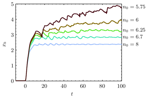
Figure 4: (color online) Position of the maximum value of the electrostatic field $x_{b}$ as a function of time from PIC simulations with different densities and $a_{0}=15$, $\tau_{r}=0.25\,\tau_{L}$.

In the next subsections we examine in detail typical cases of total reflection and front penetration.

IV.1 Total reflection

Whenever total reflection occurs, the system eventually settles to a quasi-stationary state. The size of the charge separation layer $x_{b}$ remains constant or slightly oscillatory around a value that is found to be in good agreement with the theoretical prediction of the cold-fluid model [Eq. (17)], see Fig. 5. The same is true for the field and density profiles; a worst case agreement is shown in Fig. 6, where the quasistationary state reached for $a_{0}=15$, $n_{0}=7$ and $\tau_{r}=0.25\tau_{L}$ is close to the numerical RSIT threshold (the agreement becomes better for higher $n_{0}$ or larger $\tau_{r}$). Although the density profile presents oscillations, the fields in the CSL and vacuum agree very well with the predictions of cold-fluid theory. This justifies a posteriory our use of stationary cold fluid theory predictions for the fields in the vacuum to analyze single electron phase space in Sec. III. The phase portrait for $a_{0}=15$, $n_{0}=7$ and $\tau_{r}=0.25\tau_{L}$ is shown in the top row of Fig. 7. It is clearly seen that electrons in the CEL do not have zero longitudinal momentum $p_{x}$ as the stationary cold-fluid model suggests, but rather oscillate around $x_{b}$ [the latter being in good agreement with Eq. (17)]. As the minimum momentum attained by electrons, which we will call $p_{x}^{\mathrm{min}}$, is smaller in absolute value than the critical momentum required to move beyond the limits set by the separatrices of bounded and unbounded motion, $|p_{x}^{\mathrm{min}}|<|p_{x}^{\mathrm{cr}}|$, electrons which cross the plasma boundary $x_{b}$ do not escape into the vacuum but rather re-enter the CEL.

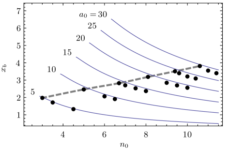
Figure 5: (color online) Comparison of cold-fluid model prediction for $x_{b}$ (blue, solid lines) with the (time-averaged) position of the maximum electrostatic field in our PIC simulations (dots), with $\tau_{r}=0.25\,\tau_{L}$. For values of $n_{0}$ to the left of the thick, gray, dashed line RSIT occurs and $x_{b}$ does not reach a constant average value in our PIC simulations.

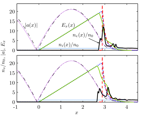
Figure 6: (color online) Electron density and field profiles from PIC simulations for $a_{0}=15$, $n_{0}=7$ at $t=2.55\,\tau_{L}$ (top panel) and $t=2.95\,\tau_{L}$ (bottom panel). The stationary cold-fluid model solution for the electron density (red, dashed line), electrostatic field (blue, dotted line) and vector potential envelope (black, dash-dotted line) are also shown. Note that densities have been rescaled to the unperturbed density $n_{0}$ for better readability.

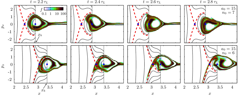
Figure 7: (color online) Comparison between phase space separatrices as predicted by the stationary, cold-fluid model, and single particle distribution function $f(x,p_{x})$ from PIC simulation results for $a_{0}=15$ and $n_{0}=7$ (top row), $n_{0}=6$ (bottom row) and rise time $\tau_{r}=0.25\,\tau_{L}$. Snapshots are shown $0.2\,\tau_{L}$ apart. The plasma boundary ($x=x_{b}$), as predicted by the cold-fluid model, is indicated by a black, dotted, vertical line. The color coding of trajectories follows Fig. 2. Note the logarithmic scale in the color coding of $f(x,p_{x})$.

As can be seen in Fig. 4, for $n_{0}=6.7-8$, the position of the plasma boundary $x_{b}$ oscillates in time, leading to oscillations of the maximum electrostatic field. These oscillations can be related to the excursion of electrons in the region $x<x_{b}$, cf.  the top panel of Figure 7. To verify this, we plot in Fig. 8 the period $T_{\mathrm{osc}}$ of these oscillations for different $a_{0}$ and $n_{0}$ well in the regime of total reflection. The frequency of these oscillations is not linked to the plasma frequency (observe the dependence on $a_{0}$ in Fig. 8) but rather on the frequency of oscillations of electrons around the equilibrium $Q_{b}$. If we ignore the role of the self-consistent fields within the plasma, the characteristic period of oscillation in the linear neighborhood of $Q_{b}$ reads $T_{Q_{b}}=2\pi/\operatorname{Im}\lambda_{1}$, where $\lambda_{1}$ is the eigenvalue given by Eq. (39). As shown in Fig. 8, we find $T_{\mathrm{osc}}\propto T_{Q_{b}}$. We also note the similarity of these oscillations with the so-called piston oscillations in laser hole-boring Schlegel et al. (2009), although in the present case the oscillations only involve electrons.

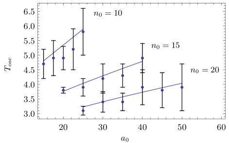
Figure 8: (color online) Period of oscillations of $x_{b}$ as a function of $a_{0}$ for three different $n_{0}$. Points with error bars correspond to the periods as deduced from our PIC simulations, while the solid lines correspond to $T_{\mathrm{osc}}=1.75\,T_{Q_{b}}=1.75\times 2\pi/\operatorname{Im}\lambda_{1}$, where $\lambda_{1}$ is given by Eq. (39).

IV.2 RSIT

The cold fluid model presented in Sec. II predicts a sharp threshold, either for density $n_{0}$ or laser amplitude $a_{0}$, for RSIT. However, as already mentioned above, one of the main results of this paper is that our PIC simulations clearly show RSIT in a parameter region where the cold fluid model predicts total reflection [area (B) in Fig. 1(a)]. A typical case of RSIT in this regime is presented in Fig. 9, where $a_{0}=15$, $n_{0}=5.5$ and $\tau_{r}=0.25\tau_{L}$. Charge separation and compressed electron layers are formed in the early stages of interaction, with profiles that agree well with the predictions of cold-fluid theory. However, electrons escape the CEL, and the pulse can propagate (see middle row of Fig. 9). The mechanism of propagation is rather complex, but its initial phase can be intuitively understood as follows. When a sufficiently high number of electrons escapes from the CEL to the vacuum, the electrostatic field within the CSL decreases, the ponderomotive force is no longer balanced and the laser pulse can push the CEL deeper into the plasma. The increase of the CSL size tends to compensate the force imbalance, but as more and more electrons escape, the pulse continues to propagate deeper into the plasma. We note that once electrons escape and propagation commences the stationary model is no longer valid and electron dynamics becomes complex, with electron bunches leaving and re-entering the plasma (see Fig. 9 and Ref. Eremin et al. (2010)).

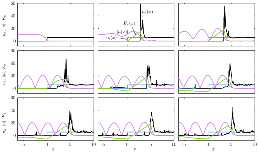
Figure 9: (color online) Field and density evolution for RSIT above the cold-fluid theory threshold, $a_{0}=15$, $n_{0}=5.5$. Snapshots are taken one laser period apart, starting at $t=0$.

To understand how the shrinking of the width of separatrices in phase space with decreasing density (and constant $a_{0}$) leads to propagation, we examine the phase space portrait for $a_{0}=15$, $n_{0}=6.0$ and $\tau_{r}=0.25\,\tau_{L}$, which corresponds to a case just below the numerical density threshold for RSIT, see the bottom row of Fig. 7. In this case, the minimum momentum acquired by electrons in the CEL satisfies $|p_{x}^{\mathrm{min}}|>|p_{x}^{\mathrm{cr}}|$ and electrons move outside the separatrix of bounded and unbounded motion, eventually reaching the vacuum, while the CEL moves deeper into the plasma.

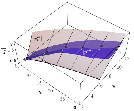
Figure 10: (color online) The absolute value of momentum $|p_{x}^{\mathrm{cr}}|$ corresponding to the separatrix of bounded and unbounded motion for electrons at $x_{b}$ for different $a_{0}$ and $n_{0}$, according to Eq. (43) is shown as a light-gray surface. An estimate of the absolute value of the minimum momentum $|p_{x}^{\mathrm{min}}|$ attained by electrons in the CEL, as determined by our PIC simulations with $\tau_{r}=0.25\tau_{L}$, is shown as a dark-blue surface. The light- and dark-colored points represent PIC simulation results corresponding to onset of RSIT and total reflection, respectively, for $a_{0}=5,\,10,\ldots,30$. On both surfaces, lines of constant $a_{0}$ are drawn to guide the eye. The contour $|p_{x}^{\mathrm{cr}}|=0$ (black, thick, solid line) corresponds to the threshold for RSIT predicted by cold-fluid theory.

Figure 10 provides a further verification of the role the longitudinal electron heating plays in enabling electrons to escape from the CEL into the vacuum. We use Eq. (43) to plot $|p_{x}^{\mathrm{cr}}|$ as a function of $a_{0}$ and $n_{0}$ (light-gray surface). For a given rise time, here $\tau_{r}=0.25\,\tau_{L}$, we also plot, as a function of $a_{0}$ and $n_{0}$, the absolute value of the minimum momentum $|p_{x}^{\mathrm{min}}|$ acquired by electrons in the CEL as inferred from our PIC simulations (dark-blue surface). To reduce noise we average $|p_{x}^{\mathrm{min}}|$ over one laser period (starting at $t\simeq 2\tau_{L}$), or at most until electrons escape. Thus, our $|p_{x}^{\mathrm{min}}|$ is generally slightly underestimated, however the intersection of the two surfaces $|p_{x}^{\mathrm{cr}}|$ and $|p_{x}^{\mathrm{min}}|$ lies within the limits set by the error bars in Fig. 1(a). Note that $|p_{x}^{\mathrm{min}}|$ is getting smaller with decreasing $a_{0}$, and one recovers the threshold predicted by cold-fluid theory for $a_{0}\lesssim 5$, where the longitudinal electron momenta become negligible [compare with Fig. 1(a)].

IV.3 Dependence on rise time

As we have seen, the threshold for transition between total reflection and RSIT clearly depends on the longitudinal momenta of the electrons in the CEL. As these momenta come from collisionless heating of the electrons, we may expect that the RSIT threshold also depends on the laser pulse profile. As can be seen in Fig. 1(a), the deviation of the numerically obtained RSIT threshold from the predictions of cold fluid theory is smaller for a pulse with larger rise time, suggesting a less significant electron heating in the CEL at given $a_{0}$ and $n_{0}$. The effect of pulse rise time on the width of the longitudinal electron momentum distribution function is shown in Fig. 11, where the space-integrated distribution for $a_{0}=15$, $n_{0}=7$ is compared for the cases $\tau_{r}=0.25\tau_{L}$ and $\tau_{r}=4\tau_{L}$. The stiffer pulse clearly corresponds to a larger $|p_{x}^{\mathrm{min}}|$.

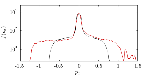
Figure 11: (color online) Space-integrated (over all $x$) longitudinal momentum distribution $f(p_{x})$ at $t=15\,\tau_{L}$ for $a_{0}=15$, $n_{0}=7$ and $\tau_{r}=0.25\,\tau_{L}$ (red, solid curve), $\tau_{r}=4\,\tau_{L}$ (black, dotted curve). Both cases correspond to total reflection. The central peak corresponds to the plasma bulk.

In Fig. 12, we moreover compare the front propagation velocity, $v_{f}$, for two sets of simulations with rise times $\tau_{r}=0.25\tau_{L}$ and $\tau_{r}=4\tau_{L}$. The front propagation speed $v_{f}$ is determined by the slope of the curves $x_{b}(t)$, see Fig. 4. We have studied cases of propagation for different $a_{0}$ and $n_{0}$ close to the threshold predicted by cold-fluid theory, for which $v_{f}$ ranges from $10^{-3}\,c$ up to $0.25\,c$, see Fig. 12. Within the error bars for the transparency threshold, $v_{f}$ takes values too small to reliably indicate propagation (i.e. beyond the accuracy permitted by our spatial and temporal resolution). As Fig. 12 shows, the propagation velocity $v_{f}$ for the same $a_{0}$ and $n_{0}$ is generally lower for the pulse with the larger rise time, $\tau_{r}=4\,\tau_{L}$. Nevertheless, for higher $a_{0}$, $v_{f}$ is far from negligible for densities lying well above the cold-fluid threshold, even for the case with larger rise time.

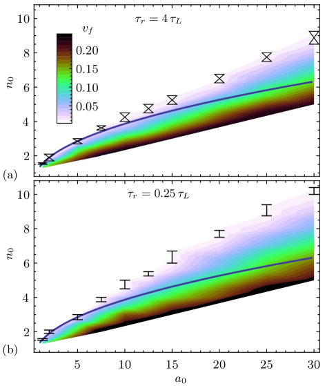
Figure 12: (color online) Front velocity $v_{f}$ as measured from PIC simulations with two different pulse rise times, (a) $\tau_{r}=4\,\tau_{L}$, (b) $\tau_{r}=0.25\,\tau_{L}$. The blue, solid line and error bars are the same as described in the caption of Fig. 1(a). The lower density range of simulations performed for a given $a_{0}$ has been set to improve readability.

V Discussion and conclusions

The relativistic, cold-fluid, stationary solutions of Refs. Marburger and Tooper (1975); Cattani et al. (2000); Goloviznin and Schep (2000) provide a convenient starting point to investigate the threshold of RSIT, even in the presence of longitudinal electron heating. While the fields inside the plasma clearly differ from the predictions of cold fluid theory, the fields in the CSL and vacuum are rather insensitive to density fluctuations within the plasma. Therefore, the dynamics of a test electron in the CSL or the vacuum can be accurately described using the fields of the stationary problem. This finding allows us to specify separatrices of bounded and unbounded motion for single electron dynamics, encapsulating the competition of ponderomotive and electrostatic forces at the edge of the plasma.

We have shown that one can define a critical momentum $|p_{x}^{\mathrm{cr}}|$, Eq. (43), or value of the Hamiltonian $H^{\mathrm{cr}}$, Eq. (44), corresponding to the separatrix which delimits oscillatory motion around the equilibrium position at the edge of the CEL. When a sufficiently high number of electrons at the edge of the CEL have $|p_{x}|>|p_{x}^{\mathrm{cr}}|$ and escape to the vacuum, RSIT occurs. In this work, we did not focus on the mechanism that provides momentum to electrons, i.e. we did not attempt to provide a model for the collisionless heating mechanism. We did however show, through our numerical study of the impact of the pulse rise time, that the pulse shape crucially affects longitudinal heating and that stronger heating results in a higher threshold density for RSIT. A detailed model for electron heating, which would allow us to predict $|p_{x}^{\mathrm{min}}|$ rather than infer it from PIC simulations, as done in Fig. 10, will be pursued elsewhere. We stress that, although in more realistic scenarios of laser-plasma interaction the actual heating at the plasma boundary would depend on several factors (see Ref. Sanz et al. (2012) for a recent study), the basic mechanism of electron escape into the vacuum at high enough momentum is expected to be the same.

In summary, we have used a dynamical systems approach to bridge the cold-fluid and kinetic levels of RSIT description. Deviations of PIC simulations from cold-fluid theory predictions are explained as a longitudinal heating effect induced by the incident laser pulse. The pulse temporal profile clearly affects electron heating and through it the threshold of RSIT. While there are several experimental works addressing RSIT in the case of linearly polarized laser pulses  Giulietti et al. (1997); Fuchs et al. (1998); Willingale et al. (2009); Palaniyappan et al. (2012), to the best of our knowledge the verification of RSIT for CP light remains elusive. We hope that our results trigger further investigations in this domain, as the reported dependency of the RSIT threshold on the pulse profile could provide a versatile tool for high-contrast CP laser pulse characterization.

VI Acknowledgments

We would like to thank A. Debayle, L. Gremillet, A. Macchi and A. Pukhov for helpful comments.

References

- Note (1) The definition of the vector potential is given in Eq. (3).
- Akhiezer and Polovin (1956) A. I. Akhiezer and R. V. Polovin, Sov. Phys. JETP 3, 915 (1956).
- Kaw and Dawson (1970) P. Kaw and J. Dawson, Phys. Fluids 13, 472 (1970).
- Klimo et al. (2008) O. Klimo, J. Psikal, J. Limpouch, and V. T. Tikhonchuk, Phys. Rev. ST Accel. Beams 11, 031301 (2008).
- Robinson et al. (2008) A. P. L. Robinson, M. Zepf, S. Kar, R. G. Evans, and C. Bellei, New J. Phys. 10, 013021 (2008).
- Yan et al. (2008) X. Q. Yan, C. Lin, Z. M. Sheng, Z. Y. Guo, B. C. Liu, Y. R. Lu, J. X. Fang, and J. E. Chen, Phys. Rev. Lett. 100, 135003 (2008).
- Macchi et al. (2009) A. Macchi, S. Veghini, and F. Pegoraro, Phys. Rev. Lett. 103, 085003 (2009).
- Grech et al. (2011) M. Grech, S. Skupin, A. Diaw, T. Schlegel, and V. T. Tikhonchuk, New J. Phys. 13, 123003 (2011).
- Naumova et al. (2009) N. Naumova, T. Schlegel, V. T. Tikhonchuk, C. Labaune, I. V. Sokolov, and G. Mourou, Phys. Rev. Lett. 102, 025002 (2009).
- Schlegel et al. (2009) T. Schlegel, N. Naumova, V. T. Tikhonchuk, C. Labaune, I. V. Sokolov, and G. Mourou, Phys. Plasmas 16, 083103 (2009).
- Yin et al. (2006) L. Yin, B. J. Albright, B. M. Hegelich, and J. C. Fernández, Laser Part. Beams 24, 291 (2006).
- Albright et al. (2007) B. J. Albright, L. Yin, K. J. Bowers, B. M. Hegelich, K. A. Flippo, T. J. T. Kwan, and J. C. Fernandez, Phys. Plasmas 14, 094502 (2007).
- Yin et al. (2011) L. Yin, B. J. Albright, K. J. Bowers, D. Jung, J. C. Fernández, and B. M. Hegelich, Phys. Rev. Lett. 107, 045003 (2011).
- Max and Perkins (1971) C. Max and F. Perkins, Phys. Rev. Lett. 27, 1342 (1971).
- Marburger and Tooper (1975) J. H. Marburger and R. F. Tooper, Phys. Rev. Lett. 35, 1001 (1975).
- Lai (1976) C. S. Lai, Phys. Rev. Lett. 36, 966 (1976).
- Cattani et al. (2000) F. Cattani, A. Kim, D. Anderson, and M. Lisak, Phys. Rev. E 62, 1234 (2000).
- Goloviznin and Schep (2000) V. V. Goloviznin and T. J. Schep, Phys. Plasmas 7, 1564 (2000).
- Eremin et al. (2010) V. I. Eremin, A. V. Korzhimanov, and A. V. Kim, Phys. Plasmas 17, 043102 (2010).
- Wilks et al. (1993) S. Wilks, W. Kruer, and W. Mori, IEEE T. Plasma Sci. 21, 120 (1993).
- Lefebvre and Bonnaud (1995) E. Lefebvre and G. Bonnaud, Phys. Rev. Lett. 74, 2002 (1995).
- Guérin et al. (1996) S. Guérin, P. Mora, J. C. Adam, A. Héron, and G. Laval, Phys. Plasmas 3, 2693 (1996).
- Sakagami and Mima (1996) H. Sakagami and K. Mima, Phys. Rev. E 54, 1870 (1996).
- Gibbon (2005) P. Gibbon, Short Pulse Laser Interactions with Matter (Imperial College Press, London, 2005).
- Note (2) Equation (12) then implies , as .
- Note (3) The difference corresponds to the number of equilibria in the CSL, which is a priori unknown.
- Lichtenberg and Lieberman (1992) A. J. Lichtenberg and M. A. Lieberman, Regular and Chaotic Dynamics (Springer, New York, 1992).
- Birdsall and Langdon (1991) C. Birdsall and A. Langdon, Plasma Physics Via Computer Simulation (Adam-Hilger, Bristol, UK, 1991).
- Grech et al. (2012) M. Grech, E. Siminos, and S. Skupin, (2012), in preparation.
- Taflove and Hagness (2005) A. Taflove and S. C. Hagness, Computational Electrodynamics: The Finite-Difference Time-Domain Method, 3rd ed. (Artech House, Norwood, MA, 2005).
- Boris (1970) J. Boris, in Proc. Fourth Conf. on Numerical Simulation of Plasmas (Naval Res. Lab, Washington, D.C., 1970) pp. 3–67.
- Esirkepov (2001) T. Esirkepov, Comput. Phys. Commun. 135, 144 (2001).
- Sanz et al. (2012) J. Sanz, A. Debayle, and K. Mima, Phys. Rev. E 85, 046411 (2012).
- Giulietti et al. (1997) D. Giulietti, L. A. Gizzi, A. Giulietti, A. Macchi, D. Teychenné, P. Chessa, A. Rousse, G. Cheriaux, J. P. Chambaret, and G. Darpentigny, Phys. Rev. Lett. 79, 3194 (1997).
- Fuchs et al. (1998) J. Fuchs, J. C. Adam, F. Amiranoff, S. D. Baton, P. Gallant, L. Gremillet, A. Héron, J. C. Kieffer, G. Laval, G. Malka, J. L. Miquel, P. Mora, H. Pépin, and C. Rousseaux, Phys. Rev. Lett. 80, 2326 (1998).
- Willingale et al. (2009) L. Willingale, S. R. Nagel, A. G. R. Thomas, C. Bellei, R. J. Clarke, A. E. Dangor, R. Heathcote, M. C. Kaluza, C. Kamperidis, S. Kneip, K. Krushelnick, N. Lopes, S. P. D. Mangles, W. Nazarov, P. M. Nilson, and Z. Najmudin, Phys. Rev. Lett. 102, 125002 (2009).
- Palaniyappan et al. (2012) S. Palaniyappan, B. M. Hegelich, H.-C. Wu, D. Jung, D. C. Gautier, L. Yin, B. J. Albright, R. P. Johnson, T. Shimada, S. Letzring, D. T. Offermann, J. Ren, C. Huang, R. Hörlein, B. Dromey, J. C. Fernandez, and R. C. Shah, Nature Phys. 8, 763 (2012).