Quantum and classical chaos of a two-electron system in a quantum wire

Abstract

We study classical and quantum dynamics of two spinless particles confined in a quantum wire with repulsive or attractive Coulomb interaction. The interaction induces irregular dynamics in classical mechanics, which reflects on the quantum properties of the system in the energy level statistics (the signatures of quantum chaos). We investigate especially closer correspondence between the classical and quantum chaos. The present classical dynamics has some scaling property, which the quantum counterpart does not have. However, we demonstrate that the energy level statistics implies the existence of the corresponding scaling property even in the quantum system. Instead of ordinary maximum Lyapunov exponent (MLE), we introduce a novel kind of MLE, which is shown to be suitable measure of chaotic irregularity for the present classical system. We show that tendency of the energy dependence of the Brody parameter, which characterizes the energy level statistics in the quantum system, is consistent with that of the novel kind of MLE.

I Introduction

The recent development in high technology has fabricated nano-scale quantum dots containing a finite number of interacting electrons and optically trapped atoms where a finite number of interacting macroscopic particles are trapped in a small area. Quantum mechanics of these systems constitutes a topical subject. In such systems, the underlying classical motion is expected to play an important role. The nature of the classical motion, i.e. regular, mixed, or chaotic character, reflects on some of the quantum properties of the systems, particularly in the energy level statistics. In this context, a number of studies on the quantum chaos of systems containing a few electrons in quantum dots have been reported Ull ; Mez ; Ahn ; Ahn2 ; Ves ; Fen ; Dro ; Xav ; Saw . However, closer correspondence between the classical chaos and the quantum chaos in those systems has not been investigated well.

The simplest system among them would be the one-dimensional system Ves ; Fen . In this paper we are concerned with behavior of two particles interacting with each other via the repulsive or attractive Coulomb potential in a one-dimensional system and study the correspondence between the classical and quantum chaos in detail. According to Fendrik et. al. Fen , we introduce an effective Hamiltonian for a quantum wire, which reduces the original 3D system to the quasi-one-dimensional system. While its classical dynamics has some scaling property, the quantum counterpart has no such scaling property. We, however, show that the energy level statistics implies the existence of the corresponding scaling property even in the quantum system. This is demonstrated by calculations of the Brody parameter for distributions of the nearest neighbor level spacing (NNLS). This subject, scaling in quantum chaos, has been examined for some other systems, coupled harmonic or quartic oscillators Hal ; Zim ; Zen and the hydrogen atom in a magnetic field Win .

In order to clarify closer correspondence between the classical and quantum chaos, we introduce a novel kind of maximum Lyapunov exponent (MLE) instead of ordinary MLE. The ordinary MLE is a measure of the rate per unit of time for separation between two adjacent orbits while the new MLE is the one per unit of distance for separation between them. The new MLE is a suitable measure to compare chaotic irregularity among classical orbits with different energies. We show that tendency of the energy dependence of the Brody parameter is consistent with that of the new MLE. We further show that the area of a chaotic region in Poincaré maps are not a suitable measure of chaotic irregularity for the present system, while several authors showed that it is a suitable measure of the irregularity in other systems Win ; Ter ; Har .

This paper is organized as follows: In Sec.II, we construct a quasi-one-dimensional model of two electrons confined in a quantum wire. We introduce a new kind of MLE. In Sec.III, we explore the distribution of NNLS in wide range of energy and interaction strength. Then we examine the chaotic irregularity of the corresponding classical system with the use of the MLE and Poincaré maps. We clarify correspondence between the energy dependence of the distribution of NNLS and the chaotic irregularity in the classical counterpart. Summary and conclusion are given in Sec.IV

II Model and method

II.1 Quantum dynamics

We consider two spinless particles (two electrons or an electron-hole pair with the same mass) confined in a quantum wire. We assume a narrow parabolic confinement in the transversal directions ($x$ and $y$-directions), which are much narrower than a confinement in the longitudinal direction ($z$-direction). We consider a hard wall potential in z-direction. The particles are interacting with each other via the repulsive or attractive Coulomb potential. The Hamiltonian of the system is written as

$$H = \sum_{i=1,2}\Big{[}-\frac{\hbar^{2}}{2m}\left(\frac{\partial^{2}}{\partial x_{i}^{2}}+\frac{\partial^{2}}{\partial y_{i}^{2}}+\frac{\partial^{2}}{\partial z_{i}^{2}}\right)$$

$$+\frac{1}{2}m\omega^{2}(x_{i}^{2}+y_{i}^{2})\Big{]}$$

$$\pm\frac{e^{2}}{\sqrt{(x_{1}-x_{2})^{2}+(y_{1}-y_{2})^{2}+(z_{1}-z_{2})^{2}}}.$$

(1)

We assume that the particles occupy the lowest-energy state associated with the transverse motion, which is energetically well separated from the excited states. Then the two-particle wave function can be approximated as

$$\Psi(\bm{r}_{1},\bm{r}_{2})=\phi_{0}(x_{1})\phi_{0}(y_{1})\phi_{0}(x_{2})\phi_{0}(y_{2})\Phi(z_{1},z_{2}),$$

(2)

where $\phi_{0}(x)$ is the lowest energy eigenstate of a harmonic oscillator. The wave function $\Phi(z_{1},z_{2})$ satisfies the equation

$$H_{1D}\Phi(z_{1},z_{2})=E\Phi(z_{1},z_{2}),$$ (3)

where the effective Hamiltonian $H_{1D}$ is defined by

$$H_{1D}=-\frac{\hbar^{2}}{2m}\left(\frac{\partial^{2}}{\partial z_{1}^{2}}+\frac{\partial^{2}}{\partial z_{2}^{2}}\right)+V_{1D}(\left|z_{1}-z_{2}\right|).$$

(4)

$V_{1D}(z)$ is the effective potential given by

$$V_{1D}(z) =\pm e^{2}\int\frac{|\phi_{0}(x_{1})|^{2}|\phi_{0}(y_{1})|^{2}|\phi_{0}(x_{2})|^{2}|\phi_{0}(y_{2})|^{2}}{\sqrt{(x_{1}-x_{2})^{2}+(y_{1}-y_{2})^{2}+z^{2}}}dx_{1}dy_{1}dx_{2}dy_{2}$$

$$=\pm\frac{e^{2}}{a}\int_{0}^{\infty}\frac{s\exp[-s^{2}/2]}{\sqrt{s^{2}+(z/a)^{2}}}ds$$ (5)

and $a=\sqrt{\hbar/m\omega}$. In this way, our system exhibits a quasi-one-dimensional property. Now we introduce a model potential Fen defined by

$$V_{m}(z)=\pm\frac{e^{2}}{\sqrt{a^{2}+z^{2}}}.$$ (6)

In Fig.1, the solid and broken curves indicate the numerically calculated potential $V_{1D}$ and the analytical potential $V_{m}$, respectively. We see that $V_{1D}$ can be well approximated by $V_{m}$. We adopt $V_{m}$ instead of $V_{1D}$ as the interaction potential between particles since the analytical potential can be dealt with more easily. Thus our effective Hamiltonian is written as

$$H_{eff} = -\frac{\hbar^{2}}{2m}\Big{(}\frac{\partial^{2}}{\partial z_{1}^{2}}+\frac{\partial^{2}}{\partial z_{2}^{2}}\Big{)}$$ (7)

$$\pm\frac{e^{2}}{\sqrt{a^{2}+(z_{1}-z_{2})^{2}}}.$$

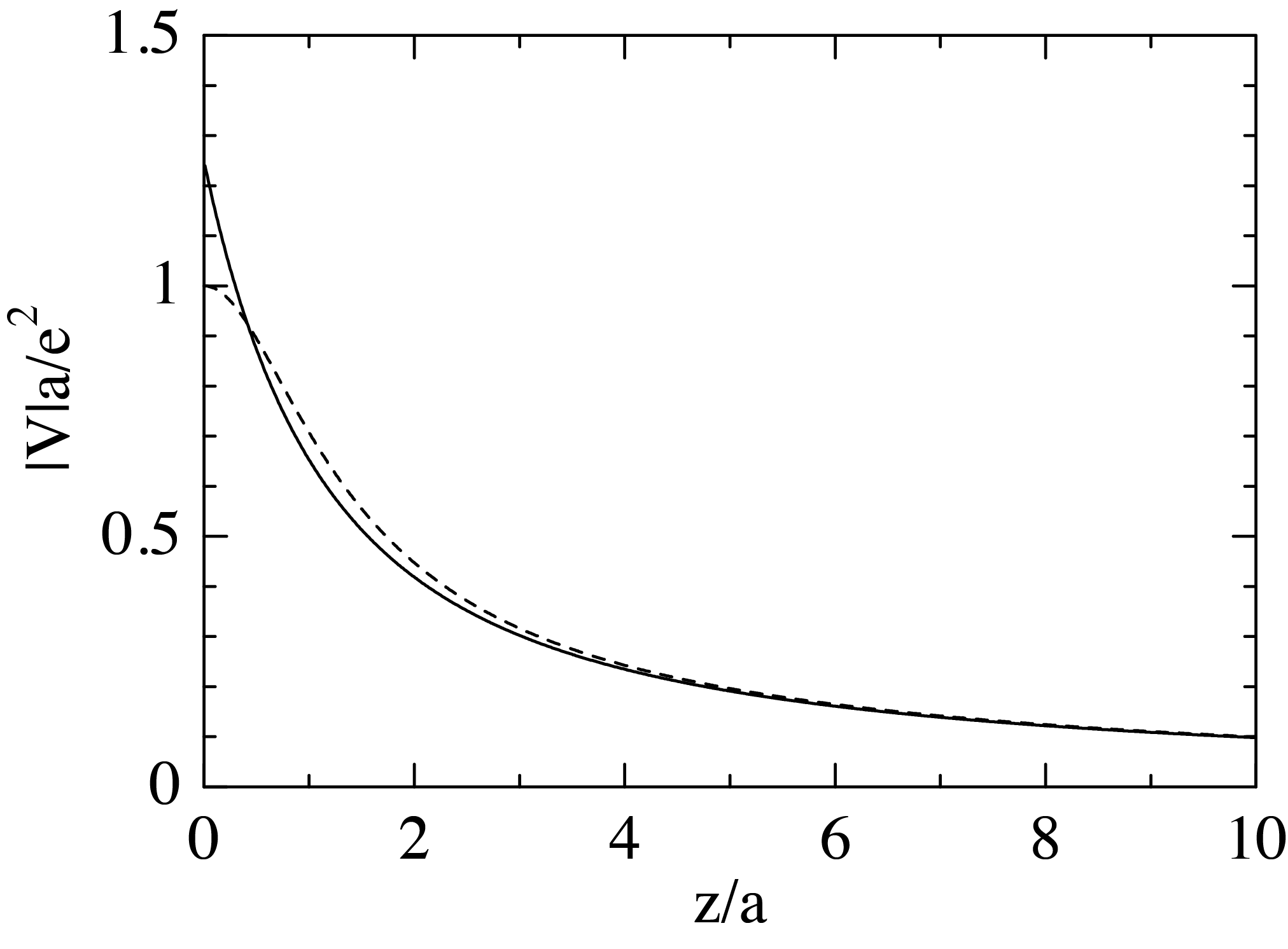
Figure 1: The numerically calculated potential $V_{1D}$ (solid curve) and the analytical potential $V_{m}$ (broken curve). The lengths and potentials are scaled by $a$ and $e^{2}/a$, respectively.

We scale lengths, angular momentums and masses by $L$, $\hbar$ and $2m$, respectively, where $L$ is a width of the system in the longitudinal direction. Then the effective Hamiltonian is reduced to

$$H_{eff}=-\left(\frac{\partial^{2}}{\partial z_{1}^{2}}+\frac{\partial^{2}}{\partial z_{2}^{2}}\right)+\frac{\lambda}{\sqrt{(z_{1}-z_{2})^{2}+\delta^{2}}},$$

(8)

where $\lambda$ is the effective interaction strength parameter given by $\lambda=\pm 2e^{2}mL/\hbar^{2}$ and $\delta=a/L$. Note that the parameter $\lambda$ can be expressed as $\lambda=\pm 2L/a_{B}$, where $a_{B}$ is the Bohr radius defined by $a_{B}=\hbar^{2}/e^{2}m$. The particles are confined by hard walls within $0\leq z_{1}\leq 1$ and $0\leq z_{2}\leq 1$. These hard walls describe the boundary of the quasi-one-dimensional wire. We examine the feature of the system as varying $\lambda$ while keeping $\delta$, which implies that we vary the system size keeping the ratio between the longitudinal and transversal lengths.

It should be noted that the present 1D two-particle system is equivalent to a 2D system of one particle having a coordinate $(z_{1},z_{2})$ within a hard-walled square billiard. The Hamiltonian of the latter system is also given by Eq.(8), in which the first and second terms represent the kinetic energy of the particle and the third term represents a external potential. We can chose energy eigenfunctions of the 2D system as being symmetric or antisymmetric against exchange between $z_{1}$ and $z_{2}$, i.e., $\Phi(z_{1},z_{2})=\Phi(z_{2},z_{1})$ or $\Phi(z_{1},z_{2})=-\Phi(z_{2},z_{1}),$ since the Hamiltonian does not change under this exchange. The symmetric and antisymmetric cases correspond to the boson and fermion cases, respectively, in the 1D two-particle system. In the present paper we are concerned only with the cases of fermions.

In order to look for signatures of quantum chaos in the present system, we examine distributions of the nearest neighbor level spacing (NNLS). The eigenenergies are obtained by diagonalizing the Hamiltonian matrices numerically, whose elements are evaluated by using energy eigenstates without the Coulomb interaction (Slater determinants) as a basis set:

$$\phi_{m,n}(z_{1},z_{2}) = \sqrt{2}\Big{(}\sin(m\pi z_{1})\sin(n\pi z_{2})$$ (9)

$$-\sin(n\pi z_{1})\sin(m\pi z_{2})\Big{)},$$

where $m$ and $n$ are integer larger than zero. The components of the Hamiltonian matrices are represented with respect to $\phi_{m,n}$ in Eq.(9) as

$$<\phi_{m,n}|H|\phi_{m^{\prime},n^{\prime}}>=\pi^{2}(m^{2}+n^{2})\delta_{m,m^{\prime}}\delta_{n,n^{\prime}}$$

$$\hskip 5.69046pt+4\lambda\{I(m,n|m^{\prime},n^{\prime})-I(m,n|n^{\prime},m^{\prime})\},$$ (10)

where $I(m,n|m^{\prime},n^{\prime})$ is defined by

$$I(m,n|m^{\prime},n^{\prime})=\int_{0}^{1}\int_{0}^{1}dz_{1}dz_{2}\frac{\sin(m\pi z_{1})\sin(n\pi z_{2})\sin(m^{\prime}\pi z_{1})\sin(n^{\prime}\pi z_{2})}{\sqrt{(z_{1}-z_{2})^{2}+\delta^{2}}}.$$

We further take into account the parity of the system. The present system is invariant under the inversion associated with the center $(z_{1},z_{2})=(1/2,1/2)$. Therefore, the eigenstates are classified into ones having the even parity with $(m,n)=$(even, even) or (odd, odd) and those having odd parity with $(m,n)=$(even, odd) or (odd, even). We concentrate ourselves on the eigenstates of the even parity in this paper, when we examine NNLS.

NNLS is fitted to the Brody distribution function

$$P_{B}(S) = (\alpha+1)bS^{\alpha}\exp(-bS^{\alpha+1}),$$

$$b = \Big{\{}\Gamma\Big{(}\frac{\alpha+2}{\alpha+1}\Big{)}\Big{\}}^{\alpha+1},$$ (12)

which interpolates the Poisson and Wigner distributions. It coincides with the Poisson distribution for $\alpha=0$ and recovers the Wigner distribution for $\alpha=1$. We use the Brody parameter $\alpha$ as a measure for degree of chaotic irregularity of the system.

II.2 Classical dynamics

Now we turn to the dynamics of the classical counterpart of the two-particle system described by the Hamiltonian (8) . Similarly to the quantum case, lengths, angular momentums and masses are scaled by $L$, $\hbar$ and $2m$, respectively. The equations of the motion are then given as

$$\frac{1}{2}\frac{d^{2}z_{1}}{dt^{2}}=\frac{\lambda(z_{1}-z_{2})}{\{(z_{1}-z_{2})^{2}+\delta^{2}\}^{3/2}},$$

$$\frac{1}{2}\frac{d^{2}z_{2}}{dt^{2}}=\frac{\lambda(z_{2}-z_{1})}{\{(z_{1}-z_{2})^{2}+\delta^{2}\}^{3/2}}.$$ (13)

The $\lambda$ defined by $\lambda=\pm 2e^{2}mL/\hbar^{2}$ is dimensionless. The total energy is represented as

$$E = \frac{1}{4}\Big{(}\frac{dz_{1}}{dt}\Big{)}^{2}+\frac{1}{4}\Big{(}\frac{dz_{2}}{dt}\Big{)}^{2}$$ (14)

$$+\frac{\lambda}{\sqrt{(z_{1}-z_{2})^{2}+\delta^{2}}}.$$

The dynamics of the present system is equivalent to that of a particle confined in a two-dimensional square box in $0\leq z_{1}\leq 1$ and $0\leq z_{2}\leq 1$ with the potential $\lambda/\sqrt{(z_{1}-z_{2})^{2}+\delta^{2}}$ similarly to the quantum case. The behavior of the system apparently depends on the interaction strength parameter $\lambda$. However, if we introduce a rescaled time $\tau$ defined by $\tau=\sqrt{|\lambda|}t$, the equations of the motion are reduced to

$$\frac{1}{2}\frac{d^{2}z_{1}}{d\tau^{2}}=\pm\frac{(z_{1}-z_{2})}{\{(z_{1}-z_{2})^{2}+\delta^{2}\}^{3/2}},$$

$$\frac{1}{2}\frac{d^{2}z_{2}}{d\tau^{2}}=\pm\frac{(z_{2}-z_{1})}{\{(z_{1}-z_{2})^{2}+\delta^{2}\}^{3/2}}.$$ (15)

The rescaled energy $\varepsilon=E/|\lambda|$ is given by

$$\varepsilon = \frac{1}{4}\Big{(}\frac{dz_{1}}{d\tau}\Big{)}^{2}+\frac{1}{4}\Big{(}\frac{dz_{2}}{d\tau}\Big{)}^{2}$$ (16)

$$\pm\frac{1}{\sqrt{(z_{1}-z_{2})^{2}+\delta^{2}}}.$$

The plus and minus signs in Eqs.(15) and (16) correspond to positive and negative $\lambda$, respectively. Consequently, the classical behavior of the system is independent of the value of $\lambda$ itself. This is because in the classical system there is no such characteristic length as the Bohr radius due to the finite Plank constant in the quantum system. Even if we enlarge the system size, we can find the equivalent trajectory by increasing the total energy. On the other hand, the quantum behavior of the system depends on the value of $\lambda$ directly. Now the following question arises: Even in the quantum case, whether does the system with the same value of $E/|\lambda|$ but with different $\lambda$ exhibit a similar behavior to classical system, especially, concerning the degree of chaotic irregularity of the system? Otherwise there is no closer correspondence between the classical chaos and the quantum chaos. We investigate this point in the present study.

We use two kinds of the Poincaré map to see behavior of the classical system. The first kind of Poincaré map called Poincaré map 1 is defined in the section $v_{2}$ versus $z_{2}$ for the second particle taken at times when the first particle bounces off the left boundary of the well $(z_{1}=0)$. The second kind of Poincaré map called Poincaré map 2 is defined as follows. We take coordinate $l$ along the two sides of the square and a diagonal line connecting $(z_{1},z_{2})=(0,0)$ and $(1,1)$ where the ridge of the potential lies (see Fig.2). $l$ is normalized so that the range is $0\leq l\leq 1$. The trajectory can be recorded by two values. One is $l$ at point where the particle is reflected on the hardwalls or intersects the line $z_{1}=z_{2}$. The other is $p=\cos\theta$, where $\theta$ is the angle between the velocity vector after reflection and the normal to the solid line. The Poincaré map which records $l$ and $\theta$ of orbits reflects the property of the classical system.

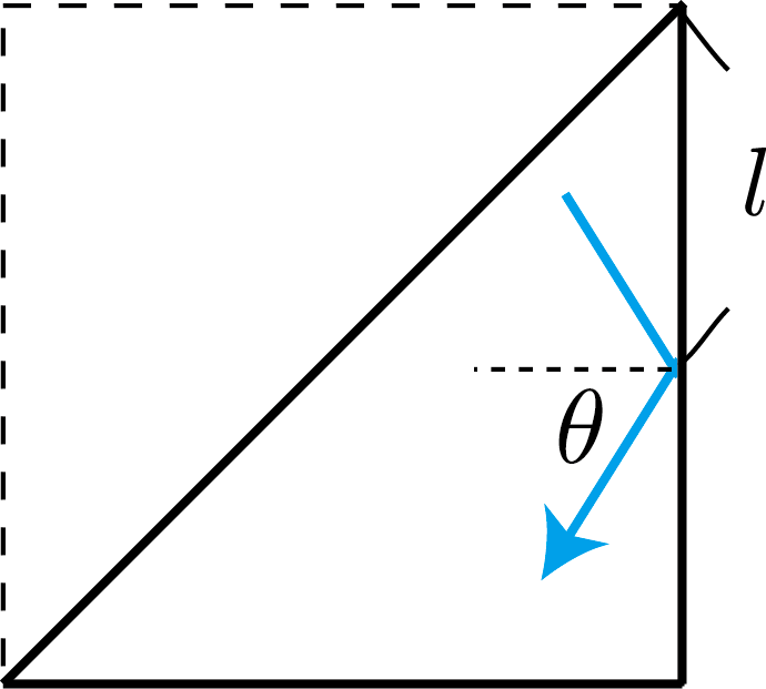
Figure 2: The coordinates of the billiard system.

We also use MLE as a measure for degree of chaotic irregularity of the classical system. The ordinary Lyapunov exponent is defined as follows: we consider an orbit $({\bf p}(\tau),{\bf q}(\tau))$ (denoted as the reference orbit) and a slightly displaced orbit from the reference orbit in the phase space. The starting point of the displaced orbit is spaced apart by a small vector $(\Delta{\bf p}(0),\Delta{\bf q}(0))$ from $({\bf p}(0),{\bf q}(0))$ at initial time $\tau=0$. The distance between the reference and displaced orbits is

$$d_{0}=|(\Delta{\bf p}(0),\Delta{\bf q}(0))|.$$ (17)

We follow these orbits for a time interval $\Delta\tau$. The distance between the two orbits at $\tau=\Delta\tau$ is represented as

$$d_{1}=|(\Delta{\bf p}(\Delta\tau),\Delta{\bf q}(\Delta\tau))|.$$ (18)

Then we choose a new starting point of displaced trajectory at time $\tau=\Delta\tau$ as

$$({\bf p}(\Delta\tau),{\bf q}(\Delta\tau))$$

$$\hskip 14.22636pt+\frac{d_{0}}{d_{1}}(\Delta{\bf p}(\Delta\tau),\Delta{\bf q}(\Delta\tau))$$ (19)

so that the distance between the new starting points equals $d_{0}$. The trajectory is followed up to time $\tau=2\Delta\tau$. The new deviation of the displaced orbit from the reference orbit

$$d_{2}=|(\Delta{\bf p}(2\Delta\tau),\Delta{\bf q}(2\Delta\tau))|$$ (20)

is computed, and a second rescaled trajectory is started. This process is continued, yielding a sequence of distances $d_{0},d_{1},d_{2},\cdots$. By using these values, MLE is defined as

$$\Gamma_{L}=\lim_{n\rightarrow\infty}\frac{1}{n\Delta\tau}\sum_{i=1}^{n}\ln\frac{d_{i}}{d_{0}},$$ (21)

where $n$ is the number of the time segment. This quantity $\Gamma_{L}$ is, however, not suitable as a measure for degree of chaotic irregularity in the present system. $\Gamma_{L}$ increases with $\varepsilon$ only even because the motion of particles becomes faster with the increase of $\varepsilon$, while the classical dynamics becomes regular in high energy regime as shown by the numerical results in the next section.

We introduce a novel kind of MLE defined as

$$\Gamma^{\prime}_{L}=\lim_{n\rightarrow\infty}\sum_{i=1}^{n}\frac{1}{n\xi}\ln\frac{d_{i}}{d_{0}}.$$ (22)

The definition of $\Gamma_{L}^{\prime}$ is almost the same as $\Gamma_{L}$ except that $\Delta\tau$ in Eq.(21) is replaced by a small distance $\xi$. The definition of $\Gamma^{\prime}_{L}$ in Eq.(22) is similar to Eq.(21). For $\Gamma_{L}^{\prime}$ we follow the two adjacent orbits while the reference orbit travels small distance $\xi$, and then evaluate $d_{i}$. $\Gamma^{\prime}_{L}$ represents the degree of exponential divergence of adjacent orbits similarly to $\Gamma_{L}$. However, $\Gamma^{\prime}_{L}$ depends only on geometry of orbits but not on quickness of development of orbits. We employ $\Gamma^{\prime}_{L}$ in Eq.(22) as a measure of degree of chaotic irregularity in classical mechanics.

III Numerical results

III.1 Repulsive interaction

We obtain energy eigenvalues by diagonalizing the effective Hamiltonian (8), and evaluate the smoothed counting function $N_{av}(E)$ which gives the cumulative number of states below an energy $E$. In order to analyze the structure of the level-fluctuation properties, we unfold the spectrum by applying the well-known transformation $x_{n}=N_{av}(E_{n})$ to obtain a constant mean spacing, where $n$ denotes the number of the energy level. From the unfolded spectrum we obtain the histogram of the NNLS distribution $P(S)$, where $S_{n}=x_{n+1}-x_{n}$. The histogram is fitted to the Brody distribution function $P_{B}(S)$ in Eq.(12). The integral of the Brody distribution function,

$$I_{B}(S)\equiv\int_{0}^{S}P_{B}(S^{\prime})dS^{\prime}$$ (23)

satisfies

$$\ln\ln[1/(1-I_{B}(S))]$$

$$\hskip 14.22636pt=(1+\alpha)\ln S+\ln b,$$ (24)

where $b$ is given in Eq.(12). By using the above relation and the least-squares fitting method we evaluate the Brody parameter $\alpha$ for the dstribution $P(S)$ of the NNLS. Hereafter we take $\delta=0.01$. As an example, a result of fitting for $\lambda=200$ is shown in Fig.3.

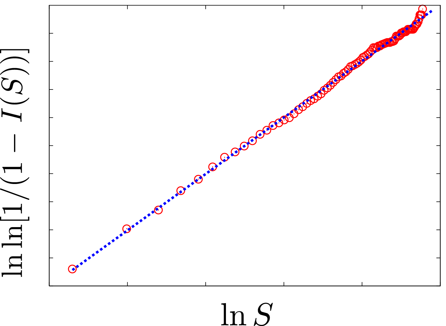
Figure 3: Relation between $\ln S$ and $\ln\ln[1/(1-I(S))]$ for $\lambda=200$ and $\delta=0.01$. $I(S)$ is the cumulative number of states in the unfolded spectrum. The NNLS is calculated by using the $1000$th eigenstate and following $1000$ eigenstates. The dotted line is obtained by using Eq.(24) and the least-squares fitting method .

The total energy region is divided into several regions. In Fig.4 we show the obtained NNLS distribution in each region for $\lambda=200$. About 1000 eigenvalues are used in each region to compute each histogram. The range of the used energy levels and the Brody parameter $\alpha$ are shown below each panel. We see that the Brody parameter decreases with increase of the average of energy eigenvalues which are used to obtain the histogram. Especially for the histograms in the panels (e) and (f) in Fig.4 with the Brody parameter less than $0.015$, the histograms are well fitted also by the Poisson distribution. The histograms for $\lambda=500$ is shown in Fig.5.

We see that the Brody parameter $\alpha$ decreases with increase of the average of energy eigenvalues similarly to the case of $\lambda=200$, and moreover that the values of $\alpha$ are greater than those for $\lambda=200$ in each energy level region.

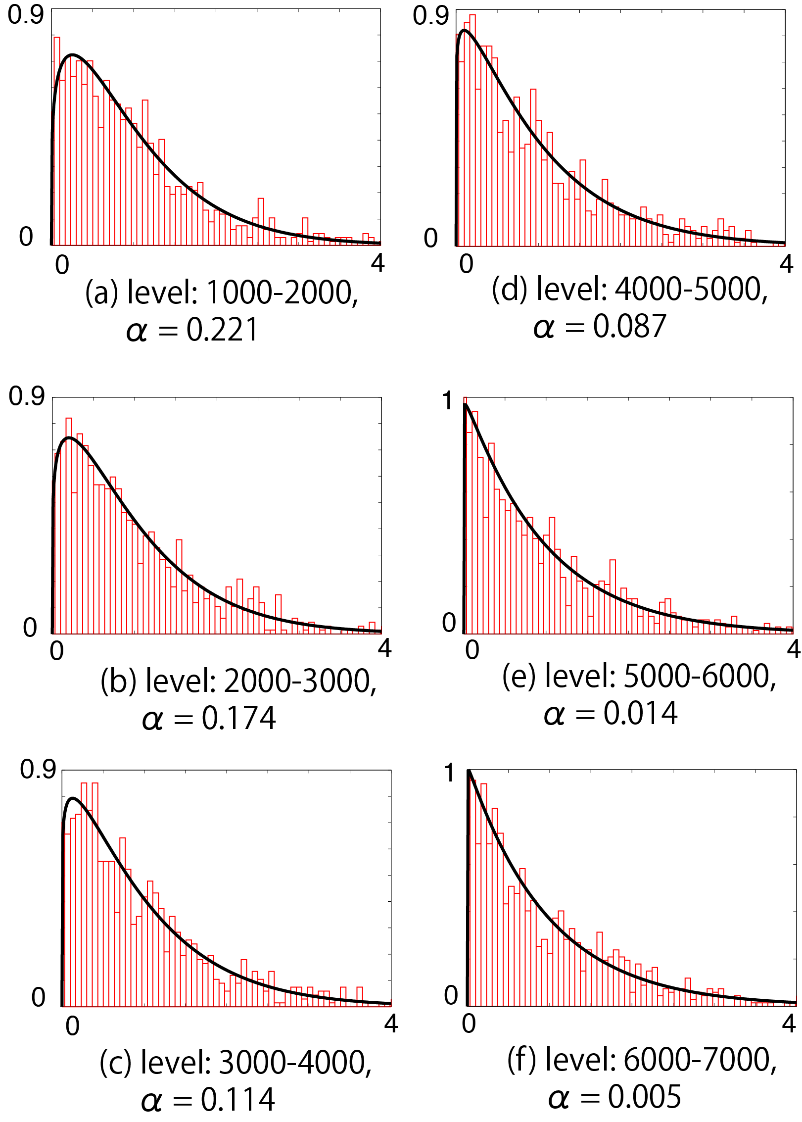
Figure 4: Histograms of NNLS for $\lambda=200$. Solid lines are the best fitted Brody distributions. Each value of the Brody parameter $\alpha$ is shown below each panel.

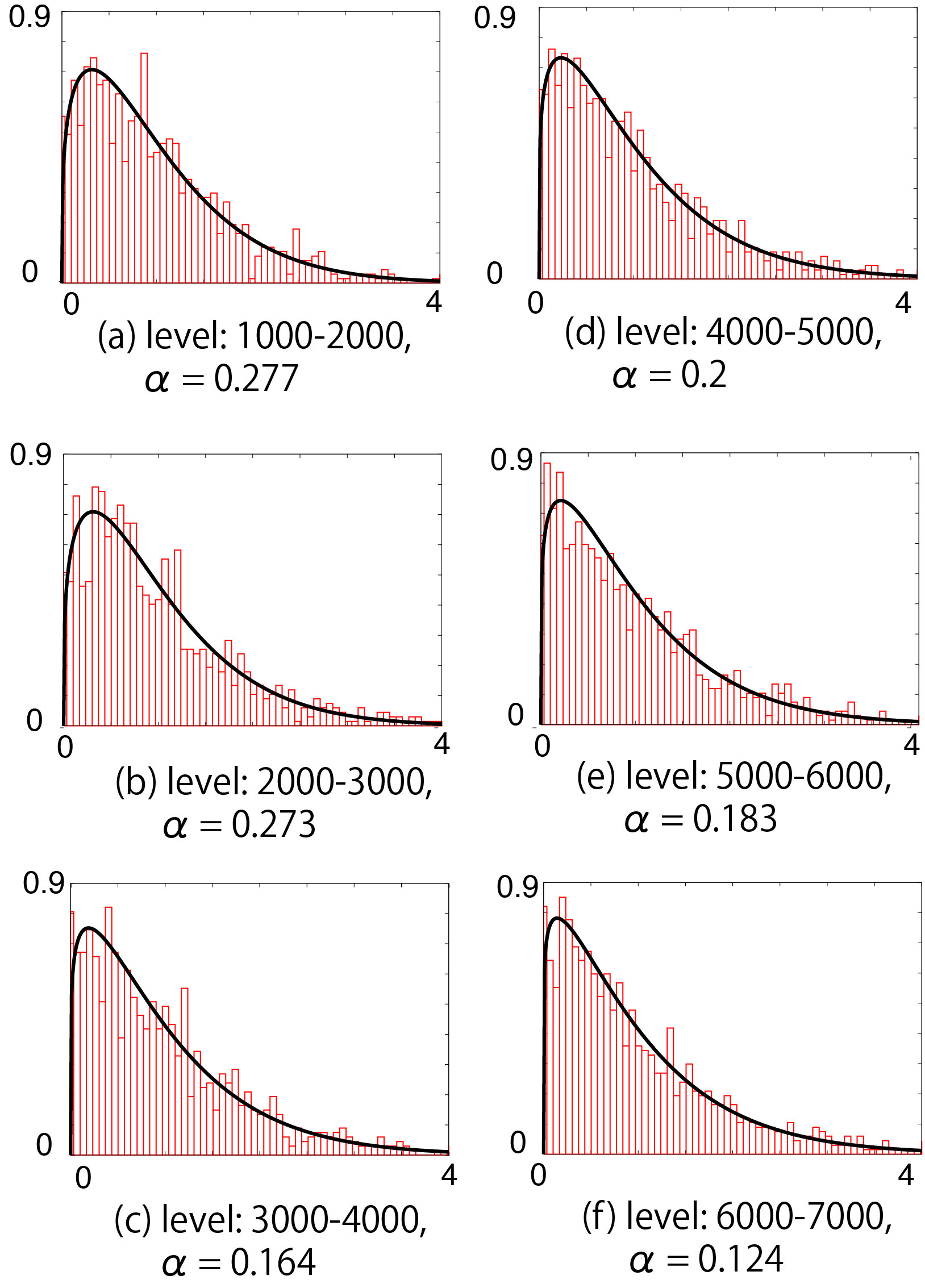
Figure 5: The same as Fig.4 except for $\lambda=500$.

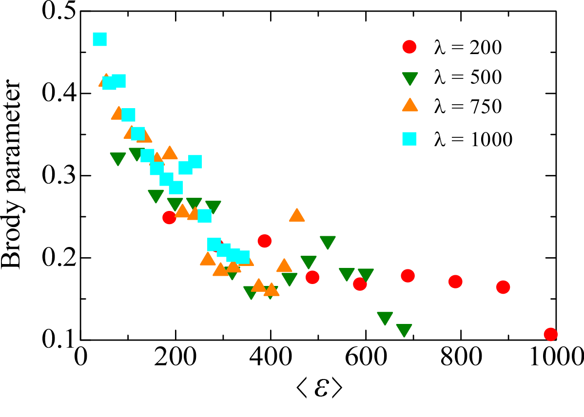
Figure 6: $\varepsilon-$dependence of the Brody parameter for the repulsive interaction. For each data point eigenvalues in the energy interval $\Delta E=50000$ were used (Their number is about 1000). Horizontal axis denotes the average of $\varepsilon$.

We show the $\varepsilon-$dependence of the Brody parameter for $\lambda=200,500,750,1000$ in Fig.6. For each data point we use energy eigenvalues in energy interval $\Delta E=50000$ which includes about $1000$ energy eigenvalues. The horizontal axis denotes the averaged value of $\varepsilon$ of the used eigenstates, $<\varepsilon>$. We see that the Brody parameter $\alpha$ decreases almost monotonously with increase of $<\varepsilon>$. Moreover the $\varepsilon-$dependences of $\alpha$ is quite similar for different $\lambda$ especially in $<\varepsilon><600$. As mentioned in the previous section, the classical system has scaling property characterized by parameter $\varepsilon=E/|\lambda|$. The above results indicate that the distribution of NNLS in quantum mechanics has the same scaling property on $\varepsilon$.

Now we see the behavior of the classical system with the equations of motion, Eq.(15). In Figs.7-9 we show the Poincaré maps 1 defined in previous section for $\varepsilon=50,200,1000$, respectively, with $\delta=0.01$. In Figs.10-12 the Poincaré maps 2 are shown. We have taken about 20 different initial points in phase space for each map. These Poincaré maps show that the present classical system exhibits mixed dynamics with coexisting KAM tri and chaotic regions. This is consistent with the fact that NNLS distributions in the quantum system are intermediate between the Poisson and Wigner distribution.

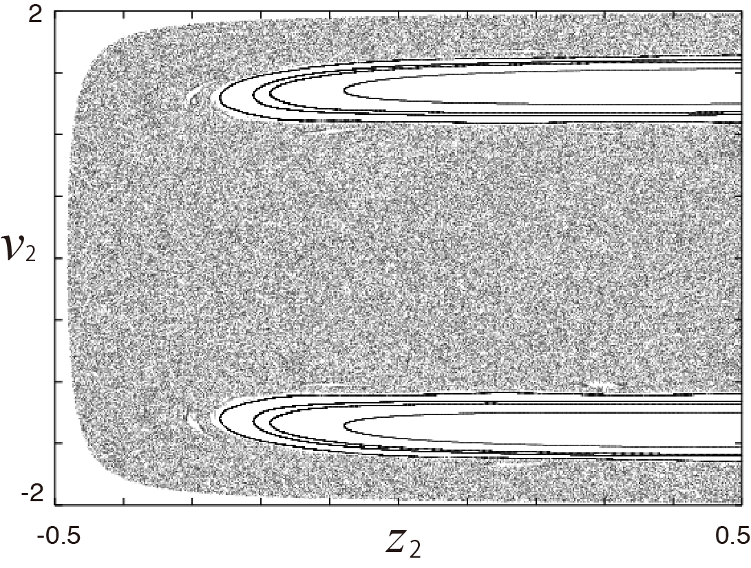
Figure 7: Poincaré map 1 for repulsive interaction with $\varepsilon=50$.

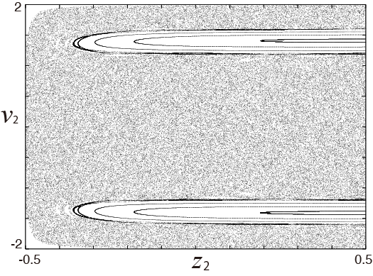
Figure 8: Poincaré map 1 for repulsive interaction with $\varepsilon=200$.

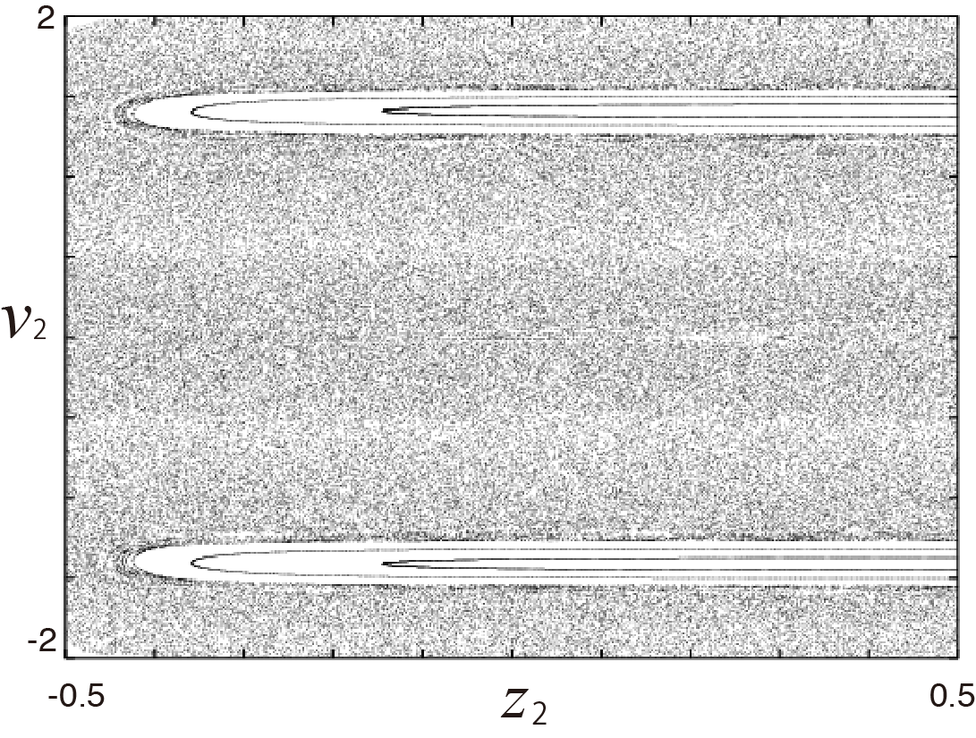
Figure 9: Poincaré map 1 for repulsive interaction with $\varepsilon=1000$.

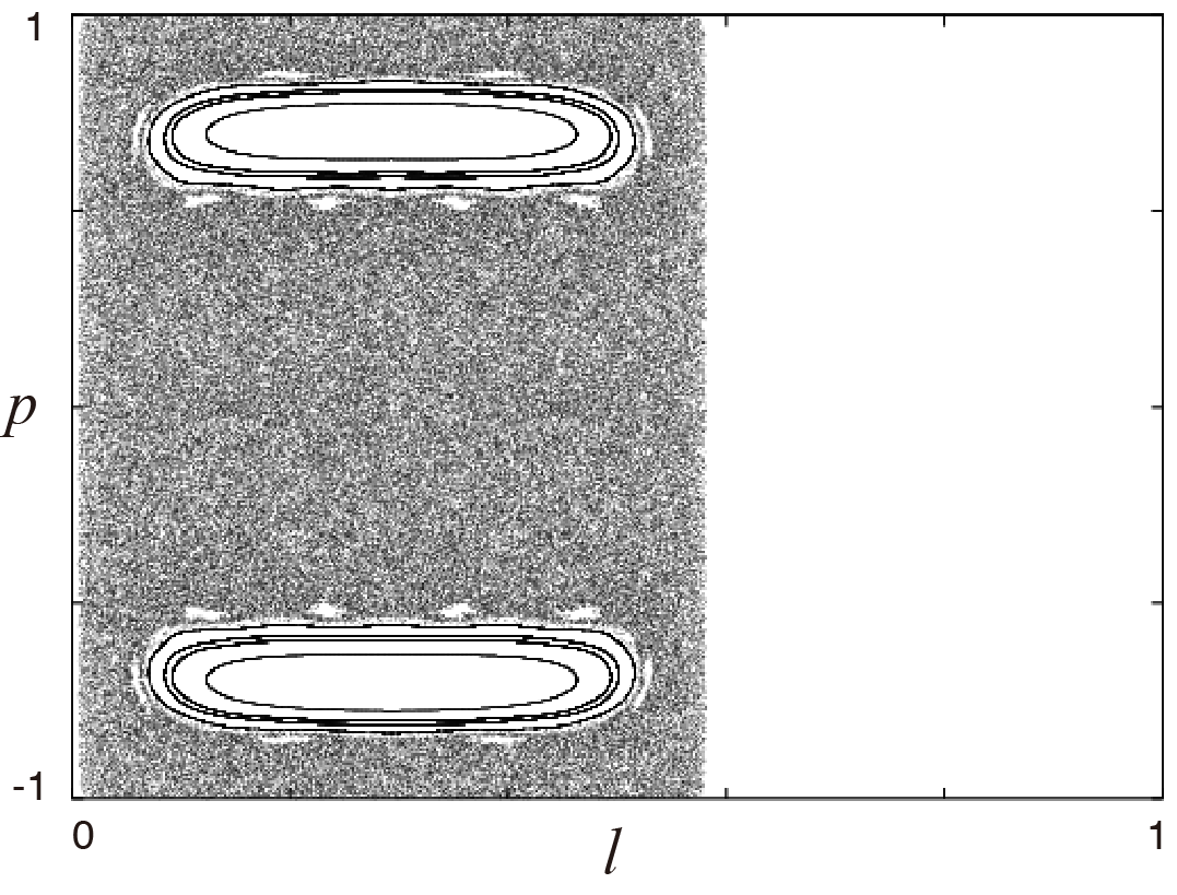
Figure 10: Poincaré map 2 for repulsive interaction with $\varepsilon=50$.

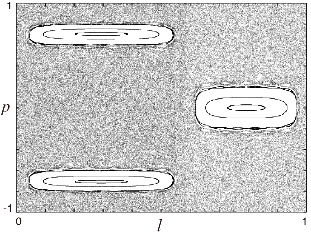
Figure 11: Poincaré map 2 for repulsive interaction with $\varepsilon=200$.

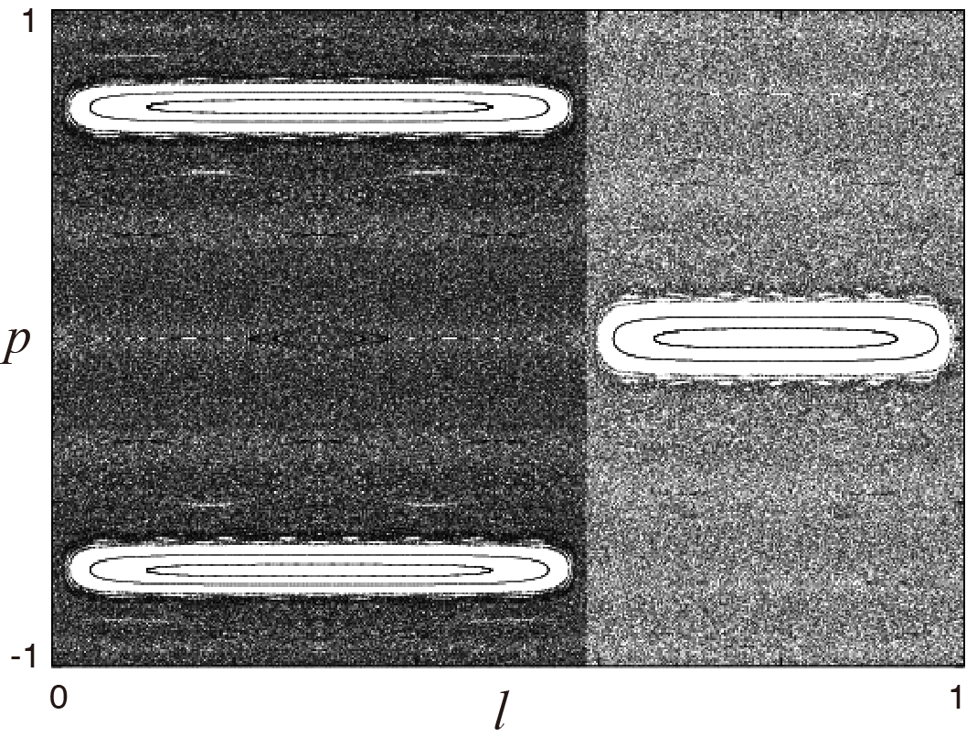
Figure 12: Poincaré map 2 for repulsive interaction with $\varepsilon=1000$.

In Fig.13 typical trajectories $(z_{1}(t),z_{2}(t))$ are shown for (a) $\varepsilon=50$,(b) $\varepsilon=200$ and (c) $\varepsilon=1000$, respectively. The Poincaré maps for those orbits show that they are chaotic. It is seen that the potential bends the trajectories especially near $z_{2}=z_{1}$ line for $\varepsilon=50$ and $\varepsilon=200$. It causes irregularity on the orbits. Contrastively the effect of potential is much less for $\varepsilon=1000$. The trajectory is composed of nearly straight lines. The orbits become more regular for larger $\varepsilon$ if $\varepsilon$ is large enough.

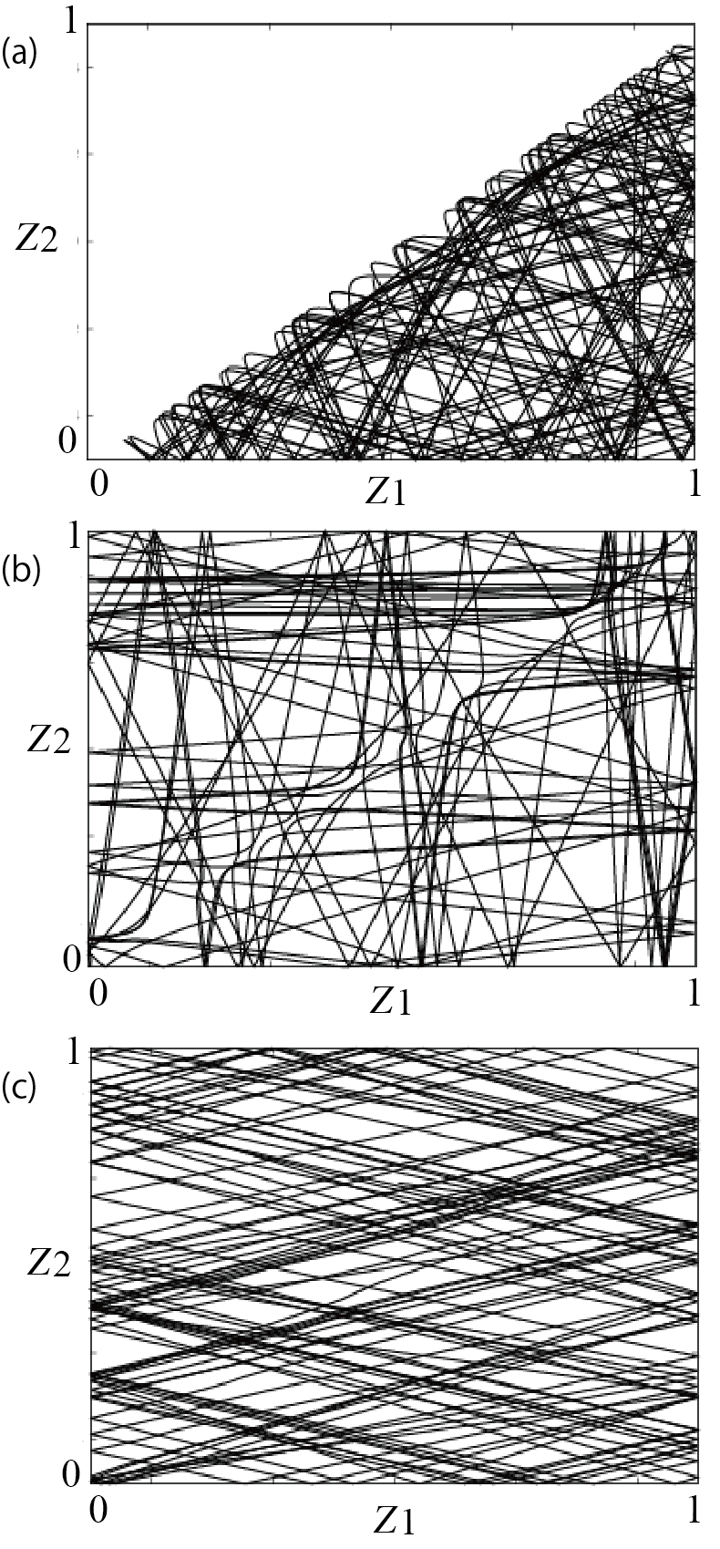
Figure 13: Typical trajectories $(z_{1}(t),z_{2}(t))$ with (a) $\varepsilon=50$,(b) $\varepsilon=200$, (c) $\varepsilon=1000$, respectively.

In order to confirm this point quantitatively we evaluate $\Gamma^{\prime}_{L}$ in Eq.(22) with $\xi=0.01$, which reflects irregularity of trajectories. Numerical calculation of each trajectory is performed for time more than $1.5\times 10^{5}$. We take the average of $\Gamma^{\prime}_{L}$ over about 20 orbits corresponding to the largest irregular region in the Poincaré maps for each $\varepsilon$. We show the $\varepsilon-$dependence of $\Gamma^{\prime}_{L}$ in Fig.14. The decrease of $\Gamma^{\prime}_{L}$ indicates the fact that the dynamics becomes more regular with the increase of $\varepsilon$, which is consistent with the above intuitive view from Fig.13. It is also consistent with the $\varepsilon-$dependence of $\alpha$ in the quantum system.

Figure 14: $\varepsilon-$dependence of $\Gamma_{L}^{\prime}$ in Eq.(22). The broken line is a guide to the eyes.

Now we calculate the ordinary MLE $\Gamma_{L}$ in Eq.(21) with $\Delta\tau=0.01$. Numerical calculations for trajectories are performed for time more than $1.5\times 10^{5}$. We take the average of $\Gamma_{L}$ over about 20 orbits corresponding to the largest irregular region in the Poincaré maps as well as for $\Gamma_{L}^{\prime}$. The $\varepsilon-$dependence of $\Gamma_{L}$ is shown in Fig.15. We see that $\Gamma_{L}$ increases with $\varepsilon$. This is because motions of the particles become faster with the increase of $\varepsilon$ and does not necessarily imply the increase of chaotic irregularity. Therefore $\varepsilon-$dependence of $\Gamma_{L}$ does not directly reflect the degree of chaotic irregularity.

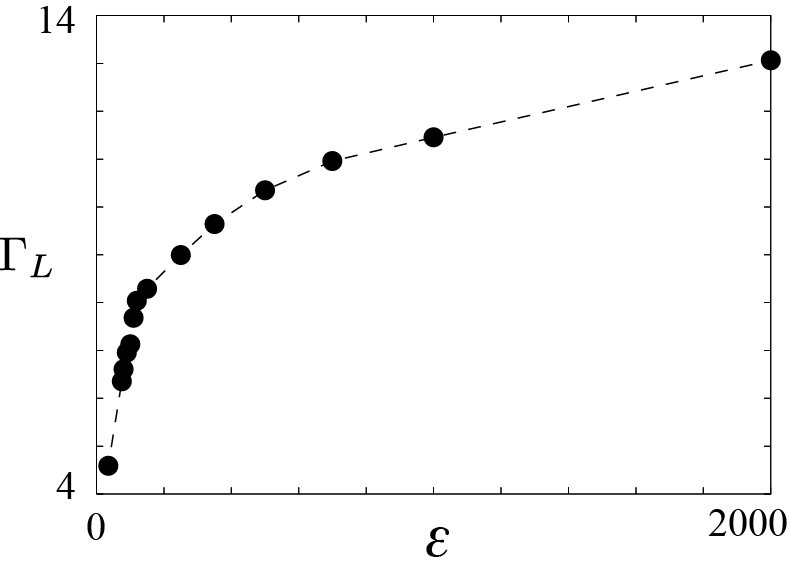
Figure 15: The same as Fig.14 except for $\Gamma_{L}$ in Eq.(21).

We also point out that an area of the largest irregular region in Poincaré map, which is adopted by several authors as a measure of chaotic irregularity Win ; Ter ; Har , is irrelevant for the present system. We calculate the ratio $R_{a}$ between two areas in Poincaré maps: the area of the largest irregular region and the area of total region reachable for a particle with $\varepsilon$. For the calculations we take meshes on Poincaré map. A total number of meshes is $300\times 300$. Then we count the number of meshes which an irregular trajectory visits and compare it to the total number of meshes energetically allowed. Numerical calculations of the trajectories are performed for time more than $2.0\times 10^{5}$. The $\varepsilon-$dependence of $R_{a}$ for Poincaré map 1 and 2 are shown in Figs.16 and 17, respectively. It is seen that $R_{a}$ increases with $\varepsilon$ for $\varepsilon>100$, in which the trajectory in two-dimensional square can cross the potential hill (the diagonal line). On the other hand, the orbits become more regular as seen obviously in Fig.13 when $\varepsilon$ increases for $\varepsilon>100$. Therefore $R_{a}$ is not a proper measure of irregularity in the present system in contrast to the other systems, in which $R_{a}$ can be adopted as a measure of irregularity Win ; Ter ; Har .

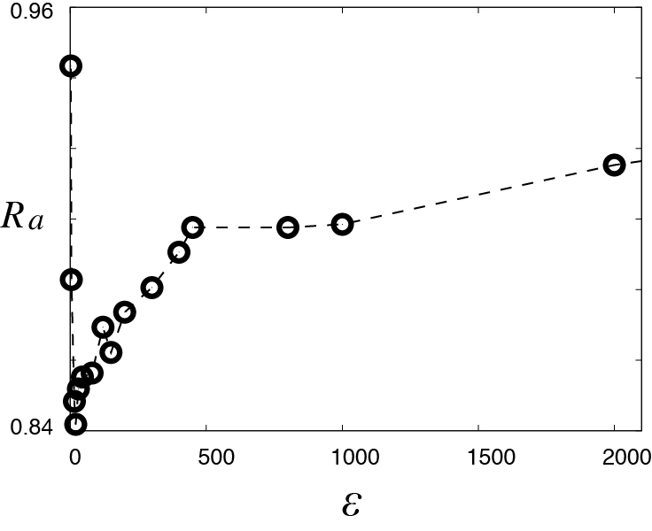
Figure 16: $\varepsilon-$dependence of the ratio $R_{a}$ between two areas in Poincaré map 1: the area of the largest irregular region and area of total region reachable for a particle with $\varepsilon$. The broken line is a guide to the eyes.

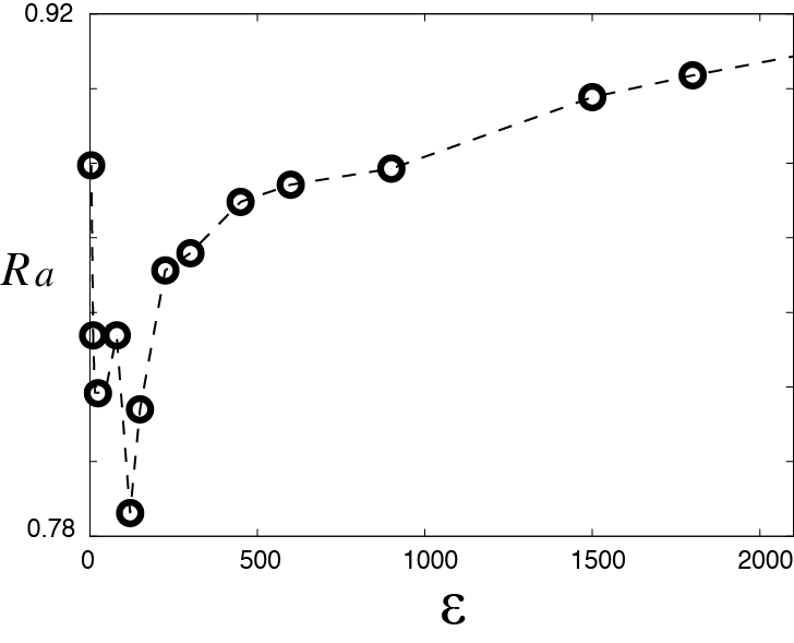
Figure 17: The same as Fig.16 except for Poincaré map 2.

III.2 Attractive interaction

Now we turn to results for the case of the attractive interaction with $\lambda<0$ and $\delta=0.01$. The $\varepsilon-$dependence of the Brody parameter is shown in Fig.18. $<\varepsilon>$ is the average of $\varepsilon$ of the used eigenstates. The decrease of the Brody parameter is seen with the increase of the scaled energy $\varepsilon$. We see that the Brody parameter depends almost only on $\varepsilon$ and not on $E$ and $\lambda$ separately, which is a situation similar to the case of the repulsive interaction.

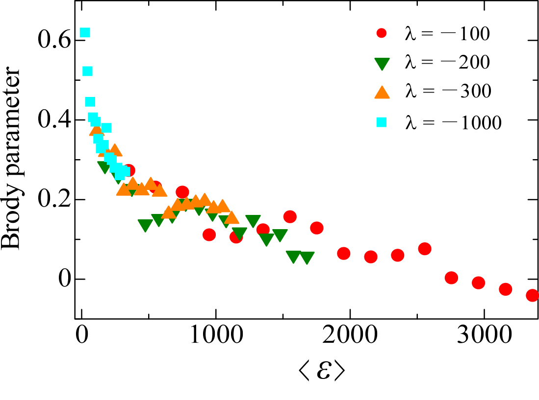
Figure 18: $\varepsilon-$dependence of the Brody parameter for the attractive interaction. For each data point eigenvalues in the energy interval $\Delta=50000$ were used ( The number of eigenvalues used to calculate each data point is about 1000). Horizontal axis denotes the average of $\varepsilon$ of the used eigenstates.

Next, we consider the corresponding classical dynamics described by the equations of motion in Eq.(15) for the attractive interaction. The Poincaré maps 1 are shown for $\varepsilon=5,200,1000$ in Figs.19 - 21, respectively. The Poincaré maps 2 are also shown in Figs.22 - 24. We have taken about 20 different initial points in phase space for each map. These Poincaré maps show that the present classical system exhibits mixed dynamics with coexisting KAM tri and chaotic regions, as well as in the case of repulsive interaction.

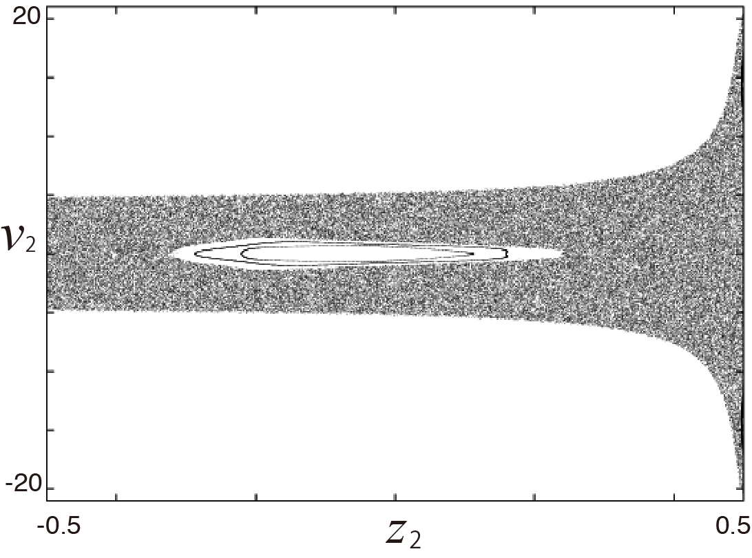
Figure 19: Poincaré map 1 for attractive interaction with $\varepsilon=5$.

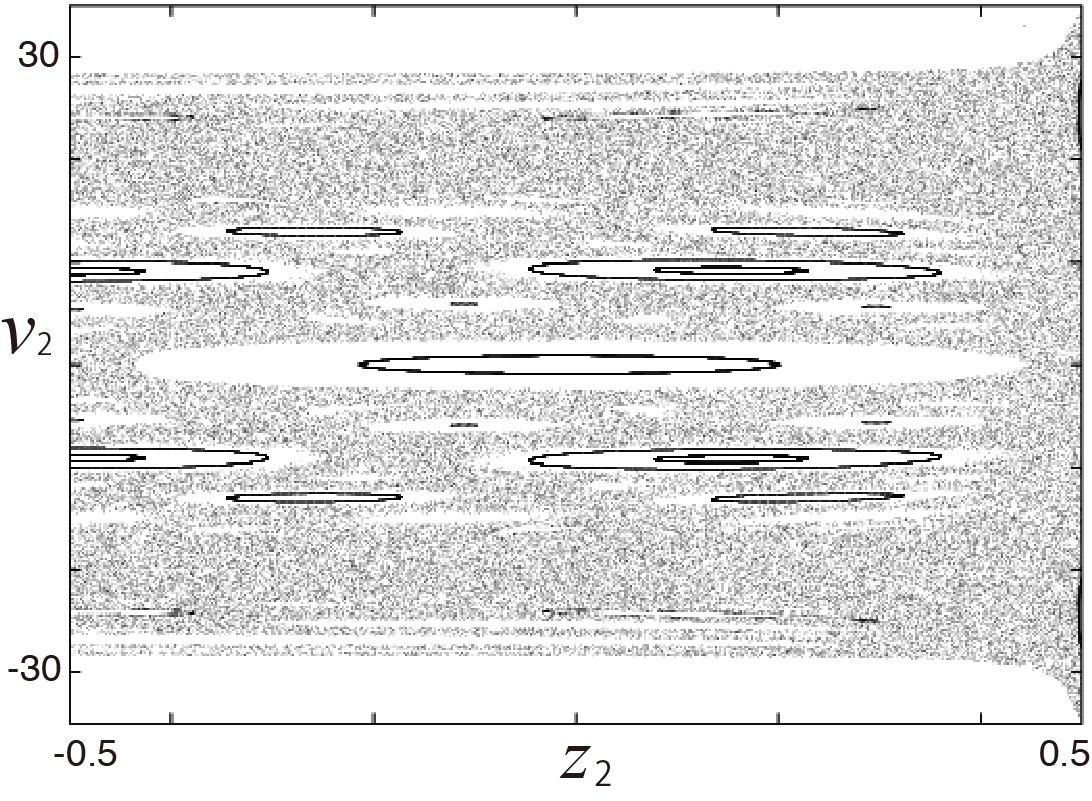
Figure 20: Poincaré map 1 for attractive interaction with $\varepsilon=200$.

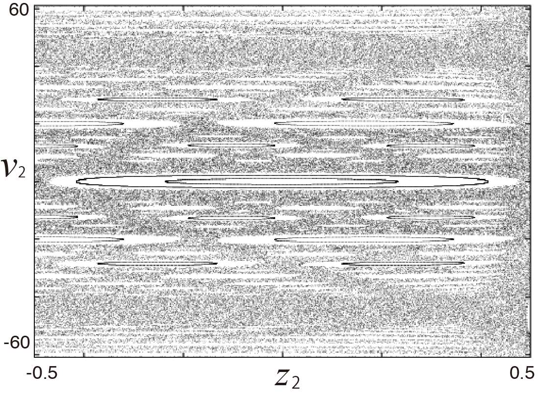
Figure 21: Poincaré map 1 for attractive interaction with $\varepsilon=1000$.

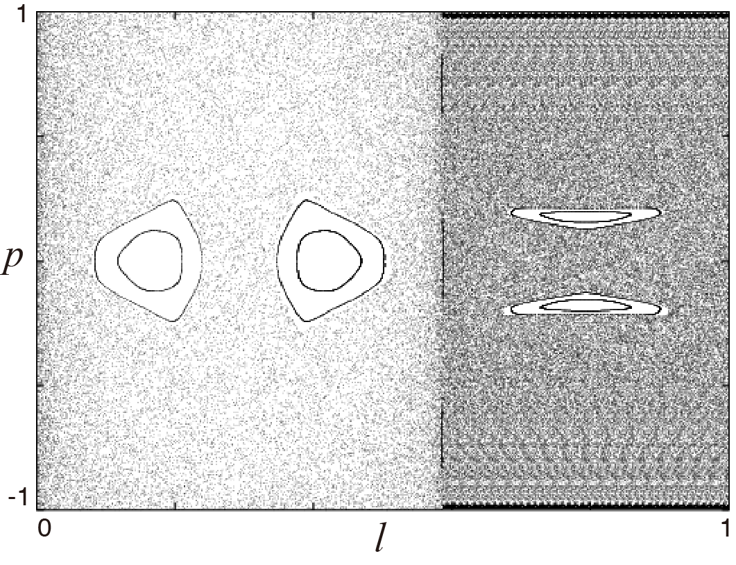
Figure 22: Poincaré map 2 for attractive interaction with $\varepsilon=5$.

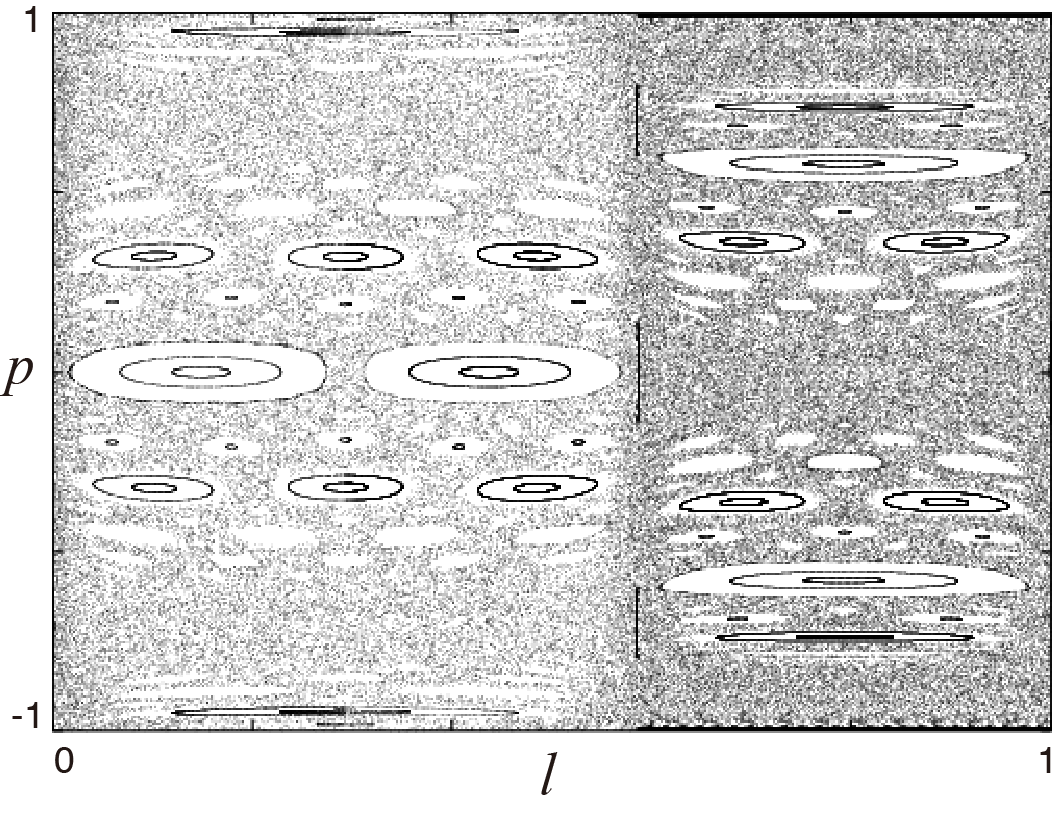
Figure 23: Poincaré map 2 for attractive interaction with $\varepsilon=200$.

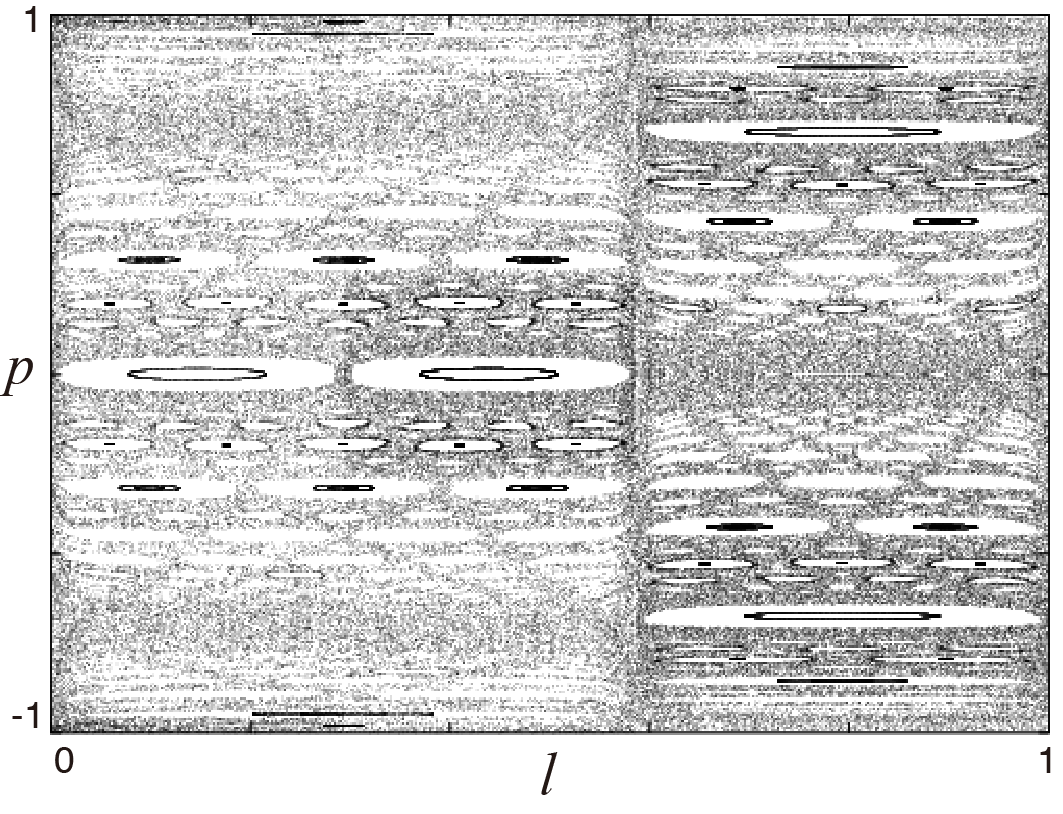
Figure 24: Poincaré map 2 for attractive interaction with $\varepsilon=1000$.

We calculate $\Gamma_{L}^{\prime}$ in Eq.(22) with $\xi=0.01$, which reflects the degree of chaotic irregularity. Numerical calculations of the trajectories are performed for time more than $1.5\times 10^{5}$. The results are shown in Fig.25, where we see that $\Gamma_{L}^{\prime}$ decreases with increase of $\varepsilon$ for $\varepsilon>0$. This is consistent with the fact that the dynamics of the particle becomes regular when $\varepsilon$ increases for $\varepsilon>0$.

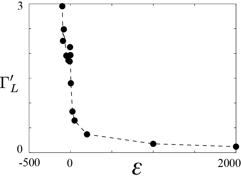
Figure 25: $\varepsilon-$dependence of $\Gamma_{L}^{\prime}$ in Eq.(22) for the attractive interaction. The broken line is a guide to the eyes.

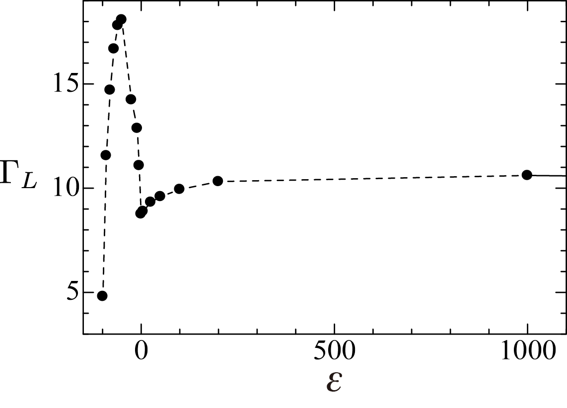
Figure 26: The same as Fig.25 except for MLE $\Gamma_{L}$ in Eq.(21).

On the other hand, $\Gamma_{L}$ in Eq.(21) increases with $\varepsilon$ as seen in Fig.26, where we take $\Delta t=0.01$. The increase of $\Gamma_{L}$ is due to the fact that the dynamics of the particle becomes faster with the increase of $\varepsilon$. $\Gamma_{L}$ does not reflect degree of chaotic irregularity of the classical system similarly to the case of the repulsive interaction.

We also calculate the ratio $R_{a}$ between two areas in Poincaré maps, the area of the largest irregular region and the area of total region reachable, in the same manner used for repulsive interaction. The $\varepsilon-$dependence of $R_{a}$ for Poincaré map 1 and 2 are shown in Figs.27 and 28, respectively. $R_{a}$ increases with $\varepsilon$ for $\varepsilon>500$, while the orbit becomes more regular when $\varepsilon$ increases as well as in the case of the repulsive interaction. Therefore $R_{a}$ is not a proper measure of irregularity also for the case of the attractive interaction in present system.

Figure 27: $\varepsilon-$dependence of the ratio $R_{a}$ between two areas in Poincaré map 1. The broken line is a guide to the eyes.

Figure 28: The same as Fig.27 except for Poincaré map 2.

IV summary and conclusion

We studied dynamics of two spinless particles confined in a quantum wire with repulsive or attractive Coulomb interaction. The system is reduced to a quasi-one-dimensional system with effective potential under the assumption that the transverse confinement is much stronger than the longitudinal one.

The Coulomb interaction induces irregular dynamics in classical mechanics. Examining Poincaré maps for the present system, we have found that the classical system exhibits mixed dynamics with coexisting KAM tori and chaotic regions. To see the signatures of quantum chaos in the corresponding quantum system we analyzed the distributions of the nearest neighbor level spacing (NNLS), which is fitted to the Brody distribution function characterized by the Brody parameter $\alpha$. The results indicate that they are intermediate between the Poisson and Wigner distributions, which is consistent with the mixed character of the classical dynamics.

The present classical system has a scaling property: Its dynamics is characterized by the rescaled energy parameter $\varepsilon=E/|\lambda|$, where $\lambda$ is the interaction strength parameter. Contrastingly, the quantum system has no such scaling property. However it has turned out that the distribution of NNLS in the quantum system has a scaling property similarly to the case of classical mechanics. The Brody parameter $\alpha$ depends almost only on the average value of $\varepsilon$ and is insensitive to the value of $\lambda$ itself.

In the classical system, we found that orbits are more regular for larger values of $\varepsilon$. The ordinary MLE $\Gamma_{L}$ is not suitable measure of chaotic irregularity for the present system, because they increase with $\varepsilon$ whereas the irregularity of the system decreases. We introduced a new MLE $\Gamma_{L}^{\prime}$, which represents a rate of the exponential divergence of two adjacent orbits (reference and displaced orbits) with respect to the length of the reference orbit, while the ordinary Lyapunov exponent describes the one with respect to time. The dependence of $\Gamma_{L}^{\prime}$ on $\varepsilon$ quantitatively shows the decrease of chaotic irregularity with increase of $\varepsilon$. Therefore, the $\Gamma_{L}^{\prime}$ is a suitable measure of chaotic irregularity of the present classical system rather than $\Gamma_{L}$. On the other hand in quantum system, the Brody parameter $\alpha$ decreases almost monotonously with increase of the average value of $\varepsilon$ in both cases of the repulsive and attractive interactions which indicates the distribution function of NNLS approaches to Poisson distribution with increase of $\varepsilon$. Consequently, we have shown closer correspondence between the classical chaos and quantum chaos in the present system.

We also showed that the area of the irregular region in Poincaré maps are not suitable measure of chaotic irregularity for the present system in contrast with other systems in which the area has been adopted as a measure of irregularity by several authors Win ; Ter ; Har .

- (1) S. E. Ulloa, and D. Pfannkuche, Superlattice Microstruct. 21, 21 (1997).
- (2) L. Meza-Montes, S. E. Ulloa, D. Pfannkuche, Physica E 1, 274 (1998).
- (3) K-H. Ahn and K. Richter, Ann. Phys. (Leipzig) 8, 1 (1999).
- (4) K-H. Ahn, K. Richter,and I-H Lee, Phys. Rev. Lett. 83, 4144 (1999).
- (5) M. Van Vessen, Jr., M. C. Santos, Bin Kang Cheng, and M. G. E. da Luz, Phys. Rev. E 64, 026201 (2001).
- (6) A. J. Fendrik, M. J. Sánchez, and P. I. Tamborenea, Phys. Rev. B 63, 115313 (2001).
- (7) P. S. Drouvelis, P. Schmelcher,and F. K. Diakonos, Phys. Rev. B 69, 035333 (2004).
- (8) E.P.S. Xavier, M.C. Santos, L.G.G.V. Dias da Silva, M.G.E. da Luz, and M.W. Beimsaand, Physica A 342, 377 (2004).
- (9) S. Sawada, A. Terai, and K. Nakamura, Chaos, Solitons and Fractals 40, 862 (2009).
- (10) E. Haller, H. Kppel, and L. S. Cederbaum, Phys. Rev. Lett. 52, 1665 (1984).
- (11) Th. Zimmermann, H.-D. Meyer, H. Kppel, and L. S. Cederbaum, Phys. Rev. A 33, 4334 (1986).
- (12) Y. H. Zeng, and R. A. Serota, Phys. Rev. B 50, 2492 (1994).
- (13) D. Wintgen, and H. Friedrich, Phys. Rev. A 35, 1464 (1987).
- (14) T. Terasaka, and T. Matsushita, Phys. Rev. A 32, 538 (1985).
- (15) A. Harada and H. Hasegawa, J. Phys. A Math. Gen. 16, L259-L263 (1983).