Double Spin Asymmetry of Electrons from Heavy Flavor Decays
in $p$$+$$p$ Collisions at $\sqrt{s}=200$ GeV

Abstract

We report on the first measurement of double-spin asymmetry, $A_{LL}$, of electrons from the decays of hadrons containing heavy flavor in longitudinally polarized $p$$+$$p$ collisions at $\sqrt{s}=200$ GeV for $p_{T}=$ 0.5 to 3.0 GeV/$c$. The asymmetry was measured at midrapidity ($|\eta|<0.35$) with the PHENIX detector at the Relativistic Heavy Ion Collider. The measured asymmetries are consistent with zero within the statistical errors. We obtained a constraint for the polarized gluon distribution in the proton of $|\Delta g/g(\log_{10}x=-1.6^{+0.5}_{-0.4},\mu=m_{T}^{c})|^{2}<0.033~{}(1\sigma$) based on a leading-order perturbative-quantum-chromodynamics model, using the measured asymmetry.

I Introduction

The measurement of the first moment of the proton’s spin-dependent structure function $g_{1}^{p}$ by the European Muon Collaboration (EMC) Ashman et al. (1988, 1989) revealed a discrepancy from the Ellis-Jaffe sum rule Ellis and Jaffe (1974); Kodaira (1980) and also the fact that the SU(3) flavor-singlet axial charge $g_{\rm{A}}^{(0)}$ was smaller than expected from the static and relativistic quark models D. Bass (1989). After these discoveries, experimental efforts Airapetian et al. (2007); Alexakhin et al. (2007a, b) focused on a detailed understanding of the spin structure of the proton. The proton spin $s_{z}/\hbar=1/2$ can be decomposed as $\frac{1}{2}=\frac{1}{2}\Delta\Sigma+\Delta G+L_{z}$ from conservation of angular momentum. The measurements precisely determined the total spin carried by quarks and anti-quarks, $\Delta\Sigma$, which is only about $30$% of the proton spin. The remaining proton spin can be attributed to the other components, the gluon spin contribution ($\Delta G$) and/or orbital angular momentum contributions ($L_{z}$). The total gluon polarization is given by

$$\Delta G(\mu)\equiv\int_{0}^{1}dx\Delta g(x,\mu),$$ (1)

where $x$ and $\mu$ represent Bjorken $x$ and factorization scale respectively. The challenge for the $\Delta G(\mu)$ determination is to precisely map the gluon polarization density $\Delta g(x,\mu)$ over a wide range of $x$.

The Relativistic Heavy Ion Collider (RHIC), which can accelerate polarized proton beams up to 255 GeV, is a unique and powerful facility to study the gluon polarization. One of the main goals of the RHIC physics program is to determine the gluon polarization through measurements of longitudinal double-spin asymmetries,

$$A_{LL}\equiv\frac{\sigma^{++}-\sigma^{+-}}{\sigma^{++}+\sigma^{+-}},$$ (2)

where $\sigma^{++}$ and $\sigma^{+-}$ denote the cross sections of a specific process in the polarized $p$$+$$p$ collisions with same and opposite helicities. Using $A_{LL}$, the polarized cross sections, $\sigma^{++}$ and $\sigma^{+-}$, can be represented as,

$$\sigma^{+\pm}=\sigma_{0}(1\pm A_{LL}),$$ (3)

where $\sigma_{0}$ is the unpolarized cross section of the process. $A_{LL}$ has been measured previously in several channels by PHENIX and STAR, including inclusive $\pi^{0}$ Adare et al. (2009a); Adare et al. (2007); Adler et al. (2006a); Adare et al. (2009b), $\eta$ Adare et al. (2011a), and jet Djawotho et al. ; Abelev et al. (2008); Adare et al. (2011b) production.

Using the measured asymmetries, as well as the world-data on polarized inclusive and semi-inclusive deep-inelastic scattering (DIS) Airapetian et al. (2007); Alexakhin et al. (2007a, b); Airapetian et al. (2005); Alekseev et al. (2008), a global analysis based on perturbative-quantum-chromodynamics (pQCD) calculation was performed at next-to-leading order (NLO) in the strong-coupling constant $\alpha_{S}$ de Florian et al. (2009). The resulting $\Delta g(x,\mu)$ from the best fit is too small to explain the proton spin in the Bjorken $x$ range of $0.05<x<0.2$ ($-1.3<\log_{10}x<-0.7$) without considering $L_{z}$, though a substantial gluon polarization is not ruled out yet due to the uncertainties. Also, due to the limited Bjorken $x$ coverage, there is a sizable uncertainty in Eq. 1 from the unexplored small $x$ region.

The polarized cross section of heavy flavor production on the partonic level is well studied with leading-order (LO) and NLO pQCD calculations Karliner and Robinett (1994); Bojak and Stratmann (2003); Bojak . The heavy quarks are produced dominantly by the gluon-gluon interaction at the partonic level Riedl et al. . Therefore, this channel has good sensitivity to the polarized gluon density. In addition, the large mass of the heavy quark ensures that pQCD techniques are applicable for calculations of the cross section. Therefore, the measurement of heavy flavor production in polarized proton collisions is a useful tool to study gluon polarization.

In $p$$+$$p$ collisions at $\sqrt{s}=200$ GeV, the heavy flavor production below $p_{T}\sim 5$ GeV/$c$ is dominated by charm quarks. The Bjorken $x$ region covered by this process at midrapidity is centered around $2m_{c}/\sqrt{s}\sim 1.4\times 10^{-2}$ where $m_{c}$ represents the charm quark mass. Hence, measurement of the spin dependent heavy flavor production is sensitive to the unexplored $x$ region, and complements other data on the total gluon polarization $\Delta G(\mu)$.

At PHENIX, hadrons containing heavy flavors are measured through their semi-leptonic decays to electrons and positrons (heavy flavor electrons) Adler et al. (2006b); Adare et al. (2011c). Therefore the double-spin asymmetry of the heavy flavor electrons is an important measurement for the gluon polarization study. In this paper, we report the first measurement of this asymmetry, and a resulting constraint on the gluon polarization with an LO pQCD calculation.

The organization of this paper is as follows: We introduce the PHENIX detector system used for the measurement in Sec. II. The method for the heavy flavor electron analysis is discussed in Sec. III and the results of the cross section and the spin asymmetry are shown in Sec. IV and Sec. V, respectively. From the asymmetry result, we estimate a constraint on the polarized gluon density, which is described in Sec. VI. For the sake of simplicity, we use the word “electron” to include both electron and positron throughout this paper, and distinguish by charge where necessary.

II Experimental Setup

This measurement is performed with the PHENIX detector positioned at one of collision points at RHIC. The RHIC accelerator comprises the blue ring circulating clockwise and the yellow ring circulating counter-clockwise. For this experiment, polarized bunches are stored and accelerated up to 100 GeV in each ring and collide with longitudinal polarizations of $\sim 57$% along the beams at the collision point with a collision energy of $\sqrt{s}=200$ GeV. The bunch polarizations are changed to parallel (beam-helicity $+$) or anti-parallel (beam-helicity $-$) along the beams alternately in the collisions to realize all 4 ($=2\times 2$) combinations of the crossing beam-helicities. Each time the accelerator is filled, the pattern of beam helicities in the bunches is changed, in order to confirm the absence of a pattern dependence of the measured spin asymmetry. See Sec. V for details.

A detailed description of the complete PHENIX detector system can be found elsewhere Adcox et al. (2003a, b, c); Aizawa et al. (2003); Aphecetche et al. (2003); Akikawa et al. (2003); Allen et al. (2003). The main detectors that are used in this analysis are beam-beam counters (BBC), zero degree calorimeters (ZDC), and two central arm spectrometers. The BBC provides the collision vertex information and the minimum bias (MB) trigger. The luminosity is determined by the number of MB triggers. Electrons are measured with the two central spectrometer arms which each cover a pseudorapidity range of $|\eta|<0.35$ and azimuthal angle $\Delta\phi=\pi/2$.

Figure 1 shows the beam view of the 2009 PHENIX central arms configuration, which comprises the central magnet (CM), drift chamber (DC), and pad chamber (PC) [for charged particle tracking], the ring-imaging Čerenkov detector (RICH) and hadron blind detector (HBD) Kazlov et al. (2004); Anderson et al. (2011) [for electron identification], and the electromagnetic calorimeter (EMCal) [for energy measurement]. Below we summarize the features of the detectors and the CM.

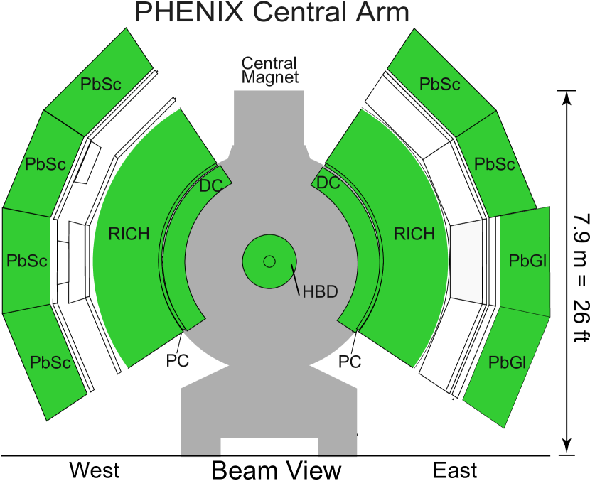
Figure 1: (color online) Beam view (at $z=0$) of the PHENIX central arm detectors in 2009. See text for details.

The BBCs are two identical counters positioned at $\pm 1.44$ m from the nominal interaction point along the beam direction and cover pseudorapidity of $3.1<|\eta|<3.9$. They measure the collision vertex along the beam axis by measuring the time difference between the two counters, and also provide the MB trigger defined by at least one hit on each side of the vertex. The position resolution for the vertex is $\sim 2.0$ cm in $p$$+$$p$ collision.

The ZDCs, which are located at $\pm 18.0$ m away from the nominal interaction point along the beam direction, detect neutral particles near the beam axis ($\theta<2.5$ mrad). Along with the BBCs, the trigger counts recorded by the ZDCs are used to determine the relative luminosity between crossings with different beam-helicities combinations. The ZDCs also serve for monitoring the orientation of the beam polarization in the PHENIX interaction region through the experiment.

The transverse momentum of a charged particle track is determined by its curvature in the magnetic field provided by the PHENIX CM system Adcox et al. (2003b). The CM is energized by two pairs of concentric coils and provides an axial magnetic field parallel to the beam direction. During this measurement, the two coils of the CM were operated in the canceling (“$+-$”) configuration. This configuration is essential for the background rejection of the heavy flavor electron measurement with the HBD as described later. In this configuration, the field is almost canceled out around the beam axis in the radial region $0<R<50$ cm, and has a peak value of $\sim 0.35$ T around $R\sim 100$ cm. The total field integral is $|\int B\times dl|=0.43$ Tm.

The DC and PC in the central arms measure charged particle trajectories in the azimuthal direction to determine the transverse momentum ($p_{T}$) of each particle. By combining the polar angle measured by the PC and the vertex information along the beam axis from the BBC with $p_{T}$, the total momentum $p$ is determined. The DC is positioned between $202$ cm and $246$ cm in radial distance from the collision point for both the west and east arms and the PC is $247$-$252$ cm.

The RICH is a threshold-type gas $\check{\rm{C}}$erenkov counter and the primary detector used to identify electrons in PHENIX. It is located in the radial region of $2.5$-$4.1$ m. The RICH has a $\check{\rm{C}}$erenkov threshold of $\gamma=35$, which corresponds to $p=20$ MeV/$c$ for electrons and $p=4.9$ GeV/$c$ for charged pions.

The EMCal comprises four rectangular sectors in each arm. The six sectors based on lead-scintillator calorimetry and the two (lowest sectors on the east arm) based on lead-glass calorimetry are positioned at radial distances from the collision point of $\sim 5.1$ m and $\sim 5.4$ m, respectively.

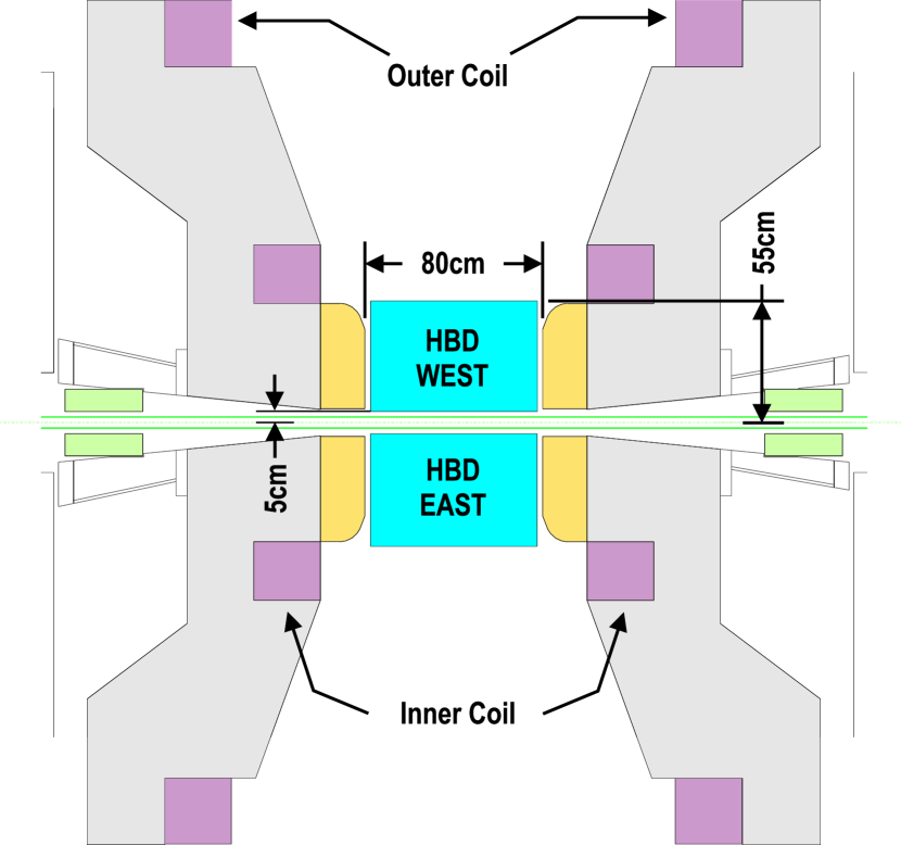
(a) HBD from top view.

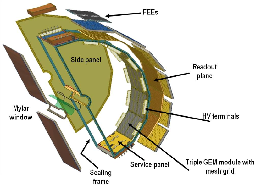
(b) HBD exploded view.

Figure 2: (color online) (a) Top view of the HBD showing the location of the HBD in the central magnet. (b) Exploded view of one half HBD arm. CF₄ gas is filled in the volume as the $\check{\rm{C}}$erenkov light radiator.

A challenging issue for the heavy flavor electron measurement is to reject the dominant background of electron pairs from $\gamma$ conversions and Dalitz decays of $\pi^{0}$ and $\eta$ mesons, which are mediated by virtual photons. These electrons are called “photonic electrons”, while all the other electrons are called “nonphotonic electrons”. Most nonphotonic electrons are from heavy flavor decays, however, electrons from $K_{e3}$ decays ($K\rightarrow e\nu\pi$) and the dielectron decays of light vector mesons are also nonphotonic Adler et al. (2006b). The HBD aims to considerably reduce the photonic electron pairs utilizing distinctive feature of the $e^{+}e^{-}$ pairs, namely their small opening angles.

The HBD is a position-sensitive $\check{\rm{C}}$erenkov detector operated with pure CF₄ gas as a radiator. It covers pseudorapidity $|\eta|<0.45$ and $2\times 3\pi/4$ in azimuth. The coverage is larger than the acceptance of the other detectors in the central arm in order to detect photonic electron pairs with only one track reconstructed in the central arm and the other outside of the central arm acceptance. Figure 2 shows the top view and exploded view of the HBD. The HBD has a $50$ cm long radiator directly coupled in a windowless configuration to a readout element consisting of a triple Gas Electron Multiplier (GEM) stack, with a CsI photocathode evaporated on the top surface of the GEM facing the collision point and pad readout at the exterior of the stack. The readout element in each HBD arm is divided into five sectors. The expected number of photoelectrons for an electron track is about 20, which is consistent with the measured number. Since the HBD is placed close to the collision point, the material thickness is small in order to minimize conversions. The total thickness to pass through the HBD is $0.024X_{0}$ and the thickness before the GEM pads is $0.007X_{0}$.

The $\check{\rm{C}}$erenkov light generated by electrons is directly collected on a photosensitive cathode plane, forming an almost circular blob image. The readout pad plane comprises hexagonal pads with an area of $6.2$ cm² (hexagon side length $a=1.55$ cm) which is comparable to, but smaller than, the blob size which has a maximum area of $9.9$ cm².

The HBD is located in a field free region that preserves the original direction of the $e^{+}e^{-}$ pair. The $\check{\rm{C}}$erenkov blobs created by electron pairs with a small opening angle overlap, and therefore generate a signal in the HBD with twice the amplitude of a single electron. Electrons originating from $\pi^{0}$ and $\eta$ Dalitz decays and $\gamma$ conversions can largely be eliminated by rejecting tracks which correspond to large signals in the HBD.

III Heavy Flavor Electron Analysis

With the improved signal purity from the HBD, the double helicity asymmetry of the heavy flavor electrons was measured. In this section, we explain how the heavy flavor electron analysis and the purification of the heavy flavor electron sample using the HBD was performed.

III.1 Data Set

The data used here were recorded by PHENIX during 2009. The data set was selected by a level-1 electron trigger in coincidence with the MB trigger. The electron trigger required a minimum energy deposit of $0.6$ GeV in a $2\times 2$ tile of towers in EMCal, $\check{\rm{C}}$erenkov light detection in the RICH, and acceptance matching of these two hits. After a vertex cut of $|z_{{\rm vtx}}|<20$ cm and data quality cuts, an equivalent of $1.4\times 10^{11}$ MB events, corresponding to $6.1$ pb^-1, sampled by the electron trigger were analyzed.

III.2 Electron Selection

Electrons are reconstructed using the detectors in the PHENIX central arm described above. Several useful variables for the electron selection which were used in the previous electron analysis in 2006 Adare et al. (2011c) are also used in this analysis. In addition to the conventional parameters, we introduced a new value, $q_{\rm{clus}}$, for the HBD analysis.

hbdcharge: $q_{\rm{clus}}$

Total charge of the associated HBD cluster calibrated in units of the number of photoelectrons (p.e.).

The electron selection cuts (eID-cut) are:

1. 4.0$\sigma$ matching between track and EMCal cluster

2. # of hit tubes in RICH around track $\geq 2$

3. 3.5$\sigma$ matching between track and HBD cluster

4. shower profile cut on EMCal

5. $0.57<E/p<1.37$ ($0.5$ GeV/$c$ $<p_{T}<1.0$ GeV/$c$)

6. $0.60<E/p<1.32$ ($1.0$ GeV/$c$ $<p_{T}<1.5$ GeV/$c$)

7. $0.64<E/p<1.28$ ($1.5$ GeV/$c$ $<p_{T}<5.0$ GeV/$c$)

8. # of hit pads in HBD cluster $\geq 2$

9. $q_{\rm{clus}}>8.0$ p.e.

10. ($q_{\rm{clus}}>4.0$ p.e. for one low-gain HBD sector)

These cuts require hits in the HBD, RICH, and EMCal that are associated with projections of the track onto these detectors. The shower profile in the EMCal is required to match the profile expected of an electromagnetic shower. For electrons, the energy deposit on EMCal, $E$, and the magnitude of the reconstructed momentum on DC and PC, $p$, should match due to their small mass. Therefore the ratio, $E/p$, was required to be close to 1. Since the energy resolution of the EMCal depends on the momentum of the electron, the cut boundaries were changed in different momentum range. Charged particles traversing the CF₄ volume in the HBD produce also scintillation light, which has no directivity and creates hits with small charge in random locations in the GEM pads. To remove HBD background hits by the scintillation light, a minimum charge and a minimum cluster size were required for the HBD hit clusters. During this measurement, the efficiency for the $\check{\rm{C}}$erenkov light in one HBD sector was low compared with other sectors. Hence we apply a different charge cut to that HBD sector for the electron selection.

The $E/p$ distribution for tracks selected with these cuts is shown in Fig. 3. The clear peak around $E/p=1$ corresponds to electrons and the spread of events around the peak consists mainly of electrons from $K_{e3}$ decays and misidentified hadrons. As the figure shows, the fraction of these background tracks in the reconstructed electron sample after applying eID-Cut including the $E/p$ cut was small. The fractions of the $K_{e3}$ decays and the misidentified hadrons are described in Sec. III.4 and Sec. III.5.

As mentioned in Sec. II, we remove the photonic electrons and purify the heavy flavor electrons on the basis of the associated HBD cluster charge. The nonphotonic electron cuts (npe-Cut) are:

1. $8.0<q_{\rm{clus}}<28.0$ p.e.

2. ($4.0<q_{\rm{clus}}<17.0$ p.e. for 1 low-gain HBD sector)

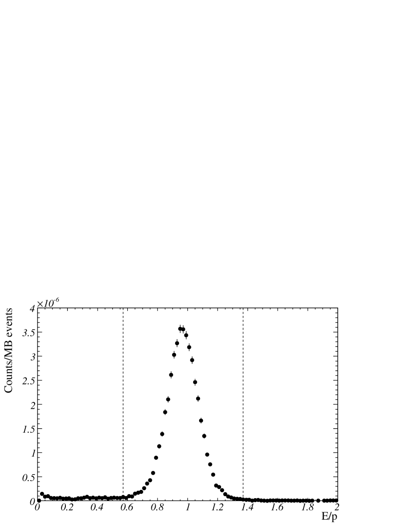
Figure 3: $E/p$ distributions for $0.5$ GeV/$c$ $<p_{T}<1.0$ GeV/$c$ reconstructed charged tracks with the eID-Cut other than the $E/p$ cut. Criteria of the $E/p$ cut for the momentum region are shown by dashed lines in the plot.

III.3 Yield estimation of heavy flavor electrons with HBD

We categorize the HBD hit clusters into three types according to the source of the cluster. A cluster created by a single blob of $\rm{\check{C}}$erenkov light from a nonphotonic electron as shown in Fig. 4(a) is defined as a single cluster. On the other hand, a cluster created by merging blobs of $\rm{\check{C}}$erenkov light from a track pair of photonic electrons as shown in Fig. 4(b) is defined as a merging cluster. However, a portion of the photonic electrons which have a large enough opening angle such that the two cluster do not merge (typically $\lower 2.15277pt\hbox{$\;\buildrel>\over{\sim}\;$}0.1$ rad) creates two separated single clusters as shown in Fig. 4(c). Therefore the single clusters are created by both of the nonphotonic electron and the photonic electron with a large opening angle.

We also define another type of cluster created by scintillation light, which we call a scintillation cluster. Scintillation hits which accidentally have large hit charges and have neighboring hits can constitute clusters. Photonic electrons from $\gamma$ conversions after the HBD GEM pads do not create $\rm{\check{C}}$erenkov light in the HBD gas volume. Hence they basically do not have associated clusters in the HBD and they are rejected by the HBD hit requirement in the eID-Cut. However, a portion of these are accidentally associated with scintillation clusters and satisfy the eID-Cut and so also survive in the reconstructed electron sample.

In Sec. III.3.1, we estimated yields of these clusters from the distribution shape of the HBD cluster charge. We also estimated the small component of single clusters generated from photonic electrons which have the large opening angles as described in Sec. III.3.2. Then we determined the nonphotonic electron yield. Subtracting additional background electrons from $K_{e3}$ decays and $e^{+}e^{-}$ decays of light vector mesons, we obtain the heavy flavor electron yield as described in Sec. III.3.3.

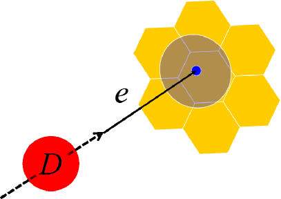
(a) Non-photonic electrons.

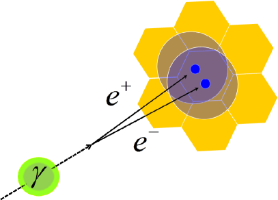
(b) Photonic electrons (merging cluster).

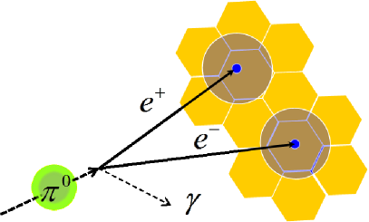
(c) Photonic electrons (separated clusters).

Figure 4: (color online) Responses of the HBD for (a) nonphotonic electrons and (b,c) photonic electrons. (b) Most of the photonic electron pair create merging clusters. (c) However, the photonic electrons with large opening angles create separated clusters.

III.3.1 Yield estimation of single clusters

All clusters associated with the reconstructed electrons can be classified into the above three types. The yield of the electrons associated with the single clusters must be evaluated to estimate the yield of the heavy flavor electrons. The shapes of the $q_{\rm{clus}}$ distributions for the three cluster types are quite different since merging clusters have basically double the charge of single clusters and the charge of scintillation clusters is considerably smaller than the charge of the single cluster. Using the difference in the shapes, we estimate yields of these clusters as follows.

The probability distributions of $q_{\rm{clus}}$ for single and merging clusters were estimated by using low-mass unlike-sign electron pairs reconstructed with only the eID-Cut, which is dominated by photonic electron pairs. We defined the unlike-sign electron pairs whose two electrons were associated with two different HBD clusters as separated electron pairs and the pairs whose two electrons were associated to the same HBD cluster as merging electron pairs. The probability distribution of $q_{\rm{clus}}$ for the single clusters were estimated by the $q_{\rm{clus}}$ distribution of the separated electron pairs and the probability distribution of $q_{\rm{clus}}$ for the merging clusters were estimated by the $q_{\rm{clus}}$ distribution of the merging electron pairs. The reconstruction of the electron pairs creates a small bias on the shapes of the $q_{\rm{clus}}$ distributions. Corrections for this bias are estimated by simulation and applied to the distributions. The probability distributions are denoted as $f_{\rm{c}}^{\rm{s}}(q_{\rm{clus}})$ for the single clusters and $f_{\rm{c}}^{\rm{m}}(q_{\rm{clus}})$ for the merging clusters. The probability distribution of $q_{\rm{clus}}$ for the scintillation clusters is also estimated by the distribution of the hadron tracks reconstructed by the DC/PC tracking and the RICH veto and denoted as $f_{\rm{c}}^{\rm{sci}}(q_{\rm{clus}})$.

The variables used in the hbdcharge analysis are:

$f_{\rm{c}}^{\rm{s}}$

Probability distribution of $q_{\rm{clus}}$ for the single clusters

$f_{\rm{c}}^{\rm{m}}$

Probability distribution of $q_{\rm{clus}}$ for the merging clusters

$f_{\rm{c}}^{\rm{sci}}$

Probability distribution of $q_{\rm{clus}}$ for the scintillation clusters

$n_{\rm{s}}$

Number of single clusters after applying eID-Cut.

$n_{\rm{m}}$

Number of merging clusters after applying eID-Cut.

$n_{\rm{sci}}$

Number of scintillation clusters after applying eID-Cut.

$\tilde{n}_{\rm{s}}$

Number of single clusters after applying eID-Cut and npe-Cut.

$\tilde{n}_{\rm{m}}$

Number of merging clusters after applying eID-Cut and npe-Cut.

$\tilde{n}_{\rm{sci}}$

Number of scintillation clusters after applying eID-Cut and npe-Cut.

The $q_{\rm{clus}}$ distribution of the reconstructed electrons found by applying eID-Cut is fitted with a superposition of the three probability distributions

$$\begin{array}[]{cc}n_{\rm{s}}\times f_{\rm{c}}^{\rm{s}}(q_{\rm{clus}})&+\\ n_{\rm{m}}\times f_{\rm{c}}^{\rm{m}}(q_{\rm{clus}})&+\\ n_{\rm{sci}}\times f_{\rm{c}}^{\rm{sci}}(q_{\rm{clus}}),&\end{array}$$ (4)

where $n_{\rm{s}}$, $n_{\rm{m}}$ and $n_{\rm{sci}}$ are fitting parameters that represent the numbers of the reconstructed electrons associating to single clusters, merging clusters and scintillation clusters after applying eID-Cut respectively. The fraction of nonphotonic electrons and photonic electrons are different in different $p_{T}$ region of the reconstructed electron sample. Therefore the fitting was performed for each $p_{T}$ region and $n_{\rm{s}}(p_{T})$, $n_{\rm{m}}(p_{T})$ and $n_{\rm{sci}}(p_{T})$ for each $p_{T}$ region were determined. In the fitting, the distribution functions, $f_{\rm{c}}^{\rm{s}}(q_{\rm{clus}})$, $f_{\rm{c}}^{\rm{m}}(q_{\rm{clus}})$, and $f_{\rm{c}}^{\rm{sci}}(q_{\rm{clus}})$, are assumed to be $p_{T}$ independent because the velocity of electrons in $p_{T}$ region of interest is close enough to the speed of light in vacuum such that the yield of $\rm{\check{C}}$erenkov light from the electron is nearly independent of $p_{T}$. We also compared the shapes of the distributions in different $p_{T}$ regions to confirm that the effect from the track curvature is small enough to be ignored even at $p_{T}\sim 0.5$ GeV/$c$. On the other hand, $f_{\rm{c}}^{\rm{s}}(q_{\rm{clus}})$, $f_{\rm{c}}^{\rm{m}}(q_{\rm{clus}})$ and $f_{\rm{c}}^{\rm{sci}}(q_{\rm{clus}})$ for different HBD sectors vary slightly. Considering this difference, the fitting is performed for each sector individually.

The $q_{\rm{clus}}$ distribution for the reconstructed electrons with transverse momentum $p_{T}$ ranging from $0.75$ GeV/$c$ to $1.00$ GeV/$c$ and the fitting result are shown in Fig. 5 for one HBD sector. The charge distribution of the reconstructed electrons is well reproduced by the superposition of the three individual components.

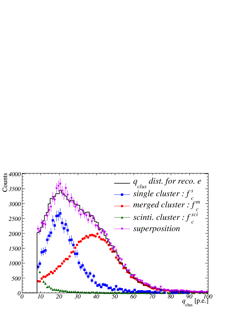
Figure 5: (color online). Charge distribution of HBD clusters associated with reconstructed electrons with a transverse momentum ranging from $0.75$ GeV/$c$ to $1.00$ GeV/$c$ (solid black line), and the charge distribution for each component, i.e., single clusters ($n_{\rm{s}}f_{\rm{c}}^{\rm{s}}$, blue circles), merging clusters ($n_{\rm{m}}f_{\rm{c}}^{\rm{m}}$, red squares), and scintillation clusters ($n_{\rm{sci}}f_{\rm{c}}^{\rm{sci}}$, green triangles). The superposition of these components is also shown (purple inverted triangles).

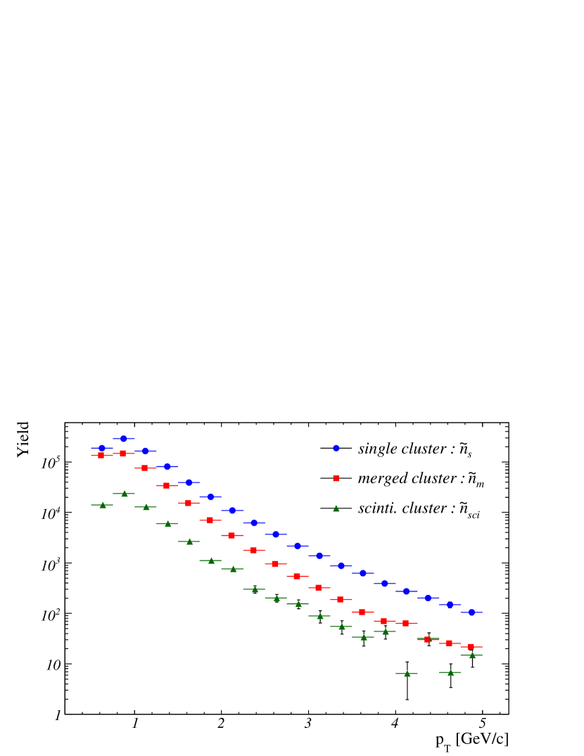
Figure 6: (color online). Yield spectra of HBD clusters after applying eID-Cut and npe-Cut estimated from the HBD cluster charge fitting. The plot shows the spectrum for the single clusters ($\tilde{n}_{\rm{s}}$, blue circle), the spectrum for the merging clusters ($\tilde{n}_{\rm{m}}$, red square) and the spectrum for the scintillation clusters ($\tilde{n}_{\rm{sci}}$, green triangle). The error bars represent fitting uncertainties.

The total number of reconstructed electrons after applying both of eID-Cut and npe-Cut for the three cluster types, which are represented as $\tilde{n}_{\rm{s}}$, $\tilde{n}_{\rm{m}}$ and $\tilde{n}_{\rm{sci}}$, are calculated by applying the npe-Cut efficiencies of $\int_{q_{{\rm min}}}^{q_{{\rm max}}}dqf^{\rm{s}}_{\rm{c}}(q)$, $\int_{q_{{\rm min}}}^{q_{{\rm max}}}dqf^{\rm{m}}_{\rm{c}}(q)$ and $\int_{q_{{\rm min}}}^{q_{{\rm max}}}dqf^{\rm{sci}}_{\rm{c}}(q)$ to the fit results, $n_{\rm{s}}$, $n_{\rm{m}}$ and $n_{\rm{sci}}$, respectively. In the integrals, $q_{{\rm min}}$ and $q_{{\rm max}}$ represent the HBD charge boundaries in the npe-Cut of $8$ p.e. and $28$ p.e. ($4$ p.e. and $17$ p.e. for the low-gain sector). The variables, $\tilde{n}$, are also summarized above. Figure 6 shows the yield spectra from the calculation as functions of $p_{T}$.

III.3.2 Yield estimation of separated photonic electrons

The estimated $\tilde{n}_{\rm{s}}$ is the sum of nonphotonic electrons and photonic electrons which create the separated clusters in the HBD. In the following description, we denote the photonic electrons which create merging clusters as merging photonic electrons (MPE) and those which create separated single clusters as separated photonic electrons (SPE). In this section, the number of SPE is estimated to obtain the yield of the nonphotonic electrons.

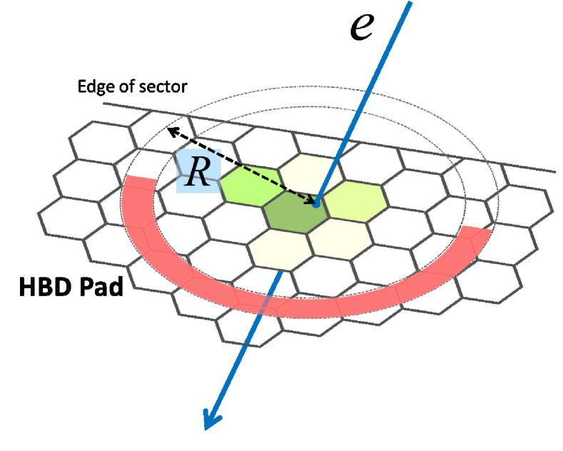
Figure 7: (color online). A half of an annular region around the reconstructed electron track on the HBD for the definition of hbdringcharge. The inner and outer radii of the annular region are 7.0 cm and 8.0 cm respectively. The direction of the half region is determined as the opposite side to the edge of the HBD sector to avoid inefficiency around the edge.

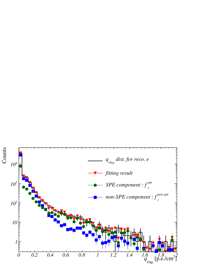
Figure 8: (color online). HBD charge distribution in the annular region for the reconstructed electrons with a transverse momentum ranging from 0.75 GeV/$c$ to 1.00 GeV/$c$ (solid black line), and the fitting result of the charge distribution for electrons with correlated charges ($n_{\rm{spe}}f_{\rm{r}}^{\rm{spe}}$, green circle) and without correlated charges ($n_{\rm{non\mathchar 45\relax spe}}f_{\rm{r}}^{\rm{non\mathchar 45\relax spe}}$, blue square), and the superposition of the fitting results (red inverted triangle).

In the case where a reconstructed electron track is identified as an SPE, the partner electron generates an additional signal in the HBD, as illustrated in Fig. 4(c). This property is utilized to estimate the number of SPE. For this estimation, we defined a new value, $q_{\rm{ring}}$, as

hbdringcharge: $q_{\rm{ring}}$

The total charge in the HBD pads centered on a half of an annular region with an inner radius of $7.0$ cm and an outer radius of $8.0$ cm around the track projection of HBD as shown in Fig. 7. To avoid inefficient regions around the edges of the HBD sectors, we use one half of an annular region oriented away from the nearest sector edge (see Fig. 7). The $q_{\rm{ring}}$ value is normalized by the area of the half of the annular region in the definition.

The choice of 7.0 cm to 8.0 cm is determined by three factors: (1) the distribution of distance between separated clusters of SPE has a maximum around 7.0 cm, (2) few HBD clusters have radii larger than 7.0 cm, and (3) larger area includes more scintillation background and decreases the signal to background ratio. Whereas the $q_{\rm{ring}}$ distributions for the nonphotonic electrons and MPE comprise signals only from scintillation light, the distributions for SPE include the correlated signals around the tracks in addition to scintillation light.

The variables used in the hbdringcharge analysis are:

$f_{\rm{r}}^{\rm{spe}}$

Probability distribution of $q_{\rm{ring}}$ for SPE

$f_{\rm{r}}^{\rm{non\mathchar 45\relax spe}}$

Probability distribution of $q_{\rm{ring}}$ for nonphotonic electrons and MPE

$n_{\rm{spe}}$

Number of SPE after applying the eID-Cut and npe-Cut.

$n_{\rm{non\mathchar 45\relax spe}}$

Number of electrons other than SPE after applying the eID-Cut and npe-Cut.

The $f_{\rm{r}}^{\rm{spe}}(q_{\rm{ring}})$ for SPE and the $f_{\rm{r}}^{\rm{non\mathchar 45\relax spe}}(q_{\rm{ring}})$ for nonphotonic electrons and MPE can be estimated by hadron tracks and electron tracks with large $q_{\rm{clus}}$ values, which consist almost entirely of MPE. Because hadrons and MPE clusters do not create any correlated signals around their tracks, the $q_{\rm{ring}}$ distributions of the tracks are created by only the scintillation light.

The $f_{\rm{r}}^{\rm{spe}}(q_{\rm{ring}})$ was estimated by using simulations. The dominant photonic electrons come from the Dalitz decays of $\pi^{0}$ and $\eta$ and $\gamma$ from their decays which convert in materials. We simulated the detector responses for the Dalitz decay and the $\gamma$ conversion events of the neutral mesons by a geant3 simulation GEA (1994) configured for the PHENIX detector system. The $\pi^{0}$ and $\eta$ spectra were parametrized in the simulation by $m_{T}$-scaled Tsallis distributions Adare et al. (2011d), together with their known branching ratios to Dalitz decays and $\gamma$ decays. In order to include contributions from scintillation light, $f_{\rm{r}}^{\rm{non\mathchar 45\relax spe}}(q_{\rm{ring}})$, which is identical to the $q_{\rm{ring}}$ distribution from only the scintillation light, was convoluted to the result to obtain $f_{\rm{r}}^{\rm{spe}}(q_{\rm{ring}})$.

The $q_{\rm{ring}}$ distribution for the reconstructed electrons selected by applying eID-Cut and npe-Cut was fitted with the superposition of the $q_{\rm{ring}}$ distributions, $f_{\rm{r}}^{\rm{spe}}(q_{\rm{ring}})$ and $f_{\rm{r}}^{\rm{non\mathchar 45\relax spe}}(q_{\rm{ring}})$, as

$$n_{\rm{spe}}\times f_{\rm{r}}^{\rm{spe}}(q_{\rm{ring}})+n_{\rm{non\mathchar 45\relax spe}}\times f_{\rm{r}}^{\rm{non\mathchar 45\relax spe}}(q_{\rm{ring}}),$$ (5)

where $n_{\rm{spe}}$ and $n_{\rm{non\mathchar 45\relax spe}}$ are fitting parameters and represent the numbers of SPE and other electrons in the $q_{\rm{ring}}$ distribution, respectively, as summarized above. Similar to the $q_{\rm{clus}}$ distribution, the fitting for the $q_{\rm{ring}}$ distribution was also performed for each electron $p_{T}$ region and each HBD sector. Figure 8 shows a fitting result in one HBD sector in the electron $p_{T}$ region from $0.75$ GeV/$c$ to $1.00$ GeV/$c$.

III.3.3 Yield estimation of heavy flavor electrons

Using the above fitting results of $\tilde{n}_{\rm{s}}$ and $n_{\rm{spe}}$, the yield of nonphotonic electrons, $N^{\rm{npe}}$ was estimated with the formula

$$N^{\rm{npe}}(p_{T}) = \tilde{n}_{\rm{s}}(p_{T})-n_{\rm{spe}}(p_{T}).$$ (6)

The remaining background for the heavy flavor electrons in the nonphotonic electron sample comes from $K_{e3}$ decays and $e^{+}e^{-}$ decays of light vector mesons, namely $\rho$, $\omega$, and $\phi$. Electrons from the Drell-Yan process also contribute to the background, however the contribution is known to be less than 0.5% of total heavy flavor electrons in this $p_{T}$ range and can be ignored. We determined the yield of the heavy flavor electrons from $N^{\rm{npe}}$ by subtracting the components of the $K_{e3}$ electrons, which are estimated by simulation using a measured $K$ cross section Adare et al. (2011d), and the electrons from light vector mesons, which are already estimated in previously published result Adler et al. (2006b), as

$$N^{{\rm{HFe}}}(p_{T})=N^{\rm{npe}}(p_{T})-N^{Ke3}(p_{T})-N^{\rm{LVM}}(p_{T}),$$ (7)

where $N^{Ke3}(p_{T})$ and $N^{\rm{LVM}}(p_{T})$ represent the electrons from the $K_{e3}$ decays and the light vector meson decays respectively.

III.4 Systematic Uncertainty

Table 1: Relative systematic uncertainties given on the heavy flavor electron yield.

source	uncertainty	$p_{T}$ range (GeV/$c$)
hbdringcharge fitting	$16\%$	( $0.50<p_{T}<0.75$ )
	$6\%\sim 4\%$	( $0.75<p_{T}<1.75$ )
	$2\%$	( $1.75<p_{T}$ )
hbdcharge fitting	$2\%$	( $0.50<p_{T}<0.75$ )
	$<1\%$	( $0.75<p_{T}$ )
$K_{e3}$	$4\%$	( $0.50<p_{T}<0.75$ )
	$<1\%$	( $0.75<p_{T}$ )
hadron misID	$4\%$	( $0.50<p_{T}<0.75$ )
	$<1\%$	( $0.75<p_{T}$ )

The systematic uncertainties for the heavy flavor electron yield come from the fits for the $q_{\rm{clus}}$ distribution and the $q_{\rm{ring}}$ distribution, and from estimations of $K_{e3}$ contribution and misidentified hadrons.

The most significant source in these contributions is the fitting uncertainty for the $q_{\rm{ring}}$ distribution. We varied the radius of the annular region to an inner radius of $6.0$ cm and an outer radius of $7.0$ cm and also to $8.0$ cm and $9.0$ cm from the default radii of $7.0$ cm and $8.0$ cm. The uncertainty from the fitting was set to the amount of variation in $n_{\rm{spe}}$ after these changes. The estimated uncertainties decrease from about 16% of the heavy flavor electron yield in the momentum range of $0.50<p_{T}<1.00$ GeV/$c$ to about 2% above 1.75 GeV/$c$.

The fitting uncertainty for the $q_{\rm{clus}}$ distribution comes from the estimation of the bias in the charge distribution shape due to the electron pair reconstruction. The systematic uncertainty from this effect is estimated to be less than 2% by simulation.

In the low momentum region, $0.50<p_{T}<1.00$ GeV/$c$, uncertainties from the $K_{e3}$ contribution and the hadron misreconstruction are significant. The uncertainty from the $K_{e3}$ contribution comes almost entirely from the uncertainty on the $K$ cross section used in the $K_{e3}$ simulation. This uncertainty amounts to about 4% of the total heavy flavor electron yield in the low momentum region and decreases to less than 1% for $p_{T}>0.75$ GeV/$c$. We also estimated the upper limits of the hadron contamination due to misreconstructions employing a hadron-enhanced event set. As a result, we determined the upper limits as 4% of the total heavy flavor electron yield in the low momentum region which decreases to less than 1% over 1.5 GeV/$c$. The upper limits are assigned as the systematic uncertainties from hadron misreconstructions. Table 1 summarizes the systematic uncertainties on the heavy flavor electron yield.

III.5 Results of Heavy Flavor Electron Yield and Signal Purity

From Eq. 6 and Eq. 7 and the discussion in Sec. III.4, the heavy flavor electron yield spectrum with the systematic uncertainties was determined. The spectrum is shown in Fig. 9. We also show the yield of inclusive reconstructed electrons after applying the eID-Cut and npe-Cut and the estimated $K_{e3}$ contribution. The electrons from $e^{+}e^{-}$ decays of the light vector mesons are not shown in Fig. 9, but they are less than 5% of the heavy flavor electron yield in this $p_{T}$ range.

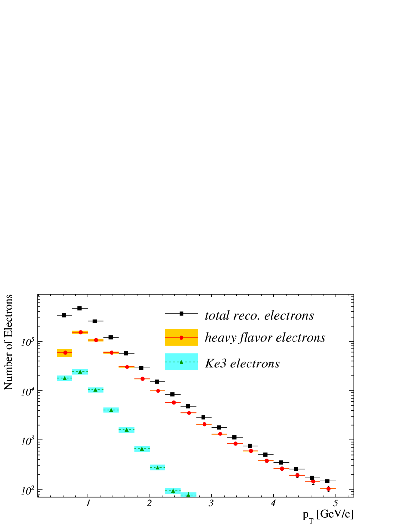
Figure 9: (color online). Heavy flavor electron yield spectrum. The black square points represent the total number of the reconstructed electrons after applying the eID-Cut and npe-Cut. The red circle points represent the estimated yield of the heavy flavor electrons. The yellow bands represent the systematic uncertainties for the heavy flavor electron yield. The green triangle points with dashed lines represent the estimated $K_{e3}$ contribution with systematic uncertainties shown by light-blue bands.

The ratio of the nonphotonic electron yield to the photonic electron yield in this measurement,

$$R(p_{T})\equiv\frac{N^{\rm{npe}}(p_{T})}{N^{\rm{reco}}_{e}(p_{T})-N^{\rm{npe}}(p_{T})}$$ (8)

where $N^{\rm{reco}}_{e}$ denotes the total number of reconstructed electrons after applying the eID-Cut and npe-Cut, is shown in the top panel of Fig. 10. In Eq. 8, we assumed the fraction of misidentified hadrons in the reconstructed electrons after the cuts is negligible as shown in Fig. 3, and so the number of photonic electrons can be represented as $N^{\rm{reco}}_{e}(p_{T})-N^{\rm{npe}}(p_{T})$. The same ratio from a previous measurement Adler et al. (2006b) is also shown in the figure. The previous measurement employed two other methods for the background estimation, namely a cocktail method and a converter method. In the cocktail method, a sum of electron spectra from various background sources was calculated using a Monte Carlo hadron decay generated. This sum was subtracted from the inclusive electron sample to isolate the heavy flavor contribution. With the converter method, a photon converter around the beam pipe was introduced to increase the photon conversion probability by a well-defined amount, and thus allow determination of the photonic background. The nonphotonic to photonic electron ratio is improved by a factor of about 2 or more in $p_{T}>1.0$ GeV/$c$ compared with the previously measured result due to the rejection of photonic electrons by the HBD.

The signal purity is defined as the ratio of the yield of the heavy flavor electrons to the reconstructed electrons after applying the eID-Cut and npe-Cut,

$$D(p_{T})\equiv\frac{N^{\rm{HFe}}(p_{T})}{N^{\rm{reco}}_{e}(p_{T})}.$$ (9)

The result is shown as the bottom plot in Fig. 10. We also show the result of the signal purity in the previous measurement. Comparing with the previously measured result, the signal purity is improved by a factor of about $1.5$ in a $p_{T}$ range from $0.75$ GeV/$c$ to $2.00$ GeV/$c$.

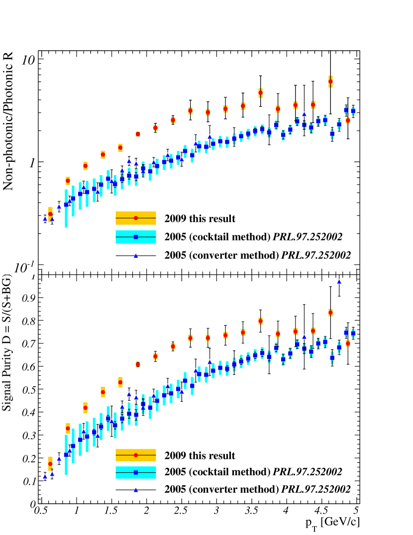
Figure 10: (color online). (top) Ratio between the yields of the nonphotonic electrons and the photonic electrons in the reconstructed tracks. The red circles and the blue squares and triangles represent this analysis result and the previous result Adler et al. (2006b), respectively. The error bars and bands represent the statistic and the systematic uncertainties. (bottom) Signal purity which is a ratio of the yield of the heavy flavor electrons to the total reconstructed electrons.

IV Heavy Flavor Electron Cross Section

Table 2: Relative systematic uncertainties on the cross section due to uncertainties in the total sampled luminosity, trigger efficiencies, and detector acceptance. These systematic uncertainties are globally correlated in all $p_{T}$ regions ($p_{T}>1.25$ GeV/$c$ for the uncertainties on $\epsilon_{{\rm trig}}^{e\rm{|MB}}$).

source	uncertainty
MB trig. cross sect.	$9.6\%$
acceptance $A$	$8\%$
reco. efficiency $\epsilon_{{\rm rec}}$	$6\%$
MB trig. efficiency $\epsilon_{{\rm trig}}^{{\rm MB}}$	$2.5\%$
$e$ trig. efficiency $\epsilon_{{\rm trig}}^{e\rm{|MB}}$	$3.6\%$	in $p_{T}>1.25$ GeV/$c$

The invariant cross section is calculated from

$$E\frac{d^{3}\sigma}{dp^{3}}=\frac{1}{2\pi p_{T}}\frac{1}{L}\frac{1}{A\epsilon_{{\rm rec}}\epsilon_{{\rm trig}}}\frac{N(\Delta p_{T},\Delta y)}{\Delta p_{T}\Delta y},$$ (10)

where $L$ denotes the integrated luminosity, $A$ the acceptance, $\epsilon_{{\rm rec}}$ the reconstruction efficiency, $\epsilon_{{\rm trig}}$ the trigger efficiency, and $N$ the estimated number of heavy flavor electrons.

The luminosity, $L$, was calculated from the number of MB events divided by the cross section for the MB trigger. For the latter, a value of $23.0$ mb with a systematic uncertainty of $9.6$% was estimated from van-der-Merr scan results Adler et al. (2003) corrected for the relative changes in the BBC performance. The combination of the acceptance and the reconstruction efficiency, $A\epsilon_{{\rm rec}}(p_{T})$, was estimated by a geant3 simulation. We found that $A\epsilon_{{\rm rec}}(p_{T})$ has a value of $4.7\%\times(1\pm 8\times 10^{-2}(\rm{acc.})\pm 6\times 10^{-2}(\rm{reco.}))$, with a slight $p_{T}$ dependence.

The efficiency of the MB trigger for the hard scattering processes, including heavy flavor electron production, is $\epsilon_{{\rm trig}}^{{\rm MB}}=79.5\%\times(1\pm 2.5\times 10^{-2})$. The efficiency of the electron trigger for the electrons under the condition of the MB trigger firing, $\epsilon_{{\rm trig}}^{e\rm{|MB}}(p_{T})\equiv\epsilon_{{\rm trig}}(p_{T})/\epsilon_{{\rm trig}}^{{\rm MB}}$, can be calculated by the ratio of the number of the reconstructed electrons in the MB triggered sample in coincidence with the electron trigger to the number of the reconstructed electrons without the coincidence. The efficiency $\epsilon_{{\rm trig}}^{e\rm{|MB}}$ is shown in Fig. 11 as a function of $p_{T}$. Whereas we used the calculated efficiency values for the momentum region of $p_{T}<1.25$ GeV/$c$, we assumed a saturated efficiency for $p_{T}>1.25$ GeV/$c$ and estimated the value with a fitting as shown in Fig. 11. The fitting result is $\epsilon_{\rm{plateau}}=56.5\%\times(1\pm 3.6\times 10^{-2})$. The total trigger efficiency $\epsilon_{{\rm trig}}(p_{T})$ can be calculated with the above two efficiencies as $\epsilon_{{\rm trig}}(p_{T})=\epsilon_{{\rm trig}}^{{\rm MB}}\times\epsilon_{{\rm trig}}^{e\rm{|MB}}(p_{T})$. Table 2 summarizes the systematic uncertainties on the cross section due to uncertainties in the total sampled luminosity, trigger efficiencies, and detector acceptance. All systematic uncertainties listed in Table 2 are globally correlated over whole $p_{T}$ region ($p_{T}>1.25$ GeV/$c$ for the uncertainties on $\epsilon_{{\rm trig}}^{e\rm{|MB}}$).

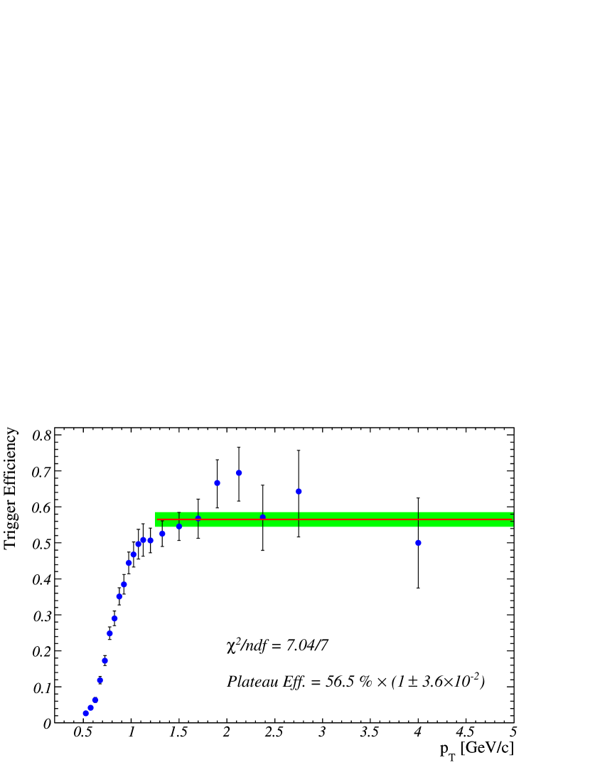
Figure 11: (color online). Efficiency of the electron trigger for reconstructed electrons under the condition that the MB trigger was issued. The red line represents the fitting result with the constant function and the green band represents the fitting uncertainty.

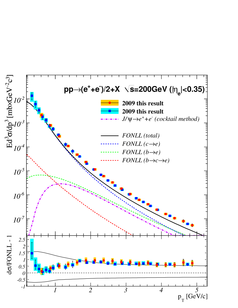
Figure 12: (color online). (top) Invariant differential cross sections of electrons from heavy-flavor decays. The red circles are this analysis of 2009 data and the blue squares are the previous 2005 data Adler et al. (2006b) for the nonphotonic electron cross sections. The error bars and bands represent the statistical and systematic uncertainties. The scaling uncertainty from the Vernier scan is not included in the error bands because the same uncertainty must be considered for both the results of 2009 and 2005. The purple dashed dotted line is electron cross section from $J/\psi\rightarrow e^{+}+e^{-}$ decays estimated from the cocktail method Adare et al. (2011c). The solid and dashed curves are the FONLL calculations. (bottom) Difference of the ratio of the data and the FONLL calculation from 1. The upper and lower curve shows the theoretical upper and lower limit of the FONLL calculation.

The measured cross section of heavy flavor electrons is shown in Fig. 12 and tabulated in Table 3. A correction for bin width Lafferty and Wyatt (1995) is applied to the $p_{T}$ value of each point. The figure also shows the previously published result Adler et al. (2006b). The new result agrees well with the previous result within the uncertainties. Note that in this paper we employed a new analysis method with the HBD whereas the previous measurement employed different methods, the cocktail method and the converter method. The consistency between these measurements proves that additional photonic backgrounds generated in the HBD material are removed, and that this new analysis method with the HBD is robust.

The electron cross section from $J/\psi\rightarrow e^{+}+e^{-}$ decays estimated by the cocktail method Adare et al. (2011c) and a fixed order next-to-leading log (FONLL) pQCD calculation of the heavy flavor contributions to the electron spectrum Cacciari et al. (2005) are also shown in Fig. 12. The $J/\psi$ contribution to the heavy flavor electrons are less than 2% in $p_{T}<1.25$ GeV/$c$ and increase to $\sim$20% until $p_{T}=5.0$ GeV/$c$. The FONLL pQCD calculation shows that the heavy flavor electrons in the low momentum region are dominated by charm quark decays, and the contribution from bottom quarks in $p_{T}<1.25$ GeV/$c$ is less than 5%.

Table 3: Data table for the cross section result corresponding to Fig. 12.

$p_{T}$	$E\frac{d^{3}\sigma}{dp^{3}}$	stat. error	syst. error
[GeV/$c$]	[mb$\times$GeV-2c3]
0.612	2.12$\times 10^{-3}$	0.04$\times 10^{-3}$	0.47$\times 10^{-3}$
0.864	7.93$\times 10^{-4}$	0.09$\times 10^{-4}$	1.11$\times 10^{-4}$
1.115	2.78$\times 10^{-4}$	0.03$\times 10^{-4}$	0.37$\times 10^{-4}$
1.366	1.09$\times 10^{-4}$	0.02$\times 10^{-4}$	0.13$\times 10^{-4}$
1.617	4.77$\times 10^{-5}$	0.08$\times 10^{-5}$	0.58$\times 10^{-5}$
1.867	2.34$\times 10^{-5}$	0.05$\times 10^{-5}$	0.27$\times 10^{-5}$
2.118	1.15$\times 10^{-5}$	0.04$\times 10^{-5}$	0.13$\times 10^{-5}$
2.369	6.05$\times 10^{-6}$	0.20$\times 10^{-6}$	0.68$\times 10^{-6}$
2.619	3.28$\times 10^{-6}$	0.19$\times 10^{-6}$	0.37$\times 10^{-6}$
2.869	1.82$\times 10^{-6}$	0.11$\times 10^{-6}$	0.20$\times 10^{-6}$
3.120	1.08$\times 10^{-6}$	0.07$\times 10^{-6}$	0.12$\times 10^{-6}$
3.370	6.20$\times 10^{-7}$	0.41$\times 10^{-7}$	0.69$\times 10^{-7}$
3.620	4.07$\times 10^{-7}$	0.26$\times 10^{-7}$	0.45$\times 10^{-7}$
3.870	2.42$\times 10^{-7}$	0.19$\times 10^{-7}$	0.27$\times 10^{-7}$
4.121	1.59$\times 10^{-7}$	0.15$\times 10^{-7}$	0.18$\times 10^{-7}$
4.371	1.07$\times 10^{-7}$	0.11$\times 10^{-7}$	0.12$\times 10^{-7}$
4.621	8.02$\times 10^{-8}$	1.11$\times 10^{-8}$	0.89$\times 10^{-8}$
4.871	5.38$\times 10^{-8}$	0.71$\times 10^{-8}$	0.60$\times 10^{-8}$

V Heavy Flavor Electron Spin Asymmetry

Table 4: Systematic uncertainties by type. The scaling uncertainty denotes an uncertainty on scaling of the raw asymmetry $A_{LL}^{\rm{S+BG}}$ and the offset uncertainty denotes an uncertainty on the absolute value of the asymmetry. The “global” in this table means the uncertainties are globally correlated in all $p_{T}$ regions. The scaling uncertainty is represented as the ratio of the uncertainty to the signal ($\Delta S/S$) given in percent and the offset uncertainty is represented as the absolute value of the uncertainty.

source	uncertainty	type
signal purity $D$	$\sim 6\%$	scaling
polarization ( $\frac{\Delta(P_{B}P_{Y})}{P_{B}P_{Y}}$ )	$8.8\%$	global scaling
relative luminosity $r$	$0.14\times 10^{-2}$	global offset
background asymmetry $A_{LL}^{BG}$	$0.2\times 10^{-2}\times\frac{1-D}{D}$	offset

Since parity is conserved in QCD processes, thereby disallowing finite single spin asymmetries, using Eq. 3 we express the expected electron yields for each beam-helicity combination as

$$\begin{array}[]{l}N_{++}^{\rm{exp}}(N_{0},A_{LL})=N_{0}(1+|P_{\rm{B}}P_{\rm{Y}}|A_{LL})\\ N_{--}^{\rm{exp}}(N_{0},A_{LL})=N_{0}(1+|P_{\rm{B}}P_{\rm{Y}}|A_{LL})/r_{--}\\ N_{+-}^{\rm{exp}}(N_{0},A_{LL})=N_{0}(1-|P_{\rm{B}}P_{\rm{Y}}|A_{LL})/r_{+-}\\ N_{-+}^{\rm{exp}}(N_{0},A_{LL})=N_{0}(1-|P_{\rm{B}}P_{\rm{Y}}|A_{LL})/r_{-+},\end{array}$$ (11)

where $N_{\pm\pm}^{\rm{exp}}(N_{0},A_{LL})$ denote the expected yields for collisions between the blue beam-helicity ($\pm$) and the yellow beam-helicity ($\pm$) and $N_{0}$ is the expected yield in collisions of unpolarized beams under the same integrated luminosity as the $++$ beam-helicity combination. $N_{\pm\pm}^{\rm{exp}}(N_{0},A_{LL})$ are used for fitting functions to estimate $A_{LL}$ as described below. $P_{\rm{B}}$ and $P_{\rm{Y}}$ represent the polarizations of the beams. The beam polarizations are measured with a carbon target polarimeter Jinnouchi et al. , normalized by the absolute polarization measured with a separate polarized atomic hydrogen jet polarimeter Okada et al. (2006, ) at another collision point in RHIC ring. The measured polarizations are about $P=57\%$ with a relative uncertainty of $\Delta P/P=4.7\times 10^{-2}$ in the measurement. The relative luminosities are defined as the ratio of the luminosities in the beam-helicity combinations,

$$\begin{array}[]{l}r_{--}\equiv\frac{L_{++}}{L_{--}}\\ r_{+-}\equiv\frac{L_{++}}{L_{+-}}\\ r_{-+}\equiv\frac{L_{++}}{L_{-+}},\end{array}$$ (12)

where $L_{\pm\pm}$ represent the integrated luminosities in the beam-helicity combinations shown by the subscript. The relative luminosities are determined by the ratios of MB trigger counts in the four beam-helicity combinations.

The double-spin asymmetry for inclusive electrons after applying eID-Cut and npe-Cut, which include not only the heavy flavor electrons (S) but also the background electrons (BG), is determined by simultaneously fitting the yields of electrons in each of the four beam-helicity combinations with the expected values $N_{\pm\pm}^{\rm{exp}}(N_{0},A_{LL})$ from Eq. 11, where $A_{LL}$ and $N_{0}$ are free parameters. To perform the fit, a log likelihood method assuming Poisson distributions with expected values of $N_{\pm\pm}^{\rm{exp}}(N_{0},A_{LL})$ was employed. The fit was performed for electron yields in each fill to obtain the fill-by-fill double-spin asymmetry. We confirmed that all asymmetries in different fills are consistent with each other within their statistical uncertainties and, therefore, the patterns of the crossing helicities in the fills do not affect the asymmetry measurement. The final double-spin asymmetry for inclusive electrons, $A_{LL}^{\rm{S+BG}}(p_{T})$, was calculated as the weighted mean of the fill-by-fill asymmetries.

The double-spin asymmetry in the heavy flavor electron production, $A_{LL}^{\rm{HFe}}$, was determined from

$$A_{LL}^{\rm{HFe}}(p_{T})=\frac{1}{D(p_{T})}A_{LL}^{\rm{S+BG}}(p_{T})-\frac{1-D(p_{T})}{D(p_{T})}A_{LL}^{\rm{BG}}(p_{T})$$ (13)

where $A_{LL}^{\rm{BG}}$ represents the spin asymmetries for the background electron production, and $D$ represents the signal purity defined in Eq. 9 and shown in Fig. 10. As previously discussed, most of the background electrons come from Dalitz decays of the $\pi^{0}$ and $\eta$, or from conversions of photons from decays of those hadrons. The fractional contribution on the partonic level, and therefore the production mechanism for the $\pi^{0}$ and $\eta$ is expected to be very similar up to $\sim 10$ GeV/$c$ Adare et al. (2007); Adare et al. (2011a). We assume identical spectra for double-spin asymmetries of $\pi^{0}$ production and $\eta$ production, and estimated $A_{LL}^{\rm{BG}}$ from only the $\pi^{0}$ double-spin asymmetry using data from this PHENIX measurement. The resulting $A_{LL}^{\rm{BG}}$ is $-0.1\times 10^{-2}<A_{LL}^{\rm{BG}}<0.1\times 10^{-2}$ in $0.5<p_{T}<2.5$ GeV/$c$ and $0.1\times 10^{-2}<A_{LL}^{\rm{BG}}<0.2\times 10^{-2}$ in $2.5<p_{T}<3.0$ GeV/$c$, with uncertainties less than $0.2\times 10^{-2}$.

Systematic uncertainties on $A_{LL}^{\rm{HFe}}$ are separated into scaling uncertainties and offset uncertainties. The scaling uncertainties come from uncertainty in the beam polarizations, $P_{B}$ and $P_{Y}$, and the signal purity, $D$. The uncertainty from the beam polarization is estimated as $\Delta(P_{B}P_{Y})/P_{B}P_{Y}=8.8$% which is globally correlated over the whole $p_{T}$ range. The offset uncertainties come from uncertainties in the relative luminosity, $r$, and the background asymmetry, $A_{LL}^{\rm{BG}}$. The uncertainty from relative luminosity which is also globally correlated over is determined as $\Delta r=1.4\times 10^{-3}$ from comparison of the measured relative luminosities with the MB trigger and the ZDC trigger. The systematic uncertainties are summarized in Table 4.

A transverse double-spin asymmetry $A_{TT}$, which is defined by the same formula as Eq. 2 for the transverse polarizations, can contribute to $A_{LL}$ through the residual transverse components of the beam polarizations. The product of the transverse components of the beam polarization is measured to be $\sim 10^{-2}$ in this experiment. For $\pi^{0}$ production, the $A_{TT}$ is expected to be $\sim 10^{-4}$ based on an NLO QCD calculation Mukherjee et al. (2005). If we assume the transverse asymmetries of $\pi^{0}$ and heavy flavor electrons are comparable, we arrive at the value of $A_{LL}\sim 10^{-6}$. This value is negligible compared with the precision of the $A_{LL}^{S+BG}$ measurement of $\sim 10^{-3}$.

The result of the double-spin asymmetry of heavy flavor electrons is shown in Fig. 13 and tabulated in Table 5. We show systematic uncertainties for scaling and offset separately in the figure. The measured asymmetry is consistent with zero.

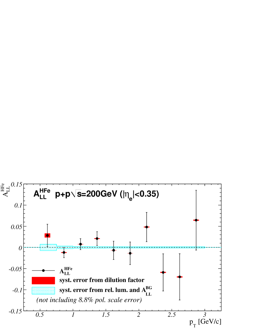
Figure 13: (color online). Double-spin asymmetry of the heavy flavor electron production. The red error bands represent scaling systematic uncertainties from the dilution factor and the blue error bands represents offset systematic uncertainties from relative luminosity and the background spin asymmetry.

Table 5: Data table for the $A_{LL}^{\rm{HFe}}$ result corresponding to Fig. 13.

$p_{T}$[GeV/$c$]	$A_{LL}^{\rm{HFe}}$		stat. uncertainty	syst. uncertainty (offset)	syst. uncertainty (scale)
0.612	2.83$\times 10^{-2}$		2.66$\times 10^{-2}$	0.75$\times 10^{-2}$	0.50$\times 10^{-2}$
0.864	-1.20$\times 10^{-2}$		1.21$\times 10^{-2}$	0.30$\times 10^{-2}$	0.08$\times 10^{-2}$
1.115	0.76$\times 10^{-2}$		1.30$\times 10^{-2}$	0.21$\times 10^{-2}$	0.04$\times 10^{-2}$
1.366	2.08$\times 10^{-2}$		1.63$\times 10^{-2}$	0.18$\times 10^{-2}$	0.10$\times 10^{-2}$
1.617	-0.69$\times 10^{-2}$		2.18$\times 10^{-2}$	0.17$\times 10^{-2}$	0.03$\times 10^{-2}$
1.867	-1.39$\times 10^{-2}$		2.68$\times 10^{-2}$	0.16$\times 10^{-2}$	0.03$\times 10^{-2}$
2.118	4.82$\times 10^{-2}$		3.46$\times 10^{-2}$	0.16$\times 10^{-2}$	0.09$\times 10^{-2}$
2.369	-5.91$\times 10^{-2}$		4.40$\times 10^{-2}$	0.16$\times 10^{-2}$	0.11$\times 10^{-2}$
2.619	-6.97$\times 10^{-2}$		5.47$\times 10^{-2}$	0.16$\times 10^{-2}$	0.13$\times 10^{-2}$
2.869	6.43$\times 10^{-2}$		7.07$\times 10^{-2}$	0.16$\times 10^{-2}$	0.12$\times 10^{-2}$

VI Discussion

In this section, we discuss constraint of $\Delta g$ from the measured double-spin asymmetry with an LO pQCD calculation. In $p$$+$$p$ collisions at $\sqrt{s}=200$ GeV, heavy flavor electrons with momentum ranging $0.50<p_{T}<1.25$ GeV/$c$ are mainly produced by open charm events as described in Sec. IV. Whereas the precise mechanism for $J/\psi$ production is unknown, unpolarized and polarized cross section of the open charm production can be estimated with pQCD calculations. In LO pQCD calculations, only $gg\rightarrow c\bar{c}$ and $q\bar{q}\rightarrow c\bar{c}$ are allowed for the open charm production. The charm quarks are primarily created by the $gg$ interaction in the unpolarized hard scattering. In addition, the anti-quark polarizations are known to be small from semi-inclusive DIS measurements precisely enough that both DSSV de Florian et al. (2009) and GRSV Gl$\ddot{\rm{u}}$ck et al. (2001) expect contribution of polarized $q\bar{q}$ cross section to the double-spin asymmetry of the heavy flavor electrons in $|\eta|<0.35$ and $p_{T}<3.0$ GeV/$c$ to be $\sim 10^{-4}$ Riedl et al. , which is much smaller than the accuracy of this measurement. Therefore, in this analysis of $\Delta g$, we ignore the $q\bar{q}$ interaction and assume the asymmetries are due only to the $gg$ interaction. Under the assumption, the spin asymmetry of the heavy flavor electrons is expected to be approximately proportional to the square of polarized gluon distribution normalized by unpolarized distribution, $|\Delta g/g(x,\mu)|^{2}$.

We estimated the unpolarized and the polarized cross section of charm production in $p$$+$$p$ collisions with a LO pQCD calculation of $gg\rightarrow c\bar{c}$ Karliner and Robinett (1994). For this calculation, CTEQ6M Pumplin et al. (2002) was employed for the unpolarized parton distribution functions (PDF). For the polarized PDF, we assumed $|\Delta g(x,\mu)|=Cg(x,\mu)$ where $C$ is a constant. The charm quark mass was assumed as $m_{c}=$ 1.4 GeV/$c^{2}$ and the factorization scale in CTEQ6 and the renormalization scale were assumed to be identical to $\mu=m_{T}^{c}\equiv\sqrt{{p_{T}^{c}}^{2}+{m_{c}}^{2}}$.

The fragmentation and decay processes were simulated with pythia8 Sjostrand et al. ; Sjostrand et al. (2006). We generated $pp\rightarrow c\bar{c}+X$ events and selected electrons from the charmed hadrons, $D^{+}$, $D^{0}$, $D_{s}$, $\Lambda_{c}$ and their antiparticles. We scaled the charm quark yield in pythia with respect to the pQCD calculated unpolarized and polarized cross sections to obtain unpolarized and polarized electron yields from charmed hadron decays under these cross sections. We also applied a pseudorapidity cut of $|\eta|<0.35$ for the electrons to match the acceptance of the PHENIX central arms. The shape of the expected spin asymmetry $A_{LL}^{\rm{HFe}}(p_{T})$ is then determined from the simulated electron yields.

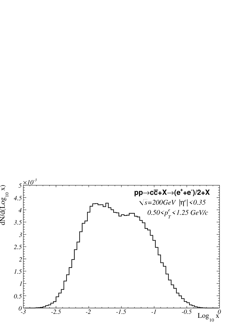
Figure 14: (color online). Bjorken $x$ distributions of gluons contributing the heavy flavor electron production with momentum ranging $0.50<p_{T}<1.25$ GeV/$c$ obtained from pythia simulation. The distribution is normalized with respect to the number of total generated charmed hadrons.

Figure 14 shows the distributions of the gluon Bjorken $x$ contributing to heavy flavor electron production in the momentum range $0.50<p_{T}<1.25$ GeV/$c$, from pythia. Using the mean and the RMS of the distribution for $0.50<p_{T}<1.25$ GeV/$c$, we determine the mean $x$ for heavy flavor electron production to be $\left\langle\log_{10}x\right\rangle=-1.6^{+0.5}_{-0.4}$.

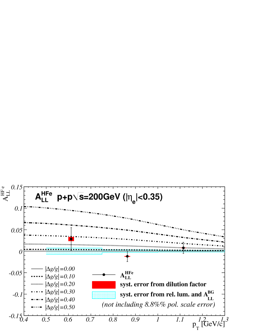
(a) Expected $A_{LL}^{\rm{HFe}}$ for several $|\Delta g/g|$.

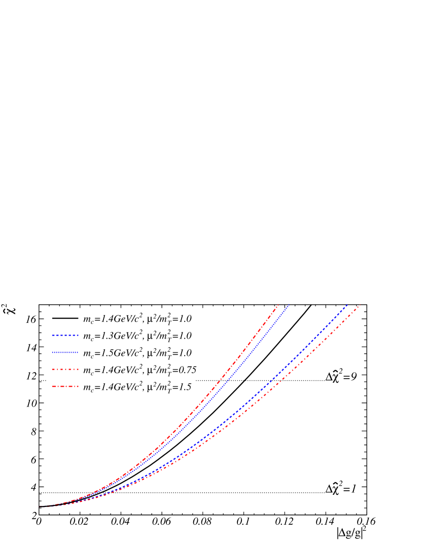
(b) $\hat{\chi}^{2}$ curves.

Figure 15: (color online). (a) $A_{LL}^{\rm{HFe}}$ for $|\Delta g/g|=0.00$, $0.10$, $0.20$, $0.30$, $0.40$, $0.50$ are shown as the solid line, the dashed line, the dotted line, the dashed dotted line, the long-dashed dotted line, the dashed triplicate-dotted line respectively. They are plotted with the measured data points and the notation for the error bars are same as Fig. 13. (b) $\hat{\chi}^{2}$ curves calculated from (a) as a function of $|\Delta g/g|^{2}$. The black solid line is the default configuration. The blue curves are after changing the charm mass to 1.3 GeV/$c^{2}$ (dashed line) and to 1.5 GeV/$c^{2}$ (doted line) and the red curves are after changing the scale $\mu^{2}$ to $0.75{m_{T}^{c}}^{2}$ (dashed dotted line) and $1.5{m_{T}^{c}}^{2}$ (long-dashed dotted line).

We calculated expected $A_{LL}^{\rm{HFe}}(p_{T})$ by varying $C=|\Delta g/g|$. Figure 15(a) shows several of these curves, along with the measured points. $\chi^{2}$ values are calculated for each value of $C$, along with related uncertainties. By assuming that the systematic uncertainties on the points are correlated and represent global shifts, we defined the quantity $\hat{\chi^{2}}$ as

$$\begin{array}[]{rl}\hat{\chi}^{2}(C)&\equiv-2\log\left(\left(2\pi\right)^{\frac{n}{2}}\hat{P}(C)\right)\\ \hat{P}(C)&\equiv\int dpdqN(p)N(q)\times\\ &\prod_{i=1}^{n}N\left(\frac{\left(y_{i}+p\epsilon_{\rm{syst}}^{i\ \rm{offset}}-\left(1+q\gamma_{\rm{syst}}^{i\ \rm{scale}}\right)f(x_{i};C)\right)}{\epsilon_{\rm{stat}}^{i}}\right)\\ &\gamma_{\rm{syst}}^{i\ \rm{scale}}=\sqrt{\left(\frac{\epsilon_{\rm{syst}}^{i\ \rm{scale}}}{y_{i}}\right)^{2}+\left(\frac{\Delta(P_{B}P_{Y})}{P_{B}P_{Y}}\right)^{2}},\\ \end{array}$$

where $N(X)$ denotes normal probability distribution, i.e. $N(X)=1/\sqrt{2\pi}\exp(-X^{2}/2)$, $n$ is the number of the data points and equal to three, and for the $i$-th data point, $x_{i}$ is the $p_{T}$ value, $y_{i}$ is the $A_{LL}$ value, and $\epsilon_{\rm{stat}}^{i}$, $\epsilon_{\rm{syst}}^{i\ \rm{offset}}$ and $\epsilon_{\rm{syst}}^{i\ \rm{scale}}$ represent the statistical, offset systematic and scaling systematic uncertainties, respectively. $f(p_{T};C)$ denotes the expected $A_{LL}(p_{T})$ for the parameter of $C=|\Delta g/g|$. $\Delta(P_{B}P_{Y})$ is an uncertainty for polarization mentioned in Sec. V. If we set the systematic uncertainties, $\epsilon_{\rm{syst}}^{\rm{offset}}$ and $\gamma_{\rm{syst}}^{i\ \rm{scale}}$, to zero, the newly defined $\hat{\chi^{2}}$ is consistent with the conventional $\chi^{2}$.

The resulting $\hat{\chi}^{2}$ curve is shown in Fig. 15(b), plotted as a function of $C^{2}=|\Delta g/g|^{2}$ because the curvature becomes almost parabolic. The minimum of $\hat{\chi}^{2}$, $\hat{\chi}^{2}_{{\rm min}}$, is located at $|\Delta g/g|^{2}=0.0$ which is the boundary of $|\Delta g/g|^{2}$. $\Delta\hat{\chi}^{2}\equiv\hat{\chi}^{2}-\hat{\chi}^{2}_{{\rm min}}=1$ and $9$ were utilized to determine $1\sigma$ and $3\sigma$ uncertainties. With these criteria, we found the constraints on the gluon polarization are $|\Delta g/g(\left\langle\log_{10}x\right\rangle,\mu)|^{2}<3.3\times 10^{-2}$($1\sigma$) and $10.9\times 10^{-2}$($3\sigma$). The constraints are consistent with theoretical expectations for $\Delta g/g(x,\mu)$ at $\left\langle\log_{10}x\right\rangle=-1.6^{+0.5}_{-0.4}$ and $\mu=1.4$ GeV which are $\sim-0.006$ from DSSV, $\sim 0.016$ from GRSV(std) and $\sim 0.019$ from GRSV(val) using CTEQ6 for the unpolarized PDF.

The effects of the charm quark mass and scale factor in the cross section calculation were also checked by varying the charm mass from $m_{c}=1.3$ GeV/$c^{2}$ to 1.5 GeV/$c^{2}$ and the scale to $\mu^{2}=0.75{m_{T}^{c}}^{2}$ and $1.5{m_{T}^{c}}^{2}$. Figure 15(b) also shows the resulting $\hat{\chi}^{2}$ curves. Considering the variation of the crossing position at $\Delta\hat{\chi}^{2}=1$, the constraint including the uncertainties from the charm mass and the scale can be represented as $|\Delta g/g|^{2}<(3.3_{-0.3}^{+0.4}{\rm{(mass)}}_{-0.4}^{+0.7}{\rm{(scale)}})\times 10^{-2}$($1\sigma$).

The integral of the CTEQ6 unpolarized PDF in the sensitive $x$ region of $\left\langle\log_{10}x\right\rangle=-1.6^{+0.5}_{-0.4}$ and $\mu=1.4$ GeV is $\int_{0.01}^{0.08}dxg(x,\mu)=4.9$. Hence the constraint on the integral of the polarized PDF at $1\sigma$ corresponds to $|\int_{0.01}^{0.08}dx\Delta g(x,\mu)|<0.85$. This study also highlights the possibility for constraining $\Delta g$ in this Bjorken $x$ region more precisely in the future with higher statistics and higher beam polarizations.

VII Summary

We have presented a new analysis method for identifying heavy flavor electrons at PHENIX. With this new method, the signal purity is improved by a factor of about 1.5 around $0.75\lower 2.15277pt\hbox{$\;\buildrel<\over{\sim}\;$}p_{T}\lower 2.15277pt\hbox{$\;\buildrel<\over{\sim}\;$}2.00$ GeV/$c$ due to the rejection of photonic electrons by the HBD. We have reported on the first measurement of the longitudinal double-spin asymmetry of heavy flavor electrons, which are consistent with zero. Using this result, we estimate a constraint of $|\Delta g/g(\log_{10}x=-1.6^{+0.5}_{-0.4},\mu=m_{T}^{c})|^{2}<3.3\times 10^{-2}$($1\sigma$). This value is consistent with the existing theoretical expectations with GRSV and DSSV. With improved statistics and polarization, the helicity asymmetry of heavy flavor electron production can provide more significant constraints on the gluon polarization, and complement other measurements of $\Delta G$.

References

- Ashman et al. (1988) J. Ashman et al. (European Muon Collaboration), Phys. Lett. B 206, 364 (1988).
- Ashman et al. (1989) J. Ashman et al. (European Muon Collaboration), Nucl. Phys. B 328, 1 (1989).
- Ellis and Jaffe (1974) J. Ellis and R. L. Jaffe, Phys. Rev. D 9, 1444 (1974).
- Kodaira (1980) J. Kodaira, Nucl. Phys. B 165, 129 (1980).
- D. Bass (1989) S. D. Bass, The Spin Structure of the Proton (World Scientific, 1989).
- Airapetian et al. (2007) A. Airapetian et al. (HERMES Collaboration), Phys. Rev. D 75, 012007 (2007).
- Alexakhin et al. (2007a) V. Y. Alexakhin et al. (COMPASS Collaboration), Phys. Lett. B 647, 330 (2007a).
- Alexakhin et al. (2007b) V. Y. Alexakhin et al. (COMPASS Collaboration), Phys. Lett. B 647, 8 (2007b).
- Adare et al. (2009a) A. Adare et al. (PHENIX Collaboration), Phys. Rev. Lett. 103, 012003 (2009a).
- Adare et al. (2007) A. Adare et al. (PHENIX Collaboration), Phys. Rev. D 76, 051106 (2007).
- Adler et al. (2006a) S. S. Adler et al. (PHENIX Collaboration), Phys. Rev. D 73, 091102 (2006a).
- Adare et al. (2009b) A. Adare et al. (PHENIX Collaboration), Phys. Rev. D 79, 012003 (2009b).
- Adare et al. (2011a) A. Adare et al. (PHENIX Collaboration), Phys. Rev. D 83, 032001 (2011a).
- (14) P. Djawotho et al. (STAR Collaboration), arXiv:1106.5769 (2011).
- Abelev et al. (2008) B. I. Abelev et al. (STAR Collaboration), Phys. Rev. Lett. 100, 232003 (2008).
- Adare et al. (2011b) A. Adare et al. (PHENIX Collaboration), Phys. Rev. D 84, 012006 (2011b).
- Airapetian et al. (2005) A. Airapetian et al. (HERMES Collaboration), Phys. Rev. D 71, 012003 (2005).
- Alekseev et al. (2008) M. Alekseev et al. (COMPASS Collaboration), Phys. Lett. B 660, 458 (2008).
- de Florian et al. (2009) D. de Florian, R. Sassot, M. Stratmann, and W. Vogelsang, Phys. Rev. D 80, 034030 (2009).
- Karliner and Robinett (1994) M. Karliner and R. W. Robinett, Phys. Lett. B 324, 209 (1994).
- Bojak and Stratmann (2003) I. Bojak and M. Stratmann, Phys. Rev. D 67, 034010 (2003).
- (22) I. Bojak, hep-ph/0005120 (2000).
- (23) J. Riedl, A. Schafer, and M. Stratmann, arXiv:0911.2146 (2009).
- Adler et al. (2006b) S. S. Adler et al. (PHENIX Collaboration), Phys. Rev. Lett. 96, 032001 (2006b).
- Adare et al. (2011c) A. Adare et al. (PHENIX Collaboration), Phys. Rev. C 84, 044905 (2011c).
- Adcox et al. (2003a) K. Adcox et al., Nucl. Instrum. Methods Phys. Res. , Sect. A 499, 469 (2003a).
- Adcox et al. (2003b) K. Adcox et al., Nucl. Instrum. Methods Phys. Res. , Sect. A 499, 480 (2003b).
- Adcox et al. (2003c) K. Adcox et al., Nucl. Instrum. Methods Phys. Res. , Sect. A 499, 489 (2003c).
- Aizawa et al. (2003) M. Aizawa et al., Nucl. Instrum. Methods Phys. Res. , Sect. A 499, 508 (2003).
- Aphecetche et al. (2003) L. Aphecetche et al., Nucl. Instrum. Methods Phys. Res. , Sect. A 499, 521 (2003).
- Akikawa et al. (2003) H. Akikawa et al., Nucl. Instrum. Methods Phys. Res. , Sect. A 499, 537 (2003).
- Allen et al. (2003) M. Allen et al., Nucl. Instrum. Methods Phys. Res. , Sect. A 499, 549 (2003).
- Kazlov et al. (2004) A. Kazlov et al., Nucl. Instrum. Methods Phys. Res. , Sect. A 523, 345 (2004).
- Anderson et al. (2011) W. Anderson et al., Nucl. Instrum. Methods Phys. Res. , Sect. A 646, 35 (2011).
- GEA (1994) GEANT 3. 2. 1 Manual, http://wwwasdoc.web.cern.ch/wwwasdoc/pdfdir/geant.pdf (1994).
- Adare et al. (2011d) A. Adare et al. (PHENIX Collaboration), Phys. Rev. D 83, 052004 (2011d).
- Adler et al. (2003) S. S. Adler et al. (PHENIX Collaboration), Phys. Rev. Lett. 91, 241803 (2003).
- Lafferty and Wyatt (1995) G. D. Lafferty and T. R. Wyatt, Nucl. Instrum. Methods Phys. Res. , Sect. A 355, 541 (1995).
- Cacciari et al. (2005) M. Cacciari, P. Nason, and R. Vogt, Phys. Rev. Lett. 95, 122001 (2005).
- (40) O. Jinnouchi et al., nucl-ex/0412053 (2004).
- Okada et al. (2006) H. Okada et al., Phys. Lett. B 638, 450 (2006).
- (42) H. Okada et al., arXiv:0712.1389 (2007).
- Mukherjee et al. (2005) A. Mukherjee, M. Stratmann, and W. Vogelsang, Phys. Rev. D 72, 034011 (2005).
- Glck et al. (2001) M. Glck, E. Reya, M. Stratmann, and W. Vogelsang, Phys. Rev. D 63, 094005 (2001).
- Pumplin et al. (2002) J. Pumplin et al., JHEP 07, 012 (2002).
- (46) T. Sjostrand et al., arXiv:0710.3820 (2007).
- Sjostrand et al. (2006) T. Sjostrand et al., JHEP 0605, 026 (2006).