Stochastic solutions with derivatives and non-polynomial terms: The scrape-off layer equations

Abstract

The construction of stochastic solutions for nonlinear partial differential equations is a powerful method to obtain new exact results and to develop efficient numerical algorithms, in particular when domain decomposition techniques are used.

This paper deals with the problems that arise when the nonlinear terms are nonpolynomial or involve derivatives. A set of equations of relevance for plasma physics is used as a testing ground for these problems.

1 Introduction

A stochastic solution of a linear or nonlinear partial differential equation is a stochastic process which, when started from a particular point in the domain generates after a time $t$ a boundary measure which, integrated over the initial condition at $t=0$, provides the solution at the point $x$ and time $t$. For example for the heat equation

$$\partial_{t}u(t,x)=\frac{1}{2}\frac{\partial^{2}}{\partial x^{2}}u(t,x)\qquad\text{{with}}\qquad u(0,x)=f(x)$$ (1)

the stochastic process is Brownian motion and the solution is

$$u(t,x)=\mathbb{E}_{x}f(X_{t})$$ (2)

$\mathbb{E}_{x}$ meaning the expectation value, starting from $x$, of the process

$$dX_{t}=dB_{t}$$ (3)

The domain here is $\mathbb{R}\times\left[0,t\right)$ and the expectation value in (2) is the inner product $\left\langle\mu_{t},f\right\rangle$ of the initial condition $f$ with the measure $\mu_{t}$ generated by the Brownian motion at the $t-$boundary. An important condition for the stochastic process (Brownian motion in this case) to be considered the solution of the equation is the fact that the same process works for any initial condition. This should be contrasted with stochastic processes constructed from particular solutions.

That the solutions of linear elliptic and parabolic equations, both with Cauchy and Dirichlet boundary conditions, have a probabilistic interpretation is a classical result and a standard tool in potential theory [1] [2] [3]. In contrast with the linear problems, explicit solutions in terms of elementary functions or integrals for nonlinear partial differential equations are only known in very particular cases. Therefore the construction of solutions through stochastic processes, for nonlinear equations, has become an active field in recent years. The first stochastic solution for a nonlinear PDE was constructed by McKean [4] for the KPP equation. Later on, the exit measures provided by diffusion plus branching processes [5] [6] as well as the stochastic representations recently constructed for the Navier-Stokes [7] [8] [9] [10] [11], the Vlasov-Poisson [12] [13] [15], the Euler [14] and a fractional version of the KPP equation [16] define solution-independent processes for which the mean values of some functionals are solutions to these equations. Therefore, they are exact stochastic solutions.

In the stochastic solutions one deals with a process that starts from the point where the solution is to be found, a functional being then computed when the process reaches the boundary. In addition to providing new exact results, the stochastic solutions are also, in some cases, a promising tool for numerical implementation. This is because stochastic simulation only grows with the dimension of the process, whereas a deterministic algorithm grows exponentially with the dimension of the space. In addition, because of the independence of the sample paths of the process, they are a natural choice for parallel and distributed computation.

Stochastic algorithms are also used for domain decomposition purposes [17] [18] [19]. One decomposes the space in subdomains and then uses in each one a deterministic algorithm with Dirichlet boundary conditions, the values on the boundaries being determined by a stochastic algorithm, thus minimizing the time-consuming communication problem between domains.

There are basically two methods to construct stochastic solutions. The first method, which will be called the McKean method, is essentially a probabilistic interpretation of the Picard series. The differential equation is written as an integral equation which is rearranged in a such a way that the coefficients of the successive terms in the Picard iteration obey a normalization condition. The Picard iteration is then interpreted as an evolution and branching process, the stochastic solution being equivalent to importance sampling of the normalized Picard series. The second method constructs the boundary measures of a measure-valued stochastic process (a superprocess) and obtain the solutions of the differential equation by a scaling procedure. For a comparison of the two methods refer to [20].

To extend the construction of stochastic solutions to cases more general than those dealt with in the past, techniques must be developed to handle derivatives and nonpolynomial interactions. Sometimes the direct handling of derivatives may be avoided if the derivative of the propagation kernel is smooth. This is the case in the configuration space Navier-Stokes equation [10], where by an integration by parts the derivative of the heat kernel is controlled by a majorizing kernel and absorbed in the probability measure. However, in general, this is not possible.

In this paper, the construction of stochastic solutions, for differential equations involving derivatives and nonpolynomial interactions, will be carried out for two systems of equations which describe plasma turbulence in the scrape-off layer. In both cases we deal with the Cauchy problem, namely the equations are defined in the full space with initial conditions at $t=0$. This is the most natural setting when the McKean approach is used. Spatial boundary conditions are easier to implement through the superprocess formulation, with or without a scaling limit (see [20]).

2 A system of scrape-off layer equations (SOLEDGE 2D)

The SOLEDGE-2D equations are [21]

$$\partial_{t}N+\frac{1}{q}\partial_{\theta}\Gamma+\frac{\chi}{\eta}N = D\partial_{r}^{2}N$$

$$\partial_{t}\Gamma+\frac{1}{q}\left(1-\chi\right)\partial_{\theta}\left(\frac{\Gamma^{2}}{N}+N\right)+\frac{\chi}{\eta}\left(\Gamma-\Gamma_{0}\right) = \nu\partial_{r}^{2}\Gamma$$ (4)

where $\Gamma$ and $N$ are the dimensionless parallel momentum and density, $\left(r,\theta\right)$ are the radial and poloidal coordinates and the mask function $\chi$ equals one in a region where an obstacle is located and zero elsewhere.

To construct a stochastic representation for the solution one needs to identify a stochastic process associated to the linear component (to the full linear component or part of it) and then, through an integral equation, construct the branching mechanism representing the nonlinear part.

2.1 The linear part, $\chi=0$

The linear part of the system for $\chi=0$ is:

$$\partial_{t}N+\frac{1}{q}\partial_{\theta}\Gamma = D\partial_{r}^{2}N$$

$$\partial_{t}\Gamma+\frac{1}{q}\partial_{\theta}N = \nu\partial_{r}^{2}\Gamma$$ (5)

Given the initial conditions at time zero $\left(\begin{array}[]{l}N\left(0,r,\theta\right)\\ \Gamma\left(0,r,\theta\right)\end{array}\right)$ the solution of this system is

$$\left(\begin{array}[]{l}N\left(t,r,\theta\right)\\ \Gamma\left(t,r,\theta\right)\end{array}\right)=\exp t\left\{-\frac{1}{q}A\partial_{\theta}+B\partial_{r}^{2}\right\}\left(\begin{array}[]{l}N\left(0,r,\theta\right)\\ \Gamma\left(0,r,\theta\right)\end{array}\right)$$ (6)

$A$ and $B$ being the matrices

$$A=\left(\begin{array}[]{ll}0&1\\ 1&0\end{array}\right);\hskip 8.5359ptB=\left(\begin{array}[]{ll}D&0\\ 0&\nu\end{array}\right)$$

With $x\circeq\left(r,\theta\right)$, define a function $F$ such that

$$F\left(x,i\right) = N\left(x\right)\hskip 8.5359pt\text{if}\hskip 8.5359pti=+1$$

$$F\left(x,i\right) = \Gamma\left(x\right)\hskip 8.5359pt\text{if}\hskip 8.5359pti=-1$$ (7)

Associated to the equations (5) there is an operator $\mathcal{O}$

$$\left(\mathcal{O}F\right)\left(x,i\right)=\frac{1}{2}\left\{2D\delta_{i,1}+2\nu\delta_{i,-1}\right\}\partial_{r}^{2}F\left(x,i\right)-\frac{1}{q}\delta_{i,-j}\partial_{\theta}F\left(x,j\right)$$ (8)

which is the generator of the stochastic process associated to the full linear part of the equation.

However, for the construction of a stochastic solution to the nonlinear equation through a probabilistic interpretation of the integral equation, it is convenient to have a stochastic process that operates in a simple way on the arguments of the function. Therefore instead of the process associated to $\mathcal{O}$, only the diffusion associated to the first term in (8) will be used below. It also provides an easier handling of the $\partial_{\theta}$ derivative.

2.2 The $\chi=1$ case

In the $\chi=1$ case the equation (4) is linear

$$\partial_{t}N+\frac{1}{q}\partial_{\theta}\Gamma+\frac{1}{\eta}N = D\partial_{r}^{2}N$$

$$\partial_{t}\Gamma+\frac{1}{\eta}\left(\Gamma-\Gamma_{0}\right) = \nu\partial_{r}^{2}\Gamma$$ (9)

the solution being

$$\left(\begin{array}[]{l}N\left(t\right)\\ \Gamma\left(t\right)\end{array}\right) = e^{t\left(-\frac{1}{q}C\partial_{\theta}+B\partial_{r}^{2}-\frac{1}{\eta}\right)}\left\{\left(\begin{array}[]{l}N\left(0\right)\\ \Gamma\left(0\right)\end{array}\right)\right.$$ (17)

$$+\left.\int_{0}^{t}d\tau e^{-\tau\left(-\frac{1}{q}C\partial_{\theta}+B\partial_{r}^{2}-\frac{1}{\eta}\right)}\left(\begin{array}[]{c}0\\ \frac{\Gamma_{0}}{\eta}\end{array}\right)\right\}$$

with $B$ defined before and $C$ being the matrix

$$C=\left(\begin{array}[]{ll}0&1\\ 0&0\end{array}\right)$$

2.3 The nonlinear equations $\left(\chi=0\right)$: A stochastic solution

For the nonlinear equations one writes

$$N\left(t,r,\theta\right) = e^{tD\partial_{r}^{2}}N\left(0,r,\theta\right)-\frac{1}{q}\int_{0}^{t}d\tau e^{\tau D\partial_{r}^{2}}\partial_{\theta}\Gamma\left(t-\tau,r,\theta\right)$$

$$\Gamma\left(t,r,\theta\right) = e^{t\nu\partial_{r}^{2}}\Gamma\left(0,r,\theta\right)-\frac{1}{q}\int_{0}^{t}d\tau e^{\tau\nu\partial_{r}^{2}}\partial_{\theta}\left\{\frac{\Gamma^{2}}{N}+N\right\}\left(t-\tau,r,\theta\right)$$

Denote by $\xi_{s}^{(N)}$ and $\xi_{s}^{(\Gamma)}$ two Brownian motions in the $r-$coordinate with diffusion coefficients $\sqrt{2D}$ and $\sqrt{2\nu}$. Then the equations (LABEL:2.6) may be reinterpreted as defining a probabilistic processes for which the expectation values are the functions $N\left(t,r,\theta\right)$ and $\Gamma\left(t,r,\theta\right)$, that is

$$N\left(t,r,\theta\right) = \mathbb{E}_{\left(t,r,\theta\right)}\left[p\frac{1}{p}N\left(0,\xi_{t}^{(N)},\theta\right)-\frac{t}{q\left(1-p\right)}\int_{0}^{t}\frac{1-p}{t}d\tau\partial_{\theta}\Gamma\left(t-\tau,\xi_{\tau}^{(N)},\theta\right)\right]$$

$$\Gamma\left(t,r,\theta\right) = \mathbb{E}_{\left(t,r,\theta\right)}\left[p\frac{1}{p}\Gamma\left(0,\xi_{t}^{(\Gamma)},\theta\right)-\frac{2t}{q\left(1-p\right)}\int_{0}^{t}\frac{1-p}{t}d\tau\partial_{\theta}\left\{\frac{1}{2}\frac{\Gamma^{2}}{N}+\frac{1}{2}N\right\}\left(t-\tau,\xi_{\tau}^{(\Gamma)},\theta\right)\right]$$

$\mathbb{E}_{\left(t,r,\theta\right)}$ denotes the expectation value of a stochastic process started from $\left(t,r,\theta\right)$. The processes that construct the solution at the point $\left(t,r,\theta\right)$ are backwards-in-time processes that start from time $t$ and propagate to time zero. With probability $p$ the processes reach time zero and the contribution to the expectation value is $\frac{1}{p}N\left(0,\xi_{t}^{(N)},\theta\right)$ (or $\frac{1}{p}\Gamma\left(0,\xi_{t}^{(\Gamma)},\theta\right)$). With probability $\left(1-p\right)$ the process is interrupted at a time $\tau$ chosen with uniform probability in the interval $\left(t,0\right)$. For the process associated to $N$, the process changes its nature, becomes a $\Gamma$ process and picks up a factor $-\frac{t}{q\left(1-p\right)}$. For the case of the process $\Gamma$, with probability $\frac{1}{2}$, this process either changes to a $N$ process or branches into a $N$ and a $\Gamma$ process. In both cases it picks up a factor $-\frac{2t}{q\left(1-p\right)}$.

Notice that the propagation process acts only on the $r-$coordinate. Therefore the derivative $\partial_{\theta}$, the square in $\Gamma^{2}$ and the quotient in $\frac{\Gamma^{2}}{N}$ may all be treated as operators which are kept as labels at each branching point. When all the lines of the process reach time zero, the initial condition is sampled at the arrival $r_{0}-$coordinate. This initial condition is not simply a value but a function of $\theta$ ($\Gamma\left(0,r_{0},\theta\right)$ or $N\left(0,r_{0},\theta\right)$). It implies that both the initial condition and all its derivatives at the argument $\theta$ must be provided. This initial functions are then backtracked throughout the sample lines, the multiplicative factors are picked up at each $\tau$ interrupt and the operators applied whenever a labelled branching point is reached. This provides the contribution of each sample path to the expectation value. Figure 1 displays an example of a sample path, where the operators picked up along the way are denoted by flags.

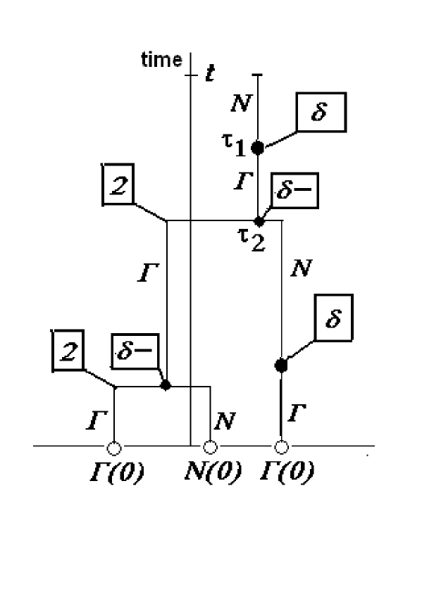
Figure 1: A sample path of the $N-\Gamma$ stochastic process

Notice the order of the operators at each branching point. For example, at the leftmost $\delta-$ labelled point the operation is

$$\partial_{\theta}\left\{\frac{\Gamma^{2}\left(0,r_{0}^{(1)},\theta\right)}{N\left(0,r_{0}^{(2)},\theta\right)}\right\}$$

and the whole contribution of this sample path to the $N-$expectation value is

$$\partial_{\theta}^{2}\left\{\left(\partial_{\theta}\left\{\frac{\Gamma^{2}\left(0,r_{0}^{(1)},\theta\right)}{N\left(0,r_{0}^{(2)},\theta\right)}\right\}\right)^{2}\left\{\partial_{\theta}\Gamma\left(0,r_{0}^{(3)},\theta\right)\right\}^{-1}\right\}$$

times the factor $\left(\frac{1}{p}\right)^{3}\frac{4t\tau_{1}\tau_{2}^{2}}{q^{4}\left(1-p\right)^{4}}$.

If the initial conditions $\left|\frac{\Gamma^{2}}{N},N,\Gamma\right|$ and all its derivatives are bound by a constant $M$, a worst case analysis implies that almost sure convergence of the expectation value is guaranteed for

$$\frac{t}{q}M<1$$

However, in practice, this condition is too severe.

3 A two-dimensional fluid model for the scrape-off layer (TOKAM 2D)

Here both the configuration and the Fourier space equations will be analyzed.

3.1 The configuration space equations

A two-dimensional fluid model for the scrape-off layer based on the interchange instability (TOKAM 2D [22]) is

$$\begin{array}[]{lll}\frac{\partial}{\partial t}n&=&S-\{\phi,n\}-\sigma ne^{\Lambda-\phi}+D\Delta_{\bot}n\\ \frac{\partial}{\partial t}\Delta_{\bot}\phi&=&\sigma\left(1-e^{\Lambda-\phi}\right)+\nu\Delta_{\bot}^{2}\phi-\{\phi,\Delta_{\bot}\phi\}-\frac{1}{n}g\partial_{x_{2}}n\end{array}$$ (20)

where $n=\frac{N}{N_{0}}$ is the normalized density field and $\phi=\frac{eU}{T_{e}}$ the normalized electric potential. The brackets $\left\{\cdots\right\}$ are Poisson brackets, $\left\{f,g\right\}=\partial_{x_{1}}f\partial_{x_{2}}g-\partial_{x_{2}}f\partial_{x_{1}}g$, with $x_{1}=\left(r-a\right)/\rho_{s}$ the minor radius normalized by the Larmor radius $\rho_{s}^{2}=T_{e}/m_{i}$ and $x_{2}=a\theta/\rho_{s}$, $a$ being the plasma radius. $S$ is a source term.

The first equation is rewritten as

$$\begin{array}[]{lll}\frac{\partial}{\partial t}n&=&-\sigma e^{\Lambda}n+D\Delta_{\bot}n+S-\{\phi,n\}-\sigma e^{\Lambda}\sum_{j=1}\frac{\left(-1\right)^{j}}{j!}n\phi^{j}\end{array}$$ (21)

the first two (linear) terms generating the propagating part of the stochastic process and the others the branching.

The second equation involves $\phi\left(x\right),\Delta_{\bot}\phi\left(x\right)$ and $\Delta_{\bot}^{2}\phi\left(x\right)$. Because the time derivative acts on $\Delta_{\bot}\phi\left(x\right)$ it is natural to choose this term as the basic variable. Define

$$\Psi\left(x\right)=\Delta_{\bot}\phi\left(x\right)$$ (22)

Then with

$$K\left(x-y\right)=\frac{1}{2\pi}\log\left|x-y\right|$$ (23)

$$\phi\left(x\right)=\left(K\Psi\right)\left(y\right)=\int d^{2}yK\left(x-y\right)\Psi\left(y\right)$$ (24)

the second equation in (20) becomes

$$\frac{\partial}{\partial t}\Psi = -\sigma e^{\Lambda}\Psi+\nu\Delta_{\bot}\Psi+\sigma\left(1-e^{\Lambda}\right)+\sigma e^{\Lambda}\left(K+\delta\right)\Psi$$ (25)

$$-\sigma e^{\Lambda}\sum_{j=2}\frac{\left(-1\right)^{j}}{j!}\left(K\Psi\right)^{j}-\{\left(K\Psi\right),\Psi\}-g\partial_{x_{2}}\log n$$

where $\delta$ stands for the kernel $\delta\left(x-y\right)$. Notice that from the negative contribution at $x=y$ of the term $\sigma e^{\Lambda}K\Psi$ (in the expansion of $-\sigma e^{-\phi}$), a negative part is extracted which becomes a local dissipative term.

The integral version of the equations (21) and (25) is

$$n\left(x,t\right) = e^{-t\sigma e^{\Lambda}}e^{tD\Delta_{\bot}}n\left(x,0\right)$$

$$+\int_{0}^{t}dse^{-s\sigma e^{\Lambda}}e^{sD\Delta_{\bot}}\left\{S-\{K\Psi,n\}-\sigma e^{\Lambda}\sum_{j=1}\frac{\left(-1\right)^{j}}{j!}n\left(K\Psi\right)^{j}\right\}\left(x,t-s\right)$$

$$\Psi\left(x,t\right) = e^{-t\sigma e^{\Lambda}}e^{t\nu\Delta_{\bot}}\Psi\left(x,0\right)+\int_{0}^{t}e^{-s\sigma e^{\Lambda}}e^{s\nu\Delta_{\bot}}\left\{\sigma\left(1-e^{\Lambda}\right)+\sigma e^{\Lambda}\left(K+\delta\right)\Psi\right.$$ (27)

$$\left.-\sigma e^{\Lambda}\sum_{j=2}\frac{\left(-1\right)^{j}}{j!}\left(K\Psi\right)^{j}-\{\left(K\Psi\right),\Psi\}-g\partial_{x_{2}}\log n\right\}\left(x,t-s\right)$$

The integral equations will now be given a probabilistic interpretation. In addition to the usual propagation and branching mechanisms, the kernel integrations $\left(K\Psi\right)\left(x\right)=\int d^{2}yK\left(x-y\right)\Psi\left(y\right)$ and $\left(\partial_{x_{i}}K\Psi\right)\left(x\right)$ must also be given a probabilistic interpretation. For this purpose two questions have to be dealt with. First, the kernel integrals $\int d^{2}yK\left(x-y\right)$ and $\int d^{2}y\partial_{x_{i}}K\left(x-y\right)$ are not finite, second $K\left(x-y\right)$ and $\partial_{x_{i}}K\left(x-y\right)$ are not positive definite. A positive function $h\left(y\right)$ is chosen in such a way that

$$N\left(x\right)=\int d^{2}y\left|K\left(x-y\right)\right|h\left(y\right);N_{\delta}\left(x\right)=\int d^{2}y\left|K+\delta\right|h\left(y\right);N_{i}\left(x\right)=\int d^{2}y\left|\partial_{x_{i}}K\right|h\left(y\right)$$

are finite. Then

$$\rho\left(x,y\right) = \frac{\left|K\left(x-y\right)\right|h\left(y\right)}{N\left(x\right)};\rho_{\delta}\left(x,y\right)=\frac{\left|K\left(x-y\right)+\delta\left(x-y\right)\right|h\left(y\right)}{N_{\delta}\left(x\right)};$$

$$\rho_{i}\left(x,y\right) = \frac{\left|\partial_{i}K\left(x-y\right)\right|h\left(y\right)}{N_{i}\left(x\right)}$$

may be considered as $x-$dependent probability densities in $y\in\mathbb{R}^{2}$. Define

$$\Omega\left(x,t\right)=\frac{\Psi\left(x,t\right)}{h\left(x\right)}$$

Then, Eqs.(LABEL:3.6) and (27) are rewritten

$$n\left(x,t\right) = e^{-t\sigma e^{\Lambda}}e^{tD\Delta_{\bot}}n\left(x,0\right)+\int_{0}^{t}ds\sigma e^{\Lambda}e^{-s\sigma e^{\Lambda}}e^{sD\Delta_{\bot}}\left\{p_{s,n}M_{s,n}S\left(x\right)\right.$$ (28)

$$\left.+p_{B,n}^{(1)}M_{2,n}\partial_{x_{2}}n\int d^{2}y\rho_{1}\left(x,y\right)\Omega\left(y\right)+p_{B,n}^{(2)}M_{1,n}\partial_{x_{1}}n\int d^{2}y\rho_{2}\left(x,y\right)\Omega\left(y\right)\right.$$

$$\left.+p_{\Sigma,n}\sum_{j=1}p_{j,n}M_{j,n}n\left(x\right)\left(\int d^{2}y\rho\left(x,y\right)\Omega\left(y\right)\right)^{j}\right\}\left(t-s\right)$$

$$\Omega\left(x,t\right) = e^{-t\sigma e^{\Lambda}}e^{t\nu\Delta_{\bot}}\Omega\left(x,0\right)+\int_{0}^{t}ds\sigma e^{\Lambda}e^{-s\sigma e^{\Lambda}}e^{s\nu\Delta_{\bot}}\left\{p_{k}M_{k}+p_{\delta}M_{\delta}\int d^{2}y\rho_{\delta}\left(x,y\right)\Omega\left(y\right)\right.$$

$$\left.+p_{\Sigma,\Omega}\sum_{j=2}p_{j,\Omega}M_{j,\Omega}\left(\int d^{2}y\rho\left(x,y\right)\Omega\left(y\right)\right)^{j}\right.$$

$$\left.+p_{B,\Omega}^{(1)}\left(\frac{1}{2}M_{2,\Omega}^{(a)}\partial_{x_{2}}\Omega+\frac{1}{2}M_{2,\Omega}^{(b)}\Omega\right)\int d^{2}y\rho_{1}\left(x,y\right)\Omega\left(y\right)\right.$$

$$\left.+p_{B,\Omega}^{(2)}\left(\frac{1}{2}M_{1,\Omega}^{(a)}\partial_{x_{1}}\Omega+\frac{1}{2}M_{1,\Omega}^{(b)}\Omega\right)\int d^{2}y\rho_{2}\left(x,y\right)\Omega\left(y\right)+p_{g}M_{g}\partial_{x_{2}}\log n\right\}\left(t-s\right)$$

with probabilities

$$p_{s,n} = \left(3+\sigma e^{\Lambda}\right)^{-1}$$

$$p_{B,n}^{(1)} = p_{B,n}^{(2)}=\left(3+\sigma e^{\Lambda}\right)^{-1}$$

$$p_{\Sigma,n} = \sigma e^{\Lambda}\left(3+\sigma e^{\Lambda}\right)^{-1}$$

$$p_{j,n} = \frac{1}{j!\left(e-1\right)}$$

$$p_{k} = \left(2+\sigma+2\sigma e^{\Lambda}+g\right)^{-1}$$

$$p_{B,\Omega}^{(1)} = p_{B,\Omega}^{(2)}=\left(2+\sigma+2\sigma e^{\Lambda}+g\right)^{-1}$$

$$p_{\delta} = \sigma e^{\Lambda}\left(2+\sigma+2\sigma e^{\Lambda}+g\right)^{-1}$$

$$p_{\Sigma,\Omega} = \sigma e^{\Lambda}\left(2+\sigma+2\sigma e^{\Lambda}+g\right)^{-1}$$

$$p_{g} = g\left(2+\sigma+2\sigma e^{\Lambda}+g\right)^{-1}$$

$$p_{j,\Omega} = \frac{1}{j!\left(e-2\right)}$$ (30)

and multipliers

$$M_{s,n} = 1+3/\left(\sigma e^{\Lambda}\right)$$

$$M_{2,n} = -N_{1}\left(x\right)\left(1+3/\left(\sigma e^{\Lambda}\right)\right)$$

$$M_{1,n} = N_{2}\left(x\right)\left(1+3/\left(\sigma e^{\Lambda}\right)\right)$$

$$M_{j,n} = -\left(-1\right)^{j}\left(e-1\right)\left(1+3/\left(\sigma e^{\Lambda}\right)\right)N\left(x\right)^{j}$$

$$M_{k} = \left(1-e^{\Lambda}\right)\left(2+\sigma+2\sigma e^{\Lambda}+g\right)\left(h\left(x\right)\sigma e^{\Lambda}\right)^{-1}$$

$$M_{2,\Omega}^{(a)} = -2\left(2+\sigma+2\sigma e^{\Lambda}+g\right)N_{1}\left(x\right)\left(\sigma e^{\Lambda}\right)^{-1}$$

$$M_{1,\Omega}^{(a)} = 2\left(2+\sigma+2\sigma e^{\Lambda}+g\right)N_{2}\left(x\right)\left(\sigma e^{\Lambda}\right)^{-1}$$

$$M_{2,\Omega}^{(b)} = -2\left(2+\sigma+2\sigma e^{\Lambda}+g\right)N_{1}\left(x\right)\left(\sigma e^{\Lambda}\right)^{-1}\partial_{x_{2}}\log h\left(x\right)$$

$$M_{1,\Omega}^{(b)} = 2\left(2+\sigma+2\sigma e^{\Lambda}+g\right)N_{2}\left(x\right)\left(\sigma e^{\Lambda}\right)^{-1}\partial_{x_{1}}\log h\left(x\right)$$

$$M_{\delta} = N_{\delta}\left(x\right)\left(2+\sigma+2\sigma e^{\Lambda}+g\right)\left(h\left(x\right)\sigma e^{\Lambda}\right)^{-1}$$

$$M_{g} = -\left(2+\sigma+2\sigma e^{\Lambda}+g\right)\left(h\left(x\right)\sigma e^{\Lambda}\right)^{-1}$$

$$M_{j,\Omega} = -\left(-1\right)^{j}\left(e-2\right)\left(h\left(x\right)\sigma e^{\Lambda}\right)^{-1}\left(2+\sigma+2\sigma e^{\Lambda}+g\right)N\left(x\right)^{j}$$ (31)

In this form the integral equations may be solved by two stochastic process, for $n$ and $\Omega$, which starting from time $t$, propagate backwards-in-time as Brownian motions with diffusion coefficients $D$ and $\nu$, respectively. These processes either reach time zero with probability $e^{-t\sigma e^{\Lambda}}$ or branch at time $t-s$ with probability density $\sigma e^{\Lambda}e^{-s\sigma e^{\Lambda}}$. At each branching point the appropriate branching is chosen according to the probabilities $p_{s,n}$, $p_{B,n}^{(1)}$, $p_{B,n}^{(2)}$, $p_{\Sigma,n}$ for the $n-$process and $p_{k}$, $p_{B,\Omega}^{(1)}$, $p_{B,\Omega}^{(2)}$, $p_{\delta}$, $p_{\Sigma,\Omega}$, $p_{g}$ for the $\Omega-$process. With probability $p_{s,n}$ the $n-$process samples the source $S$ and with probability $p_{k}$ the $\Omega-$process is killed. When it is $\Sigma,n$ or $\Sigma,\Omega$ that is chosen, the branching has $j$ branches according to the probability $p_{j,n}$ or $p_{j,\Omega}$. For the branches of the $n-$type the argument $x$ becomes $x^{\prime}=e^{sD\Delta_{\bot}}x$ or $x^{\prime}=e^{s\nu\Delta_{\bot}}x$, that is, it is propagated by the Brownian motions. For the branches of $\Omega-$type the argument $y$ is chosen with $x-$dependent probability densities $\rho(x,y),\rho_{\delta}\left(x,y\right)$ or $\rho_{i}\left(x,y\right)$. At each branching point the multipliers in (31) are picked up as multiplicative factors. For the $\Omega-$process, the branching associated to the Poisson bracket term has two possibilities occurring with probability $\frac{1}{2}$ each. They are either $\partial_{x_{i}}\Omega\left(x\right)\Omega\left(y\right)$ or $\Omega\left(x\right)\Omega\left(y\right)$ with multipliers $M_{i,\Omega}^{(a)}$ or $M_{i,\Omega}^{(b)}$. These two branchings originate from the term

$$\frac{1}{h\left(x\right)}\partial_{x_{i}}\left(h\left(x\right)\Omega\left(x\right)\right)=\Omega\left(x\right)\partial_{x_{i}}\log h\left(x\right)+\partial_{x_{i}}\Omega\left(x\right)$$

This splitting is essential because the operator $\frac{1}{h\left(x\right)}\partial_{x_{i}}h\left(x\right)$ does not commute with the time evolution $e^{t\nu\Delta_{\bot}}$.

The final step in the specification of how the stochastic processes lead to a solution of the equations (LABEL:3.6) and (27) is the handling of the derivatives $\partial_{x_{i}}n\left(x\right)$ and $\partial_{x_{i}}\Omega\left(x\right)$. Contrary to the case of the SOLEDGE equation treated in Section 2, the derivatives in this case act on the same variables as the stochastic process. However, $\partial_{x_{1}}$ and $\partial_{x_{2}}$ commute with the time evolution operators $e^{tD\Delta_{\bot}}$ or $e^{t\nu\Delta_{\bot}}$. Hence they may be kept as operator labels at the branching points and proceed with the evolution of the fields $n$ and $\Omega$. When the fields finally reach time zero, the calculation is made by backtracking (forward in time) through the tree the values of the fields and their derivatives at the final points and performing the operations at each labelled vertex. Notice that the operators are kept at the vertices and not carried along by the fields, because at non linear vertices the Leibnitz rule should be applied. For example, suppose that from a vertex $\partial_{i}\Omega\left(x_{1}\right)$ at time $s_{1}$ the field later branches into $\Omega\left(x_{2}\right)\Omega\left(y_{2}\right)$ which then reach time zero at the points $x_{0}^{(1)}$ and $x_{0}^{(2)}$. Then the contribution of this derivative vertex is

$$\Omega\left(x_{0}^{(1)}\right)\partial_{i}\Omega\left(x_{0}^{(2)}\right)+\partial_{i}\Omega\left(x_{0}^{(1)}\right)\Omega\left(x_{0}^{(2)}\right)$$

The derivatives are computed at the arrival points, whereas the terms $h\left(x\right)$ and $\log h\left(x\right)$ in the multipliers (which do not commute with time evolution) are computed at the branching points. That this is the correct procedure is easily understood by recursively iterating the equations. Figure 2 shows how a sampled path of these processes looks like.

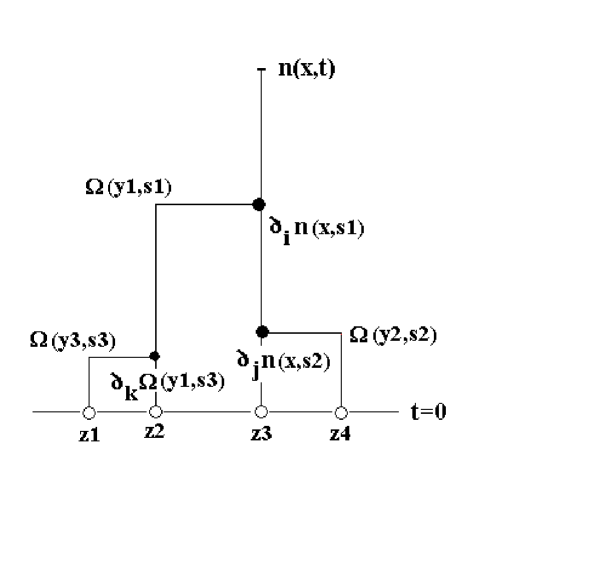
Figure 2: A sample path of the $n-$process

The contribution of this sample path to the $n-$expectation value is

$$M_{i,n}\left(x\right)M_{j,n}\left(x\right)\left\{\partial_{j}n_{0}\left(z_{3}\right)\partial_{i}\Omega_{0}\left(z_{4}\right)+\partial_{i}\partial_{j}n_{0}\left(z_{3}\right)\Omega_{0}\left(z_{4}\right)\right\}M_{k,\Omega}^{(a)}\left(y_{1}\right)\Omega_{0}\left(z_{1}\right)\partial_{k}\Omega_{0}\left(z_{2}\right)$$

Some remarks on this construction:

(i) The normalization of the kernels by the $h\left(x\right)$ function converts the computation of the integral into a probabilistic sampling. At the same time the kernel itself absorbs one of the derivatives, that otherwise would act on the fields.

(ii) The exponential $e^{-\phi}$ was expanded into a power series leading to multiple branchings with probabilities $p_{j,n}$ and $p_{j,\Omega}$. By contrast the other nonpolynomial term $\log n$ was kept as an operator. The reason is that the coefficients in the series expansion of the $\log$ do not lead to a probability distribution.

(iii) The complexity of the resulting processes, reflects the complexity of the original equations (20). Nevertheless what this construction shows is that clearly defined techniques may be used to construct stochastic solutions even when derivatives and complex non-linear terms are present.

To insure convergence of the calculation of the solution by the stochastic processes, a bound $M$ must be put on the multipliers (which depend on the normalization factors, hence on the $h\left(x\right)$ function), on the initial conditions $n_{0}\left(x\right)$ and $\Omega_{0}\left(x\right)$ and their derivatives, on the source term $S$ and on $\frac{\sigma\left(1-e^{\Lambda}\right)}{h\left(x\right)}$. From the branching process one estimates the probability of a tree of $n$ branches, therefore

$$M\leq\frac{1}{1-e^{-\sigma e^{\Lambda}t}}$$

3.2 The Fourier-transformed TOKAM 2D

In the Fourier transformed equation, the derivatives become simpler multiplicative factors. However the nonlinear terms become more complex. Let

$$f=\log n$$

Then, the first equation in (20) becomes

$$\frac{\partial}{\partial t}f=S^{\prime}-\{\phi,f\}-\sigma e^{\Lambda-\phi}+D\Delta_{\bot}f+D\left|\nabla f\right|^{2}$$ (32)

where the source term has been redefined as $S^{\prime}=\frac{S}{n}$. Let the Fourier transforms of $f$ and $\phi$ be

$$F\left(k,t\right) = \frac{1}{2\pi}\int d^{2}xf\left(x,t\right)e^{ik\cdot x}$$

$$\Phi\left(k,t\right) = \frac{1}{2\pi}\int d^{2}x\phi\left(x,t\right)e^{ik\cdot x}$$

Then, the Fourier transform of the equations (20) is

$$\frac{\partial}{\partial t}F\left(k,t\right) = -D\left|k\right|^{2}F\left(k,t\right)+\overset{\backsim}{S^{\prime}}\left(k,t\right)+\frac{1}{2\pi}\int d^{2}\xi\left(k_{1}-\xi_{1}\right)\xi_{2}\left\{\Phi\left(k-\xi\right)F\left(\xi\right)\right.$$

$$\left.-F\left(k-\xi\right)\Phi\left(\xi\right)\right\}$$

$$-\sigma e^{\Lambda}\sum_{n=0}^{\infty}\frac{\left(-1\right)^{n}}{n!\left(2\pi\right)^{n-1}}\Phi^{\ast n}\left(k\right)-\frac{D}{2\pi}\int d^{2}\xi\left\{\left(k_{1}-\xi_{1}\right)\xi_{1}\right.$$

$$+\left.\left(k_{2}-\xi_{2}\right)\xi_{2}\right\}F\left(k-\xi\right)F\left(\xi\right)$$

$$\frac{\partial}{\partial t}\Phi\left(k,t\right) = -\nu\left|k\right|^{2}\Phi\left(k,t\right)+\frac{1}{2\pi}\int\frac{d^{2}\xi}{\left|k\right|^{2}}\left(k_{1}-\xi_{1}\right)\xi_{2}\Phi\left(k-\xi\right)\Phi\left(\xi\right)\left\{\left|\xi\right|^{2}-\left|k-\xi\right|^{2}\right\}$$ (33)

$$-ig\frac{k_{2}}{\left|k\right|^{2}}F\left(k\right)-\frac{\sigma}{\left|k\right|^{2}}\left\{2\pi\delta^{2}\left(k\right)-e^{\Lambda}\sum_{n=0}^{\infty}\frac{\left(-1\right)^{n}}{n!\left(2\pi\right)^{n-1}}\Phi^{\ast n}\left(k\right)\right\}$$

where $\overset{\backsim}{S^{\prime}}$ is the Fourier transform of $S^{\prime}$ and $\Phi^{\ast n}$ denotes the convolution power.

$$\Phi^{\ast n}\left(k\right)=\int\prod_{i=1}^{n}d^{2}\xi^{(i)}\delta\left(k-\sum_{l=1}^{n}\xi^{(l)}\right)\prod_{p=1}^{n}\Phi\left(\xi^{(p)}\right)$$

To control the growth of the functional obtained by the stochastic process one divides $F\left(k,t\right)$ and $\Phi\left(k,t\right)$ by a majorizing kernel $\gamma\left(k\right)$

$$\chi\left(k,t\right) = \frac{F\left(k,t\right)}{\gamma\left(k\right)}$$

$$\zeta\left(k,t\right) = \frac{\Phi\left(k,t\right)}{\gamma\left(k\right)}$$ (34)

and writes integral equations for $\chi\left(k,t\right)$

$$\chi\left(k,t\right) = e^{-D\left|k\right|^{2}t}\chi\left(k,0\right)+\int_{0}^{t}dsD\left|k\right|^{2}e^{-D\left|k\right|^{2}s}\left\{p_{a}\int d^{2}\xi M_{a}\left(k,\xi\right)p\left(k,\xi\right)\right.$$ (35)

$$\left[\frac{1}{2}\zeta\left(k-\xi,t-s\right)\chi\left(\xi,t-s\right)-\frac{1}{2}\chi\left(k-\xi,t-s\right)\zeta\left(\xi,t-s\right)\right]$$

$$+p_{b}\sum_{n=0}p_{n}\int d^{2}\xi_{1}\cdots d^{2}\xi_{n-1}M_{n}\left(k,\xi_{1},\cdots,\xi_{n-1}\right)p\left(k,\xi_{1},\cdots,\xi_{n-1}\right)$$

$$\times\zeta\left(k-\sum_{i=1}^{n-1}\xi_{i},t-s\right)\zeta\left(\xi_{1},t-s\right)\cdots\zeta\left(\xi_{n-1},t-s\right)$$

$$+p_{c}\int d^{2}\xi p\left(k,\xi\right)\left[\frac{1}{2}M_{c}^{(1)}\left(k,\xi\right)+\frac{1}{2}M_{c}^{(2)}\left(k,\xi\right)\right]\chi\left(k-\xi,t-s\right)\chi\left(\xi,t-s\right)$$

$$\left.+p_{s}M_{s}\left(k\right)\frac{\overset{\backsim}{S^{\prime}}\left(k,t-s\right)}{\gamma\left(k\right)}\right\}$$

with probabilities

$$p_{a} = \left(1+D+2\pi+2\pi\sigma e^{\Lambda}\right)^{-1}$$

$$p_{b} = 2\pi\sigma e^{\Lambda+1}\left(1+D+2\pi+2\pi\sigma e^{\Lambda}\right)^{-1}$$

$$p_{c} = D\left(1+D+2\pi+2\pi\sigma e^{\Lambda}\right)^{-1}$$

$$p_{s} = 2\pi\left(1+D+2\pi+2\pi\sigma e^{\Lambda}\right)^{-1}$$

$$p_{n} = \left(en!\right)^{-1}$$

$$p\left(k,\xi_{1},\cdots,\xi_{n-1}\right) = \frac{\gamma\left(k-\sum_{i=1}^{n-1}\xi_{i}\right)\gamma\left(\xi_{1}\right)\cdots\gamma\left(\xi_{n-1}\right)}{\gamma^{\ast n}\left(k\right)}$$ (36)

and multipliers

$$M_{a}\left(k,\xi\right) = \frac{\left(k_{1}-\xi_{1}\right)\xi_{2}\gamma\ast\gamma\left(k\right)}{\gamma\left(k\right)D\left|k\right|^{2}\pi}\left(1+D+2\pi+2\pi\sigma e^{\Lambda}\right)$$

$$M_{c}^{(1)}\left(k,\xi\right) = -\frac{\left(k_{1}-\xi_{1}\right)\xi_{1}\gamma\ast\gamma\left(k\right)}{\gamma\left(k^{2}\right)\left|k\right|^{2}\pi}\left(1+D+2\pi+2\pi\sigma e^{\Lambda}\right)$$

$$M_{c}^{(2)}\left(k,\xi\right) = -\frac{\left(k_{2}-\xi_{2}\right)\xi_{2}\gamma\ast\gamma\left(k\right)}{\gamma\left(k^{2}\right)D\left|k\right|^{2}\pi}\left(1+D+2\pi+2\pi\sigma e^{\Lambda}\right)$$

$$M_{n}\left(k\right) = -\frac{\left(-1\right)^{n}e\gamma^{\ast n}\left(k\right)}{\left(2\pi\right)^{n}\gamma\left(k\right)D\left|k\right|^{2}}\left(1+D+2\pi+2\pi\sigma e^{\Lambda}\right)$$

$$M_{s}\left(k\right) = \frac{1}{2\pi D\left|k\right|^{2}}\left(1+D+2\pi+2\pi\sigma e^{\Lambda}\right)$$ (37)

Notice that the term $n=0$ in the sum is $p_{b}p_{0}M_{0}\delta\left(k^{2}\right)$ which, when chosen, kills the contribution of the corresponding sample path for $k\neq 0$.

For $\varsigma\left(k,t\right)$

$$\zeta\left(k,t\right) = e^{-\nu\left|k\right|^{2}t}\zeta\left(k,0\right)+\int_{0}^{t}ds\nu\left|k\right|^{2}e^{-\nu\left|k\right|^{2}s}\left\{p_{a}^{\prime}\int d^{2}\xi M_{a}^{\prime}\left(k,\xi\right)p\left(k,\xi\right)\right.$$ (38)

$$\times\zeta\left(k-\xi,t-s\right)\zeta\left(\xi,t-s\right)+p_{b}^{\prime}\sum p_{n}\int d^{2}\xi_{1}\cdots d^{2}\xi_{n-1}M_{n}^{\prime}\left(k,\xi_{1},\cdots,\xi_{n-1}\right)$$

$$\times p\left(k,\xi_{1},\cdots,\xi_{n-1}\right)\zeta\left(k-\sum_{i=1}^{n-1}\xi_{i},t-s\right)\cdots\zeta\left(\xi_{n-1},t-s\right)$$

$$\left.+p_{\chi}M_{\chi}\left(k,\xi\right)\chi\left(k,t-s\right)\right\}$$

with probabilities and multipliers

$$p_{a}^{\prime} = \left(\frac{1}{2\pi}+g+\sigma\right)^{-1}\frac{1}{2\pi}$$

$$p_{b}^{\prime} = \left(\frac{1}{2\pi}+g+\sigma\right)^{-1}\sigma$$

$$p_{\chi} = \left(\frac{1}{2\pi}+g+\sigma\right)^{-1}g$$

$$p_{n} = \left(en!\right)^{-1}$$

$$p\left(k,\xi_{1},\cdots,\xi_{n-1}\right) = \frac{\gamma\left(k-\sum_{i=1}^{n-1}\xi_{i}\right)\gamma\left(\xi_{1}\right)\cdots\gamma\left(\xi_{n-1}\right)}{\gamma^{\ast n}\left(k\right)}$$ (39)

$$M_{a}^{\prime}\left(k,\xi\right) = \frac{\left(k_{1}-\xi_{1}\right)\xi_{2}\left\{\left|\xi\right|^{2}-\left|k-\xi\right|^{2}\right\}\gamma\ast\gamma\left(k\right)}{\gamma\left(k\right)\nu\left|k\right|^{4}}\left(\frac{1}{2\pi}+g+\sigma\right)$$

$$M_{n}\left(k\right) = \frac{\left(-1\right)^{n}e^{\Lambda}\gamma^{\ast n}\left(k\right)}{\left(2\pi\right)^{n-1}\gamma\left(k\right)\nu\left|k\right|^{4}}\left(\frac{1}{2\pi}+g+\sigma\right)\hskip 14.22636ptn\geq 1$$

$$M_{0}\left(k\right) = \frac{2\pi\left(e^{\Lambda}-1\right)}{\gamma\left(k\right)\nu\left|k\right|^{4}}\left(\frac{1}{2\pi}+g+\sigma\right)$$

$$M_{\chi}\left(k\right) = \frac{-ik_{2}}{\nu\left|k\right|^{4}}\left(\frac{1}{2\pi}+g+\sigma\right)$$ (40)

The probabilistic interpretation of these equations is similar to the previous cases. There are two stochastic processes that started at $t$, propagate backwards in time as Brownian motions with coefficients $D\left|k\right|^{2}$ and $\nu\left|k\right|^{2}$. With probabilities $e^{-D\left|k\right|^{2}t}$ or $e^{-\nu\left|k\right|^{2}t}$ the processes either reach $t=0$ without branching or branch with probability densities $D\left|k\right|^{2}e^{-D\left|k\right|^{2}s}$ or $\nu\left|k\right|^{2}e^{-\nu\left|k\right|^{2}s}$ at time $t-s$. The branch that they follow afterwards is controlled by the probabilities in (36) and (39). Because products become convolutions under the Fourier transform, probability densities are needed to decide the new momenta of the branches. The main role of the majorizing kernel $\gamma\left(k\right)$ is to normalize these probability densities in momentum space. At each branching point the process picks up the multipliers in (37) and (40), the contribution of each sample path to the the expectation values of $\chi\left(k,t\right)$ and $\zeta\left(k,t\right)$ being the initial values of the corresponding fields $\chi\left(k,0\right)$ or $\zeta\left(k,0\right)$ when the processes reach time zero multiplied by the multipliers picked up along the path. In this case because there are no operator labels, there is no need to backtrack forward in time as in the configuration space equation. The price one pays is a more complex branching structure at each vertex.

A strict condition for the convergence of the process is obtained by a bound $M\leq 1$ on all the factors that intervene in the final calculation of each path contribution.

4 Remarks and conclusions

1) The scrape-off layer equations provide a good testing ground for the construction of stochastic solutions when the equations contain nonpolynomial terms and derivatives. Therefore, the techniques developed here considerably extend the range of equations to which the stochastic solution technique may be applied.

2) To obtain good accuracy in the stochastic solutions, many sample paths should be computed for each starting configuration. How many samples are needed may be estimated by large deviation techniques [23]. The sample independence character of the stochastic calculation reduces the severity of this problem when using parallel computing. Nevertheless it should be pointed out that, when solutions are desired over a large domain, the stochastic method is computationally competitive only when applied together with the domain decomposition method [17] [18] [19]. Then a considerable improvement is obtained. However, if local solutions on configuration or Fourier space are desired, the stochastic method is quite appropriate. For example a study of the time evolution of a few high Fourier modes gives information on the turbulence spectrum that only a very fine grid and an expensive calculation would provide with a global deterministic algorithm.

References

• [1] R. M. Blumenthal and R. K. Getoor; Markov processes and potential theory, Academic Press, New York 1968.
• [2] R. F. Bass; Probabilistic techniques in analysis, Springer, New York 1995.
• [3] R. F. Bass; Diffusions and elliptic operators, Springer, New York 1998.
• [4] H. P. McKean; Comm. on Pure and Appl. Math. 28 (1975) 323-331, 29 (1976) 553-554.
• [5] E. B. Dynkin; Diffusions, Superdiffusions and Partial Differential Equations, AMS Colloquium Pubs., Providence 2002.
• [6] E. B.Dynkin; Superdiffusions and positive solutions of nonlinear partial differential equations, AMS , Providence.2004.
• [7] Y. LeJan and A. S. Sznitman ; Prob. Theory and Relat. Fields 109 (1997) 343-366.
• [8] E. C. Waymire; Prob. Surveys 2 (2005) 1-32.
• [9] R. N. Bhattacharya et al. ; Trans. Amer. Math. Soc. 355 (2003) 5003-5040
• [10] M. Ossiander ; Prob. Theory and Relat. Fields 133 (2005) 267-298.
• [11] J. C. Orum; Stochastic cascades and 2D Fourier Navier-Stokes equations, in Lectures on multiscale and multiplicative processes, www.maphysto.dk/publications/MPS-LN/2002/11.pdf
• [12] R. Vilela Mendes and F. Cipriano; Commun. Nonlinear Science and Num. Simul. 13 (2008) 221-226 and 1736.
• [13] E. Floriani, R. Lima and R. Vilela Mendes; European Physical Journal D 46 (2008) 295-302 and 407.
• [14] R. Vilela Mendes; Stochastics 81 (2009) 279-297.
• [15] R. Vilela Mendes; J. Math. Phys. 51 (2010) 043101.
• [16] F. Cipriano, H. Ouerdiane and R. Vilela Mendes; Fract. Calc. Appl. Anal.Β 12 (2009) 47-56.
• [17] J. A. AcebrΓ³n, A. Rodriguez-Rozas and R. Spigler; J. of Computational Physics 228 (2009) 5574–5591.
• [18] J.A. AcebrΓ³n, A. RodrΓ­guez-Rozas and R. Spigler; J. on Scientific Computing 43 (2010) 135-157.
• [19] J.A. AcebrΓ³n and A. RodrΓ­guez-Rozas; J. of Computational Physics 230 (2011) 7891–7909.
• [20] R. Vilela Mendes; Stochastic solutions of nonlinear PDE’s: McKean versus superprocesses, arXiv:1111.5504, in Proceedings of ”Chaos, Complexity and Transport”, X. Leoncini (Ed.) World Scientific 2012.
• [21] H. Bufferand, G. Ciraiolo, L. Isoardi, G. Chiavassa, F. Schwander, E. Serre, N. Fedorczak, Ph. Ghendrih and P. Tamain; J. Nucl. Materials (2010) doi:10.1016/j.jnucmat.2010.11.037
• [22] Y. Sarazin; Ph. Ghendrih; Phys. Plasmas 5 (1998) 4214.
• [23] E. Floriani and R. Vilela Mendes; A stochastic approach to the solution of magnetohydrodynamic equations, arXiv:1112.2166