Modeling of the magnetic properties of nanomaterials with different crystalline structure
Abstract
We propose a method for modeling the magnetic properties of nanomaterials with different structures. The method is based on the Ising model and the approximation of the random field interaction. It is shown that in this approximation, the magnetization of the nanocrystal depends only on the number of nearest neighbors of the lattice atoms and the values of exchange integrals between them. This gives a good algorithmic problem of calculating the magnetization of any nano-object, whether it is ultrathin film or nanoparticle of any shape and structure, managing only a rule of selection of nearest neighbors. By setting different values of exchange integrals, it is easy to describe ferromagnets, antiferromagnets, and ferrimagnets in a unified formalism. Having obtained the magnetization curve of the sample it is possible to find the Curie temperature as a function of, for example, the thickness of ultrathin film. Afterwards one can obtain the numerical values for critical exponents of the phase transition “ferromagnet – paramagnet”. Good agreement between the results of calculations and the experimental data proves the correctness of the method.
1 Introduction
Creation of magnetic materials with predetermined properties – the task of unquestionable importance. While the manipulation of individual atoms becomes a routine, nanotechnologies need appropriate calculation methods, which would allow prototyping magnetic properties of materials without heavy calculations on supercomputers. The method proposed below satisfies such requirements. Moreover, it allows calculus of the properties of magnets of any type (ferromagnets, antiferromagnets, ferrimagnets) to be provided using a uniform formalism.
Another feature of nano-objects is the existence of size effects at their scale. Obviously, such effects are different in two-dimensional films and three-dimensional particles. Furthermore, it is common to use different methods of modeling for nanoparticles of different shape. But if to consider the theory with short-range interaction, the global geometry of the material should not play any role. In this case, there must be a simulation method that is insensitive to the shape of the simulated sample as a whole. We offer in this paper such a method.
2 General model of magnetic material
We assume that magnetic atoms are distributed over sites of the sample with probability . According to [1], the distribution function for random interaction fields on a particle located at the origin can be defined as:
| (1) |
where – Dirac delta function, – field created by atoms with magnetic moments located at coordinates , – the coordinates of lattice sites, – the distribution function for the magnetic moments, which in the approximation of Ising model for a ferromagnets can be represented as follows:
| (2) |
Here – the angle between and -axis, and – relative probabilities of the spin orientation along and against -axis ( and , respectively); – magnitude of magnetic moment of a magnetic atom. Probabilities and hold normalization condition . In the approximation of nearest neighbors and the direct exchange interaction between magnetic atoms, the equation (1) can be represented as:
| (3) |
where is a set of nearest neighbors of the magnetic atom numbered as , – its coordination number; – subset of atoms of the total number of nearest neighbors of atom; is a binomial set of permutations of an arbitrary set with the amount of elements equal to . Introducing symmetric notation we have got and . Finally, is the constant of exchange interaction (exchange integral).
Using the expression for the distribution function of interaction fields (3), one can obtain equations that determine average relative magnetic moments at each site of lattice:
| (4) |
Expression (4) allows to investigate the dependence of total magnetic moment of the sample at the temperature and concentration , as well as to determine the dependence on the number of atoms of the temperature of phase transition and the percolation threshold. System of equations with unknowns (4) can be solved numerically using Newton’s method111 In our research we use Wolfram Mathematica for fast lattice prototyping and C++ and Fortran non-linear solvers with python wrapper for precise calculus..
3 Modeling of magnetic materials with different crystalline structure
Equation (4), despite the complicated form, has written in the algorithmically convenient form. This form allows to simulate the magnetic properties of materials, based only on the knowledge of the crystalline structure of the sample and the numerical values of the exchange integrals.
Crucial part of this method is the rule of selection of nearest neighbors for each atom (the way of constructing of the set ). By changing this rule of selection we can easily adjust our model to different physical systems. We also can simulate antiferromagnetic and ferrimagnetic materials by reversing signs and values of exchange integrals of individual atoms.
Consider two examples of applying the method described above.
3.1 Ultrafine particles
Consider a nanoparticle of atoms. Then (4) is a system of independent equations with unknowns. In some cases, when , the symmetry of the particle reduces the number of unknowns, but in general all variables are different.
For example, for cubic-shaped nanoprticle with atoms on the edge and simple cubic lattice there is a system of non-algebraic equations with unknowns. Even relatively small cubic particle with atoms on the edge contains atoms, which makes calculation non-trivial and significantly reduces its accuracy.
3.2 Thin films
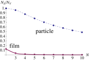
Now consider ultrathin film that is composed of infinite monolayers. In a simple case when all atoms from the same layer are equal, (4) turns into a system of equations with unknowns. Study of size effects in films is much easier than in the particles, because it is sufficient to simulate a film of 10-15 layers to achieve the bulk properties. (See fig. 1.)
General equation that determines the average relative magnetic moment in -th monolayer is given by (4). Replacing in expressions for and all on their average values and substituting (3) into (4), one can obtain the equations that determine in each monolayer:
| (5) |
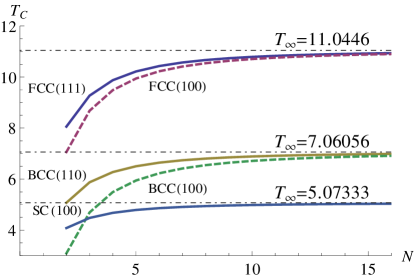
where is the number of nearest neighbors in the -th layer, is the number of nearest neighbors of the atom in -th layer, located in the -th layer; , , , . Using (5), one can study the dependence of the average magnetic moment of the film on its temperature and thickness [2], and, as a consequence, the dependence of Curie temperature on the thickness (see fig. 2).
4 Comparison with experimental data
Comparison of the results of modeling with experimental data was carried out directly and indirectly.
4.1 Direct comparison: relative Curie temperature change
4.2 Indirect comparison: critical exponents
It is possible to obtain the value of critical exponent of spin-spin correlation for phase transition “ferromagnet – paramagnet” by appropriate approximation of defined above. Critical exponents for ultrathin films of different crystalline structures were obtained in [2]. It was shown that the value of for three-dimensional Ising model is independent from the type of the lattice. The numerical value of is close to the value obtained from RG-calculations [5].
5 Conclusion
Offered method of simulating allows to substitute the real magnetic material with the relatively simple model, where the key role is played by the coordination number and the exchange integrals. All the magnetic geometry lies in these two integral characteristics. By setting only the rules of choice of nearest neighbors and values of corresponding exchange integrals, we make the modeling procedure very effective.
The work was supported by grant of Scientific Fund of Far Eastern Federal University (FEFU) \No 12-07-13000-FEFU_a.
References
References
- [1] Belokon V and Nefedev K 2001 Journal of Experimental and Theoretical Physics 93(1) 136–142 ISSN 1063-7761 10.1134/1.1391530 URL http://dx.doi.org/10.1134/1.1391530
- [2] Afremov L and Kirienko Y 2012 Advanced Materials Research 378–379 589–592 (Preprint http://arxiv.org/abs/1108.0745)
- [3] Kirienko Y and Afremov L 2012 Advanced Materials Research 472–473 1827–1830 (Preprint http://arxiv.org/abs/1201.1562)
- [4] Sadeh B, Doi M, Shimizu T and Matsui M 2000 Journal of the Magnetics Society of Japan 24 511–514
- [5] Le Guillou J and Zinn-Justin J 1977 Phys. Rev. Lett. 39 95–98