Cramér-Rao-Induced Bounds for CANDECOMP/PARAFAC tensor decomposition

Abstract

This paper presents a Cramér-Rao lower bound (CRLB) on the variance of unbiased estimates of factor matrices in Canonical Polyadic (CP) or CANDECOMP/PARAFAC (CP) decompositions of a tensor from noisy observations, (i.e., the tensor plus a random Gaussian i.i.d. tensor). A novel expression is derived for a bound on the mean square angular error of factors along a selected dimension of a tensor of an arbitrary dimension. The expression needs less operations for computing the bound, $O(NR^{6})$, than the best existing state-of-the art algorithm, $O(N^{3}R^{6})$ operations, where $N$ and $R$ are the tensor order and the tensor rank. Insightful expressions are derived for tensors of rank 1 and rank 2 of arbitrary dimension and for tensors of arbitrary dimension and rank, where two factor matrices have orthogonal columns.

The results can be used as a gauge of performance of different approximate CP decomposition algorithms, prediction of their accuracy, and for checking stability of a given decomposition of a tensor (condition whether the CRLB is finite or not). A novel expression is derived for a Hessian matrix needed in popular damped Gauss-Newton method for solving the CP decomposition of tensors with missing elements. Beside computing the CRLB for these tensors the expression may serve for design of damped Gauss-Newton algorithm for the decomposition.

Index Terms

Multilinear models; canonical polyadic decomposition; Cramér-Rao lower bound; stability; uniqueness

I Introduction

Order-3 and higher-order data arrays need to be analyzed in diverse research areas such as chemistry, astronomy, and psychology [1]–[3]. The analyses can be done through finding multi-linear dependencies among elements within the arrays. The most popular model is Parallel factor analysis (PARAFAC), also called Canonical decomposition (CANDECOMP) or CP, which is an extension of a low rank decomposition of matrices to higher-way arrays, usually called tensors. In signal processing, the tensor decompositions have become popular for their usefulness in blind source separation [4].

Note that a best-fitting CP decomposition may not exist for some tensors. In that case, trying to find a best-fitting CP decomposition results in diverging factors [5, 6]. This paper is focussed on studying CP decompositions of a noisy observations of tensors, which admit an exact CP decomposition. The decomposition of the noiseless tensor is taken as a ground truth for computing errors.

An important issue is the essential uniqueness of CP decomposition as it entails identifiability of the model (the factor matrices) from the tensor. The adjective “essential” means that the model is unique up to a scale and permutation ambiguity, which is inherent to the problem. Initial works in the field can be traced back in 70’s in works of Harshman [7, 8]. A popular sufficient condition for the uniqueness was derived by Kruskal in [9]. Recently, the problem has been addressed again, namely by Stegeman, Ten Berge, De Lathauwer, Jiang, Sidiropoulos et al.; see [10]-[22].

This paper is focussed on stability of the CP decomposition rather than on the uniqueness. By stability we mean existence of a finite Cramér-Rao bound in a stochastic set-up, where tensor elements are corrupted by additive Gaussian-distributed noise. Relation of this kind of stability to a deterministic stability and to the uniqueness was studied in [23]. It is not true, in general, that stability of a solution of a nonlinear problem implies uniqueness of the solution. For example, there might always be a permutation or sign ambiguity. It is yet an open theoretical question if stability of the CP tensor decomposition problem implies its essential uniqueness. Regardless of the missing link to identifiability, the stability is an interesting concept which is worth to be studied, because different kind of noise is very common.

In general, in order to evaluate performance of a tensor decomposition, the approximation error between the data tensor and its approximate is commonly used. Unfortunately, such measure does not imply quality of the estimated components. In practice, in some difficult scenarios such as decomposition of tensor with linear dependency among components of factor matrices, or large difference in magnitude between components [24, 25], most CP algorithms explained the data tensor at almost identical fit, but only few algorithms can accurately retrieve the hidden components from the tensor [26, 24]. In order to verify theoretically the quality of the estimated components and evaluate robustness of an algorithm, an appropriate measure is an essential prerequisite. The squared angular error between the estimated component and its original one is such a measure [27, 28]. Working with angular errors is practical, because the scaling ambiguity does not play a role. Only the permutation ambiguity has to be solved in practical examples, because order of the factor can be quite arbitrary.

Cramér-Rao lower bound for CP decomposition was first studied in [29], and later, a more compact asymptotic expression was derived in [30] for tensors of order 3 appearing in wireless communications. A non-asymptotic (exact) CRLB-induced bound (CRIB) on squared angular deviation of columns of the factor matrices with respect to their nominal values has been studied in [27]. Similar results for symmetric tensors are derived in [31]. Nevertheless, the study is limited to the case of three-way tensors. In the general case, CRIB can be, indeed, calculated through the approximate Hessian which is often huge, and is impractical to directly invert. Note that such task normally costs $O(R^{3}T^{3})$ where $T=\sum_{n}I_{n}$. Seeking a cheaper method for CRIB is a challenge to made it applicable.

This paper presents new CRIB expressions for tensors of arbitrary dimension and rank, and specialized expressions for rank 1 and rank 2 tensors. The results rely on compact expressions for Hessian of the problem derived in [26]. Alternative expressions for the Hessian exist in [37]. Note, however, that unlike [26], this paper presents different expressions for inverse of the Hessian, which have lower computational complexity. In particular, complexity of inversion of the Hessian is reduced from $O(N^{3}R^{6})$ operations to $O(NR^{6})$, where $N$ and $R$ are the tensor order and the tensor rank, respectively.

On basis of new discovered properties of the CRIB, we established connection between theoretical and practical results in CPD:

• Stability of CPD for rank-1 and rank-2 tensors of arbitrary dimension.

• The work may serve as theoretical support for a novel CP decomposition algorithm through tensor reshaping [32], which was designed to decompose high-dimensional and high-order tensors. In particular, it appears that higher-order orthogonally constrained CPD [33, 34, 35, 36] can be decomposed efficiently through tensor unfolding.

• Stability when factor matrices occur linear dependence problem and especially the rank-overlap problem [1, 22, 34]. The problem is related to a variant of CPD for linear dependent loadings which was investigated in chemometric data and in flow injection analysis [1, 34]. A partial uniqueness condition of the related model is discussed in [22].

• CP decomposition of tensors with missing entries, which is quite frequent in practice, is addressed. An approximate Hessian for this case is derived, which is the core for the damped Gauss-Newton algorithm for the decomposition.

• A maximum tensor rank, given dimension of the tensor, which admits a stable decomposition is discussed.

The paper is organized as follows. Section II presents the main result, the Cramér-Rao induced bound on angular error of one factor vector in full generality. In Section III, this result is specialized for tensors of rank 1 and rank 2, and for the case when two factor matrices have mutually orthogonal columns. Section IV is devoted to a possible application of the bound: investigation of loss of accuracy of the tensor decomposition when the tensor is reshaped to a lower-dimensional form. Section V deals with the bound for tensors with missing entries, Section VI contains examples – CRIB computed for CP decomposition of a fluorescence tensor, stability of the tensor investigated by Brie et al, and a discussion of a maximum stable rank given the tensor dimension. Section VII concludes the paper.

II Presentation of the CRIB

II-A Cramér-Rao bound for CP decomposition

Let $\boldsymbol{\mathscr{{Y}}}$ be an $N-$ way tensor of dimension $I_{1}\times I_{2}\times\ldots\times I_{N}$. The tensor is said to be of rank $R$, if $R$ is the smallest number of rank-one tensors which admit the decomposition of $\boldsymbol{\mathscr{{Y}}}$ of the form

$$\boldsymbol{\mathscr{{Y}}}=\sum\limits_{r=1}^{R}{{\bf a}^{(1)}_{r}\circ{\bf a}^{(2)}_{r}\circ\ldots\circ{\bf a}^{(N)}_{r}}$$ (1)

where $\circ$ denotes the outer vector product, ${\bf a}^{(n)}_{r}$, $r=1,\ldots,R$, $n=1,\ldots,N$ are vectors of the length $I_{n}$ called factors. The tensor in (1) can be characterized by $N$ factor matrices ${\bf A}_{n}=[{\bf a}^{(n)}_{1},{\bf a}^{(n)}_{2},\ldots,{\bf a}^{(n)}_{R}]$ of the size $I_{n}\times R$ for $n=1,\ldots,N$. Sometimes (1) is referred to as a Kruskal form of a tensor [43].

In practice, CP decomposition of a given rank ($R$) is used as an approximation of a given tensor, which can be a noisy observation ${\hat{\boldsymbol{\mathscr{{Y}}}}}$ of the tensor $\boldsymbol{\mathscr{{Y}}}$ in (1). Owing to the symmetry of (1), we can focus on estimating the first factor matrix ${\bf A}_{1}$, without any loss of generality, and we can assume that all other factor matrices have columns of unit norm. Then the “energy” of the parallel factors is determined by the squared Euclidean norm of columns of ${\bf A}_{1}$.

It is common to assume that the noise has a zero mean Gaussian distribution with variance $\sigma^{2}$, and is independently added to each element of the tensor in (1).

Let a vector parameter $\theta$ containing all parameters of our model be arranged as

$$\mbox{\boldmath{$\theta$}}=[({\tt vec}\,{\bf A}_{1})^{T},\ldots,({\tt vec}\,{\bf A}_{N})^{T}]^{T}~{}.$$ (2)

The maximum likelihood solution for $\theta$ consists in minimizing the least squares criterion

$${\cal Q}(\mbox{\boldmath{$\theta$}})=\|{\hat{\boldsymbol{\mathscr{{Y}}}}}-\boldsymbol{\mathscr{{Y}}}(\mbox{\boldmath{$\theta$}})\|_{F}^{2}$$ (3)

where $\|\cdot\|_{F}$ stands for the Frobenius norm.

We wish to compute the Cramér-Rao lower bound for estimating $\theta$. In general, for this estimation problem, the CRLB is given as the inverse of the Fisher information matrix, which is equal to [27]

$${\bf F}(\mbox{\boldmath{$\theta$}})=\frac{1}{\sigma^{2}}\,{\bf J}^{T}(\mbox{\boldmath{$\theta$}}){\bf J}(\mbox{\boldmath{$\theta$}})$$ (4)

where ${\bf J}(\mbox{\boldmath{$\theta$}})$ is the Jacobi matrix (matrix of the first-order derivatives) of ${\cal Q}(\mbox{\boldmath{$\theta$}})$ with respect to $\theta$. In other words, the Fisher information matrix is proportional to the approximate Hessian matrix of the criterion, ${\bf H}(\mbox{\boldmath{$\theta$}})={\bf J}^{T}(\mbox{\boldmath{$\theta$}}){\bf J}(\mbox{\boldmath{$\theta$}})$.

Let $\boldsymbol{\Gamma}_{nm}$ denote the Hadamard (elementwise) product of matrices ${\bf C}_{k}={\bf A}_{k}^{T}{\bf A}_{k},k\in\{1,\ldots,N\}-\{n,m\}$,

$${\mbox{\boldmath$\Gamma$}}_{nm} = \mathop{\mbox{$\circledast$}}\limits_{k\neq n,m}{{\bf C}_{k}}\,,\qquad{\bf C}_{k}={\bf A}_{k}^{T}{\bf A}_{k}~{}.$$ (5)

Theorem 1 [26]: The Hessian ${\bf H}$ can be decomposed into low rank matrices under the form as

$${\bf H}={\bf G}+{\bf Z}\,{\bf K}\,{\bf Z}^{T}$$ (6)

where ${\bf K}=\left[{\bf K}_{nm}\right]_{n,m=1}^{N}$ contains submatrices ${\bf K}_{nm}$ given by

$${\bf K}_{nm}=(1-\delta_{nm}){\bf P}_{R}\,\operatorname{dvec}\,(\mbox{\boldmath$\Gamma$}_{nm})$$ (7)

${\bf P}_{R}$ is the permutation matrix of dimension $R^{2}\times R^{2}$ defined in [26] such that ${\tt{vec}}\,{{\bf M}}={\bf P}_{R}\,{\tt{vec}}\,({{\bf M}^{T}})$ for any $R\times R$ matrix ${\bf M}$, and $\delta_{nm}$ is the Kronecker delta, and ${\tt dvec}({\bf M})$ is a short-hand notation for ${\tt diag}({\tt vec}({\bf M}))$, i.e. a diagonal matrix containing all elements of a matrix ${\bf M}$ on its main diagonal. Next,

$${\bf G} = {\tt{bdiag}}\left({\boldsymbol{\Gamma}}_{nn}\otimes{\bf I}_{I_{n}}\right)_{n=1}^{N}$$ (8)

and

$${\bf Z}={\tt{bdiag}}\left({\bf I}_{R}\otimes{\bf A}_{n}\right)_{n=1}^{N}$$ (9)

where $\otimes$ denotes the Kronecker product, ${\bf I}_{I_{n}}$ is an identity matrix of the size $I_{n}\times I_{n}$, and ${\tt{bdiag}}(\cdot)$ is a block diagonal matrix with the given blocks on its diagonal. Note that the Hessian ${\bf H}$ in (6) is rank deficient because of the scale ambiguity of columns of factor matrices [25, 39]. It has dimension $\left(R\sum_{n}I_{n}\right)\times\left(R\sum_{n}I_{n}\right)$ but its rank is at most $R\sum_{n}I_{n}-(N-1)R$.

A regular (reduced) Hessian can be obtained from ${\bf H}$ by deleting $(N-1)R$ rows and corresponding columns in ${\bf H}$, because the estimation of one element in the vectors ${\bf a}_{r}^{(n)}$, $r=1,\ldots,R$, $n=2,\ldots,N$ can be skipped. The reduced Hessian may have the form

$${\bf H}_{E}={\bf E}{\bf H}{\bf E}^{T}$$ (10)

where

$${\bf E}={\tt{bdiag}}\left({\bf I}_{RI_{1}},{\bf I}_{R}\otimes{\bf E}_{2},\ldots,{\bf I}_{R}\otimes{\bf E}_{N}\right)$$ (11)

and ${\bf E}_{n}$ is an $(I_{n}-1)\times I_{n}$ matrix of rank $I_{n}-1$. For example, one can put ${\bf E}_{n}=[{\bf 0}_{(I_{n}-1)\times 1}\,{\bf I}_{I_{n}-1}]$ for $n=2,\ldots,N$. With this definition of ${\bf E}_{n}$, ${\bf H}_{E}$ is a Hessian for estimating the first factor matrix ${\bf A}_{1}$ and all other vectors ${\bf a}_{r}^{(n)}$, $r=1,\ldots,R$, $n=2,\ldots,N$ without their first elements. In the sequel, however, we use a different definition of ${\bf E}_{n}$. Note that each ${\bf E}_{n}$ can be quite arbitrary, together facilitate a regular transformation of nuisance parameters, which does not influence CRLB of the parameter of interest.

The CRLB for the first column of ${\bf A}_{1}$, denoted simply as ${\bf a}_{1}$, is defined as $\sigma^{2}$ times the left-upper submatrix of ${\bf H}_{E}^{-1}$ of the size $I_{1}\times I_{1}$,

$$\mbox{CRLB}({\bf a}_{1})=\sigma^{2}\,[{\bf H}_{E}^{-1}]_{1:I_{1},1:I_{1}}~{}.$$ (12)

Substituting (6) in (10) gives

$${\bf H}_{E}={\bf G}_{E}+{\bf Z}_{E}{\bf K}{\bf Z}_{E}^{T}$$ (13)

where ${\bf G}_{E}={\bf E}{\bf G}{\bf E}^{T}$ and ${\bf Z}_{E}={\bf E}{\bf Z}$. Inverse of ${\bf H}_{E}$ can be written using a Woodbury matrix identity [38] as

$${\bf H}_{E}^{-1}={\bf G}_{E}^{-1}-{\bf G}_{E}^{-1}{\bf Z}_{E}{\bf K}({\bf I}_{NR^{2}}+{\bf Z}_{E}^{T}{\bf G}_{E}^{-1}{\bf Z}_{E}{\bf K})^{-1}{\bf Z}_{E}^{T}{\bf G}_{E}^{-1}$$ (14)

provided that the involved inverses exist.

Next,

$${\bf G}_{E} = {\tt{bdiag}}\left({\boldsymbol{\Gamma}}_{11}\otimes{\bf I}_{1},{\boldsymbol{\Gamma}}_{22}\otimes({\bf E}_{2}{\bf E}_{2}^{T}),\ldots,{\boldsymbol{\Gamma}}_{NN}\otimes({\bf E}_{N}{\bf E}_{N}^{T})\right)$$ (15)

$${\bf G}_{E}^{-1} = {\tt{bdiag}}\left(({\boldsymbol{\Gamma}}_{11})^{-1}\otimes{\bf I}_{1},\mbox{\boldmath$\Gamma$}_{22}^{-1}\otimes({\bf E}_{2}{\bf E}_{2}^{T})^{-1},\ldots,{\boldsymbol{\Gamma}}_{NN}^{-1}\otimes({\bf E}_{N}{\bf E}_{N}^{T})^{-1}\right)~{}.$$ (16)

Put

$$\Psi = {\bf Z}_{E}^{T}{\bf G}_{E}^{-1}{\bf Z}_{E}$$ (17)

$${\bf B} = {\bf K}({\bf I}_{NR^{2}}+\mbox{\boldmath{$\Psi$}}{\bf K})^{-1}$$ (18)

and let ${\bf B}_{0}$ be the upper–left $R^{2}\times R^{2}$ submatrix of ${\bf B}$, symbolically ${\bf B}_{0}={\bf B}_{1:R^{2},1:R^{2}}$. Finally, let $g_{11}$ and ${\bf g}_{1,:}$ be the upper–left element and the first row of ${\boldsymbol{\Gamma}}_{11}^{-1}$, respectively. Then

$$[{\bf H}_{E}^{-1}]_{1:I_{1},1:I_{1}} = [{\bf G}_{E}^{-1}]_{1:I_{1},1:I_{1}}+[{\bf G}_{E}^{-1}{\bf Z}_{E}]_{1:I_{1},1:R^{2}}{\bf B}_{0}[{\bf G}_{E}^{-1}{\bf Z}_{E}]_{1:I_{1},1:R^{2}}^{T}$$ (19)

$$= g_{11}{\bf I}_{I_{1}}+\left({\bf g}_{1,:}\otimes{\bf A}_{1}\right){\bf B}_{0}\left({\bf g}_{1,:}\otimes{\bf A}_{1}\right)^{T}~{}.$$

The CRLB represents a lower bound on the error covariance matrix $\mbox{E}[(\hat{{\bf a}}_{1}-{\bf a}_{1})(\hat{{\bf a}}_{1}-{\bf a}_{1})^{T}]$ for any unbiased estimator of ${\bf a}_{1}$. The bound is asymptotically tight in the case of Gaussian noise and least squares estimator, which is equivalent to maximum likelihood estimator, under the assumptions that the permutation ambiguity has been solved out (order of the estimated factors was selected to match the original factors) and scaling of the estimator is in accord with the selection of the matrix ${\bf E}$.

II-B Cramér-Rao-induced bound for angular error

CRLB(${\bf a}_{1}$) considered in the previous subsection is a matrix. In applications it is practical to characterize the error of the factor ${\bf a}_{1}$ in the decomposition by a scalar quantity. In [28] it was proposed to characterize the error by an angle between the true and the estimated vector, and compute a Cramér-Rao-induced bound (CRIB) for the squared angle. The CRIB may serve a gauge of achievable accuracy of estimation/CP decomposition. Again, it is an asymptotically (in the sense of variance of the noise going to zero) tight bound on the angular error between an estimated and true factor.

The angle $\alpha_{1}$ between the true factor ${\bf a}_{1}$ and its estimate $\hat{{\bf a}}_{1}$ obtained through the CP decomposition is defined through its cosine

$$\cos\alpha_{1}=\frac{{\bf a}_{1}^{T}\hat{{\bf a}}_{1}}{\|{\bf a}_{1}\|\,\|\hat{{\bf a}}_{1}\|}~{}.$$ (20)

The Cramér-Rao induced bound for the squared angular error $\alpha_{1}^{2}$ [radians²] will be denoted CRIB(${\bf a}_{1}$) in the sequel. CRIB(${\bf a}_{1}$) in decibels (dB) is then defined as $-10\log_{10}[\mbox{CRIB}({\bf a}_{1})]\,[\mbox{dB}]$.

Before computing CRIB(${\bf a}_{1}$) we present another interpretation of this quantity. Let the estimate $\hat{{\bf a}}_{1}$ be decomposed into a sum of a scalar multiple of ${\bf a}_{1}$ and a reminder, which is orthogonal to ${\bf a}_{1}$,

$$\hat{{\bf a}}_{1}=\beta{\bf a}_{1}+{\bf r}_{1}$$ (21)

where $\beta={\bf a}_{1}^{T}\hat{{\bf a}}_{1}/\|{\bf a}_{1}\|^{2}$ and ${\bf r}_{1}=\hat{{\bf a}}_{1}-\beta{\bf a}_{1}$. Then, the Distortion-to-Signal Ratio (DSR) of the estimate $\hat{{\bf a}}_{1}$ can be defined as

$$\mbox{DSR}(\hat{{\bf a}}_{1})=\frac{\|{\bf r}_{1}\|^{2}}{\beta^{2}\|{\bf a}_{1}\|^{2}}~{}.$$ (22)

A straightforward computation gives

$$\mbox{DSR}(\hat{{\bf a}}_{1})=\frac{1-\cos^{2}\alpha_{1}}{\cos^{2}\alpha_{1}}\approx\alpha_{1}^{2}~{}.$$ (23)

The approximation in (23) is valid for small $\alpha_{1}^{2}$. We can see that CRIB(${\bf a}_{1}$) serves not only as a bound on the mean squared angular estimation error, but also as a bound on the achievable Distortion-to-Signal Ratio.

Theorem 2 [28]: Let CRLB(${\bf a}_{1}$) be the Cramér-Rao bound on covariance matrix of unbiased estimators of ${\bf a}_{1}$. Then the Cramér–Rao–induced bound on the squared angular error between the true and estimated vector is

$$\mbox{CRIB}({\bf a}_{1})=\frac{\mbox{tr}[\Pi^{\bot}_{{\bf a}_{1}}\mbox{CRLB}({\bf a}_{1})]}{\|{\bf a}_{1}\|^{2}}$$ (24)

where

$$\Pi^{\bot}_{{\bf a}_{1}}={\bf I}_{I_{1}}-{\bf a}_{1}{\bf a}_{1}^{T}/\|{\bf a}_{1}\|^{2}$$ (25)

is the projection operator to the orthogonal complement of ${\bf a}_{1}$ and tr[.] denotes trace of a matrix.

Proof: A sketch of a proof can be found in [28]. It is based on analysis of a mean square angular error of a maximum likelihood estimator, which is known to be asymptotically tight (achieving the Cramér-Rao bound). Note that a conceptually more straightforward but longer proof would be obtained through the formula for CRLB on a transformed parameter, see e.g., Theorem 3.4 in [42]. In particular,

$$\mbox{CRIB}({\bf a}_{1})={\bf G}_{a}({\bf a}_{1})\mbox{CRLB}({\bf a}_{1}){\bf G}_{a}^{T}({\bf a}_{1})$$ (26)

where ${\bf G}_{a}(\hat{{\bf a}}_{1})$ is the Jacobi matrix of the mapping representing the angular error as a function of the estimate $\hat{{\bf a}}_{1}$.

Theorem 3: The CRIB(${\bf a}_{1}$) can be written in the form

$$\mbox{CRIB}({\bf a}_{1})=\frac{\sigma^{2}}{\|{\bf a}_{1}\|^{2}}\left\{(I_{1}-1)g_{11}-\mbox{tr}\left[{\bf B}_{0}\left(({\bf g}_{1,:}^{T}{\bf g}_{1,:})\otimes{\bf X}_{1}\right)\right]\right\}$$ (27)

where ${\bf B}_{0}$ is the submatrix of ${\bf B}$ in (18), ${\bf B}_{0}={\bf B}_{1:R^{2},1:R^{2}}$,

$${\bf X}_{n}={\bf C}_{n}-\frac{1}{{\bf C}_{11}^{(n)}}{\bf C}_{:,1}^{(n)}{\bf C}_{:,1}^{(n)\,T}$$ (28)

for $n=1,\ldots,N$, ${\bf C}_{11}^{(n)}$ and ${\bf C}_{:,1}^{(n)}$ denote the upper–right element and the first column of ${\bf C}_{n}$, respectively, and $\Psi$ in the definition of ${\bf B}$ takes, for a special choice of matrices ${\bf E}_{n}$, the form

$$\mbox{\boldmath{$\Psi$}}={\tt{bdiag}}\left(\mbox{\boldmath$\Gamma$}_{11}^{-1}\otimes{\bf C}_{1},\mbox{\boldmath$\Gamma$}_{22}^{-1}\otimes{\bf X}_{2},\ldots,\mbox{\boldmath$\Gamma$}_{NN}^{-1}\otimes{\bf X}_{N}\right)~{}.$$ (29)

Proof: Substituting (12) and (19) into (24) gives, after some simplifications,

$$\mbox{CRIB}({\bf a}_{1}) = \frac{\sigma^{2}}{\|{\bf a}_{1}\|^{2}}\mbox{tr}\left[\Pi^{\bot}_{{\bf a}_{1}}\left(g_{11}{\bf I}_{I_{1}}-\left({\bf g}_{1,:}\otimes{\bf A}_{1}\right){\bf B}_{0}\left({\bf g}_{1,:}\otimes{\bf A}_{1}\right)^{T}\right)\right]$$ (30)

$$= \frac{\sigma^{2}}{\|{\bf a}_{1}\|^{2}}\left\{(I_{1}-1)g_{11}-\mbox{tr}\left[\Pi^{\bot}_{{\bf a}_{1}}\left({\bf g}_{1,:}\otimes{\bf A}_{1}\right){\bf B}_{0}\left({\bf g}_{1,:}\otimes{\bf A}_{1}\right)^{T}\right]\right\}$$

$$= \frac{\sigma^{2}}{\|{\bf a}_{1}\|^{2}}\left\{(I_{1}-1)g_{11}-\mbox{tr}\left[{\bf B}_{0}\left(({\bf g}_{1,:}^{T}{\bf g}_{1,:})\otimes\left({\bf A}_{1}^{T}\Pi^{\bot}_{{\bf a}_{1}}{\bf A}_{1}\right)\right)\right]\right\}~{}.$$

This is (27), because

$${\bf A}_{1}^{T}\Pi^{\bot}_{{\bf a}_{1}}{\bf A}_{1}={\bf C}_{1}-\frac{1}{{\bf C}_{11}^{(1)}}{\bf C}_{:,1}^{(1)}{\bf C}_{:,1}^{(1)\,T}={\bf X}_{1}~{}.$$ (31)

Next, assume that ${\bf E}$ is defined as in (11), but ${\bf E}_{n}$ are arbitrary full rank matrices of the dimension $(I_{n}-1)\times I_{n}$. Then, combining (17), (9), (11) and (16) gives

$$\mbox{\boldmath{$\Psi$}}={\bf Z}_{E}^{T}{\bf G}_{E}^{-1}{\bf Z}_{E}={\tt{bdiag}}\left(\mbox{\boldmath$\Gamma$}_{11}^{-1}\otimes{\bf C}_{1},\mbox{\boldmath$\Gamma$}_{22}^{-1}\otimes\widetilde{{\bf X}}_{2},\ldots,\mbox{\boldmath$\Gamma$}_{NN}^{-1}\otimes\widetilde{{\bf X}}_{N}\right)$$ (32)

where

$$\widetilde{{\bf X}}_{n}={\bf A}_{n}^{T}{\bf E}_{n}^{T}({\bf E}_{n}{\bf E}_{n}^{T})^{-1}{\bf E}_{n}{\bf A}_{n}$$ (33)

for $n=2,\ldots,N$. Note that the expression ${\bf E}_{n}^{T}({\bf E}_{n}{\bf E}_{n}^{T})^{-1}{\bf E}_{n}$ is an orthogonal projection operator to the columnspace of ${\bf E}_{n}^{T}$. If ${\bf E}_{n}$ is chosen as the first $(I_{n}-1)$ rows of

$$\Pi^{\bot}_{{\bf a}_{1}^{(n)}}={\bf I}_{I_{n}}-{\bf a}_{1}^{(n)}{\bf a}_{1}^{(n)\,^{T}}/\|{\bf a}_{1}^{(n)}\|^{2}$$ (34)

then ${\bf E}_{n}^{T}({\bf E}_{n}{\bf E}_{n}^{T})^{-1}{\bf E}_{n}=\Pi^{\bot}_{{\bf a}_{1}^{(n)}}$ and consequently $\widetilde{{\bf X}}_{n}={\bf A}_{n}^{T}\Pi^{\bot}_{{\bf a}_{1}^{(n)}}{\bf A}_{n}={\bf X}_{n}$.  

Note that the first row and the first column of ${\bf X}_{n}$ are zero.

Theorem 4: Assume that all elements of the matrices ${\bf C}_{n}$ in (5) are nonzero. Then, the matrix ${\bf B}_{0}$ in Theorem 3 can be written in the form

$${\bf B}_{0}=[-{\bf I}_{R^{2}}+{\bf V}({\bf I}_{R^{2}}+{\bf V})^{-1}]{\bf Y}$$ (35)

where

$${\bf V} = {\bf W}-{\bf Y}(\mbox{\boldmath$\Gamma$}_{11}^{-1}\otimes{\bf C}_{1})$$ (36)

$${\bf W} = {\bf P}_{R}\sum_{n=2}^{N}{\tt dvec}(\mbox{\boldmath$\Gamma$}_{1n}){\bf S}_{n}^{-1}(\mbox{\boldmath$\Gamma$}_{nn}^{-1}\otimes{\bf X}_{n}){\tt dvec}({\bf C}_{1}\oslash{\bf C}_{n})$$ (37)

$${\bf Y} = {\bf P}_{R}\sum_{n=2}^{N}{\tt dvec}(\mbox{\boldmath$\Gamma$}_{1n}){\bf S}_{n}^{-1}(\mbox{\boldmath$\Gamma$}_{nn}^{-1}\otimes{\bf X}_{n}){\bf P}_{R}{\tt dvec}(\mbox{\boldmath$\Gamma$}_{1n})$$ (38)

$${\bf S}_{n} = {\bf I}_{R^{2}}-(\mbox{\boldmath$\Gamma$}_{nn}^{-1}\otimes{\bf X}_{n}){\tt dvec}(\mbox{\boldmath$\Gamma$}_{nn}\oslash{\bf C}_{n}){\bf P}_{R},\qquad n=2,\ldots,N~{}.$$ (39)

In (37) and (39), “$\oslash$” stands for the element-wise division.
Proof: See Appendix B.

Note that in place of inverting the matrix ${\bf B}$ of the size $NR^{2}\times NR^{2}$, Theorem 4 reduces the complexity of the CRIB computation to $N$ inversions of the matrices of the size $R^{2}\times R^{2}$. The Theorem can be extended to computing the inverse of the whole Hessian in $O(NR^{6})$ operations, see [46].

Finally, note that the assumption that elements of ${\bf C}_{n}$ must not be zero is not too restrictive. Basically, it means that no pair of columns in the factor matrices must be orthogonal. The Cramér-Rao bound does not exhibit any singularity in these cases, and is continuous function of elements of ${\bf C}_{n}$. If some element of ${\bf C}_{n}$ is closer to zero than say $10^{-5}$, it is possible to increase its distance from zero to that value, and the resultant CRIB will differ from the true one only slightly.

Theorem 5 (Properties of the CRIB)

1. The CRIB in Theorems 3 and 4 depends on the factor matrices ${\bf A}_{n}$ only through the products ${\bf C}_{n}={\bf A}_{n}^{T}{\bf A}_{n}$.

2. The CRIB is inversely proportional to the signal-to-noise ratio (SNR) of the factor of the interest (i.e. $\|{\bf a}_{1}\|^{2}/(\sigma^{2}I_{1})$) and independent of the SNR of the other factors, $\|{\bf a}_{r}\|^{2}/(\sigma^{2}I_{r})$, $r=2,\ldots,R$.

Proof: Property 1 follows directly from Theorem 3. Property 2 is proven in Appendix C.

III Special cases

III-A Rank 1 tensors

In this case, the matrix ${\bf X}_{1}$ is zero, and

$$\mbox{CRIB}({\bf a}_{1})=\frac{\sigma^{2}}{\|{\bf a}_{1}\|^{2}}\,(I_{1}-1)g_{11}=\frac{\sigma^{2}}{\|{\bf a}_{1}\|^{2}}\,(I_{1}-1)~{}.$$ (40)

In (40), $g_{11}=1$ due to the convention that the factor matrices ${\bf A}_{n}$, $n\geq 2$, have columns of unit norm. The result (40) is in accord with Harshman’s early results on uniqueness of rank-1 tensor decomposition [8].

III-B Rank 2 tensors

Consider the scaling convention that all factor vectors except the first factor have unit norm. Let $c_{n}$, $|c_{n}|\leq 1$, be defined as

$$c_{n}=\left\{\begin{array}[]{lcl}({\bf a}_{1}^{(n)})^{T}{\bf a}_{2}^{(n)}&\mbox{for}&n=2,\ldots,N\\ ({\bf a}_{1}^{(1)})^{T}{\bf a}_{2}^{(1)}/(\|{\bf a}_{1}^{(1)}\|\,\|{\bf a}_{2}^{(1)}\|)&\mbox{for}&n=1~{}.\end{array}\right.$$ (43)

It follows from Theorem 5 that the CRIB on ${\bf a}_{1}$ is a function of $c_{1},\ldots,c_{N}$ multiplied by $\sigma^{2}/\|{\bf a}_{1}\|^{2}$. It is symmetric function in $c_{2},\ldots,c_{N}$ and possibly nonsymmetric in $c_{1}$. A closed form expression for the CRIB in the special case is subject of the following theorem.

Theorem 6 It holds for rank 2 tensors

$$\mbox{CRIB}({\bf a}_{1})=\frac{\sigma^{2}}{\|{\bf a}_{1}\|^{2}}\,\frac{1}{1-h_{1}^{2}}\left[I_{1}-1+\frac{(1-c_{1}^{2})h_{1}^{2}[y^{2}+z-h_{1}^{2}z(z+1)]}{(1-c_{1}y-h_{1}^{2}(z+1))^{2}-h_{1}^{2}(y+c_{1}z)^{2}}\right]$$ (44)

where

$$h_{n} = \prod_{2\leq k\neq n}^{N}c_{n}\qquad\mbox{for}\quad n=1,\ldots,N$$ (45)

$$y = -c_{1}\,\sum_{n=2}^{N}\frac{h_{n}^{2}(1-c_{n}^{2})}{c_{n}^{2}-h_{n}^{2}c_{1}^{2}}$$ (46)

$$z = \,\sum_{n=2}^{N}\frac{1-c_{n}^{2}}{c_{n}^{2}-h_{n}^{2}c_{1}^{2}}~{}.$$ (47)

Proof: See Appendix D.

Note that the expressions (46)-(47) contain, in their denominators, terms $c_{n}-h_{n}c_{1}$. If any of these terms goes to zero, then quantities $y$ and $z$ go to infinity. In despite of this, the whole CRIB remain finite, because $y$ and $z$ appear both in the numerator and denominator in (44).

For example, for order-3 tensors ($N=3$) we get (using e.g., Symbolic Matlab or Mathematica)

$$\mbox{CRIB}_{N=3}({\bf a}_{1})=\frac{\sigma^{2}}{\|{\bf a}_{1}\|^{2}}\,\frac{1}{1-h_{1}^{2}}\left[I_{1}-1+\frac{c_{2}^{2}}{1-c_{2}^{2}}+\frac{c_{3}^{2}}{1-c_{3}^{2}}\right]~{}.$$ (48)

The above result coincides with the one derived in [27]. As far as the stability is concerned, the CRIB is finite unless either the second or third factor have co-linear columns. Note that the fact that the CRIB for ${\bf a}_{1}$ does not depend on $c_{1}$ can be linked to the uni-mode uniqueness conditions presented in [22].

For $N=4$, the similar result is hardly tractable. Unlike the case $N=3$, the result depends on $c_{1}$. A closer inspection of the result shows that the CRIB, as a function of $c_{1}$, achieves its maximum at $c_{1}=0$, and minimum at $c_{1}=\pm 1$. Therefore we shall treat these two limit cases separately.

We get

$$\mbox{CRIB}_{N=4,c_{1}=0}({\bf a}_{1}) = \frac{\sigma^{2}}{\|{\bf a}_{1}\|^{2}}\,\frac{1}{1-h_{1}^{2}}\left[I_{1}-1+\frac{c_{2}^{2}c_{3}^{2}+c_{2}^{2}c_{4}^{2}+c_{3}^{2}c_{4}^{2}-3c_{2}^{2}c_{3}^{2}c_{4}^{2}}{2c_{2}^{2}c_{3}^{2}c_{4}^{2}-c_{2}^{2}c_{3}^{2}-c_{2}^{2}c_{4}^{2}-c_{3}^{2}c_{4}^{2}+1}\right]$$ (49)

$$\mbox{CRIB}_{N=4,c_{1}=\pm 1}({\bf a}_{1}) = \left\{\begin{array}[]{ll}\frac{\sigma^{2}}{\|{\bf a}_{1}\|^{2}}\,\frac{I_{1}-1}{1-h_{1}^{2}}&\mbox{for}\quad(|c_{2}|<1)\&(|c_{3}|<1)\&(|c_{4}|<1)\\ \frac{\sigma^{2}}{\|{\bf a}_{1}\|^{2}}\,\frac{1}{1-h_{1}^{2}}\left[I_{1}-1+\frac{c_{2}^{2}+c_{3}^{2}-2c_{2}^{2}c_{3}^{2}}{(1-c_{2}^{2})(1-c_{3}^{2})}\right]&\mbox{for}\quad|c_{4}|=1\\ \\ \frac{\sigma^{2}}{\|{\bf a}_{1}\|^{2}}\,\frac{1}{1-h_{1}^{2}}\left[I_{1}-1+\frac{c_{2}^{2}+c_{4}^{2}-2c_{2}^{2}c_{4}^{2}}{(1-c_{2}^{2})(1-c_{4}^{2})}\right]&\mbox{for}\quad|c_{3}|=1\\ \\ \frac{\sigma^{2}}{\|{\bf a}_{1}\|^{2}}\,\frac{1}{1-h_{1}^{2}}\left[I_{1}-1+\frac{c_{3}^{2}+c_{4}^{2}-2c_{3}^{2}c_{4}^{2}}{(1-c_{3}^{2})(1-c_{4}^{2})}\right]&\mbox{for}\quad|c_{2}|=1~{}.\end{array}\right.$$ (56)

As far as the stability is concerned, we can see that the CRIB is always finite unless two of the factor matrices have co-linear columns.

Similarly, for a general $N$, we have for $c_{1}=0$

$$\mbox{CRIB}_{c_{1}=0}({\bf a}_{1}) = \frac{\sigma^{2}}{\|{\bf a}_{1}\|^{2}}\,\frac{1}{1-h_{1}^{2}}\left[I_{1}-1+\frac{h_{1}^{2}z}{1-h_{1}^{2}(z+1)}\right]~{}.$$ (57)

III-C A case with two factor matrices having orthogonal columns

This subsection presents a closed-form CRIB for a tensor of a general order and rank, provided that two of its factor matrices have mutually orthogonal columns. The result cannot be derived from Theorem 5, because assumptions of the theorem are not fulfilled.

Theorem 7 When the factor matrices ${\bf A}_{1}$ and ${\bf A}_{2}$ both have mutually orthogonal columns, it holds

$$\mbox{CRIB}({\bf a}_{1}) = \frac{\sigma^{2}}{\|{\bf a}_{1}\|^{2}}\left[I_{1}-1+\sum_{r=2}^{R}\frac{\gamma_{r}^{2}}{1-\gamma_{r}^{2}}\right]$$ (58)

where $\gamma_{r}=\prod_{n=3}^{N}({\bf a}_{1}^{(n)})^{T}{\bf a}_{r}^{(n)}$ for $r=2,\ldots,R$.
Proof: See Appendix E.

Theorem 7 represents an important example when a tensor reshaping (see Section V.A. and [32] for more details) enables very efficient (fast) CP decomposition without compromising accuracy. It has close connection with orthogonally constrained CPD [34, 35, 36].

IV CRIB for tensors with missing observations

It happens in some applications, that tensors to be decomposed via CP have missing entries (some observations are simply missing). In this case, it is possible to treat stability of the decomposition through the CRIB as well. The only problem is that it is not possible to use expressions in Theorems 3-8 in such cases.

Assume that the tensor to be studied is given by its factor matrices ${\bf A}_{1},\ldots,{\bf A}_{N}$ and a 0-1 “indicator” tensor $\boldsymbol{\mathscr{{W}}}$ of the same dimension as $\boldsymbol{\mathscr{{Y}}}$, which determines which tensor elements are available (observed). The task is to compute CRIB for columns of the factor matrices, like in the previous sections. The CRIB is computed through the Hessian matrix ${\bf H}$ as in (12) and (20), but its fast inversion is no longer possible. The Hessian itself can be computed as in its earlier definition

$${\bf H}={\bf J}_{W}^{T}(\mbox{\boldmath{$\theta$}}){\bf J}_{W}(\mbox{\boldmath{$\theta$}}),\qquad{\bf J}_{W}(\mbox{\boldmath{$\theta$}})=\frac{\partial{\tt{vec}}(\boldsymbol{\mathscr{{Y}}}\circledast\boldsymbol{\mathscr{{W}}})}{\partial\mbox{\boldmath{$\theta$}}}$$ (59)

where $\theta$ is the parameter of the model (2). More specific expressions for the Hessian can be derived in a straightforward manner.

Theorem 8: Consider the Hessian for tensor with missing data as an $N\times N$ partitioned matrix ${\bf H}=[{\bf H}^{(n,m)}]_{n=1,m=1}^{N,N}$ where ${\bf H}^{(n,m)}=[{\bf H}^{(n,m)}_{r,s}]_{r=1,s=1}^{R,R}\in{\mathbb{R}}^{RI_{n}\times RI_{m}}$. Then

$${\bf H}^{(n,m)}_{r,s}=\begin{cases}{\tt{diag}}\left(\boldsymbol{\mathscr{{W}}}\,{\bar{\times}}_{-n}\left\{{\bf a}^{(1)}_{r}\circledast{\bf a}^{(1)}_{s},\cdots,{\bf a}^{(N)}_{r}\circledast{\bf a}^{(N)}_{s}\right\}\right)\quad,&n=m,\\ ({\bf a}^{(n)}_{r}\,{\bf a}^{(m)T}_{s})\circledast\left(\boldsymbol{\mathscr{{W}}}\,{\bar{\times}}_{-\{n,m\}}\left\{{\bf a}^{(1)}_{r}\circledast{\bf a}^{(1)}_{s},\cdots,{\bf a}^{(N)}_{r}\circledast{\bf a}^{(N)}_{s}\right\}\right),\quad&n\neq m\end{cases}$$ (60)

$\boldsymbol{\mathscr{{Y}}}{\bar{\times}}_{n}{\bf u}_{n}$ denotes the mode-$n$ tensor-vector product between $\boldsymbol{\mathscr{{Y}}}$ and ${\bf u}_{n}$ [4], and

$$\boldsymbol{\mathscr{{Y}}}{\bar{\times}}_{-n}\{{\bf u}\}=\boldsymbol{\mathscr{{Y}}}\,{\bar{\times}}_{1}{{\bf u}}_{1}\cdots{\bar{\times}}_{n-1}{{\bf u}}_{n-1}{\bar{\times}}_{n+1}{{\bf u}}_{n+1}\cdots{\bar{\times}}_{N}{{\bf u}}_{N}.$$ (61)

Proof: See Appendix F.

Theorem 8 can be used either to compute the CRIB for tensors with missing elements, or for implementing damped Gauss-Newton method for finding the decomposition in difficult cases, where ALS converges poorly.

V Application and Examples

V-A Tensor decomposition through reshape

Assume that the tensor to-be decomposed is of dimension $N\geq 4$. The tensor can be reshaped to a lower dimensional tensor, which is computationally easier to decompose, so that the first factor matrix remains unchanged. The topic will be better elaborated in our next paper [32], in this paper we present only the main idea on two examples, to demonstrate usefulness of the CRIB.

In the first example, consider $N=4$. The tensor in (1) can be reshaped to an order-3 tensor

$$\boldsymbol{\mathscr{{Y}}}_{res}=\sum\limits_{r=1}^{R}{\bf a}^{(1)}_{r}\circ{\bf a}^{(2)}_{r}\circ({\bf a}^{(4)}_{r}\otimes{\bf a}^{(3)}_{r})~{}.$$ (62)

Both the original and the re-shaped tensors have the same number of elements ($I_{1}I_{2}I_{3}I_{4}$) and the same noise added to them.

The question is, what is the accuracy of the factor matrix of the reshaped tensor compared to the original one. The latter accuracy should be worse, because a decomposition of the reshaped tensor ignores structure of the third factor matrix. The question is, by how much worse. If the difference were negligible, then it is advised to decompose the simpler tensor (of lower dimension).

If the tensor has rank one, accuracy of both decompositions is the same. It is obvious from (29).

Let us examine tensors of rank 2. If the original tensor has correlations between columns of the factor matrices $c_{1}$, $c_{2}$, $c_{3}$ and $c_{4}$, the reshaped tensor has correlations $c_{1}$, $c_{2}$, and $c_{3}c_{4}$, respectively. $\mbox{CRIB}({\bf a}_{1})$ of the reshaped tensor is independent of $c_{1}$, while CRIB of the original tensor is dependent on $c_{1}$, so there is a difference, in general. The difference will be smallest for $c_{1}=0$ (orthogonal factors) and largest for $c_{1}$ close to $\pm 1$ (nearly or completely co-linear factors along the first dimension).

The smallest difference between $\mbox{CRIB}({\bf a}_{1})$ for the reshaped tensor and for the original one is

$$\frac{\sigma^{2}}{\|{\bf a}_{1}\|^{2}}\left[\frac{c_{2}^{2}+c_{3}^{2}c_{4}^{2}-2c_{2}^{2}c_{3}^{2}c_{4}^{2}}{(1-c_{2}^{2})(1-c_{3}^{2}c_{4}^{2})}-\frac{c_{2}^{2}c_{3}^{2}+c_{2}^{2}c_{4}^{2}+c_{3}^{2}c_{4}^{2}-3c_{2}^{2}c_{3}^{2}c_{4}^{2}}{(1-c_{2}^{2}c_{3}^{2}c_{4}^{2})(2c_{2}^{2}c_{3}^{2}c_{4}^{2}-c_{2}^{2}c_{3}^{2}-c_{2}^{2}c_{4}^{2}-c_{3}^{2}c_{4}^{2}+1)}\right]$$

and the largest difference is

$$\frac{\sigma^{2}}{\|{\bf a}_{1}\|^{2}}\left[\frac{c_{2}^{2}+c_{3}^{2}c_{4}^{2}-2c_{2}^{2}c_{3}^{2}c_{4}^{2}}{(1-c_{2}^{2})(1-c_{3}^{2}c_{4}^{2})}\right]=\frac{\sigma^{2}}{\|{\bf a}_{1}\|^{2}}\left[\frac{c_{2}^{2}}{1-c_{2}^{2}}+\frac{c_{3}^{2}c_{4}^{2}}{1-c_{3}^{2}c_{4}^{2}}\right]~{}.$$

We can see that the difference may be large if the second or third factor matrix of the reshaped tensor has nearly co-linear columns ($c_{2}^{2}\approx 1$ or $c_{3}^{2}c_{4}^{2}\approx 1$) . For example, for a tensor with $I_{1}=5$, $c_{1}=0,\,c_{2}=0.99,\,c_{3}=c_{4}=0.1$ the loss of accuracy in decomposing reshaped tensor in place of the original one is 11.22 dB. If $c_{1}$ is changed to 1, the loss is only slightly higher, 11.23 dB. If $c_{1}=c_{2}=0$, the loss is 0 dB for any $c_{3},\,c_{4}$ (compare Theorem 7). If $c_{1}=1,\,c_{2}=0$ and $c_{3}=c_{4}=0.99$, the loss is 8.5 dB.

Another example is a tensor of an arbitrary order and rank considered in Theorem 7. Let this tensor be reshaped to the order-3 tensor of the size $I_{1}\times I_{2}\times(I_{3}\ldots I_{N})$. Comparing the CRIB$({\bf a}_{1})$ of the original tensor and of the reshaped tensor shows that these two coincide. It follows that the decomposition based on reshaping is lossless in terms of accuracy.

V-B Amino Acids Tensor

A data set consisting of five simple laboratory-made samples of fluorescence excitation-emission (5 samples $\times$ 201 emission wavelengths $\times$ 61 excitation wavelengths) is considered. Each sample contains different amounts of tryptophan, tyrosine, and phenylalanine dissolved in phosphate buffered water. The samples were measured by fluorescence on a spectrofluorometer [41]. Hence, a CP model with $R=3$ is appropriate to the fluorescence data.

The tensor was factorized for several possible ranks $R$ using the fLM algorithm [26]. CRIBs on the extracted components were then computed with the noise levels deduced from the error tensor ${\boldsymbol{\mathscr{{E}}}}={\boldsymbol{\mathscr{{Y}}}}-{\hat{\boldsymbol{\mathscr{{Y}}}}}$

$$\sigma^{2}=\frac{\|{\boldsymbol{\mathscr{{Y}}}}-{\hat{\boldsymbol{\mathscr{{Y}}}}}\|_{F}^{2}}{\prod_{n}I_{n}}.$$ (63)

The resultant CRIB’s are computed for all columns of all factor matrices and are summarized in Table 1.

TABLE I: Estimated CRIBs [dB] on best fit CP components of fluorescence tensor computed for assumed rank $R=1,2,3,4$

Factor	$R=1$	$R=2$		$R=3$			$R=4$
$n$	1	1	2	1	2	3	1	2	3	4
1	44.43	44.44	41.87	64.76	61.34	64.98	65.78	60.96	65.77	38.17
2	27.44	30.28	27.71	53.15	50.17	49.60	54.33	51.39	50.87	23.29
3	32.67	36.23	33.66	58.96	55.75	54.87	60.25	56.28	54.27	25.74

Note that due to the “$-10\log_{10}$” definition, high CRIB in dB means high accuracy, and vice versa. A CRIB of 50 dB means that the standard angular deviation (square root of mean square angular error) of the factor is cca $0.18^{\text{o}}$; a CRIB of 20 dB corresponds to the standard deviation $5.7^{\text{o}}$.

The second mode to the decomposition, which represents intensity of the data versus the emission wavelength, for $R=2,3,4$ and 8 is shown in Figure 1. We can see that the CRIB allows to distinguish between strong/significant modes of the decomposition and possibly artificial modes due to over-fitting the model. The criterion is different in general than the plain “energy” of the factor; if a factor has a low energy, it will probably have high CRIB, but it might not hold true vice versa. A high energy component might have a high CRIB.

In the next experiment, we have studied how much the accuracy of the decomposition is affected in case that some data are missing (not available). The decomposition with the correct rank $R=3$ and $\sigma^{2}$ estimated as in (63) was taken as a ground truth; the 0-1 indicator tensor $\boldsymbol{\mathscr{{W}}}$ of the same size was randomly generated with a given percentage of missing values. The CRIB of the second mode factors was plotted in Figure 2 as a function of this missing value rate. The figure also contains mean square angular error of the components obtained in simulations. Here an artificial Gaussian noise with zero mean and variance $\sigma^{2}$ was added to the “ground truth” tensor. The decomposition was obtained by a Levenberg-Marquardt algorithm [26] modified for tensors with missing entries.

A few observations can be made here.

• CRIB coincides with MSAE for the percentage of the missing entries smaller than 70%. If the percentage exceeds the threshold, CRIB becomes overly optimistic.

• In general, accuracy of the decomposition declines slowly with the number of missing entries. If the number of missing entries is about 20%, loss of accuracy of the decomposition is only about 1-2 dB.

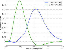
(a) Estimated components as $R$ = 2.

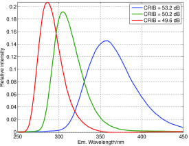
(b) Estimated components as $R$ = 3.

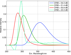
(c) Estimated components as $R$ = 4.

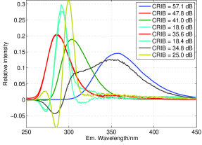
(d) Estimated components as $R$ = 8.

Figure 1: Illustration for emission components from best-fit decompositions over 100 Monte Carlo runs for example VI-A.

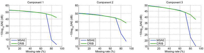
Figure 2: CRIB for the second-mode components of CP decomposition of tensor in section VI.A with missing elements and mean square angular error obtained in simulations versus percentage of the missing elements.

V-C Stability of the decomposition of Brie’s tensor

Brie et al [20] presented an example of a four-way tensor of rank 3, which arises while studying the response of bacterial bio-sensors to different environmental agents. The tensor has co-linear columns in three of four modes and the main message of the paper is that its CP decomposition is still unique. In this subsection we verify stability of the decomposition.

The factor matrices of the tensor have the form

$${\bf A}_{1}=[{\bf a}_{1},{\bf a}_{2},{\bf a}_{3}]\quad{\bf A}_{2}=[{\bf a}_{4},{\bf a}_{4},{\bf a}_{5}],\quad{\bf A}_{3}=[{\bf a}_{6},{\bf a}_{7},{\bf a}_{6}]\quad{\bf A}_{4}=[{\bf a}_{8},{\bf a}_{9},{\bf a}_{9}]~{}.$$

Assume for simplicity that all factors have unit norm, $\|{\bf a}_{n}\|=1$, $n=1,\ldots,9$. Due to Theorem 5 it holds that CRIB on ${\bf a}_{1}$ is a function of scalars $c_{11}={\bf a}_{1}^{T}{\bf a}_{2}$, $c_{12}={\bf a}_{1}^{T}{\bf a}_{3}$, $c_{13}={\bf a}_{2}^{T}{\bf a}_{3}$, $c_{2}={\bf a}_{4}^{T}{\bf a}_{5}$, $c_{3}={\bf a}_{6}^{T}{\bf a}_{7}$, $c_{4}={\bf a}_{8}^{T}{\bf a}_{9}$ and $I_{1}$, which is the dimension of ${\bf a}_{1}$. Then, the matrices ${\bf C}_{n}={\bf A}_{n}^{T}{\bf A}_{n}$, $n=2,3,4$, have the form

$${\bf C}_{2}=\left[\begin{array}[]{ccc}1&1&c_{2}\\ 1&1&c_{2}\\ c_{2}&c_{2}&1\end{array}\right],{\bf C}_{3}=\left[\begin{array}[]{ccc}1&c_{3}&1\\ c_{3}&1&c_{3}\\ 1&c_{3}&1\end{array}\right],{\bf C}_{4}=\left[\begin{array}[]{ccc}1&c_{4}&c_{4}\\ c_{4}&1&1\\ c_{4}&1&1\end{array}\right]~{}.$$

A straightforward usage of Theorem 4 is not possible, because some of the involved matrices become singular. The CRIB itself, however, is finite and can be computed using an artificial parameter $\varepsilon$ as a limit. The limit CRIB is computed for modified matrices at $\varepsilon\rightarrow 0$,

$${\bf C}_{2\varepsilon}=\left[\begin{array}[]{ccc}1&1-\varepsilon&c_{2}\\ 1-\varepsilon&1&c_{2}\\ c_{2}&c_{2}&1\end{array}\right],{\bf C}_{3\varepsilon}=\left[\begin{array}[]{ccc}1&c_{3}&1-\varepsilon\\ c_{3}&1&c_{3}\\ 1-\varepsilon&c_{3}&1\end{array}\right],{\bf C}_{4\varepsilon}=\left[\begin{array}[]{ccc}1&c_{4}&c_{4}\\ c_{4}&1&1-\varepsilon\\ c_{4}&1-\varepsilon&1\end{array}\right]~{}.$$

If any of the correlations $c_{2},c_{3},c_{4}$ is zero, it is also augmented by $\varepsilon$.

The limit CRIB can be shown to be independent of off-diagonal elements of ${\bf C}_{1}$, unless ${\bf C}_{1}$ is singular. Assume that ${\bf C}_{1}$ is regular. The result, obtained by Symbolic Matlab, is

$$\mbox{CRIB}_{\varepsilon=0}({\bf a}_{1}) = \frac{\sigma^{2}}{\|{\bf a}_{1}\|^{2}}\,\frac{1}{2c_{2}^{2}c_{3}^{2}c_{4}^{2}-c_{2}^{2}c_{3}^{2}-c_{2}^{2}c_{4}^{2}-c_{3}^{2}c_{4}^{2}+1}\Biggl{[}(I_{1}-1)(1-c_{2}^{2}c_{3}^{2})$$ (64)

$$-\frac{c_{3}^{4}(c_{2}^{2}+1)-3c_{3}^{2}+1}{1-c_{3}^{2}}-\frac{c_{2}^{4}(c_{3}^{2}+1)-3c_{2}^{2}+1}{1-c_{2}^{2}}+\frac{2-c_{2}^{2}-c_{3}^{2}}{1-c_{4}^{2}}\Biggr{]}~{}.$$

It follows that the decomposition is stable, unless all three factors in some mode are collinear.

V-D Maximum Stable Rank

A theoretically interesting question is, what is the maximum rank of a tensor of a given dimension which has a stable CP decomposition (with finite CRIB). For easy reference, we shall call it maximum stable rank and denote it $R_{smax}(I_{1},\ldots,I_{N})$.

An upper bound for the maximum stable rank can be deduced from the requirement that the number of free parameters in the model, which is $R(\sum_{n=1}^{N}I_{n}-N+1)$ in CP decomposition, cannot exceed dimension of the available data, which is $\prod_{n=1}^{N}I_{n}$. It follows that

$$R_{smax}(I_{1},\ldots,I_{N})\leq\left\lfloor\frac{\prod_{n=1}^{N}I_{n}}{\sum_{n=1}^{N}I_{n}-N+1}\right\rfloor$$ (65)

where $\lfloor x\rfloor$ denotes the lower integer part of $x$. It can be verified numerically that for many (and maybe all) tensor dimensions, an equality in (65) holds. In other words, it means that the CRIB computed, e.g., via Theorem 4 for a CP decomposition with rank $R=R_{smax}$ and some (e.g. random) factor matrices is finite. For example, the maximum stable rank is $R_{smax}=2$ for $2\times 2\times 2$ tensors, and $R_{smax}=3$ for $3\times 3\times 3$ tensors. For order-8 tensors of dimension $2\times\ldots\times 2$, $(8\times)$, it holds $R_{smax}=28$.

It might be interesting to compare the maximum stable rank with the maximum rank and the maximum typical rank (to be explained below) for given tensor dimension, if they are known [44]. If the elements of a tensor are chosen randomly according to a continuous probability distribution, there is not a rank which occurs with probability 1 in general. Such rank, if exists, is called generic. Ranks which occur with strictly positive probabilities are called typical ranks. For example it was computed in [10] that probability for a real random Gaussian tensor of the size $2\times 2\times 2$ to be 2 and 3 is $\pi/4$, and $1-\pi/4$, respectively. We can see that no tensor of the rank 3 and the dimension has a stable decomposition. For tensors of the dimension $3\times 3\times 3$ the typical rank is 5 [10], it is a generic rank - but no decomposition of these rank-5 tensors is stable, as $R_{smax}=3$.

Next, it might be interesting to compare the maximum stable rank with the maximum rank for unique tensor decomposition, or prove that these two coincide. Liu and Sidiropoulos [11, 29] derived a necessary condition for uniqueness of the CP decomposition, which, according to a formulation in [43] reads

$$\min_{n=1,\ldots,N}\mbox{rank}\left({\bf A}_{1}\odot\ldots\odot{\bf A}_{n-1}\odot{\bf A}_{n+1}\odot\ldots\odot{\bf A}_{N}\right)=R$$ (66)

where $\odot$ means the Khatri-Rao product. The condition (66) is equivalent to the condition that the matrices $\mbox{\boldmath{$\Xi$}}_{n}={\bf A}_{1}\odot\ldots\odot{\bf A}_{n-1}\odot{\bf A}_{n+1}\odot\ldots\odot{\bf A}_{N}$ have all full column rank, $n=1,\ldots,N$, which is further equivalent to the condition that the product $\mbox{\boldmath{$\Xi$}}_{n}^{T}\mbox{\boldmath{$\Xi$}}_{n}$ are regular for $n=1,\ldots,N$. Finally note that

$$\mbox{\boldmath{$\Xi$}}_{n}^{T}\mbox{\boldmath{$\Xi$}}_{n}=\mbox{\boldmath$\Gamma$}_{nn},\qquad n=1,\ldots,N~{}.$$

where $\mbox{\boldmath$\Gamma$}_{nn}$ was defined in (5) and appears in computation of the CRIB.

Unfortunately, it appears that the condition (66) is only necessary, but not sufficient for uniqueness. It is often fulfilled for $R$ higher than $R_{smax}$. Thus a relation between the stability and uniqueness of the CP decomposition remains open question for now.

VI Conclusions

Cramér-Rao bounds for CP tensor decomposition represent an important tool for studying accuracy and stability of the decomposition. The bounds derived in this manuscript serve as a theoretical support for a method of the decomposition through tensor reshaping [32]. As a side result, a novel method of inverting Hessian matrix, which is more computationally efficient, is derived for the problem. It enables a further improvement of speed of the fast Gauss-Newton for the problem [26]. A novel expression for Hessian for CP decomposition of tensor with missing entries has been derived. It can serve for assessing accuracy of CP decomposition of these tensors without need of long Monte Carlo simulations, and for implementing a damped Gauss-Newton algorithm for CP decomposition of these tensors.

A direct link between stability and essential uniqueness remains to be an open theoretical question. In particular, it is not known yet for sure if stability implies the essential uniqueness.

CRB expressions similar to the ones derived in this paper can be also derived for other important special tensor decomposition models such as INDSCAL (where two or more factor matrices coincide) [16, 37], or for the PARALIND model, where the factor matrices have certain structure [22], and for block factorization methods.

Appendix A

Matrix Inversion Lemma (Woodbury identity)
Let ${\bf A}$, ${\bf X}$, ${\bf Y}$, and ${\bf R}$ are matrices of compatible dimensions such that the following products and inverses exist. Then

$$({\bf A}+{\bf X}{\bf R}{\bf Y})^{-1}={\bf A}^{-1}-{\bf A}^{-1}{\bf X}({\bf R}^{-1}+{\bf Y}{\bf A}^{-1}{\bf X})^{-1}{\bf Y}{\bf A}^{-1}~{}.$$ (67)

Appendix B

Proof of Theorem 4
Let the matrices ${\bf K}$ and $\Psi$ in (18) be partitioned as

$${\bf K}=\left[\begin{array}[]{cc}{\bf 0}&{\bf K}_{1}\\ {\bf K}_{1}^{T}&{\bf K}_{2}\end{array}\right],\qquad\mbox{\boldmath{$\Psi$}}=\left[\begin{array}[]{cc}\mbox{\boldmath{$\Psi$}}_{1}&{\bf 0}\\ {\bf 0}&\mbox{\boldmath{$\Psi$}}_{2}\end{array}\right]$$ (72)

where the left-upper blocks have the size $R^{2}\times R^{2}$. Then, using a formula for inverse of partitioned matrices, the left-upper block of ${\bf B}$ in (18) can be written as

$${\bf B}_{0}={\bf K}_{1}({\bf I}_{(N-1)R^{2}}+\mbox{\boldmath{$\Psi$}}_{2}{\bf K}_{2}-\mbox{\boldmath{$\Psi$}}_{2}{\bf K}_{1}^{T}\mbox{\boldmath{$\Psi$}}_{1}{\bf K}_{1})^{-1}\mbox{\boldmath{$\Psi$}}_{2}{\bf K}_{1}^{T}\stackrel{{\scriptstyle\triangle}}{{=}}{\bf K}_{1}{\bf K}_{3}^{-1}\mbox{\boldmath{$\Psi$}}_{2}{\bf K}_{1}^{T}~{}.$$ (73)

A key observation which enables a fast inversion of the term ${\bf K}_{3}$ is that

$${\bf K} = {\bf K}_{0}+{\bf D}{\bf F}{\bf D}^{T}$$ (74)

where

$${\bf K}_{0} = -{\tt{bdiag}}\left({\bf P}_{R}{\bf F}({\tt dvec}(1\oslash{\bf C}_{n}))^{2}\right)_{n=1}^{N}$$ (75)

$${\bf F} = {\bf P}_{R}\,\prod_{n=1}^{N}{\tt dvec}({\bf C}_{n})={\bf P}_{R}\,{\tt dvec}(\mbox{\boldmath$\Gamma$}_{11}\circledast{\bf C}_{1})$$ (76)

$${\bf D} = \left[{\tt dvec}(1\oslash{\bf C}_{1}),\ldots,{\tt dvec}(1\oslash{\bf C}_{N})\right]^{T}~{}.$$ (77)

Similarly,

$${\bf K}_{2} = {\bf K}_{02}+{\bf D}_{2}{\bf F}{\bf D}_{2}^{T}$$ (78)

where

$${\bf K}_{02} = -{\tt{bdiag}}\left({\bf P}_{R}{\bf F}({\tt dvec}(1\oslash{\bf C}_{n}))^{2}\right)_{n=2}^{N}$$ (79)

$${\bf D}_{2} = \left[{\tt dvec}(1\oslash{\bf C}_{2}),\ldots,{\tt dvec}(1\oslash{\bf C}_{N})\right]^{T}~{}.$$ (80)

Then the matrix ${\bf K}_{3}$ in (73) can be written as

$${\bf K}_{3} = {\bf I}_{(N-1)R^{2}}+\mbox{\boldmath{$\Psi$}}_{2}{\bf K}_{2}-\mbox{\boldmath{$\Psi$}}_{2}{\bf K}_{1}^{T}\mbox{\boldmath{$\Psi$}}_{1}{\bf K}_{1}$$ (81)

$$= {\bf I}_{(N-1)R^{2}}+\mbox{\boldmath{$\Psi$}}_{2}({\bf K}_{02}-{\bf K}_{1}^{T}\mbox{\boldmath{$\Psi$}}_{1}{\bf K}_{1})+\mbox{\boldmath{$\Psi$}}_{2}{\bf D}_{2}{\bf F}{\bf D}_{2}^{T}$$

$$= {\bf Q}+\mbox{\boldmath{$\Psi$}}_{2}{\bf D}_{2}{\bf F}{\bf D}_{2}^{T}$$

where

$${\bf Q} = {\tt{bdiag}}({\bf Q}_{n})_{n=2}^{N}$$ (82)

$${\bf Q}_{n} = {\bf I}_{R^{2}}-(\mbox{\boldmath$\Gamma$}_{nn}^{-1}\otimes{\bf X}_{n}){\bf P}_{R}\,({\bf F}({\tt dvec}(1\oslash{\bf C}_{n}))^{2}+{\tt dvec}(\mbox{\boldmath$\Gamma$}_{1n})(\mbox{\boldmath$\Gamma$}_{11}^{-1}\otimes{\bf C}_{1}){\tt dvec}(\mbox{\boldmath$\Gamma$}_{1n}){\bf P}_{R})~{}.$$ (83)

Now, ${\bf K}_{3}$ can be easily inverted using the matrix inversion lemma (67),

$${\bf K}_{3}^{-1} = {\bf Q}^{-1}-{\bf Q}^{-1}{\bf D}_{2}^{T}({\bf I}_{R^{2}}+{\bf D}_{2}^{T}{\bf Q}^{-1}\mbox{\boldmath{$\Psi$}}_{2}{\bf D}_{2}{\bf F})^{-1}\mbox{\boldmath{$\Psi$}}_{2}{\bf D}_{2}{\bf F}{\bf Q}^{-1}~{}.$$ (84)

Inserting (84) in (73) gives, after some simplifications, the result (35).  

Appendix C

Proof of Theorem 5
Consider the change of scale of columns of factor matrices up to their first columns. As in Section II assume that the scale change is realized in ${\bf A}_{1}$, while the other factor matrices have columns of unit norm. The theorem claims that the substitution ${\bf A}_{1}\leftarrow{\bf A}_{1}{\bf D}$ into (27) where ${\bf D}={\tt{diag}}(1,\lambda_{2},\dots,\lambda_{R})$, $\lambda_{r}\neq 0$, has no influence on $\mbox{CRIB}({\bf a}_{1})$.

The substitution ${\bf A}_{1}\leftarrow{\bf A}_{1}{\bf D}$ leads to ${\bf C}_{1}\leftarrow{\bf D}{\bf C}_{1}{\bf D}$ and ${\bf X}_{1}\leftarrow{\bf D}{\bf X}_{1}{\bf D}$ while ${\bf C}_{n}$ and ${\bf X}_{n}$, $n=2,\dots,N$, remain the same. Consequently, $\mbox{\boldmath$\Gamma$}_{1n}$, $n=1,\dots,N$, remain unchanged while $\mbox{\boldmath$\Gamma$}_{nn}\leftarrow{\bf D}\mbox{\boldmath$\Gamma$}_{nn}{\bf D}$ for $n=2,\dots,N$. Now, we can substitute into (35) assuming that the condition of Theorem 4 is satisfied.

Let $\widetilde{{\bf S}}_{n}$ denote the matrix ${\bf S}_{n}$ in (39) after the substitution ${\bf A}_{1}\leftarrow{\bf A}_{1}{\bf D}$. It can be shown that $({\bf D}\otimes{\bf I}_{R})\widetilde{{\bf S}}_{n}={\bf S}_{n}({\bf D}\otimes{\bf I}_{R})$ using the rules

$$({\bf D}\mbox{\boldmath$\Gamma$}_{nn}{\bf D})^{-1}\otimes{\bf X}_{n} =({\bf D}^{-1}\otimes{\bf I}_{R})(\mbox{\boldmath$\Gamma$}_{nn}^{-1}\otimes{\bf X}_{n})({\bf D}^{-1}\otimes{\bf I}_{R})$$ (85)

$${\tt dvec}({\bf D}\mbox{\boldmath$\Gamma$}_{nn}{\bf D}\oslash{\bf C}_{n}) =({\bf D}\otimes{\bf D}){\tt dvec}(\mbox{\boldmath$\Gamma$}_{nn}\oslash{\bf C}_{n})$$ (86)

$$({\bf I}_{R}\otimes{\bf D}){\bf P}_{R} ={\bf P}_{R}({\bf D}\otimes{\bf I}_{R})$$ (87)

and the fact that diagonal matrices commute. Using the same rules in further substitutions, after some computations, the independence of $\mbox{CRIB}({\bf a}_{1})$ on ${\bf D}$ follows.

Appendix D

Proof of Theorem 6
Again, assume for simplicity that all factors have unit norms. It holds

$$\mbox{\boldmath$\Gamma$}_{11}=\left[\begin{array}[]{cc}1&h_{1}\\ h_{1}&1\end{array}\right],\quad{\bf X}_{n}=\left[\begin{array}[]{cc}0&0\\ 0&1-c_{n}^{2}\end{array}\right],\quad n=1,\ldots,N~{}.$$

and

$$g_{11} = [\mbox{\boldmath$\Gamma$}_{11}^{-1}]_{11}=\frac{1}{1-h_{1}^{2}}$$ (88)

$${\bf g}_{1,:} = g_{11}\left[1,\quad-h_{1}\right]~{}.$$ (89)

The matrix $\Psi$ in (32) can be decomposed as $\mbox{\boldmath{$\Psi$}}={\bf J}\mbox{\boldmath{$\Phi$}}$ where

$${\bf J} = {\tt{bdiag}}\left({\bf I}_{4},{\bf I}_{2}\otimes[0,\,1]^{T},\ldots,{\bf I}_{2}\otimes[0,\,1]^{T}\right)$$ (90)

$$\Phi = {\tt{bdiag}}\left(\mbox{\boldmath$\Gamma$}_{11}^{-1}\otimes{\bf C}_{1},(1-c_{2}^{2})\mbox{\boldmath$\Gamma$}_{22}^{-1}\otimes[0,\,1],\ldots,(1-c_{N}^{2})\mbox{\boldmath$\Gamma$}_{NN}^{-1}\otimes[0,\,1]\right)~{}.$$ (91)

Then the matrix ${\bf B}$ in (18) can be rewritten using the Woodbury identity (67) as

$${\bf B} = {\bf K}({\bf I}_{4N}+{\bf J}\mbox{\boldmath{$\Phi$}}{\bf K})^{-1}={\bf K}-{\bf K}{\bf J}({\bf I}_{2N+2}+\mbox{\boldmath{$\Phi$}}{\bf K}{\bf J})^{-1}\mbox{\boldmath{$\Phi$}}{\bf K}~{}.$$ (92)

Now, put ${\bf B}_{4}={\bf I}_{2N+2}+\mbox{\boldmath{$\Phi$}}{\bf K}{\bf J}$ and write it in the block form as

$${\bf B}_{4} = {\bf I}_{2N+2}+\mbox{\boldmath{$\Phi$}}{\bf K}{\bf J}=\left[\begin{array}[]{cc}{\bf B}_{41}&{\bf B}_{42}\\ {\bf B}_{43}&{\bf B}_{44}\end{array}\right]$$ (95)

where ${\bf B}_{41}$ has the size $4\times 4$. The bottom-right block ${\bf B}_{44}$ of dimension $(2N-2)\times(2N-2)$ is easy to be inverted using the Woodbury identity again, because it can be written as

$${\bf B}_{44} = {\bf B}_{5}+{\bf s}{\bf f}^{T}$$ (96)

where

$${\bf B}_{5} = {\tt{bdiag}}\left({\bf B}_{52},\ldots,{\bf B}_{5N}\right)$$ (97)

$${\bf B}_{5n} = \left[\begin{array}[]{cc}1&-\frac{h_{n}c_{1}(1-c_{n}^{2})}{1-h_{n}^{2}c_{1}^{2}}\\ 0&\frac{c_{n}^{2}-h_{n}^{2}c_{1}^{2}}{1-h_{n}^{2}c_{1}^{2}}\end{array}\right],\qquad n=2,\ldots,N$$ (100)

$${\bf s} = \left[-\frac{h_{2}c_{1}(1-c_{2}^{2})}{1-h_{2}^{2}c_{1}^{2}},\frac{(1-c_{2}^{2})}{1-h_{2}^{2}c_{1}^{2}},\ldots,-\frac{h_{N}c_{1}(1-c_{N}^{2})}{1-h_{N}^{2}c_{1}^{2}},\frac{(1-c_{N}^{2})}{1-h_{N}^{2}c_{1}^{2}}\right]^{T}$$ (101)

$${\bf f} = [0,\,1,\,0,\,1,\ldots,1]^{T}~{}.$$ (102)

After some computations, we receive the result (44).  

Appendix E

Proof of Theorem 7

Under the assumption of the Theorem, it holds that the matrix ${\bf C}_{1}={\bf A}_{1}^{T}{\bf A}_{1}$ is diagonal and ${\bf C}_{2}={\bf I}_{R}$ (identity matrix). Thanks to Theorem 5 we can assume, without any loss of generality, that ${\bf C}_{1}={\bf I}_{R}$ as well. It can be shown for $\mbox{\boldmath$\Gamma$}_{mn}$ in (5) that $\mbox{\boldmath$\Gamma$}_{mn}={\bf I}_{R}$ for all pairs $(m,n)$, $(m,n)\neq(1,2),(2,1)$. Only $\mbox{\boldmath$\Gamma$}_{12}$ and $\mbox{\boldmath$\Gamma$}_{21}=\mbox{\boldmath$\Gamma$}_{12}$ are possibly different. Note that the first row of $\mbox{\boldmath$\Gamma$}_{12}$ is $(1,\gamma_{2},\ldots,\gamma_{N})$.

It follows from these observations that all non-diagonal $R^{2}\times R^{2}$ blocks ${\bf K}_{mn}$ of ${\bf K}$ in (6) with $(m,n)\neq(1,2),(2,1)$ are identical, diagonal, having 1 at positions $(p,p)$, $p=1,R+1,2R+2,\ldots,R^{2}$ and 0 elsewhere. In other words, these ${\bf K}_{mn}$ can be written as ${\bf K}_{mn}={\bf Q}{\bf Q}^{T}$, where ${\bf Q}$ is a 0-1 matrix of the size $R^{2}\times R$, the $p-$th column of ${\bf Q}$ has the value 1 at position $(p-1)(R+1)+1$ and 0 elsewhere.

Computation of the CRIB can proceed from equation (73) by inserting the special form of the blocks of ${\bf K}_{1}$ and ${\bf K}_{2}$ and using the Woodbury identity (67).  

Appendix F

Proof of Theorem 8

The following identities are used in this proof

$$\operatorname{vec}\left({\bf A}\circledast{\bf B}\right) = \operatorname{dvec}({\bf B})\,\operatorname{vec}\left({\bf A}\right),$$ (103)

$${\bf a}^{T}\,\operatorname{diag}({\bf b})\,{\bf c} = \left({\bf a}\circledast{\bf c}\right)^{T}{\bf b},$$ (104)

$$({\bf a}\otimes{\bf b})\circledast({\bf c}\otimes{\bf d}) = ({\bf a}\circledast{\bf c})\otimes({\bf b}\circledast{\bf d})~{}.$$ (105)

Here, dimensions of ${\bf a}$, ${\bf b}$, ${\bf c}$ and ${\bf d}$ are assumed to match accordingly.

The approximate Hessian in (59) is given by

$${\bf H}={\bf J}_{W}^{T}(\mbox{\boldmath{$\theta$}}){\bf J}_{W}(\mbox{\boldmath{$\theta$}})={\bf J}(\mbox{\boldmath{$\theta$}})^{T}\operatorname{dvec}(\boldsymbol{\mathscr{{W}}}){\bf J}(\mbox{\boldmath{$\theta$}}),$$ (106)

where ${\bf J}(\mbox{\boldmath{$\theta$}})$ is the Jacobian for the complete data.

We have

$$\frac{\partial\operatorname{vec}\left(\boldsymbol{\mathscr{{Y}}}\right)}{\partial{\bf a}^{(n)}_{ir}} = \left(\bigotimes_{k=n+1}^{N}{\bf a}^{(k)}_{r}\right)\otimes{\bf e}^{(n)}_{i}\otimes\left(\bigotimes_{k=1}^{n-1}{\bf a}^{(k)}_{r}\right)\,,$$ (107)

where unit vector ${\bf e}^{(n)}_{i}$ for $i=1,2,\ldots,I_{n}$ is the $i$-th column of the identity matrix of size ${I_{n}\times I_{n}}$.

An $(i,j)$ entry of a sub matrix ${\bf H}^{(n,n)}_{r,s}$ for $i=1,2,\ldots,I_{n}$, and $j=1,2,\ldots,I_{n}$ is given by

$${\bf H}^{(n,n)}_{r,s}(i,j) = \left(\frac{\partial\operatorname{vec}\left(\boldsymbol{\mathscr{{Y}}}\right)}{\partial{\bf a}^{(n)}_{ir}}\right)^{T}\,\operatorname{dvec}{\left(\boldsymbol{\mathscr{{W}}}\right)}\;\left(\frac{\partial\operatorname{vec}\left(\boldsymbol{\mathscr{{Y}}}\right)}{\partial{\bf a}^{(n)}_{js}}\right)$$ (108)

$$= \left(\left(\bigotimes_{k=n+1}^{N}{\bf a}^{(k)}_{r}\circledast{\bf a}^{(k)}_{s}\right)\otimes\left({\bf e}^{(n)}_{i}\circledast{\bf e}^{(n)}_{j}\right)\otimes\left(\bigotimes_{k=1}^{n-1}{\bf a}^{(k)}_{r}\circledast{\bf a}^{(k)}_{s}\right)\right)^{T}\;\operatorname{vec}\left(\boldsymbol{\mathscr{{W}}}\right)$$

$$= \boldsymbol{\mathscr{{W}}}\;{\bar{\times}}_{-n}\{{\bf b}^{(k)}\}\;{\bar{\times}}_{n}\,\delta_{ij}\,{\bf e}^{(n)}_{i}\,,$$

where $\delta_{ij}$ is the Kronecker delta, ${\bf b}^{(n)}={\bf a}^{(n)}_{r}\circledast{\bf a}^{(n)}_{s}$, for $n=1,\ldots,N$. This leads to that a diagonal sub-matrix ${\bf H}^{(n,n)}_{r,s}$ is a diagonal matrix as in Theorem IV.

For off-diagonal sub matrices ${\bf H}^{(n,m)}_{r,s}$ of size $I_{n}\times I_{m}$ ($1\leq n<m\leq N$), we have

$${\bf H}^{(n,m)}_{r,s}(i,j) = \left(\frac{\partial\operatorname{vec}\left(\boldsymbol{\mathscr{{Y}}}\right)}{\partial{\bf a}^{(n)}_{ir}}\right)^{T}\,\operatorname{dvec}{\left(\boldsymbol{\mathscr{{W}}}\right)}\;\left(\frac{\partial\operatorname{vec}\left(\boldsymbol{\mathscr{{Y}}}\right)}{\partial{\bf a}^{(m)}_{js}}\right)$$ (109)

$$= \left(\left(\bigotimes_{k=m+1}^{N}{\bf a}^{(k)}_{r}\circledast{\bf a}^{(k)}_{s}\right)\otimes\left({\bf a}^{(m)}_{r}\circledast{\bf e}^{(m)}_{j}\right)\otimes\left(\bigotimes_{k=n+1}^{m-1}{\bf a}^{(k)}_{r}\circledast{\bf a}^{(k)}_{s}\right)\otimes\right.$$

$$\left.\left({\bf e}^{(n)}_{i}\circledast{\bf a}^{(n)}_{s}\right)\otimes\left(\bigotimes_{k=1}^{n-1}{\bf a}^{(k)}_{r}\circledast{\bf a}^{(k)}_{s}\right)\right)^{T}\;\operatorname{vec}\left(\boldsymbol{\mathscr{{W}}}\right)$$

$$= a^{(m)}_{jr}\,a^{(n)}_{is}\,\left(\boldsymbol{\mathscr{{W}}}{\bar{\times}}_{-\{n,m\}}\,\{{\bf b}^{(k)}\}\;{\bar{\times}}_{n}{\bf e}^{(n)}_{i}\;{\bar{\times}}_{m}{\bf e}^{(m)}_{j}\ \right).$$

This leads to the compact form in Theorem 8.

References

- [1] R. Bro, Multi-way Analysis in the Food Industry Models, Algorithms, and Applications, University of Amsterdam, http://www/models.life.ku.dk/research/theses/, 1998.
- [2] P.M. Kroonenberg, Applied Multiway Data Analysis, Wiley, 2008.
- [3] A. Smilde, R. Bro, P. Geladi, Multi-way Analysis: Applications in the Chemical Sciences, Wiley, 2004.
- [4] A. Cichocki, R. Zdunek, A. H. Phan and S. I. Amari, Nonnegative Matrix and Tensor Factorizations: Applications to Exploratory Multi-way Data Analysis and Blind Source Separation, Wiley, 2009.
- [5] V. De Silva, L.-H. Lim, “Tensor rank and the ill-posedness of the best low-rank approximation problem,” SIAM Journal on Matrix Analysis and Applications, vol. 30, pp. 1084–1127, 2008.
- [6] W.P. Krijnen, T.K. Dijkstra, and A. Stegeman, “On the non-existence of optimal solutions and the occurrence of “degeneracy” in the Candecomp/Parafac model, Psychometrika, vol. 73, pp. 431–439, 2008.
- [7] R.A. Harshman, “Foundations of the PARAFAC procedure: model and conditions for an “explanatory” multimode factor analysis”, UCLA Working Papers Phonet. vol. 16, pp. 1-84, 1970.
- [8] R.A. Harshman, “Determination and proof of minimum uniqueness conditions for PARAFAC”, UCLA Working Papers Phonet. vol. 22, pp. 111-117, 1972.
- [9] J. B. Kruskal, “Three-way arrays: Rank and uniqueness of trilinear decompositions, with application to arithmetic complexity and statistics, ” Linear Algebra Appl., vol. 18, pp. 95-138, 1977.
- [10] J B Kruskal, “Rank, decomposition, and uniqueness for 3-way and N-way arrays” in Multiway data analysis, pp. 7 18, North-Holland (Amsterdam), 1989.
- [11] N. D. Sidiropoulos and R. Bro, “On the uniqueness of multilinear decomposition of N-way arrays,” J. Chemometrics, vol. 14, pp. 229 239, May 2000.
- [12] J. M. F. Ten Berge, and N.D. Sidiropoulos, “On Uniqueness in CANDECOMP / PARAFAC,” Psychometrika, Vol. 67, No. 3, pp.399–409, Sep. 2002.
- [13] T. Jiang, N.D. Sidiropoulos, “Kruskal’s permutation lemma and the identification of Candecomp/Parafac and bilinear models with constant modulus constraints. IEEE Transactions on Signal Processing, vol. 52, pp. 2625–2636. (2004)
- [14] L. De Lathauwer, “A link between the canonical decomposition in multilinear algebra and simultaneous matrix diagonalization”, SIAM Journal on Matrix Analysis and Applications, vol. 28, pp. 642–666, 2006.
- [15] A. Stegeman, N.D. Sidiropoulos, “On Kruskal’s uniqueness condition for the Candecomp/Parafac decomposition”, Linear Algebra and its Applications, vol. 420, pp. 540–552, 2007.
- [16] A. Stegeman, “On uniqueness conditions for Candecomp/Parafac and Indscal with full column rank in one mode,” Linear Algebra and its Applications, Vol. 431, No. 1–2, pp. 211–227, 2009.
- [17] A. Stegeman and A.L.F. de Almeida, “Uniqueness conditions for constrained three-way factor decompositions with linearly dependent loadings,” SIAM Journal on Matrix Analysis and Applications, Vol. 31, No. 3, pp. 1469–1490, Aug. 2009.
- [18] A. Stegeman, “On uniqueness of the n-th order tensor decomposition into rank-1 terms with linear independence in one mode,” SIAM Journal on Matrix Analysis and Applications, Vol. 31, No. 5, pp. 2498–2516, 2010.
- [19] A. Stegeman, “On uniqueness of the canonical tensor decomposition with some form of symmetry,” SIAM Journal on Matrix Analysis and Applications, Vol. 32, No. 3, pp. 561–583, 2011.
- [20] D. Brie, S. Miron, F. Caland and C. Mustin, “An uniqueness condition for the 4-way CANDECOMP/PARAFAC model with collinear loadings in three modes”, Proc. ICASSP 2011, pp. 4112–4115, 2011.
- [21] I. Domanov and L. De Lathauwer, “On the Uniqueness of the Canonical Polyadic Decomposition Part II: Overall Uniqueness, ESAT, KU Leuven, ESAT-SISTA Internal Reports 12-90, 2012.
- [22] X. Guo, S. Miron, D. Brie, and A. Stegeman, “Uni-mode and Partial Uniqueness Conditions for CANDECOMP/PARAFAC of Three-Way Arrays with Linearly Dependent Loadings, ” SIAM Journal on Matrix Analysis and Applications, Vol. 33, No. 1, pp. 111–129, 2012.
- [23] S. Basu and Y. Bresler, ”The stability of nonlinear least squares problems and the Cramér-Rao bound,” IEEE Trans. Signal Processing, vol. 48, pp. 3426-3436, Dec. 2000.
- [24] G. Tomasi and R. Bro, “A comparison of algorithms for fitting the PARAFAC model, Computational Statistics and Data Analysis, vol. 50, no.7, pp. 1700–1734, April 2006.
- [25] P. Paatero, “A weighted non-negative least squares algorithm for three-way ’PARAFAC’ factor analysis”, Chemometrics and Intelligent Laboratory Systems, vol. 38, pp. 223–242, 1997.
- [26] A.-H. Phan, P. Tichavský, and A. Cichocki, “Low Complexity Damped Gauss-Newton Algorithms for CANDECOMP/PARAFAC”, SIAM, SIMAX (accepted for publication), available at http://arxiv.org/abs/1205.2584.
- [27] P. Tichavský and Z. Koldovský, “Stability of CANDECOMP-PARAFAC tensor decomposition”, Proc. ICASSP 2011, Prague, Czech Republic, pp. 4164-4167, 2011.
- [28] P. Tichavský and Z. Koldovský, ”Weight Adjusted Tensor Method for Blind Separation of Underdetermined Mixtures of Nonstationary Sources, ” IEEE Trans. on Signal Processing, Vol. 59, No. 3, pp. 1037–1047, March 2011.
- [29] X. Liu, and N.D. Sidiropoulos, “Cramér-Rao Lower Bounds for Low-rank Decomposition of Multidimensional Arrays,” IEEE Trans. on Signal Processing, vol. 49, no. 9, pp. 2074–2086, Sep. 2001.
- [30] T. Jiang, and N.D. Sidiropoulos, ”Blind Identification of Out of Cell Users in DS-CDMA”, EURASIP Journal on Applied Signal Processing (JASP), special issue on Advances in Smart Antennas, 2004(9):1212-1224, Aug. 2004.
- [31] Z. Koldovský, P. Tichavský, and Anh Huy Phan, ”Stability Analysis and Fast Damped-Gauss-Newton Algorithm for INDSCAL Tensor Decomposition,” Proc. of IEEE Workshop on Statistical Signal Processing, pp. 581–584, Nice, France, June 2011.
- [32] A.-H. Phan, P. Tichavský, and A. Cichocki, “CANDECOMP/PARAFAC Decomposition of High-order Tensors Through Tensor Reshaping”, submitted.
- [33] R. Bro, R. A. Harshman, N. D. Sidiropoulos, and M. E. Lundy, “Modeling multi-way data with linearly dependent loadings,” Journal of Chemometrics, vol. 23, no. 7-8, pp. 324 340, 2009.
- [34] M. B. Dosse, J. M.F. Berge, and J. N. Tendeiro, “Some new results on orthogonally constrained candecomp,” Journal of Classification, vol. 28, pp. 144 155, 2011.
- [35] M. Sorensen, L. De Lathauwer, P. Comon, S. Icart, and L. Deneire, “Canonical polyadic decomposition with orthogonality constraints,” SIAM Journal on Matrix Analysis and Applications, p. accepted, 2012.
- [36] J. Chen and Y. Saad, “On the Tensor SVD and the Optimal Low Rank Orthogonal Approximation of Tensors”, Vol. 30, pp. 1709–1734, 2009.
- [37] J. Tendeiro, M. Bennani Dosse, and J.M.F. Ten Berge, “First and second-order derivatives for CP and INDSCAL”. Chemometrics and Intelligent Laboratory Systems, vol. 106, pp.27–36, 2011.
- [38] A. Householder, The Theory of Matrices in Numerical Analysis. New York: Blaisdell Publishing Co., 1964.
- [39] G. Tomasi and R. Bro, “PARAFAC and missing values”, Chemometrics and Intelligent Laboratory Systems, vol. 75, pp. 163–180, 2005.
- [40] R. Bro (1999), Exploratory study of sugar production using fluorescence spectroscopy and multi-way analysis. Chemom. Intell. Lab. Syst, 46, 133–147.
- [41] R. Bro (1998), Multi-way Analysis in the Food Industry - Models, Algorithms, and Applications, PhD thesis, University of Amsterdam, Holland.
- [42] B. Porat, Digital Processing of Random Signals, Prentice Hall, 1994.
- [43] T.G. Kolda and B.W. Bader, “Tensor decompositions and applications, SIAM Review, vol. 51, no. 3, pp. 455–500, September 2009.
- [44] P. Comon, J.M.F. ten Berge, L. De Lathauwer and J. Castaing, “Generic and Typical Ranks of Multi-Way Arrays”, Linear Algebra and its Applications, vol. 430, no. 11 (2009), pp. 2997-3007, 2009.
- [45] T.G. Kolda, “Orthogonal tensor decompositions”, SIAM Journal of Matrix Analysis and Applications, vol. 23, pp. 243–255, 2001.
- [46] “A further improvement of a fast damped Gauss–Newton algorithm for CP tensor decomposition”, submitted to icassp 2013.