Averaging Complex Subspaces via a Karcher Mean Approach

Abstract

We propose a conjugate gradient type optimization technique for the computation of the Karcher mean on the set of complex linear subspaces of fixed dimension, modeled by the so-called Grassmannian. The identification of the Grassmannian with Hermitian projection matrices allows an accessible introduction of the geometric concepts required for an intrinsic conjugate gradient method. In particular, proper definitions of geodesics, parallel transport, and the Riemannian gradient of the Karcher mean function are presented. We provide an efficient step-size selection for the special case of one dimensional complex subspaces and illustrate how the method can be employed for blind identification via numerical experiments.

1 Introduction

In a wide range of signal processing applications and methods, subspaces of a fixed dimension play an important role. Signal and noise subspaces of covariance matrices are well studied objects in classical applications, such as subspace tracking [1] or direction of arrival estimation [2]. More recently, a significant amount of work is focussed on applying subspace based methods to image and video analysis [3], as well as to matrix completion problems [4]. One fundamental challenge amongst these works is the study of the statistical properties of distributions of subspaces. Specifically, in the present work, we are interested in computing the mean of a set of subspaces of equal dimension via averaging.

The averaging process, considered in this paper, employs the intrinsic geometric structure of the underlying set and is also known as the computation of the Karcher mean (in differential geometry, [5]), Fréchet mean or barycentre (statistics), geometric mean (linear algebra and matrix analysis), or center of mass (physics). General concepts of a geometric mean have been extensively studied from both theoretical and practical points of view. To mention just a few, they include probability theory and shape spaces [6, 7], imaging [8], linear algebra and matrix analysis [9], interpolation [10], and convex and differential geometry [11, 12].

An appropriate mathematical framework is given by the so-called Grassmannian, which assigns a differentiable manifold structure to the set of subspaces of equal dimension. Usually, this is achieved by identification with a matrix quotient space. In this work, we do not follow such an approach. By following [14] instead, we identify the set of subspaces of equal dimension with a set of matrices. More precisely, we consider the set of Hermitian projectors of fixed rank, which inherits its differentiable structure from the surrounding vector space of Hermitian matrices. In contrast to [14], we consider the complex case here. The identification of the complex Grassmannian with Hermitian projection matrices allows an accessible introduction of the geometric concepts such as geodesics, parallel transport, and the Riemannian gradient of the Karcher mean function.

In general, computing the Karcher mean on a smooth manifold involves a process of optimization, which by its own is of both theoretical and practical interest. Various numerical methods have been developed on the Grassmannian, such as a direct method [15], gradient descent algorithms [16], Newton’s method [14], and conjugate gradient methods [17, 18].

In this work, we focus on the development of conjugate gradient methods. These methods have been proven to be efficient in many applications due to their trade-off between computational complexity and excellent convergence properties. In particular, we propose an efficient step-size selection for the interesting case where the Grassmannian is equal to the complex projective space. Moreover, we outline how the developed method can be employed for blind identification.

The paper is organized as follows. Section 2 recalls some basic concepts in differential geometry, which make the present work intuitive and self-contained. An abstract framework of conjugate gradient methods on smooth manifolds is given in Section 3. In Section 4, the geometry of the Grassmannian is presented, followed by a detailed analysis of the of the Karcher mean function in Section 5. A geometric CG algorithm is given in Section 6 for the computation of the Karcher mean on the Grassmannian in general, together with a particularly efficient step-size selection for the special case of the complex projective space. In Section 7, we outline how the proposed approach of averaging subspaces is evidenced to be useful in blind identification and a conclusion is drawn in Section 8.

2 Differential geometric concepts

In this section, we shortly recall and explain the differential geometric concepts that are needed for this work. We refer to [20] for a detailed insight into differential and Riemannian geometry and for the formal definitions of the mathematical objects, and to [13] for an introduction of the topic with a focus on matrix manifolds.

Strictly speaking, a manifold $M$ is a topological space that can locally be continuously mapped to some linear space, where this map has a continuous inverse. These maps are called charts, and since charts are invertible, we can consider the change of two charts around any point in $M$ as a local map from the linear space into itself. $M$ is a differentiable or smooth manifold, if these maps are smooth for all points in $M$. Many data sets considered in signal processing are subsets of such a manifold. Important examples are matrix groups, the set of subspaces of fixed dimension, the set of matrices with orthonormal columns (so-called Stiefel manifold), the set of positive definite matrices, etc.

To every point $x$ in the smooth manifold $M$ one can assign a tangent space, consisting of all velocities of smooth curves in $M$ that pass $x$. Formally, we define

$$T_{x}M:=\{\dot{\alpha}_{x}(0)~{}|~{}\alpha(t)\subset M,\alpha_{x}(0)=x\}.$$ (1)

Intuitively, $T_{x}M$ contains all possible directions in which one can tangentially pass through $x$. The elements of $T_{x}M$ are called tangent vectors at $x$.

A Riemannian manifold $M$ is a smooth manifold with a scalar product $g_{x}(\cdot,\cdot)$ assigned to each tangent space $T_{x}M$ that varies smoothly with $x$, the so called Riemannian metric. We drop the subscript $x$ if it is clear from the context which tangent space $g$ refers to. The corresponding norm will be denoted by $\|\cdot\|_{g}$. The Riemannian metric allows to measure the distance on the manifold. As a natural extension of a straight line in the Euclidean space, a geodesic is defined to be a smooth curve in $M$ that connects two sufficiently close points with shortest length. The length of a smooth curve $\alpha\colon(a,b)\to M$ on a Riemannian manifold is defined as

$$L(\alpha)=\textstyle{\int_{a}^{b}\sqrt{g_{\alpha(t)}\left(\dot{\alpha}(t),\dot{\alpha}(t)\right)}\ \textrm{d}t}.$$ (2)

In Euclidean space, two velocities at different locations are both vectors in this space. This allows to form linear combinations and scalar products of these vectors. In the manifold setting, however, this is not possible, since these velocities are elements in different (tangent) spaces. We hence need a way to identify tangent vectors at $x\in M$ with tangent vectors at $y\in M$ if $x\neq y$. To that end, we assume that there is a unique geodesic in $M$ that connects $x$ and $y$, say $\gamma(t)$, with $\gamma(0)=x$ and $\gamma(\tau)=y$, being possible if $x,y$ are not too far apart. The parallel transport along $\gamma(t)$ admits one way of identifying $T_{x}M$ with $T_{y}M$. A rigorous definition is beyond the scope of this work, but loosely speaking, the transportation is done in such a way that during the transportation process, there is no intrinsic rotation of the transported vector. In particular, this leaves the scalar product between the transported vector and the velocity of the curve invariant.

Certainly, such an identification of tangent vectors depends on the geodesic. Consider for example a sphere with two different geodesics connecting the south with the north pole (i.e. two meridians) that leave the south pole by an angle of $\pi/2$. Parallel transporting the same vector along both meridians from the south pole to the north will result in two antiparallel vectors at the north pole. Note that the identification of different tangent spaces via parallel transport along a geodesic is just one particular instance of a more general concept termed vector transport in [13].

In order to minimize a real valued function on $M$, we have to extend the notion of a gradient to the Riemannian manifold setting. To that end, recall that if $f\colon\mathbb{R}^{n}\to\mathbb{R}$ is smooth in $x$, there is a unique vector $G(x)$ such that

$$\tfrac{\operatorname{d}}{\operatorname{d}{t}}{f(x+tH)|_{t=0}}=G(x)^{\mathsf{T}}H=:\langle G(x),H\rangle_{\mathrm{Euclid}}\quad\text{for all }H\in\mathbb{R}^{n},$$ (3)

where $(\cdot)^{\mathsf{T}}$ denotes transpose. Typically, we write $\nabla f(x):=G(x)$ and call it the gradient of $f$ at $x$. This coordinate free definition of a gradient can be straightforwardly adapted to the manifold case. Let

$$f\colon M\to\mathbb{R}$$ (4)

be smooth in $x\in M$. There is a unique tangent vector $G(x)\in T_{x}M$ such that

$$\operatorname{D}f(x)H:=\tfrac{\operatorname{d}}{\operatorname{d}{t}}{(f\circ\gamma)(t)|_{t=0}}=g_{x}\left(G(x),\dot{\gamma}(0)\right)$$ (5)

for all geodesics $\gamma$ with $\gamma(0)=x$ and $\dot{\gamma}(0)=H$. We denote the Riemannian gradient as $\operatorname{grad}f(x):=G(x)$. Note, that the Riemannian gradient is a tangent vector in the respective tangent space that depends on the chosen Riemannian metric. It is unique due to the Riesz representation theorem. The following special case is of particular interest. Let $M$ be a submanifold of some Euclidean space $E$ with Riemannian metric induced by the surrounding space, i.e. the Riemannian metric is obtained by restricting the scalar product from $E$ to the tangent spaces. In this setting, the normal subspace is the orthogonal complement of the tangent space. Assume furthermore, that the function $f$ that is to be minimized in (4) is in fact the restriction of a function $\widehat{f}$ that is globally defined on the entire surrounding Euclidean space. If $\Pi_{x}$ denotes the orthogonal projection from $E$ onto the tangent space $T_{x}M$, then the Riemannian gradient is just the projection of the gradient of $\widehat{f}$ in $E$. In formulas, this reads as

$$\operatorname{grad}f(x)=\Pi_{x}\nabla\widehat{f}(x).$$ (6)

3 A conjugate gradient method on manifolds

In this section, we recall one possibility of how to transfer the concept of conjugate gradient (CG) methods to the manifold setting. We refer to [13] for a more general approach that uses retractions on manifolds. Ultimately, the latter approach might lead to a whole set of general methods to minimize (4). The CG method is initialized by some $x_{0}\in M$ and the descent direction $H_{0}:=-\operatorname{grad}f(x_{0})$ is given by the Riemannian gradient. Subsequently, sweeps are iterated that consist of two steps, a line search in a given direction (i.e. along a geodesic in that direction) followed by an update of the search direction. We illustrate the CG method on manifolds in Figure 2.

Figure 1: Illustration of the geometric conjugate gradient method.

Several different possibilities for these steps lead to different CG methods. Assume now that $x_{i}$, $H_{i}$, and $G_{i}:=\operatorname{grad}f(x_{i})$ are given.

3.1 Line search

Given a geodesic $\gamma_{i}$ with $\gamma_{i}(0)=x_{i}$ and $\dot{\gamma}_{i}(0)=H_{i}$, the line search aims to find $a_{i}\in\mathbb{R}$ that minimizes $f\circ\gamma\colon t\to\mathbb{R}$. We propose two approximations. The first is based on the assumption that $f\circ\gamma$ has its minimum near $0$, which under certain mild conditions follows from the fact that $x_{i}$ is already near the optimum. The step-size is chosen via a one dimensional Newton step, cf. [17], i.e.

$$\textstyle{a_{i}^{\textrm{Newton}}:=-\tfrac{\ \tfrac{{\rm d}}{{\rm d}t}\left(f\circ\gamma\right)(t)|_{t=0}}{\big{|}{\tfrac{{\rm d}^{2}}{{\rm d}t^{2}}}\left(f\circ\gamma\right)(t)|_{t=0}\big{|}}.}$$ (7)

The absolute value in the denominator is chosen for the following reason. While being an unaltered one-dimensional Newton step in a neighborhood of a minimum the step size is the negative of a regular Newton step if $\frac{{\rm d}^{2}}{{\rm d}t^{2}}(f\circ\gamma)(t)\big{|}_{t=0}<0$ and thus yields non-attractiveness for critical points that are no minima, cf. [21].

This approach, however, uses second order information of the cost function and is often computationally too expensive. An alternative approach is the Riemmanian adaption of the backtracking line search, described in Algorithm 1 below. The new iterate is then given by

$$x_{i+1}=\gamma(a_{i}),$$ (8)

where $a_{i}$ is either obtained by backtracking or by Eq. (7).

Step 1: Choose $\overline{a}>0,\ c,\rho\in(0,1)$ and set $a\leftarrow\overline{a}$;

Step 2: repeat until $(f\circ\gamma)(a)\leq f(x_{i})+c\ a\ g_{x}(G_{i},H_{i})$;

                 $a\leftarrow\rho\ a$;

              end repeat;

Step 3: Choose step-size $a_{i}^{\textrm{backtrack}}:=a$;

Algorithm 1 Backtracking line search on manifolds

3.2 Search direction update

In order to compute the new search direction $H_{i+1}\in T_{x_{i+1}}M$, we need to transport $H_{i}$ and $G_{i}$, which are tangent to $x_{i}$, to the tangent space $T_{x_{i+1}}M$. This is done via parallel transport along the geodesic $\gamma$, which we denote by

$$\tau\colon T_{x_{i}}M\to T_{x_{i+1}}M.$$ (9)

The updated search direction is now chosen according to a Riemannian adaption of the Hestenes-Stiefel formula, or any other CG formula known from the Euclidean case, cf. [22]. Specifically, we have

$$H_{i+1}=-G_{i+1}+r_{i}\tau H_{i},$$ (10)

where the most common formulas for $r_{i}$ read in the manifold setting as

$$r_{i}^{HS} =\tfrac{g(G_{i+1},G_{i+1}-\tau G_{i})}{g(\tau H_{i},G_{i+1}-\tau G_{i})}$$ (Hestenes-Stiefel) (11)

$$r_{i}^{PR} =\tfrac{g(G_{i+1},G_{i+1}-\tau G_{i})}{\|G_{i}\|_{g}^{2}}$$ (Polak-Ribière)

$$r_{i}^{FR} =\tfrac{\|G_{i+1}\|_{g}^{2}}{\|G_{i}\|_{g}^{2}}$$ (Fletcher-Reeves)

$$r_{i}^{DY} =\tfrac{\|G_{i+1}\|_{g}^{2}}{g(\tau H_{i},G_{i+1}-\tau G_{i})}$$ (Dai-Yuan)

$$r_{i}^{*} =-\tfrac{g(G_{i+1},G_{i+1}-\tau G_{i})}{g(H_{i},G_{i})}.$$

Albeit the nice performance in applications, convergence analysis of CG methods on smooth manifolds is still an open problem. To the best of the authors’ knowledge, the only partial convergence result is provided in [23].

4 Geometry of the Grassmannian

The complex Grassmannian $\operatorname{Gr}_{m,n}$ is defined as the set of complex $m$-dimensional $\mathbb{C}$-linear subspaces of $\mathbb{C}^{n}$. It provides a natural generalization of the familiar complex projective spaces. We denote the unitary group by

$$\operatorname{U}_{n}:=\{X\in\mathbb{C}^{n\times n}|X^{\mathsf{H}}X=I_{n}\},$$ (12)

where $(\cdot)^{\mathsf{H}}$ denotes complex conjugate transpose, and $I_{n}$ is the $(n\times n)$-identity matrix. For computational purposes it makes sense to identify the Grassmannian $\operatorname{Gr}_{m,n}$ with a set of self-adjoint Hermitian projection operators as

$$\operatorname{Gr}_{m,n}:=\{P\in\mathbb{C}^{n\times n}\ |\ P^{\mathsf{H}}=P,P^{2}=P,\operatorname{tr}P=m\},$$ (13)

i.e. the smooth manifold of rank $m$ Hermitian projection operators of $\mathbb{C}^{n}$. Here, $\operatorname{tr}(\cdot)$ is the trace of a matrix. In the sequel we describe the Riemannian geometry directly for the submanifold $\operatorname{Gr}_{m,n}$ of $\mathbb{C}^{n\times n}$. As we will see, this approach has advantages that simplify both the analysis and the design of CG-based algorithms. We begin by recalling facts about the complex Grassmannian [24, 25]. Let

$$\operatorname{\mathfrak{u}}_{n}\!:=\!\{\Omega\in\mathbb{C}^{n\times n}|\Omega^{\mathsf{H}}\!=\!-\Omega\}\quad\text{and}\quad\operatorname{Herm}_{n}\!:=\!\imath\operatorname{\mathfrak{u}}_{n}$$ (14)

denote the real $n^{2}$-dimensional vector spaces of skew-Hermitian and Hermitian matrices, respectively. Here we follow the terminology in group theory, with $\operatorname{\mathfrak{u}}_{n}$ being the Lie algebra for the unitary Lie group $\operatorname{U}_{n}$. In particular, $\operatorname{e}^{\operatorname{\mathfrak{u}}_{n}}=\operatorname{U}_{n}$, where $\operatorname{e}^{(\cdot)}$ is the matrix exponential function.

Theorem 1.

The Grassmannian $\operatorname{Gr}_{m,n}$ is a real, smooth, and compact submanifold of $\operatorname{Herm}_{n}$ of real dimension $2m(n-m)+1$. Moreover, the tangent space at an element $P\in\operatorname{Gr}_{m,n}$ is given as

$$T_{P}\operatorname{Gr}_{m,n}=\{P\Omega-\Omega P\ |\ \Omega\in\operatorname{\mathfrak{u}}_{n}\}.$$ (15)

It is useful for further analysis to define the linear operator

$$\operatorname{ad}_{P}:\mathbb{C}^{n\times n}\to\mathbb{C}^{n\times n},\quad\operatorname{ad}_{P}(X):=[P,X]:=PX-XP.$$ (16)

Lemma 1.

([14] for the real case) For any $P\in\operatorname{Gr}_{m,n}$ the minimal polynomial of $\operatorname{ad}_{P}$ is equal to $s^{3}-s$. Thus $\operatorname{ad}_{P}^{3}=\operatorname{ad}_{P}$, i.e.,

$$\operatorname{ad}_{P}^{2}H=[P,[P,H]]=H\quad\forall H\in T_{P}\operatorname{Gr}_{m,n}.$$ (17)

In the sequel, we will always endow $\operatorname{Herm}_{n}$ with the Frobenius inner product, defined by

$$\langle X,Y\rangle:=\operatorname{tr}(XY).$$ (18)

The Euclidean Riemannian metric $g_{P}$ on $\operatorname{Gr}_{m,n}$ induced by the embedding space $\operatorname{Herm}_{n}$ is defined by the restriction of (18) to the tangent spaces, i.e.

$$g_{P}(H_{1},H_{2})=\operatorname{tr}(H_{1}H_{2})\quad\forall P\in\operatorname{Gr}_{m,n}\text{ and }\forall H_{1},H_{2}\in T_{P}\operatorname{Gr}_{m,n}.$$ (19)

Lemma 2.

([14] for the real case) Let $P\in\operatorname{Gr}_{m,n}$ be arbitrary. The normal subspace at $P$ in $\operatorname{Herm}_{n}$ is given by $N_{P}\operatorname{Gr}_{m,n}=\{X-\operatorname{ad}_{P}^{2}X\ |\ X\in\operatorname{Herm}_{n}\}.$ The linear map

$$\Pi_{P}:\operatorname{Herm}_{n}\to\operatorname{Herm}_{n},\;X\mapsto\operatorname{ad}_{P}^{2}X=[P,[P,X]]$$ (20)

is the self-adjoint Hermitian projection operator onto $T_{P}\operatorname{Gr}_{m,n}$ with kernel $N_{P}\operatorname{Gr}_{m,n}$.

In general, a geodesic is a minimizer of the variational problem (2), i.e. it is the solution of the corresponding Euler-Lagrange equation, the latter being a second order ordinary differential equation. The following result characterizes the geodesics on $\operatorname{Gr}_{m,n}$.

Theorem 2.

([14] for the real case) The geodesics of $\operatorname{Gr}_{m,n}$ are exactly the solutions of the second order differential equation $\ddot{P}+[\dot{P},[\dot{P},P]]=0$. The unique geodesic $P(t)$ with initial conditions $P(0)=P_{0}\in\operatorname{Gr}_{m,n}$, $\dot{P}(0)=H\in T_{P_{0}}\operatorname{Gr}_{m,n}$ is given by

$$P_{H}(t)=\operatorname{e}^{t[H,P_{0}]}P_{0}\operatorname{e}^{-t[H,P_{0}]}.$$ (21)

Definition 1.

We define the Riemannian exponential map as

$$\exp_{P_{0}}\colon T_{P_{0}}\operatorname{Gr}_{m,n}\to\operatorname{Gr}_{m,n},\quad H\mapsto P_{H}(1).$$ (22)

As outlined above, we need the concept of parallel transport along geodesics to give vector addition a well defined meaning.

Lemma 3 ([26] for the real case).

For $P\in\operatorname{Gr}_{m,n}$ and $G_{0}\in T_{P}\operatorname{Gr}_{m,n}$ the parallel transport of $G_{0}$ along the geodesic $P_{H}(t)$ is given by

$$G_{H}(t)=\operatorname{e}^{t[H,P]}G_{0}\operatorname{e}^{-t[H,P]}.$$ (23)

Note, that the complex case considered here follows by a straightforward adaption of the proof of the real case in [26].

5 Karcher mean

5.1 The distance between two complex subspaces

In the first step we investigate the Riemannian distance of two complex subspaces. For convenience, we denote the standard projector by

$$\operatorname{\mathcal{I}}:=\left[\begin{smallmatrix}I_{m}&0\\ 0&0\end{smallmatrix}\right].$$ (24)

Let $P\in\operatorname{Gr}_{m,n}$, and assume for the moment that $P$ is sufficiently close to $\operatorname{\mathcal{I}}$, i.e. that there is a unique geodesic emanating from $\operatorname{\mathcal{I}}$ to $P$. Together with Eq. (21) this implies the existence of a unique $Z=Z(P)\in B_{0}\subset\mathbb{C}^{(n-m)\times n}$ where $B_{0}$ is a sufficiently small open ball around the zero matrix $0$, such that

$$P=\operatorname{e}^{\left[\begin{smallmatrix}0&-Z^{\mathsf{H}}\\ Z&0\end{smallmatrix}\right]}\operatorname{\mathcal{I}}\operatorname{e}^{-\left[\begin{smallmatrix}0&-Z^{\mathsf{H}}\\ Z&0\end{smallmatrix}\right]}.$$ (25)

Hence, $Z$ can be considered as a function of $P$, implicitly defined by (25).

Figure 2: Illustration of the geometric conjugate gradient method.

Lemma 4 (cf. Fig. LABEL:fig2).

With

$$\mathcal{Z}(P):=\left[\begin{smallmatrix}0&-Z^{\mathsf{H}}(P)\\ Z(P)&0\end{smallmatrix}\right],$$ (26)

the geodesic distance from $\operatorname{\mathcal{I}}$ to $P$ is given by $\operatorname{dist}(\operatorname{\mathcal{I}},P)=\|[\mathcal{Z}(P),\operatorname{\mathcal{I}}]\|.$

Proof.

Let $\gamma(t)=\operatorname{e}^{t\mathcal{Z}(P)}\operatorname{\mathcal{I}}\operatorname{e}^{-t\mathcal{Z}(P)}$ be the geodesic (21) emanating from $\operatorname{\mathcal{I}}$ in direction $\operatorname{ad}_{\mathcal{Z}(P)}(\operatorname{\mathcal{I}})$ with $\gamma(1)=P$. With $\dot{\gamma}(t)=\operatorname{e}^{t\mathcal{Z}(P)}[\mathcal{Z}(P),\operatorname{\mathcal{I}}]\operatorname{e}^{-t\mathcal{Z}(P)}$ and by Eq. (2) we get

$$\textstyle\int_{0}^{1}\|\dot{\gamma}(t)\|\operatorname{d}t=\textstyle\int_{0}^{1}\|[\mathcal{Z}(P),\operatorname{\mathcal{I}}]\|\operatorname{d}t=\|[\mathcal{Z}(P),\operatorname{\mathcal{I}}]\|=\sqrt{\operatorname{tr}[\mathcal{Z}(P),\operatorname{\mathcal{I}}]^{2}}$$ (27)

and the result follows. ∎

Let $U\subset\operatorname{Gr}_{m,n}$ be a neighborhood around $\operatorname{\mathcal{I}}$ and $B\subset T_{\operatorname{\mathcal{I}}}\operatorname{Gr}_{m,n}$ such that $\exp_{\operatorname{\mathcal{I}}}\colon B\to U$ is one-one and onto. Consider the function

$$f\colon U\to\mathbb{R},\quad P\mapsto\operatorname{dist}^{2}(\operatorname{\mathcal{I}},P).$$ (28)

To calculate the derivative we use an equivalent expression of $f$, namely

$$f(P)=-\operatorname{tr}\left(\operatorname{\mathcal{I}}\operatorname{ad}^{2}_{\mathcal{Z}(P)}(\operatorname{\mathcal{I}})\right).$$ (28^′)

Let $H\in T_{P}\operatorname{Gr}_{m,n}$ be an arbitrary tangent vector. For the directional derivative we will use the abbreviation $\mathcal{Z}^{\prime}:=\operatorname{D}\mathcal{Z}(P)H$, cf. Eq. (5). Therefore

$$\operatorname{D}f(P)H=-2\operatorname{tr}\left(\operatorname{\mathcal{I}}\operatorname{ad}_{\mathcal{Z}}(\operatorname{ad}_{\mathcal{Z}^{\prime}}(\operatorname{\mathcal{I}}))\right).$$ (29)

For computing the Riemannian gradient, we need an expression for $\operatorname{ad}_{\mathcal{Z}^{\prime}}$. To that end, note that Eq. (25) is equivalent to

$$P=\operatorname{e}^{\operatorname{ad}_{\mathcal{Z}(P)}}(\operatorname{\mathcal{I}})$$ (30)

and thus differentiating (30) with respect to $P$ in direction $H$ yields

$$\operatorname{D}(P)H=H=\operatorname{e}^{\operatorname{ad}_{\mathcal{Z}}}\left(\big{(}\tfrac{\operatorname{id}-\operatorname{e}^{-\operatorname{ad}_{\operatorname{ad}_{\mathcal{Z}}}}}{\operatorname{ad}_{\operatorname{ad}_{\mathcal{Z}}}}(\operatorname{ad}_{\mathcal{Z^{\prime}}})\big{)}(\operatorname{\mathcal{I}})\right).$$ (31)

Here, the operators $\operatorname{e}^{\operatorname{ad}_{\mathcal{Z}}}$ and $\tfrac{\operatorname{id}-\operatorname{e}^{-\operatorname{ad}_{\operatorname{ad}_{\mathcal{Z}}}}}{\operatorname{ad}_{\operatorname{ad}_{\mathcal{Z}}}}$ have to be understood via their series expansion and acting on the right as usual. By parallel transporting $\left[\begin{smallmatrix}0&K^{\mathsf{H}}\\ K&0\end{smallmatrix}\right]\in T_{\operatorname{\mathcal{I}}}\operatorname{Gr}_{m,n}$ with $K\in\mathbb{C}^{(n-m)\times m}$ along the unique geodesic connecting $\operatorname{\mathcal{I}}$ and $P$ it is easily seen that $H\in T_{P}\operatorname{Gr}_{m,n}$ has the representation

$$H=\operatorname{e}^{\operatorname{ad}_{\mathcal{Z}}}\left[\begin{smallmatrix}0&K^{\mathsf{H}}\\ K&0\end{smallmatrix}\right].$$ (32)

Using

$$\mathcal{K}:=\left[\begin{smallmatrix}0&-K^{\mathsf{H}}\\ K&0\end{smallmatrix}\right]$$ (33)

and (32) a lengthy but straightforward computation including the decomposition of the function $x\mapsto\tfrac{1-\operatorname{e}^{-x}}{x}=\tfrac{\sinh x}{x}+\tfrac{1-\cosh x}{x}$ into even and odd parts shows that (31) is equivalent to

$$\left[\begin{smallmatrix}0&K^{\mathsf{H}}\\ K&0\end{smallmatrix}\right]=\operatorname{ad}_{\mathcal{K}}(\operatorname{\mathcal{I}})=\left(\tfrac{\sinh\operatorname{ad}_{\operatorname{ad}_{\mathcal{Z}}}}{\operatorname{ad}_{\operatorname{ad}_{\mathcal{Z}}}}(\operatorname{ad}_{\mathcal{Z}^{\prime}})\right)(\operatorname{\mathcal{I}}).$$ (34)

By assumption on $P$ being close enough to $\operatorname{\mathcal{I}}$, the selfadjoint operator $\tfrac{\sinh\operatorname{ad}_{\operatorname{ad}_{\mathcal{Z}}}}{\operatorname{ad}_{\operatorname{ad}_{\mathcal{Z}}}}$ is invertible. Exploiting now the representation property of the $\operatorname{ad}$-operator, i.e. $[\operatorname{ad}_{X},\operatorname{ad}_{Y}]=\operatorname{ad}_{[X,Y]}$, as well as linearity and anti-selfadjointness, i.e. $\operatorname{tr}(A\operatorname{ad}_{B}(C))=-\operatorname{tr}(C\operatorname{ad}_{B}(A))$, we can conclude that (34) is equivalent to

$$\mathcal{Z}^{\prime}=(\tfrac{\sinh\operatorname{ad}_{\mathcal{Z}}}{\operatorname{ad}_{\mathcal{Z}}})^{-1}(\mathcal{K}).$$ (35)

In summary,

$$\begin{split}\operatorname{D}f(P)H&=-2\operatorname{tr}\!\Big{(}\operatorname{\mathcal{I}}\operatorname{ad}_{\mathcal{Z}}\Big{(}\operatorname{ad}_{\left(\tfrac{\sinh\operatorname{ad}_{\mathcal{Z}}}{\operatorname{ad}_{\mathcal{Z}}}\right)^{-1}\!\!\!(\mathcal{K})}(\operatorname{\mathcal{I}})\Big{)}\Big{)}\\ &=2\operatorname{tr}\Big{(}\Big{(}\operatorname{ad}_{\operatorname{\mathcal{I}}}\mathcal{Z}\Big{)}\Big{(}\operatorname{ad}_{\operatorname{\mathcal{I}}}\Big{(}\Big{(}\tfrac{\sinh\operatorname{ad}_{\mathcal{Z}}}{\operatorname{ad}_{\mathcal{Z}}}\Big{)}^{-1}\!\!\!(\mathcal{K})\Big{)}\Big{)}\Big{)}\\ &=-2\operatorname{tr}\Big{(}\Big{(}\underbrace{\operatorname{ad}^{2}_{\operatorname{\mathcal{I}}}\mathcal{Z}}_{=\mathcal{Z}}\Big{)}\Big{(}\Big{(}\tfrac{\sinh\operatorname{ad}_{\mathcal{Z}}}{\operatorname{ad}_{\mathcal{Z}}}\Big{)}^{-1}\!\!\!(\mathcal{K})\Big{)}\Big{)}\\ &=-2\operatorname{tr}\left(\mathcal{Z}\Big{(}\tfrac{\sinh\operatorname{ad}_{\mathcal{Z}}}{\operatorname{ad}_{\mathcal{Z}}}\Big{)}^{-1}\!\!\!(\mathcal{K})\right)=-2\operatorname{tr}(\mathcal{Z}\mathcal{K}).\end{split}$$ (36)

The last equality in (36) is true by the self-adjointness of the operator $(\tfrac{\sinh\operatorname{ad}_{\mathcal{Z}}}{\operatorname{ad}_{\mathcal{Z}}})^{-1}$ and $x\mapsto\tfrac{x}{\sinh x}=1-\tfrac{x^{2}}{6}+O(x^{4})$ being an even function. In other words, $(\tfrac{\sinh\operatorname{ad}_{\mathcal{Z}}}{\operatorname{ad}_{\mathcal{Z}}})^{-1}$ can be considered to act as the identity operator to the left onto $\mathcal{Z}$ under the trace. Hence, critical points are characterized by

$$\operatorname{D}f(P)=0\;\Longleftrightarrow\;\Re\operatorname{tr}(Z^{\mathsf{H}}K)=0\;\forall\;K\in\mathbb{C}^{(n-m)\times m}\;\Longleftrightarrow\;Z=0.$$ (37)

Together with Eq. (30) this yields that the unique critical point of $f$ is given by $P=\operatorname{\mathcal{I}}$, as one would expect. Moreover, from (36) we can compute the Riemannian gradient of the function $f$ by

$$\begin{split}\operatorname{D}f(P)H&=-2\operatorname{tr}(\mathcal{Z}\mathcal{K})=2\operatorname{tr}([\mathcal{Z},\operatorname{\mathcal{I}}][\mathcal{K},\operatorname{\mathcal{I}}])\\ &=2\operatorname{tr}(\operatorname{e}^{\mathcal{Z}}[\mathcal{Z},\operatorname{\mathcal{I}}]\operatorname{e}^{-\mathcal{Z}}\operatorname{e}^{\mathcal{Z}}[\mathcal{K},\operatorname{\mathcal{I}}]\operatorname{e}^{-\mathcal{Z}})=\operatorname{tr}(2[\mathcal{Z},P]H).\end{split}$$ (38)

Since $2[\mathcal{Z},P]\in T_{P}\operatorname{Gr}_{m.n}$ and since the trace is the Riemannian metric we can conclude, cf. (5), that

$$\operatorname{grad}f(P)=2[\mathcal{Z},P].$$ (39)

Up to here all our computations were done sufficiently close to the standard projector $\operatorname{\mathcal{I}}$. As the Grassmannian is a homogeneous space, meaning that every point $P\in\operatorname{Gr}_{m,n}$ can be transformed to any other point on $Q\in\operatorname{Gr}_{m,n}$ by a suitable unitary matrix transformation $P=\Theta Q\Theta^{\mathsf{H}}$, $\Theta\in U_{n}$, we can now transfer all our computations to an arbitrary element of $\operatorname{Gr}_{m,n}$. Let $Q\in\operatorname{Gr}_{m,n}$ be arbitrary, and let $P$ be sufficiently close to $Q$. Analogous to (30), we can then express $P=\operatorname{e}^{[\xi(P),Q]}Q\operatorname{e}^{-[\xi(P),Q]}$ for unique $\xi\in T_{Q}\operatorname{Gr}_{m,n}$. Here, the tangent vector $\xi$ plays the role which $\left[\begin{smallmatrix}0&Z^{\mathsf{H}}\\ Z&0\end{smallmatrix}\right]$ played in (39). By a slight abuse of notation we consider the distance function between these arbitrary $P$ and $Q$

$$f\colon\operatorname{Gr}_{m,n}\to\mathbb{R},\quad P\mapsto\operatorname{tr}\xi\xi^{\mathsf{H}}=\operatorname{tr}\xi^{2}=\operatorname{dist}^{2}(P,Q).$$ (40)

Note, that by the above described invariance, the analogue of Eq. (37) yields the critical point condition

$$\operatorname{D}f(P)=0\Longleftrightarrow\xi=0.$$ (41)

Theorem 3.

The Riemannian gradient, with respect to the Euclidean metric, of the function $f$, defined by (40), is given by

$$\operatorname{grad}f(P)=2\operatorname{ad}_{[\xi,Q]}P.$$ (42)

Note that result (42) is in accordance with Proposition III 4.8 in [27].

Remark 1.

One can derive further explicit formulas for the distance, however, they are less well suited for gradient computations or numerics. Let $P,Q\in\operatorname{Gr}_{m,n}$. For any given $\Theta\in\operatorname{U}_{n}$ such that $P=\Theta^{\mathsf{H}}\operatorname{\mathcal{I}}\Theta$ we define

$$\left[\begin{smallmatrix}Q_{1}&Q_{2}\\ Q_{2}^{\mathsf{H}}&Q_{3}\end{smallmatrix}\right]:=\Theta Q\Theta^{\mathsf{H}}.$$ (43)

Let $1\geq\lambda_{1}\geq\cdots\geq\lambda_{m}\geq 0$ denote the eigenvalues of $Q_{1}\in\operatorname{Herm}_{m}$. Then

$$\operatorname{dist}(P,Q)=\textstyle{\sqrt{2\sum_{i=1}^{m}\arccos^{2}(\sqrt{\lambda_{i}})}}\ .$$ (44)

Alternatively, let $1\!\geq\!\mu_{1}\!\geq\!\cdots\!\geq\!\mu_{n-m}\geq 0$ denote the eigenvalues of $Q_{3}$. Then

$$\operatorname{dist}(P,Q)=\textstyle{\sqrt{2\sum_{i=1}^{n-m}\arcsin^{2}(\sqrt{\mu_{i}})}}\ .$$ (45)

In particular, if $P,Q\in\operatorname{Gr}_{m,n}$ with $Q=YY^{\mathsf{H}}$ and $Y^{\mathsf{H}}Y=I_{m}$, then

$$\textstyle{\frac{1}{2}}\operatorname{dist}^{2}(P,Q)=\operatorname{tr}\big{(}\arccos^{2}((Y^{\mathsf{H}}PY)^{\frac{1}{2}})\big{)}\ .$$ (46)

5.2 The Karcher mean

We now consider a geodesically convex open ball $\mathcal{B}\subset\operatorname{Gr}_{m,n}$ containing all, say $N$ data points $Q_{i}$. Note, that the Riemannian exponential map is bijective on $\mathcal{B}$ and thus the results from the last section carry over to the subsequent analysis. Moreover, this assumption ensures that the Karcher mean is the unique minimizer of the function defined by (48), [5]. This seems to be a sensible assumption in many applications, where different data might be considered to be different measurements of one and the same observable. Let us assume that $P\!\in\!\mathcal{B}$ and thus, for each $i$ there exists a unique $\xi_{i}\!\in\!T_{Q_{i}}\!\operatorname{Gr}_{m,n}$ with

$$P=\exp_{Q_{i}}(\xi_{i})=\operatorname{e}^{[\xi_{i},Q_{i}]}Q_{i}\operatorname{e}^{-[\xi_{i},Q_{i}]}.$$ (47)

Let the Karcher mean function now be defined as

$$F\colon\mathcal{B}\to\mathbb{R},\quad P\mapsto\tfrac{1}{N}\textstyle\sum_{i=1}^{N}\operatorname{dist}^{2}(P,Q_{i}).$$ (48)

Adapting (28) and (26) accordingly, we get

$$F(P)=\tfrac{1}{N}\textstyle\sum_{i=1}^{N}\operatorname{tr}\xi_{i}^{2}=-\tfrac{1}{N}\textstyle\sum_{i=1}^{N}\operatorname{tr}Q_{i}\operatorname{ad}^{2}_{[\xi_{i},Q_{i}]}Q_{i}.$$ (49)

As a generalization of (41) we get the well known fact [5, 12] that

$$\operatorname{D}F(P)=0\Longleftrightarrow\textstyle\sum_{i=1}^{N}\operatorname{e}^{[\xi_{i},Q_{i}]}\xi_{i}\operatorname{e}^{-[\xi_{i},Q_{i}]}=0.$$ (50)

The interpretation of this condition is as follows. Let $P$ be the unique critical point of $F$ on $\mathcal{B}$. Attaching a suitable coordinate chart around $P$ tells us that in this chart $P$ is equal to the usual Euclidean geometric mean of the data points $Q_{i}$, expressed in exactly this chart. The Riemannian gradient of the Karcher mean now follows immediately from Theorem 3.

Theorem 4.

The Riemannian gradient of $F$, defined by (48), is as

$$\operatorname{grad}F(P)=\tfrac{2}{N}\textstyle\sum_{i=1}^{N}\operatorname{ad}_{[\xi_{i},Q_{i}]}P.$$ (51)

5.3 Inverse of the Riemannian exponential

In the sequel we will present a procedure to explicitly compute the inverse of the Riemannian exponential.

To that end, let $Q\in\operatorname{Gr}_{m,n}$ and $B\subset T_{Q}\operatorname{Gr}_{m,n}$ be a neighborhood of $0$ such that $\exp_{Q}\colon B\to\exp_{Q}(B)$ is a bijection. Assume further that $P\in\exp_{Q}(B)$. Thus, there exists a unique $\xi\in B$ such that

$$P=\operatorname{e}^{[\xi,Q]}Q\operatorname{e}^{-[\xi,Q]}.$$ (52)

From the previous section, it follows that $\operatorname{tr}\xi^{2}=\operatorname{dist}^{2}(P,Q)$. A partial task in our optimization procedure will therefore be to compute $\xi$ as a function of $P$ for a given $Q$ in (52). Let $\Theta\in\operatorname{U}_{n}$ such that $Q=\Theta\operatorname{\mathcal{I}}\Theta^{\mathsf{H}}$. It follows that

$$\Theta^{\mathsf{H}}P\Theta=\operatorname{e}^{[\widehat{\xi},\operatorname{\mathcal{I}}]}\cdot\operatorname{\mathcal{I}}\cdot\operatorname{e}^{-[\widehat{\xi},\operatorname{\mathcal{I}}]}=:\widehat{P}=\left[\begin{smallmatrix}\widehat{P}_{11}&\widehat{P}_{12}\\ \widehat{P}_{12}^{\mathsf{H}}&\widehat{P}_{22}\end{smallmatrix}\right],$$ (53)

with $\widehat{\xi}$ of the form

$$\widehat{\xi}=\Theta^{\mathsf{H}}\xi\Theta=\left[\begin{smallmatrix}0&-Z^{\mathsf{H}}\\ Z&0\end{smallmatrix}\right].$$ (54)

Using a singular value decomposition (SVD) as $Z^{\mathsf{H}}\!=\!U\Sigma^{\mathsf{T}}\!V^{\mathsf{H}}\!$ we arrive at the representation

$$\begin{split}\left[\begin{smallmatrix}U^{\mathsf{H}}&0\\ 0&V^{\mathsf{H}}\end{smallmatrix}\right]\!\widehat{P}\!\left[\begin{smallmatrix}U&0\\ 0&V\end{smallmatrix}\right]\!&=\!\operatorname{e}^{\left[\begin{smallmatrix}0&-\Sigma^{\mathsf{T}}\\ \Sigma&0\end{smallmatrix}\right]}\cdot\operatorname{\mathcal{I}}\cdot\operatorname{e}^{-\left[\begin{smallmatrix}0&-\Sigma^{\mathsf{T}}\\ \Sigma&0\end{smallmatrix}\right]}\\ &=\!\!\left[\begin{smallmatrix}\cos\sqrt{\Sigma^{\mathsf{T}}\Sigma}&-\Sigma^{\mathsf{T}}\tfrac{\sin\sqrt{\Sigma\Sigma^{\mathsf{T}}}}{\sqrt{\Sigma\Sigma^{\mathsf{T}}}}\\ \tfrac{\sin\sqrt{\Sigma\Sigma^{\mathsf{T}}}}{\sqrt{\Sigma\Sigma^{\mathsf{T}}}}\Sigma&\cos\sqrt{\Sigma\Sigma^{\mathsf{T}}}\end{smallmatrix}\right]\!\!\cdot\!\operatorname{\mathcal{I}}\!\cdot\!\!\left[\begin{smallmatrix}\cos\sqrt{\Sigma^{\mathsf{T}}\Sigma}&\Sigma^{\mathsf{T}}\tfrac{\sin\sqrt{\Sigma\Sigma^{\mathsf{T}}}}{\sqrt{\Sigma\Sigma^{\mathsf{T}}}}\\ -\tfrac{\sin\sqrt{\Sigma\Sigma^{\mathsf{T}}}}{\sqrt{\Sigma\Sigma^{\mathsf{T}}}}\Sigma&\cos\sqrt{\Sigma\Sigma^{\mathsf{T}}}\end{smallmatrix}\right]\\ &=\!\!\left[\begin{smallmatrix}\cos^{2}\sqrt{\Sigma^{\mathsf{T}}\Sigma}&-\Sigma^{\mathsf{T}}\tfrac{\cos\sqrt{\Sigma\Sigma^{\mathsf{T}}}\sin\sqrt{\Sigma\Sigma^{\mathsf{T}}}}{\sqrt{\Sigma\Sigma^{\mathsf{T}}}}\\ \tfrac{\cos\sqrt{\Sigma\Sigma^{\mathsf{T}}}\sin\sqrt{\Sigma\Sigma^{\mathsf{T}}}}{\sqrt{\Sigma\Sigma^{\mathsf{T}}}}\Sigma&\sin^{2}\sqrt{\Sigma\Sigma^{\mathsf{T}}}\end{smallmatrix}\right]\\ &=\!\!\left[\begin{smallmatrix}\cos^{2}\sqrt{\Sigma^{\mathsf{T}}\Sigma}&-\Sigma^{\mathsf{T}}\tfrac{\sin 2\sqrt{\Sigma\Sigma^{\mathsf{T}}}}{2\sqrt{\Sigma\Sigma^{\mathsf{T}}}}\\ \tfrac{\sin 2\sqrt{\Sigma\Sigma^{\mathsf{T}}}}{2\sqrt{\Sigma\Sigma^{\mathsf{T}}}}\Sigma&\sin^{2}\sqrt{\Sigma\Sigma^{\mathsf{T}}}\end{smallmatrix}\right].\end{split}$$ (55)

The above matrix valued trigonometric functions have to be interpreted via their series expansion. To be more precise, the matrix $\Sigma$ is a rectangular diagonal matrix, and therefore $\Sigma\Sigma^{\mathsf{T}}$, $\Sigma^{\mathsf{T}}\Sigma$, and their corresponding square roots are diagonal (but square) as well. For $i\leq m$ the $ii-$th entry of $\cos^{2}\sqrt{\Sigma^{\mathsf{T}}\Sigma}$ equals the squared cosine of the $i-$th singular value of $\Sigma$, i.e. it equals $\cos^{2}\sigma_{i}$, and equals $1$ otherwise. The right-hand side of (55) can be efficiently computed via a CS-decomposition [28] of $Y$, where $\widehat{P}\!=\!YY^{\mathsf{H}}$ with $Y^{\mathsf{H}}Y\!=\!I_{m}$, or equivalently by an SVD of $\widehat{P}_{12}$. Using inverse trigonometric functions, $\xi$ can now be constructed from (54). Ultimately, we have explicitly constructed the inverse of the Riemannian exponential map on $\operatorname{Gr}_{m,n}$.

6 A conjugate gradient algorithm for computing the Karcher mean on the Grassmannian

In the last sections, all ingredients have been derived for a geometric CG algorithm as described in Section 3. Here, we focus on its implementation and provide an explicit pseudo code for computing the Karcher mean of a set of complex subspaces. Note that a projector $P$ can be uniquely expressed as $P=XX^{\mathsf{H}}$, where $X$ is an element of the complex Stiefel manifold

$$\operatorname{St}_{m,n}:=\{X\in\mathbb{C}^{n\times m}|X^{\mathsf{H}}X=I_{m}\}.$$ (56)

In order to compute the gradient of the Karcher mean function, the results in Section 5 require that after computing the tangent directions $\xi_{i}\in T_{Q_{i}}\!\operatorname{Gr}_{m,n}$ in (47), one needs to parallel transport them back to $T_{P}\operatorname{Gr}_{m,n}$, i.e. $\operatorname{e}^{[\xi_{i},Q_{i}]}\xi_{i}\operatorname{e}^{-[\xi_{i},Q_{i}]}\in T_{P}\operatorname{Gr}_{m,n}$. The gradient of the Karcher mean function is simply the sum of all the parallel transported vectors in $T_{P}\operatorname{Gr}_{m,n}$ according to (51).

Input  : $Y_{i}\in\operatorname{St}_{m,n}$ for $i\!=\!1,\ldots,N$ and $[X_{1}~{}X_{2}]\in\operatorname{U}_{n}$ with $X_{1}\in\operatorname{St}_{m,n}$;

Step 1 :  for $i=1,\ldots,N$ do;

                      Compute the SVD of $X_{1}^{\mathsf{H}}Y_{i}{Y_{i}}^{\mathsf{H}}X_{2}=U_{i}\Sigma_{i}{V_{i}}^{\mathsf{H}}$;

                      Compute $\Lambda_{i}:=U_{i}^{\mathsf{H}}X_{1}^{\mathsf{H}}Y_{i}{Y_{i}}^{\mathsf{H}}X_{1}U_{i}$

Step 2 : Compute $\mathcal{Z}=\sum\limits_{i=1}^{N}\big{[}\begin{smallmatrix}0&-Z_{i}^{\mathsf{H}}\\ Z_{i}&0\end{smallmatrix}\big{]}$ with $-Z_{i}^{\mathsf{H}}=U_{i}\left[\arccos\sqrt{\Lambda_{i}}~{}~{}\boldsymbol{0}\right]{V_{i}}^{\mathsf{H}}\in\mathbb{C}^{m\times(n-m)}$;

Output: The Riemannian gradient $\operatorname{grad}F(X_{1}X_{1}^{\mathsf{H}})=-\big{[}X_{1}~{}X_{2}\big{]}\mathcal{Z}\big{[}X_{1}~{}X_{2}\big{]}^{\mathsf{H}}$ ;

Algorithm 2 Riemannian gradient of the Karcher mean on $\operatorname{Gr}_{m,n}$

Now let $N$ complex subspaces $\{Q_{i}\}\subset\operatorname{Gr}_{m,n}$ be given, and let $Y_{i1}\in\operatorname{St}_{m,n}$, for $i=1,\ldots,N$, be the respective set of $N$ unitary bases. For a given initialization $P\in\operatorname{Gr}_{m,n}$ with its representation $X\in\operatorname{St}_{m,n}$, we summarize a CG algorithm for computing the Karcher mean of the $Q_{i}$’s in Algorithm 3.

Input  : Stiefel matrices $Y_{i}\in\operatorname{St}_{m,n}$ for $i=1,\ldots,N$;

Step 1 : Generate an initial guess $[X_{1}^{(1)}~{}X_{2}^{(1)}]\in\operatorname{U}_{n}$ and set $i=1$;

Step 2 : Compute $H^{(1)}=-\operatorname{grad}F(X^{(1)}X^{(1)\mathsf{H}})$ using Algorithm 2 ;

Step 3 : Set $i=i+1$;

Step 4 : Update $[X_{1}^{(i+1)}~{}X_{2}^{(i+1)}]\leftarrow\mathsf{e}^{a[H_{i},X_{1}^{(i)}{X_{1}^{(i)}}^{\mathsf{H}}]}[X_{1}^{(i)}~{}X_{2}^{(i)}]$, where $a$ is computed via backtracking line search as in Algorithm 1;

Step 5 : Update $H^{(i+1)}\leftarrow-G^{(i+1)}+r~{}G_{H_{i}}(a)$, where

$$G^{(i+1)}=\operatorname{grad}F(X^{(i+1)}{X^{(i+1)}}^{\mathsf{H}}),\vspace{-3mm}$$

and $r$ is chosen according to Eq. (11);

Step 6 : If $i\mod(2m(n-m)-1)=0$, set $H^{(i+1)}\leftarrow-G^{(i+1)}$;

Step 7 : If $\left\|G^{(i+1)}\right\|$ is small enough, stop. Otherwise, go to Step 3;

Algorithm 3 A CG for computing the Karcher mean on $\operatorname{Gr}_{m,n}$

As mentioned in Section 3, instead of employing a backtracking line search for selecting an optimal step size at each conjugate direction in Step 4 in Algorithm 3, one can use a one dimensional Newton step instead. Applying this approach to a general Grassmannian requires the calculation of the first and second derivatives of eigenvalues and eigenvectors of a Hermitian matrix valued function $Y_{i}^{\mathsf{H}}P(t)Y_{i}$, cf. (44). Unfortunately, this approach is not well defined when the corresponding eigenvalues are multiple.

In the rest of this section, we derive a Newton step size selection as in (7) for the special case where $m=1$, i.e. the complex projective space $\mathbb{CP}^{n-1}=\operatorname{Gr}_{1,n}$. Let $Q_{i}=y_{i}y_{i}^{\mathsf{H}}\in\mathbb{CP}^{n-1}$, $i=1,\ldots,N$ be a given set of data points with $y_{i}\in\mathbb{C}^{n}$ statisfying $\|y_{i}\|=1$. We define

$$\lambda_{i}(t):=y_{i}^{\mathsf{H}}P(t)y_{i},$$ (57)

where $P(t)$ is defined by (21), and by abuse of notation we set $\lambda_{i}=\lambda_{i}(0)$. The first and second derivatives of the Karcher mean $F$ can be computed as

$$\tfrac{\operatorname{d}}{\operatorname{d}\varepsilon}(F\circ P)(\varepsilon)|_{\varepsilon=0}=\operatorname{tr}(\operatorname{grad}F(P(0))\dot{P}(0)),$$ (58)

and

$$\begin{split}\tfrac{\operatorname{d}^{2}}{\operatorname{d}\varepsilon^{2}}(F\circ P)(\varepsilon)|_{\varepsilon=0}&=\tfrac{\operatorname{d}^{2}}{\operatorname{d}\varepsilon^{2}}2\textstyle\sum_{i=1}^{n}\arccos^{2}\left.\sqrt{\lambda_{i}(\varepsilon)}\right|_{\varepsilon=0}\\ &=2\tfrac{\operatorname{d}}{\operatorname{d}\varepsilon}\textstyle\sum_{i=1}^{n}\arccos\sqrt{\lambda_{i}(\varepsilon)}\tfrac{-\dot{\lambda}_{i}(\varepsilon)}{\sqrt{\lambda_{i}(\varepsilon)-\lambda_{i}(\varepsilon)^{2}}}\big{|}_{\varepsilon=0}\\ &=2\textstyle\sum_{i=1}^{n}\left(\tfrac{\dot{\lambda}_{i}^{2}}{\lambda_{i}-\lambda_{i}^{2}}-\tfrac{{2(\lambda_{i}-\lambda_{i}^{2})}\ddot{\lambda}_{i}-{\dot{\lambda}_{i}^{2}(1-2\lambda_{i})}}{2(\sqrt{\lambda_{i}-\lambda_{i}^{2}})^{3}}\arccos\sqrt{\lambda_{i}}\right),\end{split}$$ (59)

respectively. Finally, a one dimensional Newton step can be computed according to Eq. (7).

7 An application in blind identification

We outline how the above described computation of the Karcher mean can be applied to the problem of Blind Identification (BI). A simple instantaneous BI model assumes that the observation is a linear combination of some unknown sources, i.e.

$$w(t)=As(t),$$ (60)

where $A\in\mathbb{C}^{n\times n}$ is the full rank system matrix and $w(t)$ presents $n$ observed linear mixtures of $n$ sources $s(t)$. Blind identification aims to estimate the system matrix $A$ and various algorithms have been developed for this task, cf. [29, 30]. Recall, that the system matrix $A$ can be estimated only up to an arbitrary complex scaling and permutation of the columns, cf. [30]. Thus it is reasonable to consider estimates of columns of $A$ as elements in the complex projective space $\mathbb{CP}^{n-1}:=\operatorname{Gr}_{1,n}$. We refer to [19] for an approach on how to include the full rank constraint of $A$ into this setting.

It is known that performance of BI methods are sensitive to the distribution of noise, cf. [31, 32]. In other words, different distributions for the noise might lead to different optimal estimation of the system matrix. In particular, when system noise is present that varies over time, the matrix $A$ can no longer be guaranteed to be estimated correctly by a single process. To overcome this difficulty, an intuitive idea is to simply average over sub-optimal estimations of the system. A similar approach has been investigated in [33], where a Karcher mean based method is proposed for solving the real and whitened ICA problem. Unfortunately, its applications are limited to the cases with stationary signals and noise.

Our experiments employ the following noisy model

$$w_{i}(t)=(A+\epsilon_{i}Z_{i})s_{i}(t),\qquad i=1,\dots,N,$$ (61)

where $A$ is the ground truth system matrix, $Z_{i}\in\mathbb{C}^{n\times n}$ models system noise, $\epsilon_{i}>0$ represents the noise level, and $s_{i}(t)$ denotes the unknown signals. Both, real and imaginary parts of all entries of the ground truth system matrix $A$ are drawn from a normal distribution. Perturbations $Z_{i}$ are applied to the system matrix, where the real and imaginary part of each entry of $Z_{i}$ are drawn from a uniform distribution on the interval $[-0.5,0.5]$.

A popular BI algorithm is the so-called Strong Uncorrelated Transform (SUT), cf. [34]. It uses the assumption that the source signals are uncorrelated and non-circular with distinct circularity coefficients. A joint diagonalizer of both the covariance and the pseudo-covariance matrix of the observations serves as an estimation of the inverse of the system matrix $A$. We employ the SUT for each of the $N$ subproblems to get $N$ estimates of $A$. After applying a suitable preprocess, we may assume that corresponding columns of the estimates are aligned, cf. [35] for more details, and thus we neglect the permutation ambiguity in our experiments. The overall estimate is given by column wise computing the Karcher mean of the solutions of the sub-problems. Identification performance of the proposed method is measured by the normalized Amari error, cf. [36], defined as

$$J(\widehat{A},A):=\tfrac{1}{m}\left(\textstyle\sum\limits_{i=1}^{m}\tfrac{\sum\limits_{j=1}^{m}|b_{ij}|}{\max\limits_{j}|b_{ij}|}+\textstyle\sum\limits_{j=1}^{m}\tfrac{\sum\limits_{i=1}^{m}|b_{ij}|}{\max\limits_{i}|b_{ij}|}\right)-2,$$ (62)

where $\widehat{A}$ is an estimation of $A$, and $B=(b_{ij})_{i,j=1}^{m}=\widehat{A}^{-1}A$. In general, the smaller the Amari error, the better the identification of the system matrix.

In our experiments, we compare the proposed Karcher mean method to a simple standard approach, referred to as the Euclidean mean approach. Thereby, all solutions produced by SUT are summed up and the columns of the obtained matrix are normalized to have unit norm. First of all, we investigate the performance of both methods against the number of estimations $N$. We fix $n=5$ and run $N=100$ experiments per number of estimations. As the box plots of Amari errors in Figure 3 and Figure 4 suggest, both Karcher and Euclidean subspace averaging methods admit a consistently increasing performance with an increasing number of estimations. In our second experiment, we choose a various number of noise levels $\epsilon_{i}\in\{1,0.5,0.2,0.1,0.01\}$ and fix the number of estimations $N=10$. As shown in Figure 5, the Karcher mean approach outperforms the Euclidean counterpart consistently and its advantage is considerably higher, the more noise is present.

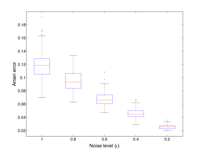
Figure 3: Performance of subspace averaging via Karcher mean.

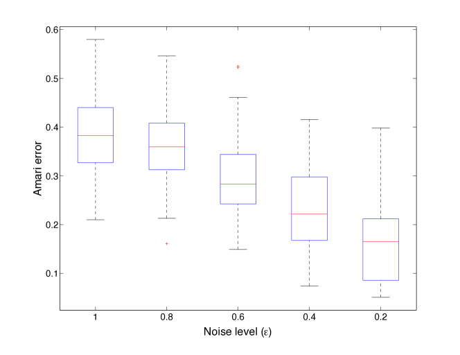
Figure 4: Performance of subspace averaging via Euclidean mean.

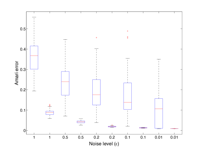
Figure 5: Comparison of performance (left = Euclidean, right = Karcher).

8 Conclusion

This work focuses on the problem of averaging complex subspaces of equal dimension by computing their Karcher mean, which is under mild assumptions the unique minimum of a well defined smooth function on the complex Grassmannian. An accessible introduction to the geometric structure of the Grassmanian is provided by its identification with the set of Hermitian projectors. In particular, explicit formulas for geodesics, parallel transport, and the Riemannian gradient of the Karcher mean function are given, which, in contrast to other formulas available in the literature, are well suited for implementation.

These results are used to propose an intrinsic conjugate gradient algorithm on the Grassmannian for computing the Karcher mean. We present experiments and outline the usability of such an approach in blind identification.

References

• Srivastava and Klassen [2004] A. Srivastava, E. Klassen, Bayesian and geometric subspace tracking, Advances in Applied Probability 36 (2004) 43–56.
• Adalı and Haykin [2010] T. Adalı, S. Haykin, Adaptive Signal Processing: Next Generation Solutions, Adaptive and Learning Systems for Signal Processing, Communications and Control, Wiley-IEEE Press, 2010.
• Turaga et al. [2011] P. Turaga, A. Veeraraghavan, A. Srivastava, R. Chellappa, Statistical computations on Grassmann and Stiefel manifolds for image and video-based recognition, IEEE Transactions on Pattern Analysis and Machine Intelligence 33 (2011) 2273–2286.
• Simonsson and Eldén [2010] L. Simonsson, L. Eldén, Grassmann algorithms for low rank approximation of matrices with missing values, BIT 50 (2010) 173–191.
• Karcher [1977] H. Karcher, Riemannian center of mass and mollifier smoothing, Commun. Pure Appl. Math. 30 (1977) 509–541.
• Kendall [1990] W. S. Kendall, Probability, convexity, and harmonic maps with small image. I: Uniqueness and fine existence, Proc. Lond. Math. Soc., III. Ser. 61 (1990) 371–406.
• Le [2001] H. Le, Locating Fréchet means with application to shape spaces, Adv. Appl. Probab. 33 (2001) 324–338.
• Gramkow [2001] C. Gramkow, On averaging rotations, J. Math. Im. Vis. 15 (2001) 7–16.
• Ando et al. [2004] T. Ando, C.-K. Li, R. Mathias, Geometric means, Linear Algebra Appl. 385 (2004) 305–334.
• Buss and Fillmore [2001] S. R. Buss, J. P. Fillmore, Spherical averages and applications to spherical splines and interpolation, ACM Trans. Graph. 20 (2001) 95–126.
• Kendall [1991] W. S. Kendall, Convexity and the hemisphere, J. Lond. Math. Soc., II. Ser. 43 (1991) 567–576.
• Corcuera and Kendall [1999] J. M. Corcuera, W. S. Kendall, Riemannian barycentres and geodesic convexity, Math. Proc. Camb. Philos. Soc. 127 (1999) 253–269.
• Absil et al. [2008] P.-A. Absil, R. Mahony, R. Sepulchre, Optimization algorithms on matrix manifolds, Princeton University Press, Princeton, NJ, 2008.
• Helmke et al. [2007] U. Helmke, K. Hüper, J. Trumpf, Newton’s method on Graßmann manifolds, 2007. ArXiv:0709.2205v2.
• Dreisigmeyer [2006] D. W. Dreisigmeyer, Direct Search Algorithms over Riemannian Manifolds, Technical Report, Los Alamos National Laboratory, USA, 2006.
• Absil et al. [2008] P.-A. Absil, R. Mahony, R. Sepulchre, Optimization Algorithms on Matrix Manifolds, Princeton University Press, Princeton, NJ, 2008.
• Kleinsteuber and Hüper [2007] M. Kleinsteuber, K. Hüper, An intrinsic CG algorithm for computing dominant subspaces, in: Proc. $32^{nd}$ IEEE Int. Conf. on Acoustics, Speech, and Signal Processing, Hawaii, USA, pp. IV1405–IV1408.
• Mittal and Meer [2012] S. Mittal, P. Meer, Conjugate gradient on Grassmann manifolds for robust subspace estimation, Image and Vision Computing (2012).
• Shen and Kleinsteuber [2010] H. Shen, M. Kleinsteuber, Complex blind source separation via simultaneous strong uncorrelating transform, in: Latent Variable Analysis and Signal Separation, volume 6365 of LNCS, Springer, 2010, pp. 287–294.
• do Carmo [1992] M. P. do Carmo, Riemannian geometry, Mathematics: Theory & Applications. Boston, MA: Birkhäuser, 1992.
• Kleinsteuber and Seghouane [2010] M. Kleinsteuber, A. Seghouane, A CG-type method for computing the dominant subspace of a symmetric matrix, 2010. Proc. of the 9th Portuguese Conf. on Automatic Control (CONTROLO’2010). CD-ROM.
• Nocedal and Wright [1999] J. Nocedal, S. J. Wright, Numerical optimization, Springer, 1999.
• Smith [1994] S. Smith, Optimization techniques on Riemannian manifolds, in: A. Bloch (Ed.), Hamiltonian and gradient flows, algorithms and control, AMS, Providence, 1994, pp. 113–136.
• Husemoller [1993] D. H. Husemoller, Fibre bundles. 3rd ed., Berlin: Springer-Verlag, 1993.
• Onishchik [1994] A. L. Onishchik, Topology of transitive transformation groups, Leipzig: Johann Ambrosius Barth, 1994.
• Hüper and Silva Leite [2007] K. Hüper, F. Silva Leite, On the geometry of rolling and interpolation curves on $S^{n}$, $\mathrm{SO}_{n}$, and Grassmann manifolds., J. Dyn. Control Syst. 13 (2007) 467–502.
• Sakai [1996] T. Sakai, Riemannian geometry, Translations of Mathematical Monographs. 149. Providence, RI: American Mathematical Society, 1996.
• Golub and Van Loan [1996] G. Golub, C. F. Van Loan, Matrix computations. 3rd ed., Baltimore, MD: The Johns Hopkins Univ. Press, 1996.
• Cichocki and Amari [2002] A. Cichocki, S.-I. Amari, Adaptive Blind Signal and Image Processing: Learning Algorithms and Applications, Wiley, 2002.
• Comon and Jutten [2010] P. Comon, C. Jutten (Eds.), Handbook of Blind Source Separation: Independent Component Analysis and Applications, Academic, 2010.
• Cardoso and Souloumiac [1993] J.-F. Cardoso, A. Souloumiac, Blind beamforming for non Gaussian signals, The IEE Proceedings of F 140 (1993) 363–370.
• Wax and Sheinvald [1997] M. Wax, J. Sheinvald, A least-squares approach to joint diagonalization, IEEE Signal Processing Letters 4 (1997) 52–53.
• Manton [2006] J. Manton, A centroid (Karcher mean) approach to the joint approximate diagonalisation problem: The real symmetric case, Digital Signal Processing 16 (2006) 468–478.
• Eriksson and Koivunen [2004] J. Eriksson, V. Koivunen, Complex-valued ICA using second order statistics, in: Proceedings of the $14^{th}$ IEEE International Workshop on Machine Learning for Signal Processing (MLSP 2004), pp. 183–191.
• Makino et al. [2007] S. Makino, T.-W. Lee, H. Sawada (Eds.), Blind Speech Separation, Signals and Communication Technology, Springer Netherlands, 2007.
• Amari et al. [1996] S. Amari, A. Cichocki, H. H. Yang, A new learning algorithm for blind signal separation, Advances in Neural Information Processing Systems 8 (1996) 757–763.